
Improving Seismic Fault Recognition with Self-Supervised Pre-Training: A Study of 3D Transformer-Based with Multi-Scale Decoding and Fusion


Abstract
1. Introduction
1.1. Background
1.2. Related Work
1.3. Motivation
2. Datasets
2.1. Datasets Employed
- Synthetic dataset
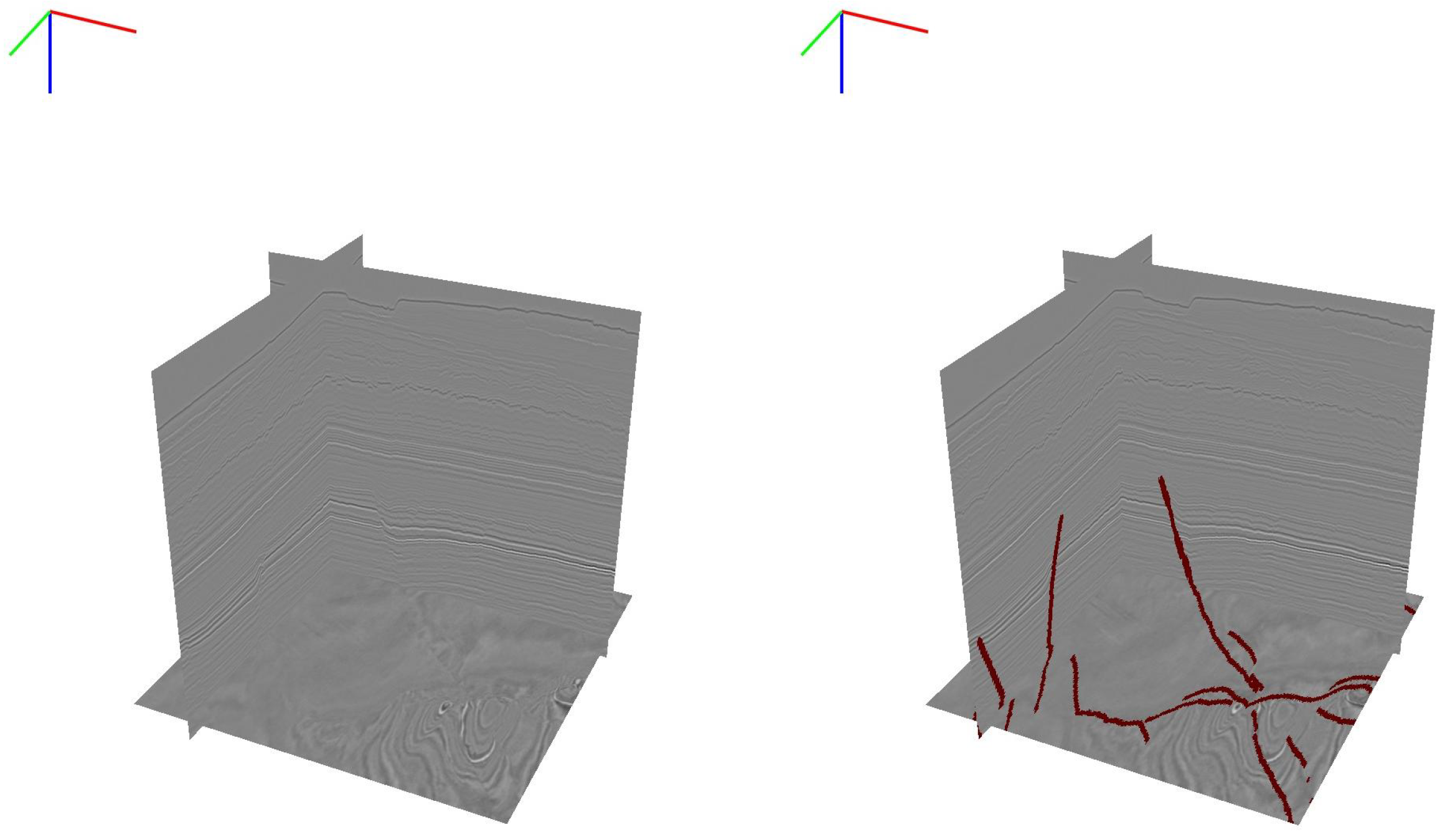
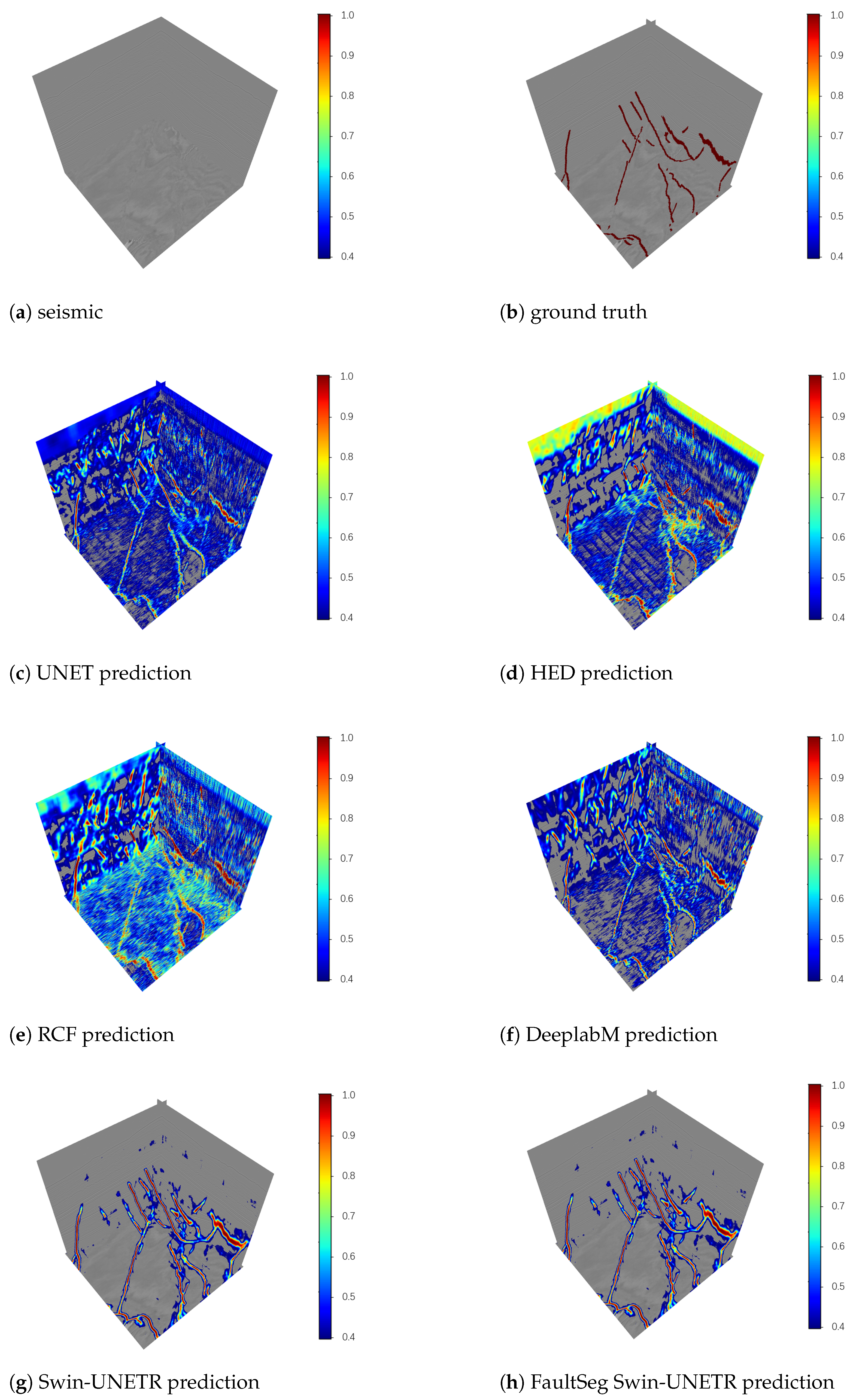
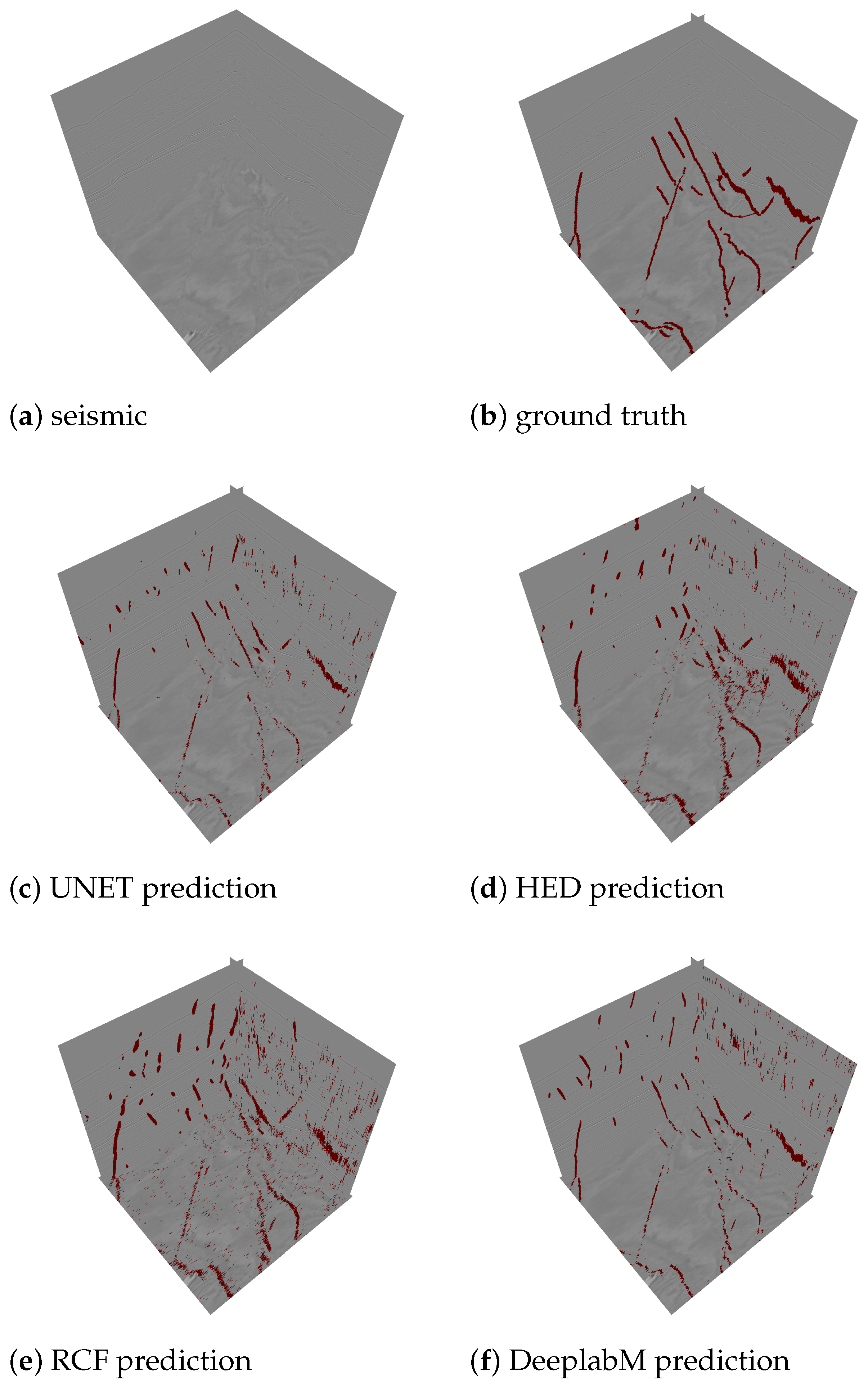
- Field datasetMost relevant works on fault recognition are trained on this synthetic dataset and then qualitatively analyzed on field fault datasets. However, deep learning methods typically require much training data to mitigate overfitting. Deep networks are prone to learning patterns specific to the synthetic data, which may not apply to real-world scenarios. Therefore, during the fine-tuning process, we conducted significant experiments using Thebe [40], the currently largest publicly available seismic faults dataset. The dataset, originally from a seismic survey called Thebe Gas Field in the Exmouth Plateau of the Carnarvan Basin on the NW shelf of Australia, is represented in Python Numpy format. The Thebe dataset has a size of . Because of the high correlation between adjacent slices, random partitioning along the crossline or inline direction was not a reasonable choice. Following the approach proposed by An et al. [40], we divided the data along the crossline direction. The first 900 slices were used for training, the next 200 for validation, and the remaining 703 for testing. The 640 × 640 × 640 cube segmented from the Thebe dataset is depicted in Figure 2. A comparison between Figure 1 and Figure 2 reveals that the field seismic data are comparatively more complex than the synthetic seismic data. The field seismic dataset exhibits a more intricate fault distribution and finer fault annotation lines, making transferring the model trained on synthetic data to field data challenging.
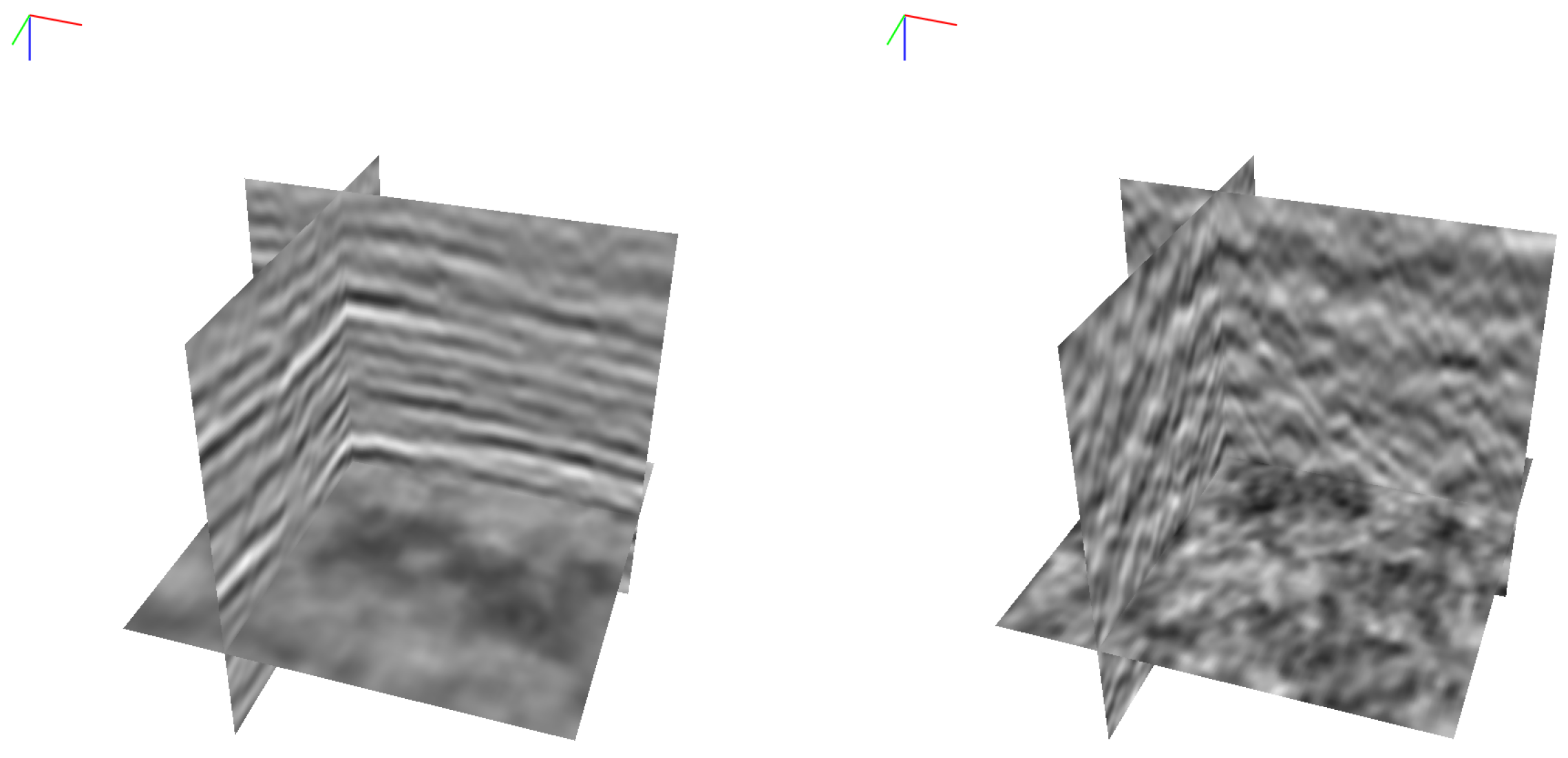
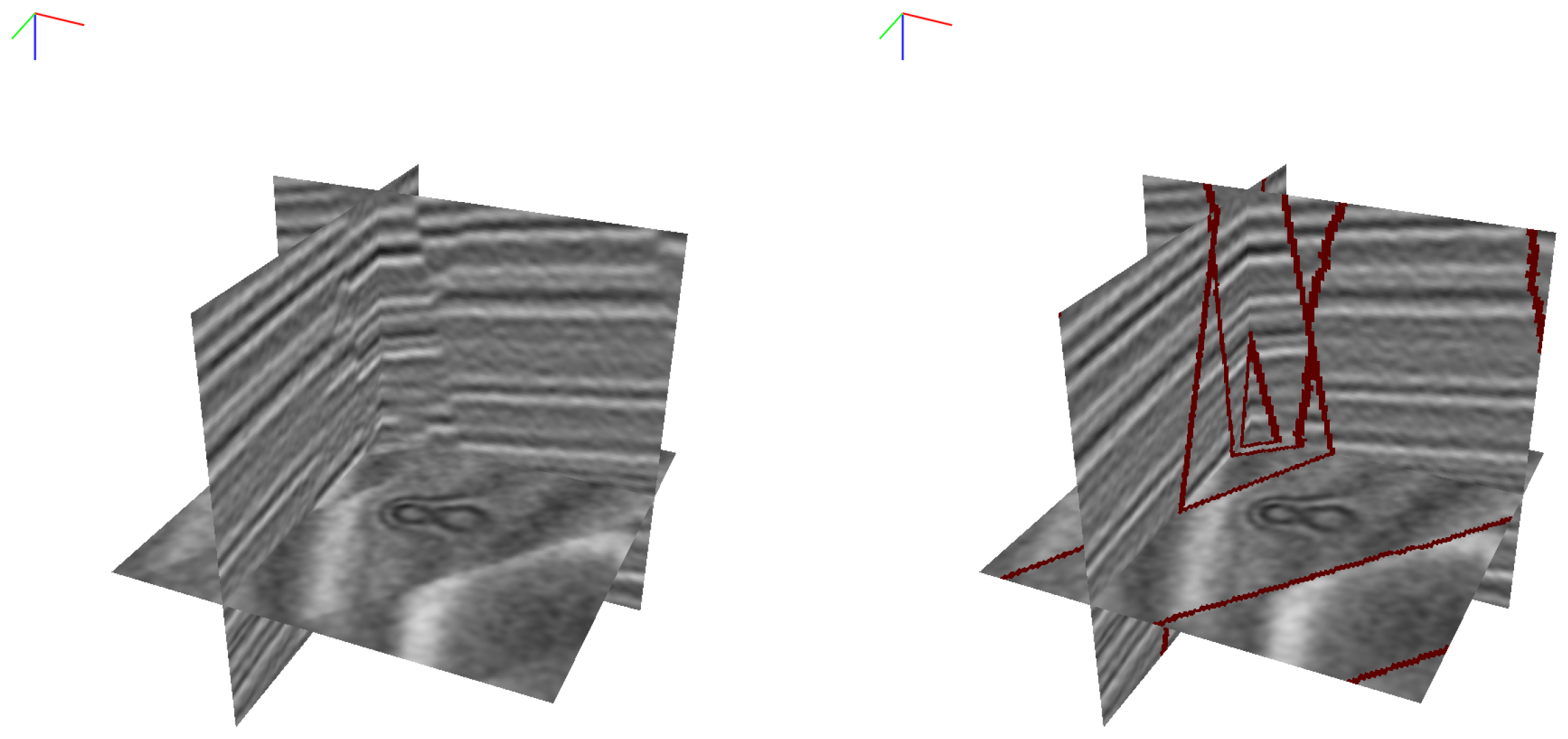
- Pre-training datasetIn addition, as self-supervised pre-training does not require annotations, we collected private datasets from 15 different working areas for pre-training tasks. These datasets are diverse in their geological features and size, and notably, they all lack fault annotations. Our goal was for the network to independently discover and learn the intrinsic characteristics of fault data across various contexts from various working areas during the self-supervised learning phase. We visualize some of the data used for pre-training in Figure 3.
2.2. Data Processing
3. Seismic Fault Recognition with Self-Supervised Pre-Training
3.1. Backbone and Pre-Training Methods
3.1.1. 3D Transformer-Based Backbone
3.1.2. Self-Supervised Pre-Training of Seismic Data
3.2. FaultSeg Swin-UNETR
3.2.1. Full-Network Pre-Training
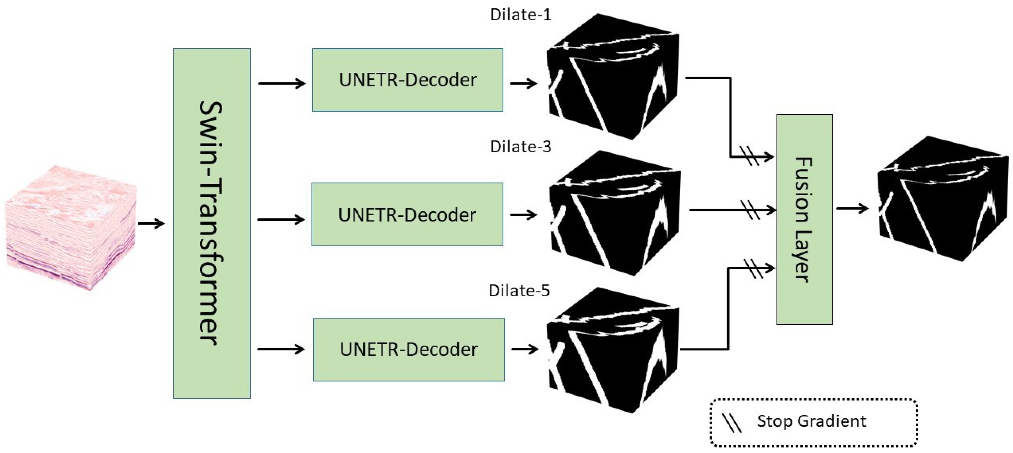
3.2.2. Multi-Scale Decoding and Fusion Module
4. Experimental Results and Analysis
4.1. Evaluation Metrics
4.2. Training and Validation
4.3. Results
4.4. Ablation Study
5. Discussion
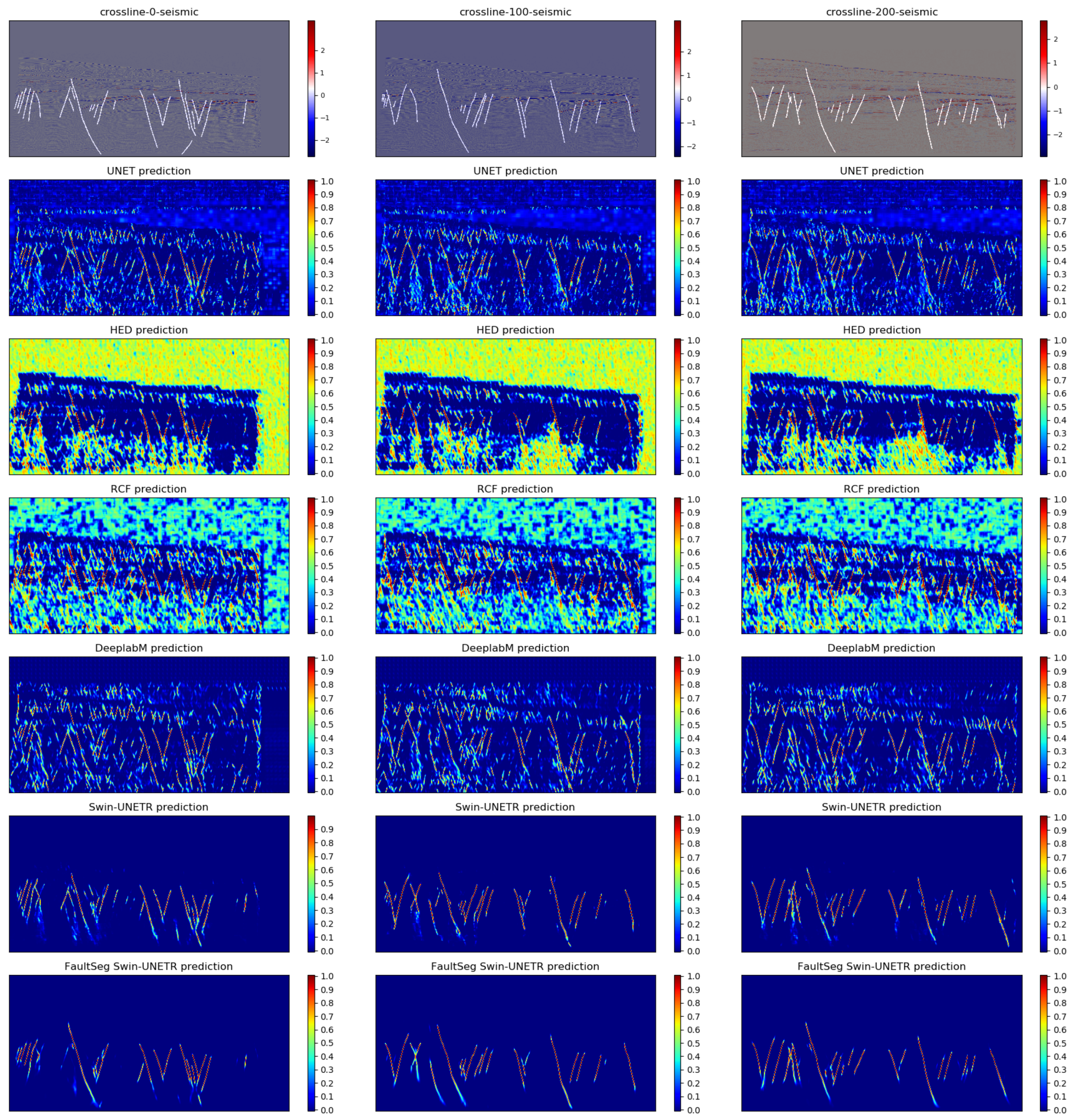
5.1. Performance of 2D Slices
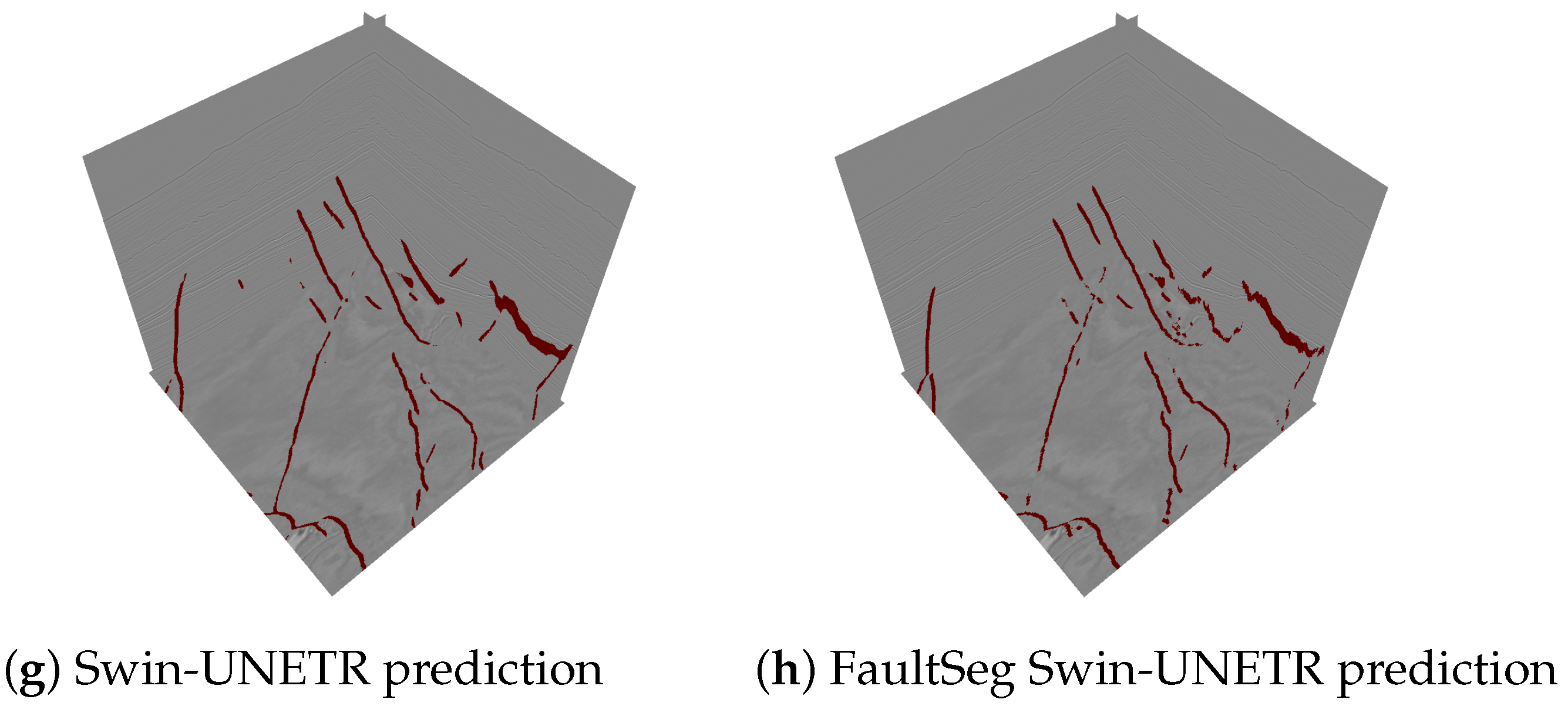
5.2. Performance of 3D Volumes
6. Conclusions
- Utilizing the 3D Swin-Transformer backbone network, we investigated diverse pre-training methods with a substantial volume of field 3D seismic data. The integration of SimMIM’s pre-training method with the enhanced Swin-UNETR model markedly improved performance. Consequently, we introduced FaultSeg Swin-UNETR, a method meticulously crafted for the unique characteristics of seismic data.
- We improved the Swin-UNETR model structure to adapt to the sparse distribution of seismic fault data and the narrow line profile characteristics in the inline or cross-line directions, promoting multi-scale decoding and fusion, thereby making fault detection easier.
- Furthermore, upon recognizing the significant imbalance in the number of parameters between the decoder and the backbone network in the Swin-UNETR model, we proposed a strategy for pre-training the complete segmentation model, which further improves fault detection accuracy.
- In the end, our proposed method achieves state-of-the-art performances on the Thebe dataset according to the standard metrics of the optimal image scale (OIS) and optimal dataset scale (ODS) metrics.
- Our research significantly advances the precision and efficiency of seismic fault recognition, overcoming the constraints associated with reliance on annotated datasets. This breakthrough paves the way for developing more robust and generalizable models capable of addressing the inherent complexities of field seismic data.
Author Contributions
Funding
Data Availability Statement
Acknowledgments
Conflicts of Interest
Appendix A

References
- Alcalde, J.; Bond, C.E.; Johnson, G.; Kloppenburg, A.; Ferrer, O.; Bell, R.; Ayarza, P. Fault interpretation in seismic reflection data: An experiment analysing the impact of conceptual model anchoring and vertical exaggeration. Solid Earth 2019, 10, 1651–1662. [Google Scholar] [CrossRef]
- Bouvier, J.; Kaars-Sijpesteijn, C.; Kluesner, D.; Onyejekwe, C.; Van der Pal, R. Three-dimensional seismic interpretation and fault sealing investigations, Nun River Field, Nigeria. AAPG Bull. 1989, 73, 1397–1414. [Google Scholar]
- Wu, X.; Geng, Z.; Shi, Y.; Pham, N.; Fomel, S.; Caumon, G. Building realistic structure models to train convolutional neural networks for seismic structural interpretation. Geophysics 2020, 85, WA27–WA39. [Google Scholar] [CrossRef]
- Fossen, H. Structural Geology; Cambridge University Press: New York, NY, USA, 2010; pp. 205–207. [Google Scholar]
- Posamentier, H.W.; Davies, R.J.; Cartwright, J.A.; Wood, L. Seismic Geomorphology—An Overview; Special Publications; Geological Society: London, UK, 2007. [Google Scholar]
- Knipe, R.J.; Jones, G.; Fisher, Q. Faulting, Fault Sealing and Fluid Flow in Hydrocarbon Reservoirs: An Introduction; Special Publications; Geological Society: London, UK, 1998. [Google Scholar]
- Ottesen Ellevset, S.; Knipe, R.; Svava Olsen, T.; Fisher, Q.; Jones, G. Fault Controlled Communication in the Sleipner Vest Field, Norwegian Continental Shelf: Detailed, Quantitative Input for Reservoir Simulation and Well Planning; Special Publications; Geological Society: London, UK, 1998; Volume 147, pp. 283–297. [Google Scholar]
- Richards, F.L.; Richardson, N.J.; Bond, C.E.; Cowgill, M. Interpretational Variability of Structural Traps: Implications for Exploration Risk and Volume Uncertainty; Geological Society: London, UK, 2015; Volume 421, pp. 7–27. [Google Scholar]
- Hale, D. Fault surfaces and fault throws from 3D seismic images. In Proceedings of the 2012 SEG Annual Meeting, Las Vegas, NV, USA, 4–9 November 2012. [Google Scholar]
- Stark, T.J. Unwrapping instantaneous phase to generate a relative geologic time volume. In Proceedings of the 2003 SEG Annual Meeting, Dallas, TX, USA, 26–31 October 2003. [Google Scholar]
- Wu, X.; Zhong, G. Generating a relative geologic time volume by 3D graph-cut phase unwrapping method with horizon and unconformity constraints. Geophysics 2012, 77, O21–O34. [Google Scholar] [CrossRef]
- Silva, C.C.; Marcolino, C.S.; Lima, F.D. Automatic fault extraction using ant tracking algorithm in the Marlim South Field, Campos Basin. In Proceedings of the 2005 SEG Annual Meeting, Houston, TX, USA, 6–11 November 2005. [Google Scholar]
- Pedersen, S.I.; Randen, T.; Sønneland, L.; Steen, Ø. Automatic fault extraction using artificial ants. In Proceedings of the 2002 SEG Annual Meeting, Salt Lake City, UT, USA, 6–9 October 2002. [Google Scholar]
- Figueiredo, A.M.; Gattass, M.; Szenberg, F. Seismic horizon mapping across faults with growing neural gas. In Proceedings of the 10th International Congress of the Brazilian Geophysical Society, Rio de Janeiro, Brazil, 19–23 November 2007. [Google Scholar]
- Zinck, G.; Donias, M.; Daniel, J.; Guillon, S.; Lavialle, O. Fast seismic horizon reconstruction based on local dip transformation. J. Appl. Geophys. 2013, 96, 11–18. [Google Scholar] [CrossRef]
- Wang, Z.; AlRegib, G. Automatic fault surface detection by using 3D Hough transform. In Proceedings of the 2014 SEG Annual Meeting, Denver, CO, USA, 26–31 October 2014. [Google Scholar]
- Bishop, C.M.; Nasrabadi, N.M. Pattern Recognition and Machine Learning; Springer: New York, NY, USA, 2006; Volume 4. [Google Scholar]
- Kortström, J.; Uski, M.; Tiira, T. Automatic classification of seismic events within a regional seismograph network. Comput. Geosci. 2016, 87, 22–30. [Google Scholar] [CrossRef]
- Guitton, A.; Wang, H.; Trainor-Guitton, W. Statistical imaging of faults in 3D seismic volumes using a machine learning approach. In SEG Technical Program Expanded Abstracts 2017; Society of Exploration Geophysicists: Houston, TX, USA, 2017; pp. 2045–2049. [Google Scholar]
- Zhao, T.; Mukhopadhyay, P. A fault detection workflow using deep learning and image processing. In Proceedings of the 2018 SEG International Exposition and Annual Meeting, Anaheim, CA, USA, 14–19 October 2018. [Google Scholar]
- Wu, X.; Shi, Y.; Fomel, S.; Liang, L. Convolutional neural networks for fault interpretation in seismic images. In Proceedings of the 2018 SEG International Exposition and Annual Meeting, Anaheim, CA, USA, 14–19 October 2018. [Google Scholar]
- Wu, X.; Liang, L.; Shi, Y.; Fomel, S. FaultSeg3D: Using synthetic data sets to train an end-to-end convolutional neural network for 3D seismic fault segmentation. Geophysics 2019, 84, IM35–IM45. [Google Scholar] [CrossRef]
- An, Y.; Guo, J.; Ye, Q.; Childs, C.; Walsh, J.; Dong, R. Deep convolutional neural network for automatic fault recognition from 3D seismic datasets. Comput. Geosci. 2021, 153, 104776. [Google Scholar] [CrossRef]
- Vaswani, A.; Shazeer, N.; Parmar, N.; Uszkoreit, J.; Jones, L.; Gomez, A.N.; Kaiser, Ł.; Polosukhin, I. Attention is all you need. In Proceedings of the 31st Conference on Neural Information Processing Systems (NIPS 2017), Long Beach, CA, USA, 4–9 December 2017; Volume 30. [Google Scholar]
- Dosovitskiy, A.; Beyer, L.; Kolesnikov, A.; Weissenborn, D.; Zhai, X.; Unterthiner, T.; Dehghani, M.; Minderer, M.; Heigold, G.; Gelly, S.; et al. An image is worth 16 × 16 words: Transformers for image recognition at scale. arXiv 2020, arXiv:2010.11929. [Google Scholar]
- Liu, Z.; Lin, Y.; Cao, Y.; Hu, H.; Wei, Y.; Zhang, Z.; Lin, S.; Guo, B. Swin transformer: Hierarchical vision transformer using shifted windows. In Proceedings of the IEEE/CVF International Conference on Computer Vision, Montreal, BC, Canada, 11–17 October 2021; pp. 10012–10022. [Google Scholar]
- He, K.; Chen, X.; Xie, S.; Li, Y.; Dollár, P.; Girshick, R. Masked autoencoders are scalable vision learners. In Proceedings of the IEEE/CVF Conference on Computer Vision and Pattern Recognition, New Orleans, LA, USA, 18–24 June 2022; pp. 16000–16009. [Google Scholar]
- Xie, Z.; Zhang, Z.; Cao, Y.; Lin, Y.; Bao, J.; Yao, Z.; Dai, Q.; Hu, H. Simmim: A simple framework for masked image modeling. In Proceedings of the IEEE/CVF Conference on Computer Vision and Pattern Recognition, New Orleans, LA, USA, 18–24 June 2022; pp. 9653–9663. [Google Scholar]
- Chen, T.; Kornblith, S.; Norouzi, M.; Hinton, G. A simple framework for contrastive learning of visual representations. PMLR 2020, 119, 1597–1607. [Google Scholar]
- Liu, B.; Jiang, P.; Wang, Q.; Ren, Y.; Yang, S.; Cohn, A.G. Physics-driven self-supervised learning system for seismic velocity inversion. Geophysics 2023, 88, R145–R161. [Google Scholar] [CrossRef]
- Monteiro, B.A.; Oliveira, H.; dos Santos, J.A. Self-Supervised Learning for Seismic Image Segmentation From Few-Labeled Samples. IEEE Geosci. Remote Sens. Lett. 2022, 19, 8028805. [Google Scholar] [CrossRef]
- Xu, Z.; Luo, Y.; Wu, B.; Meng, D.; Chen, Y. Deep Nonlocal Regularizer: A Self-Supervised Learning Method for 3D Seismic Denoising. IEEE Trans. Geosci. Remote. Sens. 2023, 61, 5921517. [Google Scholar] [CrossRef]
- Yang, J.; Wu, X.; Bi, Z.; Geng, Z. A multi-task learning method for relative geologic time, horizons, and faults with prior information and transformer. IEEE Trans. Geosci. Remote. Sens. 2023, 61, 5907720. [Google Scholar] [CrossRef]
- Tang, Z.; Wu, B.; Wu, W.; Ma, D. Fault Detection via 2.5 D Transformer U-Net with Seismic Data Pre-Processing. Remote Sens. 2023, 15, 1039. [Google Scholar] [CrossRef]
- Silva, R.M.; Baroni, L.; Ferreira, R.S.; Civitarese, D.; Szwarcman, D.; Brazil, E.V. Netherlands dataset: A new public dataset for machine learning in seismic interpretation. arXiv 2019, arXiv:1904.00770. [Google Scholar]
- Wang, Z.; You, J.; Liu, W.; Wang, X. Transformer assisted dual U-net for seismic fault detection. Front. Earth Sci. 2023, 11, 1047626. [Google Scholar] [CrossRef]
- Dou, Y.; Dong, M.; Li, K.; Xiao, Y. FaultSSL: Seismic Fault Detection via Semi-supervised learning. arXiv 2023, arXiv:2309.02930. [Google Scholar] [CrossRef]
- Tang, Y.; Yang, D.; Li, W.; Roth, H.R.; Landman, B.; Xu, D.; Nath, V.; Hatamizadeh, A. Self-supervised pre-training of swin transformers for 3d medical image analysis. In Proceedings of the IEEE/CVF Conference on Computer Vision and Pattern Recognition, New Orleans, LA, USA, 18–24 June 2022; pp. 20730–20740. [Google Scholar]
- An, Y.; Du, H.; Ma, S.; Niu, Y.; Liu, D.; Wang, J.; Du, Y.; Childs, C.; Walsh, J.; Dong, R. Current state and future directions for deep learning based automatic seismic fault interpretation: A systematic review. Earth-Sci. Rev. 2023, 243, 104509. [Google Scholar] [CrossRef]
- An, Y.; Guo, J.; Ye, Q.; Childs, C.; Walsh, J.; Dong, R. A gigabyte interpreted seismic dataset for automatic fault recognition. Data Brief 2021, 37, 107219. [Google Scholar] [CrossRef]
- Hatamizadeh, A.; Tang, Y.; Nath, V.; Yang, D.; Myronenko, A.; Landman, B.; Roth, H.R.; Xu, D. Unetr: Transformers for 3d medical image segmentation. In Proceedings of the IEEE/CVF Conference on Computer Vision and Pattern Recognition, New Orleans, LA, USA, 18–24 June 2022; pp. 574–584. [Google Scholar]
- An, Y.; Dong, R. Understanding the Effect of Different Prior Knowledge on CNN Fault Interpreter. IEEE Access 2023, 11, 15058–15068. [Google Scholar] [CrossRef]
- Dou, Y.; Li, K.; Zhu, J.; Li, T.; Tan, S.; Huang, Z. MD loss: Efficient training of 3-D seismic fault segmentation network under sparse labels by weakening anomaly annotation. IEEE Trans. Geosci. Remote Sens. 2022, 60, 5919014. [Google Scholar] [CrossRef]
- Kourehpaz, P.; Molina Hutt, C. Machine learning for enhanced regional seismic risk assessments. J. Struct. Eng. 2022, 148, 04022126. [Google Scholar] [CrossRef]
- Forcellini, D. An expeditious framework for assessing the seismic resilience (SR) of structural configurations. Structures 2023, 56, 105015. [Google Scholar] [CrossRef]
- Deng, J.; Dong, W.; Socher, R.; Li, L.J.; Li, K.; Fei-Fei, L. Imagenet: A large-scale hierarchical image database. In Proceedings of the 2009 IEEE Conference on Computer Vision and Pattern Recognition, Miami, FL, USA, 20–25 June 2009; pp. 248–255. [Google Scholar]
- Floridi, L.; Chiriatti, M. GPT-3: Its nature, scope, limits, and consequences. Minds Mach. 2020, 30, 681–694. [Google Scholar] [CrossRef]
- Kirillov, A.; Mintun, E.; Ravi, N.; Mao, H.; Rolland, C.; Gustafson, L.; Xiao, T.; Whitehead, S.; Berg, A.C.; Lo, W.Y.; et al. Segment anything. arXiv 2023, arXiv:2304.02643. [Google Scholar]


| Model Name | Backbone | Decode Head | Total Params |
|---|---|---|---|
| Swin-Transformer + Up Sample Net | 7.8 M | 3.1 M | 10.9 M |
| Swin-UNETR | 7.8 M | 54.1 M | 61.9 M |
| FaultSeg Swin-UNETR | 7.8 M | 93.3 M | 101.1 M |
| Model | Pre-Trained Method | OIS | ODS |
|---|---|---|---|
| UNet | - | 0.769 | 0.766 |
| HED | - | 0.811 | 0.806 |
| RCF | - | 0.806 | 0.800 |
| DeeplabM | - | 0.759 | 0.756 |
| DeeplabV3 | Imagenet-pre-trained | 0.849 | 0.845 |
| FaultSeg3D | - | 0.840 | 0.836 |
| UNETR | - | 0.845 | 0.841 |
| UNETR | SimCLR | 0.849 | 0.845 |
| UNETR | MAE | 0.847 | 0.844 |
| UNETR | SimMIM | 0.846 | 0.843 |
| Swin-UNETR | - | 0.844 | 0.840 |
| Swin-UNETR | Three-task-pre-trained | 0.852 | 0.845 |
| Swin-UNETR | SimCLR | 0.855 | 0.852 |
| Swin-UNETR | MAE | 0.859 | 0.857 |
| Swin-UNETR | SimMIM | 0.861 | 0.857 |
| Swin-UNETR | Overall SimMIM | 0.872 | 0.868 |
| FaultSeg Swin-UNETR | - | 0.851 | 0.847 |
| FaultSeg Swin-UNETR | SimMIM | 0.866 | 0.862 |
| FaultSeg Swin-UNETR | Overall SimMIM | 0.875 | 0.870 |
| Model | Pre-Trained Method | OIS | ODS |
|---|---|---|---|
| FaultSeg3D | - | 0.441 | 0.431 |
| Swin-UNETR | Three-task-pre-trained | 0.482 | 0.473 |
| Swin-UNETR | SimMIM | 0.503 | 0.495 |
| FaultSeg Swin-UNETR | Overall SimMIM | 0.525 | 0.510 |
| Model | Chunk Size | OIS | ODS |
|---|---|---|---|
| Swin-UNETR | 0.830 | 0.827 | |
| 0.841 | 0.835 | ||
| 0.844 | 0.840 | ||
| 0.832 | 0.829 |
| Model | Positive Weight | OIS | ODS |
|---|---|---|---|
| Swin-UNETR | 1.0 | 0.844 | 0.840 |
| 5.0 | 0.845 | 0.839 | |
| 10.0 | 0.843 | 0.841 |
Disclaimer/Publisher’s Note: The statements, opinions and data contained in all publications are solely those of the individual author(s) and contributor(s) and not of MDPI and/or the editor(s). MDPI and/or the editor(s) disclaim responsibility for any injury to people or property resulting from any ideas, methods, instructions or products referred to in the content. |
© 2024 by the authors. Licensee MDPI, Basel, Switzerland. This article is an open access article distributed under the terms and conditions of the Creative Commons Attribution (CC BY) license (https://creativecommons.org/licenses/by/4.0/).
Share and Cite
Zhang, Z.; Chen, R.; Ma, J. Improving Seismic Fault Recognition with Self-Supervised Pre-Training: A Study of 3D Transformer-Based with Multi-Scale Decoding and Fusion. Remote Sens. 2024, 16, 922. https://doi.org/10.3390/rs16050922
Zhang Z, Chen R, Ma J. Improving Seismic Fault Recognition with Self-Supervised Pre-Training: A Study of 3D Transformer-Based with Multi-Scale Decoding and Fusion. Remote Sensing. 2024; 16(5):922. https://doi.org/10.3390/rs16050922
Chicago/Turabian StyleZhang, Zeren, Ran Chen, and Jinwen Ma. 2024. "Improving Seismic Fault Recognition with Self-Supervised Pre-Training: A Study of 3D Transformer-Based with Multi-Scale Decoding and Fusion" Remote Sensing 16, no. 5: 922. https://doi.org/10.3390/rs16050922
APA StyleZhang, Z., Chen, R., & Ma, J. (2024). Improving Seismic Fault Recognition with Self-Supervised Pre-Training: A Study of 3D Transformer-Based with Multi-Scale Decoding and Fusion. Remote Sensing, 16(5), 922. https://doi.org/10.3390/rs16050922