Article

Multi-Level Feature-Refinement Anchor-Free Framework with Consistent Label-Assignment Mechanism for Ship Detection in SAR Imagery

School of Information Communication and Engineering, University of Electronic Science and Technology of China, Chengdu 611731, China
*
Author to whom correspondence should be addressed.
Remote Sens. 2024, 16(6), 975; https://doi.org/10.3390/rs16060975
Submission received: 13 January 2024 / Revised: 6 March 2024 / Accepted: 7 March 2024 / Published: 10 March 2024

Abstract

:
Deep learning-based ship-detection methods have recently achieved impressive results in the synthetic aperture radar (SAR) community. However, numerous challenging issues affecting ship detection, such as multi-scale characteristics of the ship, clutter interference, and densely arranged ships in complex inshore, have not been well solved so far. Therefore, this article puts forward a novel SAR ship-detection method called multi-level feature-refinement anchor-free framework with a consistent label-assignment mechanism, which is capable of boosting ship-detection performance in complex scenes. First, considering that SAR ship detection is susceptible to complex background interference, we develop a stepwise feature-refinement backbone network to refine the position and contour of the ship object. Next, we devise an adjacent feature-refined pyramid network following the backbone network. The adjacent feature-refined pyramid network consists of the sub-pixel sampling-based adjacent feature-fusion sub-module and adjacent feature-localization enhancement sub-module, which can improve the detection capability of multi-scale objects by mitigating multi-scale high-level semantic loss and enhancing low-level localization features. Finally, to solve the problems of unbalanced positive and negative samples and densely arranged ship detection, we propose a consistent label-assignment mechanism based on consistent feature scale constraints to assign more appropriate and consistent labels to samples. Extensive qualitative and quantitative experiments on three public datasets, i.e., SAR Ship-Detection Dataset (SSDD), High-Resolution SAR Image Dataset (HRSID), and SAR-Ship-Dataset illustrate that the proposed method is superior to many state-of-the-art SAR ship-detection methods.

1. Introduction

Thanks to its unique operating characteristics, including all-weather, all-day and all-night, and long-distance, synthetic aperture radar (SAR) has a broad range of application prospects in military and civil fields, such as maritime domain awareness, energy exploration, battle situation awareness, and so forth. Ship object detection is the primary stage of SAR image interpretation in maritime domain awareness, which is bound to affect the reliability of subsequent object recognition. Nevertheless, due to the uncertainty of sea clutter, the diversity of ship scales, and the interference from land clutter, ship detection appears to be one of the most challenging tasks in the field of SAR image interpretation.
In the early years, constant false alarm rate (CFAR), as a kind of classic detection model, has been extensively investigated in SAR ship detection. Under the premise of a CFAR, a CFAR detector can adaptively adjust the detection threshold according to the statistical distribution of clutter, therefore distinguishing ship objects from complex backgrounds [1]. In view of the excellent performance of CFAR detector in SAR ship detection, various extensions of CFAR have been proposed in succession [2,3,4]. For instance, Qin et al. [5] exploited the generalized gamma distribution to model the background clutter and achieved more satisfactory performance than other parametric distribution-based CFAR detectors. Pappas et al. [6] presented a CFAR detector based on superpixel level, which aims to reduce the probability of false alarms through superpixel technology. Gao et al. [7] proposed a statistical model based on the gamma distribution to achieve ship object detection in a non-homogeneous sea-clutter background. The reliability of the detection results of CFAR is closely related to the detection threshold determined by the statistical distribution of clutter. However, it is extremely challenging to artificially analyze the characteristics of clutter and ships in complex backgrounds, especially offshore with severe interference and noise. In addition, the CFAR-based ship-detection method cannot be learned in an end-to-end way due to the cumbersome parameter settings, resulting in a tedious detection process and low efficiency.
With the flourishing development of deep learning technology, deep learning-based object detection has recently achieved significant advancement. In a broad sense, deep learning-based detection methods can be grouped into two categories, i.e., two-stage method and one-stage method. Among them, various models of the Region-based Convolutional Neural Network (R-CNN) series [8,9,10] are typical representatives of the two-stage method, which integrates the top-down region proposal with the rich features of convolutional neural network computation to greatly improve the detection effect of ship objects. The two-stage method can obtain desirable detection accuracy through region proposals, but the shortcoming of this kind of algorithm is low real-time. To improve the real-time performance of detection, a new two-stage detection model named Faster R-CNN [11] is developed, which cleverly integrates feature extraction, region proposal, bounding box regression, and classification into a unified network. To solve three imbalance problems, including sample level, feature level, and objective level, Pand et al. proposed a new detection method called Libra R-CNN [12], which can achieve better detection performance without major changes in the network structure. By contrast, one-stage method, such as RetinaNet [13], YOLO [14,15,16], and SSD [17,18], is dedicated to boosting the detection efficiency at the expense of certain accuracy. Currently, the detection methods of the YOLO family have become the mainstream of the one-stage detection method.
In the beginning, regardless of two-stage models or one-stage models, a large body of anchor boxes should be preset in the process of object detection. Anchor-based methods, such as Faster R-CNN, RetinaNet, and YOLO, can achieve proud detection accuracy with the help of predefined anchor boxes but encounter trouble in the face of multi-scale ship-detection tasks. The emergence of anchor-free methods such as fully convolutional one-Stage (FCOS) [19] object detection based on pixel level prediction, you only look once (YOLOX) [20], etc., not only overcomes the defects of anchor-based methods but also simplifies the detection procedure in a sense. Later, Zhang et al. proposed an adaptive training sample selection (ATSS) [21] to investigate the gap between anchor-based and anchor-free detection. Zhu et al. proposed a feature selective anchor-free (FSAF) [22] module to address the challenge of multi-scale objects.
Up to now, large quantities of deep learning-based detection methods have emerged and achieved wonderful performance in the field of natural images. Nevertheless, due to the diversity of ship scales and strong clutter interference in large-scale SAR scenarios, it is infeasible to directly transfer existing detection models from computer vision to SAR ship detection. To overcome these challenging problems, scholars have put much effort into deep learning-based ship detection and proposed many ship-detection algorithms with impressive results [23,24,25,26,27]. For instance, Cui et al. developed a new detection framework named dense attention pyramid network to achieve multi-scale dense SAR ship detection [28]. Based on CenterNet [29], Guo et al. developed a one-stage detector called CenterNet++ to solve the problem of small-scale SAR ship detection [30]. Under the framework of FCOS, Sun et al. proposed an anchor-free SAR ship detection method, which redefined the positive and negative sample label-assignment method to reduce interference from background clutter and overlapping bounding boxes [31]. Inspired by the benefits of the YOLOX framework, Wan et al. developed an anchor-free detection method called AFSar to achieve ship detection in complex SAR scenes [32]. Hu et al. proposed a balanced attention network (BANet) integrating local attention and global attention to promote the performance of multi-scale SAR ship detection [33].
Although deep learning-based ship-detection methods have shown considerably superior detection results than the traditional detectors, there are still the following challenges that scholars are still trying to explore and solve [34,35]. First, there is strong noise and serious clutter interference in the process of ship feature extraction due to the mechanism of SAR coherent imaging. Second, the diversity of ship scales, especially small-scale ships in large-scale scenes, greatly increases the difficulty of detection. Finally, it is prone to miss detection and false alarms inshore because of complex land clutter and densely arranged ships.
In response to these intractable obstacles mentioned above, based on the anchor-free detection framework, we propose a one-stage anchor-free detector named multi-level feature-refinement anchor-free framework with a consistent label-assignment mechanism in this article. The main contributions of this article are summarized as follows:
  • A one-stage anchor-free detector named multi-level feature-refinement anchor-free framework with a consistent label-assignment mechanism is proposed to boost the detection performance of SAR ships in complex scenes. A series of qualitative and quantitative experiments on three public datasets, SSDD, HRSID, and SAR-Ship-Dataset, demonstrate that the proposed method outperforms many state-of-the-art detection methods.
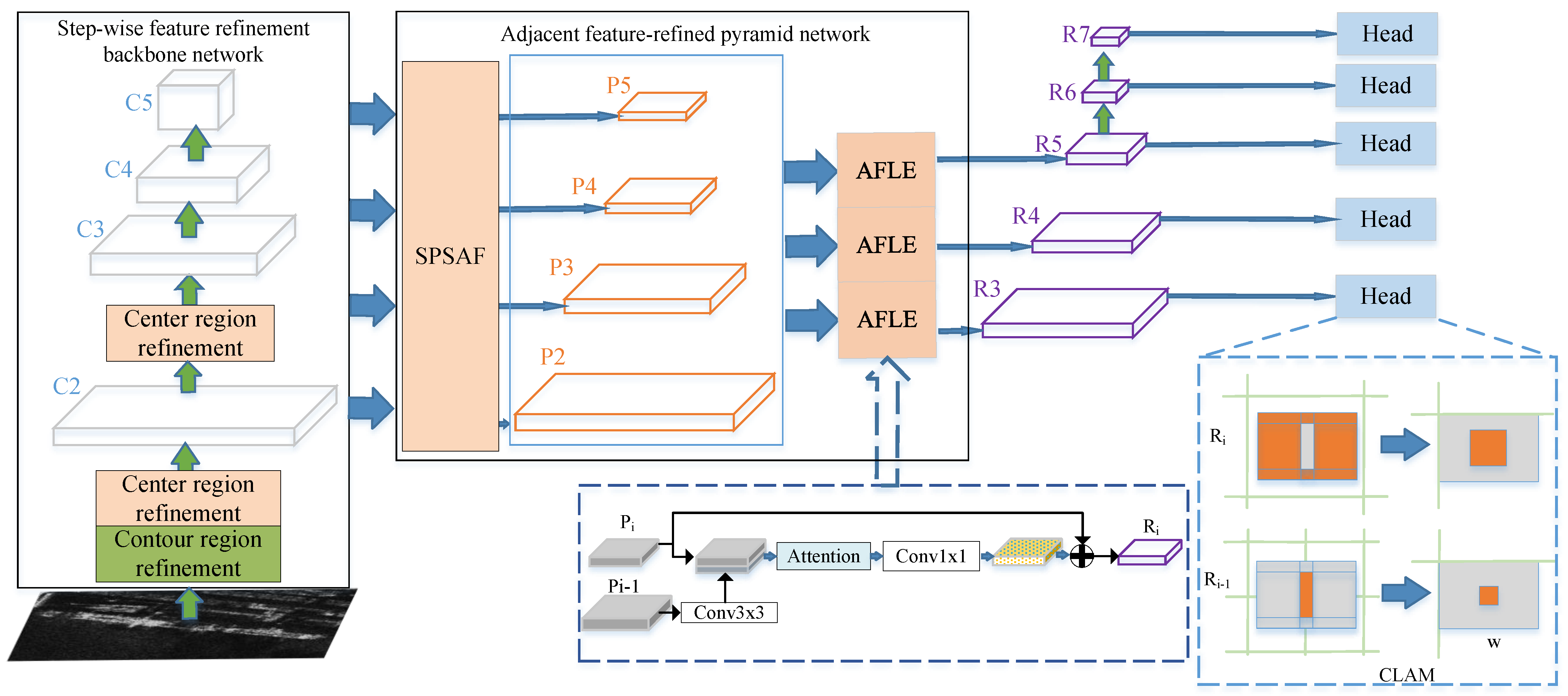
  • To extract abundant ship features while suppressing complex background clutter, a stepwise feature-refinement backbone network is proposed, which refines the position and contour of the ship in turn via stepwise spatial information decoupling function, therefore improving ship-detection performance.
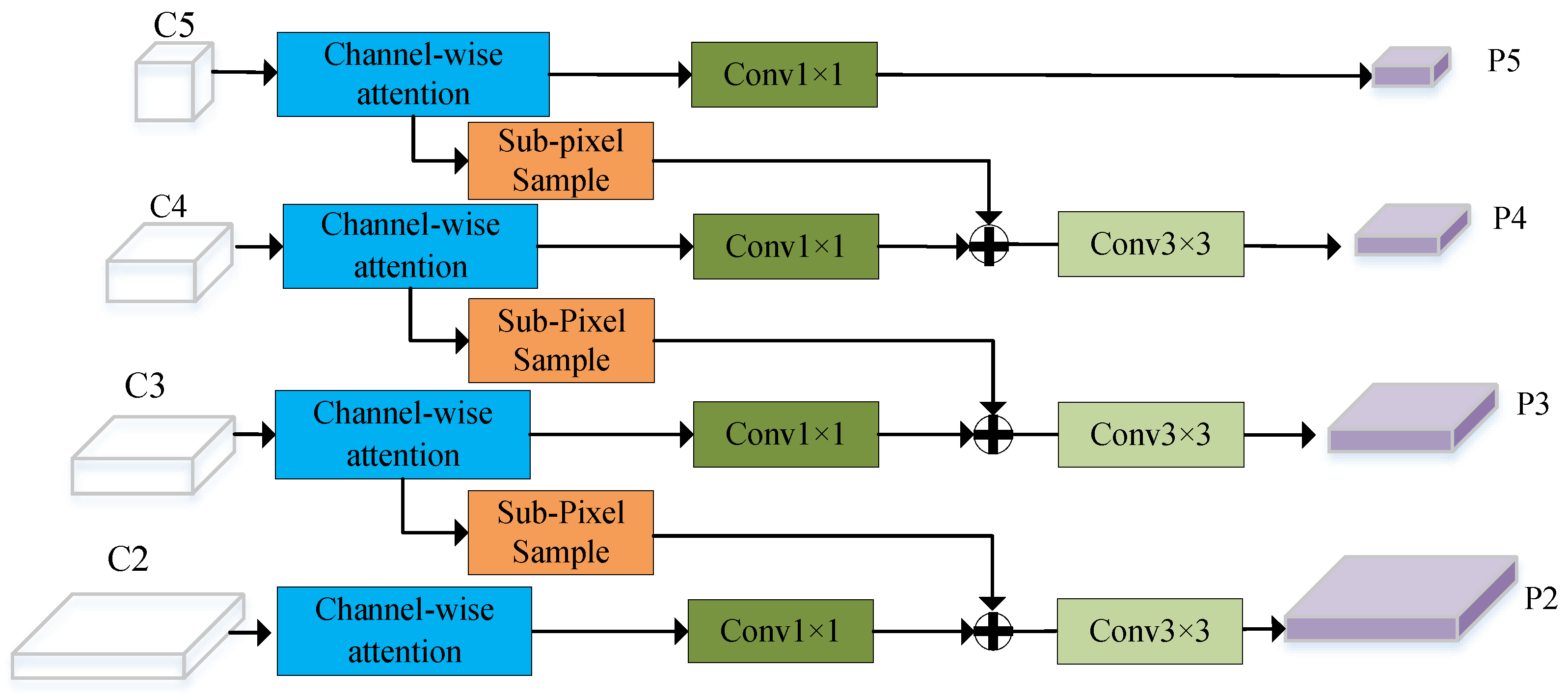
  • To effectively fuse the multi-scale features of the ships and avoid the semantic aliasing effect in cross-scale layers, an adjacent feature-refined pyramid network consisting of sub-pixel sampling-based adjacent feature-fusion sub-module and adjacent feature-localization enhancement sub-module is proposed, which is beneficial for multi-scale ship detection by alleviating multi-scale high-level semantic loss and enhancing low-level localization features at the adjacent feature layers.
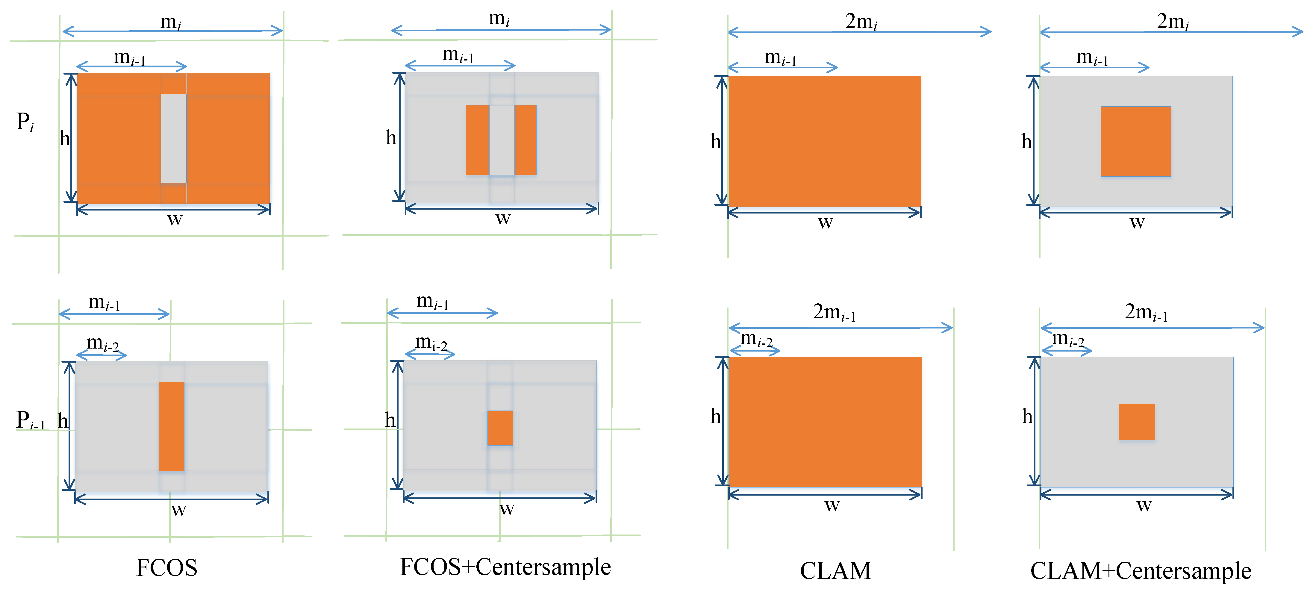
  • In light of the problem of unbalanced label assignment of samples in one-stage anchor-free detection, a consistent label-assignment mechanism based on consistent feature scale constraints is presented, which is also beneficial in meeting the challenges of dense prediction, especially densely arranged ships inshore.
The remainder of this article is organized as follows. Section 2 elaborates on key components of the proposed multi-level feature-refinement anchor-free framework with a consistent label-assignment mechanism. In Section 3, we conduct extensive experiments on SSDD, HRSID, and SAR-Ship-Dataset to demonstrate the effectiveness of the proposed method. Section 4 concludes this article.

2. Methodology

In this article, the proposed method is composed of three key components: (i) stepwise feature-refinement backbone network, (ii) adjacent feature-refined pyramid network, and (iii) consistent label-assignment mechanism, as depicted in Figure 1. In the following, the theory and network architecture of each component are elaborated.

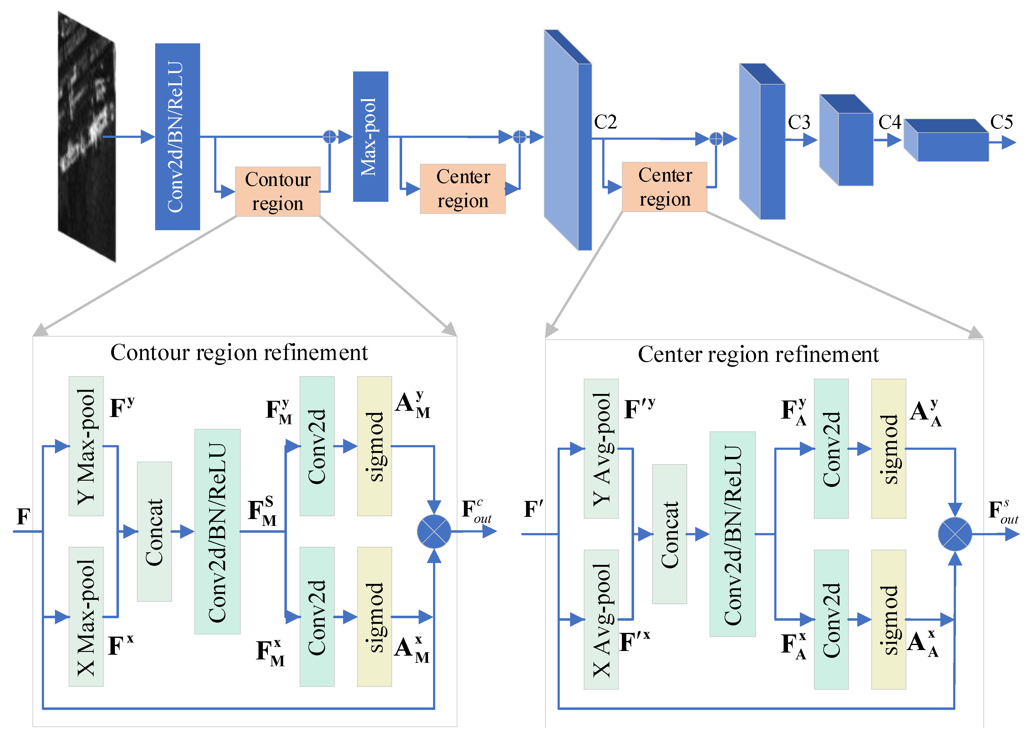
2.1. Stepwise Feature-Refinement Backbone Network

Under the framework of deep learning-based ship detection, the backbone network is the essential component to extract the deep semantic features of the ship from large-scale SAR scenes. In contrast to optical imagery and infrared imagery, the feature extraction of SAR ship objects is particularly susceptible to background clutter and noise due to the unique SAR imaging mechanism. Inspired by the existing work [36,37,38], this article proposes a novel feature extraction method named stepwise feature-refinement (SwFR) backbone network. Concretely speaking, we introduce the idea of stepwise feature refinement into the backbone network to facilitate ship position regression and foreground and background classification in complex SAR scenes. It is worth emphasizing that the difference between the proposed stepwise feature-refinement method and the existing work [36] is that the proposed method not only considers the central region refinement to facilitate object position regression but also refines the contour region to facilitate object detection. Let F R C × H × W be the feature map of the ship object, where C denotes the number of feature channels, W and H represent the sizes of the feature map in the horizontal and vertical directions, respectively.
To highlight the contour of the ship object, we first decouple the spatial information into the horizontal direction and the vertical direction through a one-dimensional max-pooling operation. The features in different directions after decoupling can be expressed as:
F x = m a x y H F ( x , y )
F y = m a x x W F ( x , y )
where m a x ( · ) represents the maximum response operation, F ( x , y ) is the input two-dimensional feature map, F x and F y are one-dimensional feature maps along two directions. The above two operations can capture long-range dependencies along one spatial direction while acquiring location information along other direction, which is conductive to helping the model more accurately locate the object of interest.
Then, to encode spatial information in both the horizontal direction and the vertical direction, we concatenate the features obtained in Equations (1) and (2) and send them into a convolutional layer with the kernel size of 1 × 1, yielding:
F M s = σ C o n v C o n c a t F x , F y
where F M s R C / r × H × W , C o n c a t ( · ) represents the concatenation operation, C o n v denotes the convolution operation, σ is a nonlinear activation function, and r is a compression ratio.
Afterward, F M s is split to obtain F M x R C / r × W and F M y R C / r × H along two different spatial dimensions. In order to ensure that the number of channels of F M x R C / r × W and F M y R C / r × H , is consistent with that of F , two 1 × 1 convolution operations are exploited to transform F M x and F M y . The attention maps along different directions are then obtained according to the following operation:
A M x = δ C o n v F M x
A M y = δ C o n v F M y
where δ is the sigmoid activation function. The outputs A M x and A M y are utilized as attention weights, respectively.
The above operations based on max-pooling can effectively locate the contour region of the target along different spatial directions. Finally, the features after highlighting the contour of the ship object can be expressed as:
F o u t c = F × A M x × A M y
To highlight the center region of the ship object for effectively performing position regression, we first decouple the spatial information into the horizontal direction and the vertical direction through a one-dimensional average pooling operation. The features in different directions after decoupling can be represented as follows:
F x = 1 H y H F x , y
F y = 1 W x W F x , y
where F x , y is the input two-dimensional feature map, F x and F y are one-dimensional feature maps.
Then, similar to ship contour refinement operations, the attention maps that can highlight the ship center region along different directions can be obtained according to the following formula:
A A x = δ C o n v F A x
A A y = δ C o n v F A y
Finally, the features after highlighting the center of the ship object can be expressed as:
F o u t s = F × A A x × A A y
The network architecture of contour region refinement and center region refinement are shown in Figure 2. Considering that information such as contour and position are low-level features of ship objects, we sequentially deploy the contour refinement function and central region refinement function in the shallow layer of the backbone network. In addition, we argue that the ship region is more prominent after contour refinement. Based on the above analysis, the architecture of the SwFR backbone network is depicted in Figure 2. The modules in the original ResNet backbone are shown in blue. C 2 , C 3 , C 4 , C 5 are the feature maps extracted from the proposed backbone network at different levels.

2.2. Adjacent Feature-Refined Pyramid Network

Feature pyramid network (FPN) [39] is responsible for aggregating information across levels so that the features at each level have abundant semantic information, which is very conducive to multi-scale object detection tasks. However, existing ship detectors with FPN suffer from two inherent shortcomings. On the one hand, the channel reduction at the high-level information layers brings about the loss of semantic information. On the other hand, miscellaneous cross-scale feature fusion may give rise to serious aliasing effects. For this purpose, we propose an extended version of FPN named adjacent feature-refined pyramid network (AFRPN), which consists of a top-down sup-pixel sampling-based adjacent feature-fusion (SPSAF) sub-module and a bottom-up adjacent feature-localization enhancement (AFLE) sub-module. The proposed AFRPN is located at the neck of the detection network, i.e., in the second component, as shown in Figure 1. During training, the two submodules are learned simultaneously to effectively utilize high-level semantic information and low-level localization information.
In the top-down SPSAF sub-module, channel-wise attention is first deployed along channels of different scales to adaptively select and highlight important channel features. Afterward, we introduce sup-pixel convolution [40] instead of the traditional convolution with the kernel size of 1 × 1 to execute channel transform and upsampling, which is intended to mitigate channel information loss. Then, the convolutional operation with the kernel size of 1 × 1 is exploited to adjust the dimension of channels to facilitate cross-layer fusion of multi-scale features.
It is worth emphasizing that the fusion operation at different scales is only performed on adjacent feature layers to mitigate the aliasing effects caused by miscellaneous feature cross-layer fusion. To effectively integrate the semantic information between adjacent feature layers, the convolutional operation with the kernel size of 3 × 3 is used, which is also conducive to reducing the aliasing effects caused by the pixel-wise addition on the feature maps. The overall architecture of the SPSAF sub-module is depicted in Figure 3.
C 2 , C 3 , C 4 , C 5 are the input feature maps of the SPSAF module. To refine the features along the channel level, we exploit a channel-wise weighting function defined in SENet [41]. Meanwhile, a convolution operation with a kernel size of 1 × 1 is used to adjust the number of the features, i.e.,
C i = F c w a ( C i ) , i = 2 , 3 , 4 , 5
I i = Φ C i , i = 2 , 3 , 4 , 5
where F c w a represents a channel-wise weighting function, Φ denotes the convolution operation with the kernel size of 1 × 1 .
The sub-pixel upsampling can convert low-resolution feature maps to high-resolution feature maps by pixel rearrangement in a specific order [42]. Mathematically, the sub-pixel upsampling operation can be defined as
PS ( C ) x , y , c = C x / r , y / r , M · r · mod ( y , r ) + M · m o d ( x , r ) + c
where r denotes the upsampling factor, m o d ( · , · ) represents the operation of taking the remainder, and PS ( C ) x , y , c denotes the output pixel on coordinates ( x , y , c ) . Considering that the upsampling operation is performed between adjacent feature layers, r is set to 2 in this article. The output of the SPSAF sub-module is described as
P i = I i , Ψ ( I i + Φ ( PS ( C i + 1 ) ) ) , Ψ ( I i + PS ( C i + 1 ) ) , Ψ ( I i + PS ( Φ ( C i + 1 ) ) ) , i = 5 i = 4 i = 3 i = 2
where Ψ represents the convolutional operation with the kernel size of 3 × 3 .
To make full use of low-level information for accurately locating ship objects, an adjacency feature-localization enhancement (AFLE) sub-module is developed, whose network architecture is illustrated in Figure 1. In the AFLE sub-module, the lower-level feature map P i 1 is first converted to the same size as the higher-level feature map P i by the convolutional operation with the kernel size of 3 × 3 , and then the features between adjacent layers are fused by concatenation operation along channel dimension, yielding:
F i = Concat P i , Ψ P i 1 , i = 3 , 4 , 5
Afterward, we introduce the idea of attention [37] to highlight localization information at both channel and spatial levels, i.e.,
F i = M C F i F i
F i = M S F F i
where M C is a one-dimension channel attention map, and M S is a two-dimension spatial attention map, their calculation process can be referenced in the literature [37]. Drawing lessons from the merits of residual learning, the AFLE module reduces the channel of the weighted feature map F i to 256 dimensions through a convolution with the kernel size of 1 × 1 , and then adds it to the residual block P i . By so doing, an enhanced output feature map R i can be obtained. The overall output feature maps can be expressed as:
R i = P i + Φ F i , Ψ R i 1 , i = 3 , 4 , 5 i = 6 , 7
We leverage three AFLE modules to obtain outputs R 3 , R 4 , R 5 , R 6 , R 7 are obtained by the convolutional downsampling operations on R 5 .

2.3. Consistent Label-Assignment Mechanism

The definition and assignment method of sample labels can directly affect the training efficiency and detection accuracy of the model. However, current anchor-free ship-detection methods suffer from two deficiencies in terms of sample label assignment. One is that, in some situations, the label definitions of positive and negative samples are semantically confusing. Another is that the existing anchor-free ship-detection methods assign the sample points in the overlapping area to the ground-truth (GT) box with the smallest region, which is not suitable for detecting dense SAR ships with very close scales. To this end, this article proposes a consistent label-assignment mechanism (CLAM) based on consistent feature scale constraints to assign more appropriate and consistent labels to samples, therefore promoting the detection performance of the model.
For each location ( x , y ) on the feature map R i , its location mapped to the original SAR image can be calculated according to the following formula:
x 1 , y 1 = s 2 + x s , s 2 + y s
where s is the stride of the feature map R i .
The location ( x , y ) is labeled as a negative sample if the corresponding point ( x 1 , y 1 ) fails to fall inside any GT boxes. For those sample points that fall inside the GT box, constraints should be set on the regression distance of these points. Herein, a 4-dimensional vector l * , r * , t * , b * is defined, which is exploited to calculate the distance between the point to the four sides of the GT box as the regression objective. Formally, if the location (x, y) is associated with any GT box, where the GT box is described as B = x m i n , y m i n , x m a x , y m a x by the coordinates of left-top and right-bottom corners, the regression objective for this location can be expressed as:
l * = x 1 x m i n t * = y 1 y m i n r * = x m a x x 1 b * = y m a x y 1
As far as the existing anchor-free detectors are concerned (e.g., FCOS), the maximum regression distance between the sample point and the four edges of the GT box needs to be constrained, and the minimum and maximum regression range ( m i 1 , m i ) ( m i = 2 m i 1 , i = 4, 5, 6, 7) for each feature layer R i are also set during the regression learning stage. Generally, the regression ranges of the feature layers R 3 , R 4 , R 5 , R 6 , R 7 are set to [ 0 , 64 ] , [ 64 , 128 ] , [ 128 , 256 ] , [ 256 , 512 ] , [ 512 , + ] , respectively. For any sample point, if m a x ( l * , t * , r * , b * ) > m i or m a x ( l * , t * , r * , b * ) < m i 1 , it will be labeled as a negative sample and no longer performs the bounding box regression in the feature layer R i . It must be emphasized that a sample point is defined as positive only if it satisfies both falling into the GT and feature layer regression constraints.
In the same ground-truth box, the constraint value max ( l * , t * , r * , b * ) for any positive sample is variable, whose range must range from half of the longest side of the rectangular box to the value of the longest side, i.e.,
m a x ( l * , r * , t * , b * ) m a x h * 2 , w * 2 , m a x ( h * , w * )
where h * and w * are the height and width of the GT box, respectively, i.e.,
h * = y m a x y m i n w * = x m a x x m i n
For a given GT box regression constraint, its length and width will probably fall into a certain layer of constraint range. Specifically, it is subject to the following strict constraints:
max h * 2 , w * 2 < m i 1 < max ( h * , w * ) < m i
Based on the constraint in Equation (24), it is bound to result in the sample points in the same box being divided into two conflicting regions, i.e., the central region and the boundary region. If so, this sample will be assigned to two feature layers with opposite labels. Let v ( x , y ) = m a x ( l * , t * , r * , b * ) be the maximum value of the bounding box regression constraint corresponding to the coordinate ( x , y ) in the GT box. The sample points are split into the following regions:
R i 1 v ( x , y ) max h * 2 , w * 2 , m i 1 c ( x , y ) i 1 = 1 v ( x , y ) m i 1 , max h * , w * c ( x , y ) i 1 = 0
R i v ( x , y ) max h * 2 , w * 2 , m i 1 c ( x , y ) i = 0 v ( x , y ) m i 1 , max h * , w * c ( x , y ) i = 1
A simple example is presented in Figure 4, the sample points corresponding to v ( x , y ) belong to the center region of the GT box, which are labeled as positive c ( x , y ) i 1 = 1 in the feature layer R i 1 , but negative in other layers c ( x , y ) i = 0 . Moreover, the sample points corresponding to v ( x , y ) belong to the boundary region of the GT box, which is labeled as positive in the feature layer R i but negative in other layers. Apparently, semantic confusion appears in the R i layer, which can give rise to conflicts in the calculation of classification losses and adversely affect network training. To mitigate the negative impact of low-quality sample points in the boundary region, the center sample strategy is adopted in FCOS, which only takes the samples in the square region in the middle of the GT box as a positive sample point. In other words, the confusion problem in the central region has not been considered and resolved.
In terms of the above problem, we propose to assign sample points in the same GT box to adjacent feature layers according to consistent feature scale constraints. Specifically, the constraints are imposed on the maximum width and height of the GT box, where the sample point is defined as u ( x , y ) = m a x ( h * , w * ) rather than on v ( x , y ) = m a x ( l * , t * , r * , b * ) . By doing so, the condition of u ( x , y ) / 2 v ( x , y ) u ( x , y ) is satisfied for the sample points inside the GT box. For each feature layer R i , the corresponding constraint on u is relaxed to m i 1 , 2 m i . Therefore, the constraint on positive sample points is defined as:
R i u ( x , y ) m i 1 , 2 m i c ( x , y ) i = 0 u ( x , y ) m i 1 , 2 m i c ( x , y ) i = 1
In this way, the scale constraint range of adjacent feature layers may appear in the form of partially overlapping intervals. If u ( x , y ) = m a x ( h * , w * ) of a sample point is in the overlap interval, it can be assigned to the corresponding adjacent feature layer as a positive sample, and as a negative sample in other layers.
In addition, aiming at the challenge that sample points are difficult to segment due to the interference between dense ship objects with similar scales, the proposed method segments sample points according to the shortest distance from the sample points to the center point of the GT boxes. In this way, the assignment of sample points is more in line with the location characteristics of the ship object. The distance between the overlapping sample point ( x , y ) with the center point ( x i , y i ) of different GT boxes is defined as follows:
d i = x i x 2 + y i y 2
Furthermore, the proposed CLAM can be better combined with the center sample strategy to enhance the central region positive samples. These two strategies are used in combination in the training stage of our detector.

2.4. Loss Function

The total loss function of the proposed method is defined as follows:
L = 1 N p o s x , y L c l s c x , y , c x , y * + [ c x , y * > 0 ] L r e g v x , y , v x , y * + c x , y * > 0 L c e n c e n t e r n e s s x , y , c e n t e r n e s s x , y *
where N p o s is the number of positive samples, c x , y * > 0 = 1 if c x , y * > 0 ; otherwise, c x , y * > 0 = 0 . L c l s , L r e g , and L c e n represent the classification loss, the regression loss, and centerness loss, respectively. In this article, the three components adopt focal loss [13], GIoU loss [43], and binary cross-entropy loss [19], respectively. Among them, the centerness is defined as follows:
c e n t e r n e s s = min ( l , r ) max ( l , r ) × min ( t , b ) max ( t , b )
In the proposed method, the learnable parameters existing in the stepwise feature-refinement backbone network, adjacent feature-refined pyramid network, and detection head are represented as θ b , θ n , and θ h , respectively. The entire parameter set for the whole detection model is Θ = { θ b , θ n , θ h } . In the training stage, the back-propagation method is first leveraged to calculate the gradient L ( Θ ) , i.e., L ( Θ ) = L / Θ . Then, a stochastic gradient descent (SGD) optimizer is applied to update the parameter set Θ . Mathematically, the update process of Θ is as follows:
Θ ˜ = Θ η L ( Θ )
where Θ denotes the parameter set before update, Θ ˜ is the parameter set after update, η represents the learning rate of optimizer.

3. Experimental Results

3.1. Datasets Description

To assess the effectiveness of the proposed method, extensive quantitative and qualitative evaluation experiments are conducted on three publicly released datasets, i.e., SSDD [44], HRSID [45], and SAR-Ship-Dataset [46].
SSDD consists of 1160 SAR images with a total of 2456 ship objects. SAR images in the SSDD dataset were acquired by Canadian RadarSat-2, German TerraSAR-X, and European Space Agency (ESA) Sentinel-1 satellites under various imaging conditions, with the resolutions from 1 m to 15 m. The size of each SAR image is not uniform, ranging from about 400 to 600 pixels. As a matter of routine [47], image indexes with suffixes 1 and 9 are selected as test data, and the rest are utilized for training. In the following experiments, each SAR image is resized to 800 × 600 pixels.
HRSID is a high-resolution SAR image dataset widely used to evaluate ship detection, semantic segmentation, and instance segmentation algorithms. HRSID dataset contains 5604 SAR images and 16951 ship instances acquired by ESA Sentinel-1B, German TerraSAR-X, and German TanDEM-X satellites. For Sentinel-1B, the selected imaging mode is S3 StripMap, with a resolution of 3 m. For TerraSAR-X, the selected imaging modes are Staring SpotLight, High Resolution SpotLight (HS) and StripMap with resolutions of 0.5 m, 1 m and 3 m. For TanDEM-X, the selected imaging modes is HS with resolutions of 1 m. The size of each SAR image is 800 × 800 pixels, which is resized to 1000 × 1000 pixels in the following experiments. The whole dataset is randomly divided into a training dataset and a test dataset in a ratio of 13:7.
SAR-Ship-Dataset is composed of 102 SAR images acquired by Chinese Gaofen-3 satellite and 108 SAR images from ESA Sentinel-1 satellite. The total number of ship objects with various scales is 43819 in the SAR-Ship-Dataset. For Gaofen-3, the selected imaging modes are Ultrafine StripMap, Fine StripMap 1, Full Polarization 1, Fine StripMap 2, and Full Polarization 2, with the resolutions of 3 m, 5 m, 8 m, 10 m and 25 m, respectively. For Sentinel-1, the selected imaging modes are S3 StripMap, S6 StripMap, and Interferometric Wide swath(IW) mode, with the resolutions of 3 m, 4 m and 21 m, respectively. SAR-Ship-Dataset is extensively used to evaluate ship-detection algorithm performance for multi-scale objects and small-scale objects. Referring to previous studies [48], the entire SAR-Ship-Dataset is divided in a ratio of 7:2:1 as training dataset, validation dataset, and test dataset in turn. Each SAR image with the original resolution of 256 × 256 pixels is resized to 512 × 512 pixels in the following experiments.

3.2. Experimental Settings

In this article, a stochastic gradient descent (SGD) optimizer is adopted to optimize the proposed network. The learning rate of the optimizer is set to 0.0025. The Intersection over Union (IoU) threshold of Non-Maximum Suppression (NMS) is set to 0.6 to strictly filter bounding boxes. To ensure the consistency of hyperparameters between experiments, the MMDetection 2.25.3 framework is selected for training and testing. The experiments are conducted in a hardware environment with an NVIDIA GeForce RTX 3090 Ti GPU and AMD Ryzen 9 7950X 16-Core Processor CPU. All simulation experiments are implemented in Python 3.8.17 with the PyTorch 1.13.0 framework.

3.3. Evaluation Metric

To assess the effectiveness and superiority of the proposed method in an all-round way, two sets of evaluation criteria, i.e., Pascal visual object classes (Pascal VOC) [28] and Microsoft common objects in context (MS COCO) [33] are adopted in this article. Among them, Pascal VOC contains precision (P), recall (R), and F-measure (F1), which can comprehensively evaluate the false alarm and missed detection of the detector.
Precision = TP TP + FP
Recall = TP TP + FN
F 1 = 2 × Precision × Recall Precision + Recall
where TP represents the number of correctly detected ships, FP represents the number of falsely detected ships, and FN is the number of missed ships. Based on Precision and Recall, the precision-recall (PR) curve can be plotted under the cartesian coordinate system.
MS COCO including six indicators ( A P , A P 50 , A P 75 , A P s , A P m , A P l ) is an important index for evaluating the model to detect the multi-scale ship. Among them, A P 50 and A P 75 represent the detection accuracy of the model when the threshold of IoU is set to 0.5 and 0.75, respectively. A P represents the average accuracy of the model when all values are taken in the threshold range of IoU = 0.50 : 0.05 : 0.95 . Literally, it is clear that A P s , A P m , and A P l can intuitively reflect the detection performance of the model for different scale ship objects. To make it more concrete, the three indicators refer to small ship objects ( a r e a < 32 2 pixels), medium ship objects ( 32 2 < a r e a < 64 2 pixels), and large ship objects ( a r e a > 64 2 pixels), respectively.
In addition, parameters (Params) and floating-point operations (FLOPs) are used to evaluate the complexity of the detection model, and frames per second (FPS) are exploited to evaluate the inference speed of the detector.

3.4. Ablation Experiment

To verify the effectiveness of each component of the proposed method, this section conducts a series of ablation experiments on SSDD. Considering that the basic architecture of the proposed method is consistent with FCOS, we choose FCOS as the baseline in the following experiments. For brevity, the stepwise feature-refinement backbone network is abbreviated as SwFR. According to the previous definition, the other two key components are named AFRPN and CLAM, respectively. The detailed ablation settings and experimental results are given in Table 1.
As can be observed from Table 1, each component of the proposed method contributes to the improvement of ship-detection performance. Compared with the baseline, the detection performance of the proposed method is improved by a large margin in collaboration with three components. Among them, A P m , which has the least amount of improvement, also increased by 2.3 % . It is worth noting that compared with model 2, the A P m of model 3 occurs a slight degradation, which illustrates that the performance improvement of the proposed model requires the cooperation of multiple components rather than the sum of the performance improvements of each component.
Moreover, a group of qualitative experiments are conducted to further demonstrate the effectiveness of the proposed method. First, we consider three scenarios, i.e., the inshore scene, river scene, and offshore scene in this experiment. The feature maps of the C3, C4, and C5 layers of the backbone network in the three scenes are depicted in Figure 5, Figure 6, and Figure 7, respectively, where the first row of each figure is the experimental results with ResNet as the backbone network, while the second row is the experimental results with the proposed stepwise feature-refinement network as the backbone network. In Figure 5, Figure 6, and Figure 7, the green and blue boxes represent GT and prediction boxes, respectively, the red number indicates the IoU score of the detection box and GT box. From these visual experimental results, one can see that compared with the classic backbone network, the proposed method with a stepwise feature-refinement network can suppress the complex background interference in inshore and rive scenes so as to accurately extract the contour features of the ships. It is also clear that in offshore scenes, the proposed method has high positioning accuracy for small-scale ships. It is also worth noting that the proposed method can obtain IoU with higher scores, indicating that the proposed method can obtain high-quality detection boxes.
Second, we qualitatively demonstrate the validity of the consistent label-assignment mechanism. Concretely, the sample label values corresponding to different feature layers are first converted to masks and then covered to the area where the original image is located, in which the colored area is a positive sample, and other areas are a negative sample. It should be noted that different colors correspond to different GT boxes, which are displayed as green boxes in Figure 8. The assignment of sample labels for layers P3, P4, and P5 are shown in Figure 8, where the first row and the second row are the results of the baseline FCOS and the proposed CLAM method, respectively. For a more direct comparison, the center sample strategy is not included here. Evidently, for the same GT box, the baseline assigns the center area as a negative label in the higher-level feature layer, but the center sample of the ship in the densely arranged area may be assigned to the positive sample of the neighboring ship. In contrast, the proposed method can ensure the consistency of the semantic information at the adjacent feature level, especially in the ship center region, so that it can cope with dense prediction, especially for densely arranged ship scenes.

3.5. Contrastive Experiments

To manifest the feasibility and generalization capability of the proposed method, extensive comparison experiments are conducted on SSDD, HRSID, and SAR-Ship-Dataset, respectively. To illustrate the superiority of the proposed method, many state-of-the-art deep learning-based detection methods are exploited as competitors in the following contrastive experiments. To be specific, two-stage detection methods of the R-CNN series, i.e., Faster R-CNN [11], Libra R-CNN [12] are employed as comparison methods in the following experiments. One-stage detection methods, such as fully convolutional one-stage (FCOS) [19] object detection based on pixel level prediction, adaptive training sample selection ATSS [21], feature selective anchor-free (FSAF) [22] detection model, YOLOX [20] from the YOLO series, balance attention network (BANet) [33] are employed as competitors in the following experiments. In what follows, experimental results on three datasets are discussed in detail.

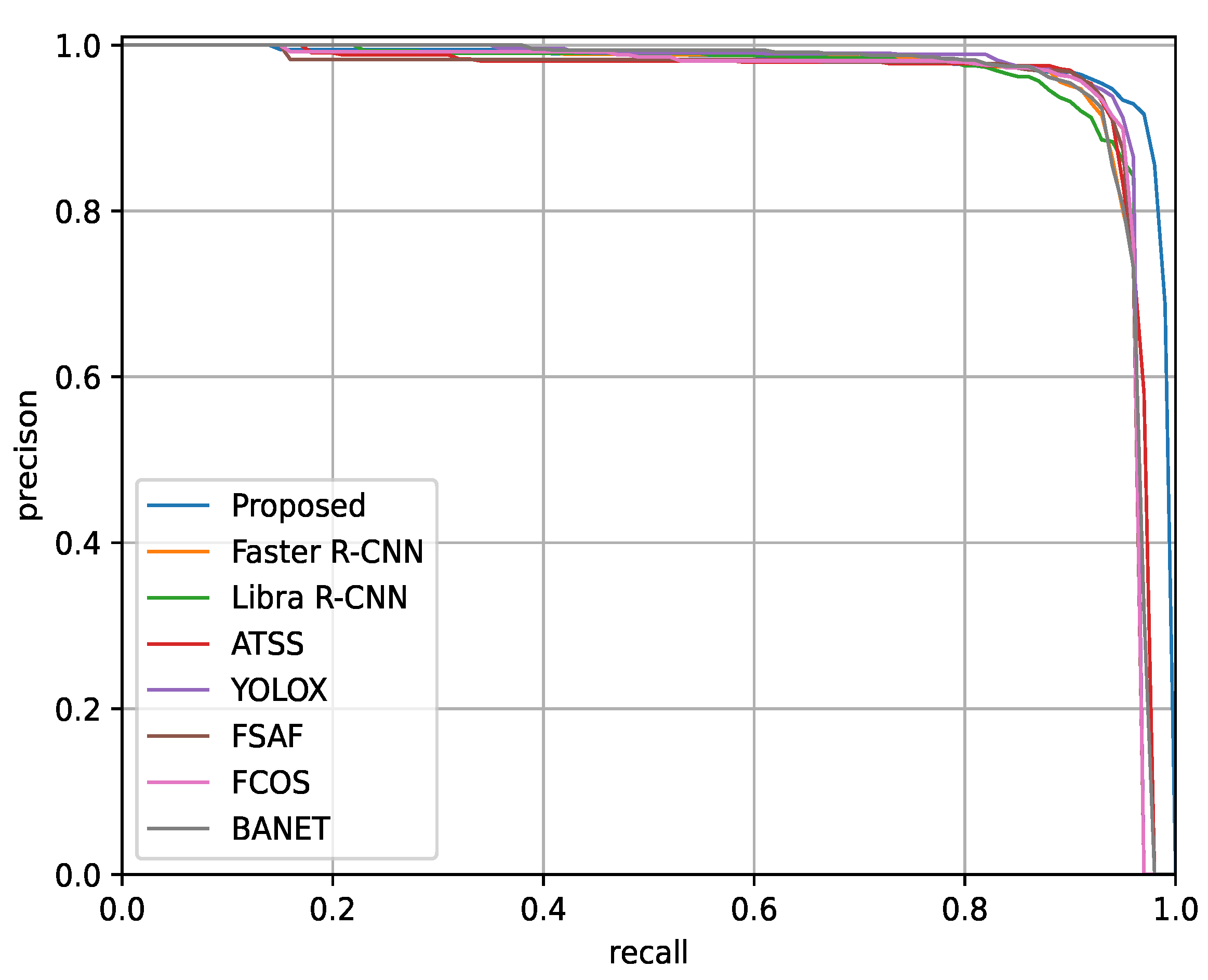
3.5.1. Experimental Results on SSDD

The experimental results on SSDD are listed in Table 2. In terms of YOLOX, other indicators except A P l are inferior to those of the proposed method. In particular, A P 50 of the proposed method is 2.2% higher than that of YOLOX. It is gratifying that the detection performance of the proposed method is also much better than that of two-stage detection methods, namely Faster R-CNN and Libra R-CNN. It can be seen from Table 2 that the proposed method is superior to all competitors. Moreover, the corresponding PR curve of each method is presented to reveal the effectiveness of the proposed method from another perspective, as depicted in Figure 9. One can see that the area under the curve corresponding to the proposed method is the largest among all methods, which further reveals that the proposed method has outstanding detection performance.

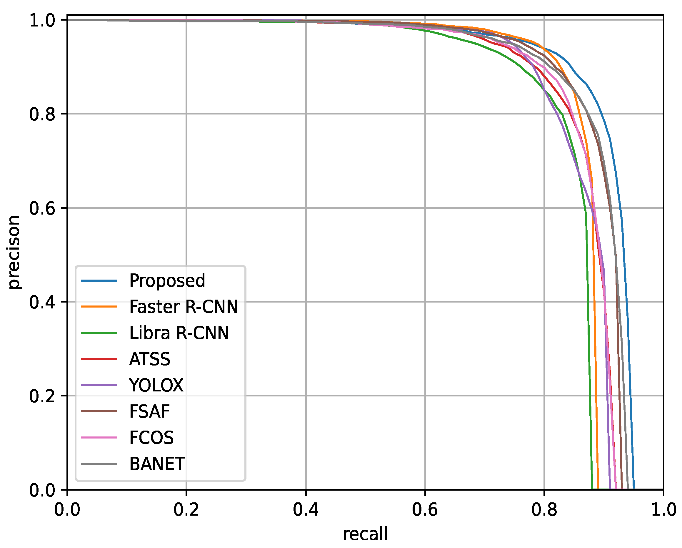
3.5.2. Experimental Results on HRSID

The experimental results on HRSID are given in Table 3. Apparently, it can be seen from Table 3 that each evaluation indicator of each method decreases to varying degrees on HRSID compared with the experimental results on SSDD. One main reason for this phenomenon is that in the publicly released HRSID, there are more complex SAR scenes with multiple resolutions and polarization modes, complex sea states, and more coastal ports.
As can be seen from Table 3, the evaluation indicators of the proposed method are the best among all methods. Especially for multi-scale ship detection, the A P s , A P m , and A P l of the proposed method can reach 68.0%, 68.9%, 33.3%, respectively, which are 1.8%, 3.9%, and 16.4% higher than the best indicators among all competitors. Figure 10 plots the PR curve of each method. From the experimental results in Figure 10, one can see that the area under the curve corresponding to the proposed method is larger than that of any comparison method, indicating that the proposed method can obtain optimal detection performance. Based on these convincing experimental results, it follows that the proposed method is significantly competitive for multi-scale ship object detection in complex SAR scenes.

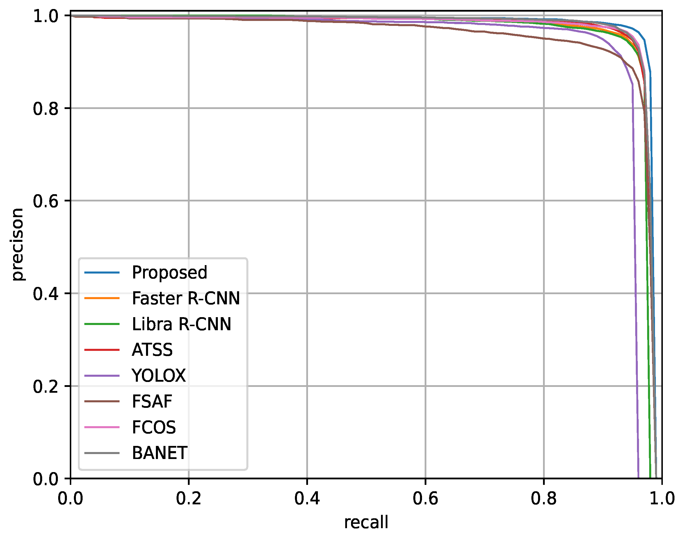
3.5.3. Experimental Results on the SAR-Ship-Dataset

Evaluation experiments are conducted on the SAR-Ship-Dataset to investigate the generalization of the proposed method. The experimental results are listed in Table 4.
First, it can be easily observed that the proposed method outperforms the two-stage detection methods, i.e., Faster R-CNN and Libra R-CNN in all aspects of performance. Second, one can see that the F1 score of the proposed method is higher than that of each one-stage detection method. For multi-scale ship object detection, the proposed method appears to have significant advantages in large scenes, especially for small-scale and middle-scale ship object detection. From a quantitative point of view, A P s and A P m of the proposed method are 2.6% and 4% higher than those of the best indicators among all competitors, respectively. In terms of large-scale object detection, the performance of the proposed method is better than or comparable to that of each competitor. Likewise, the PR curve of each method is plotted in Figure 11. One can see from Figure 11 that the area under the curve corresponding to the proposed method is still the largest. In view of the above qualitative and quantitative results and analysis, it can be inferred that the proposed method has a powerful generalization ability in SAR ship object detection tasks.
From the experimental results on three SAR datasets, it can be seen that the proposed method is the best compared to all competitors in terms of detection accuracy, but its complexity and inference time are slightly inferior to each comparison method. In fact, we all know that this experimental phenomenon is expected. How to strike a balance between model complexity and accuracy is a topic to be discussed in future work.

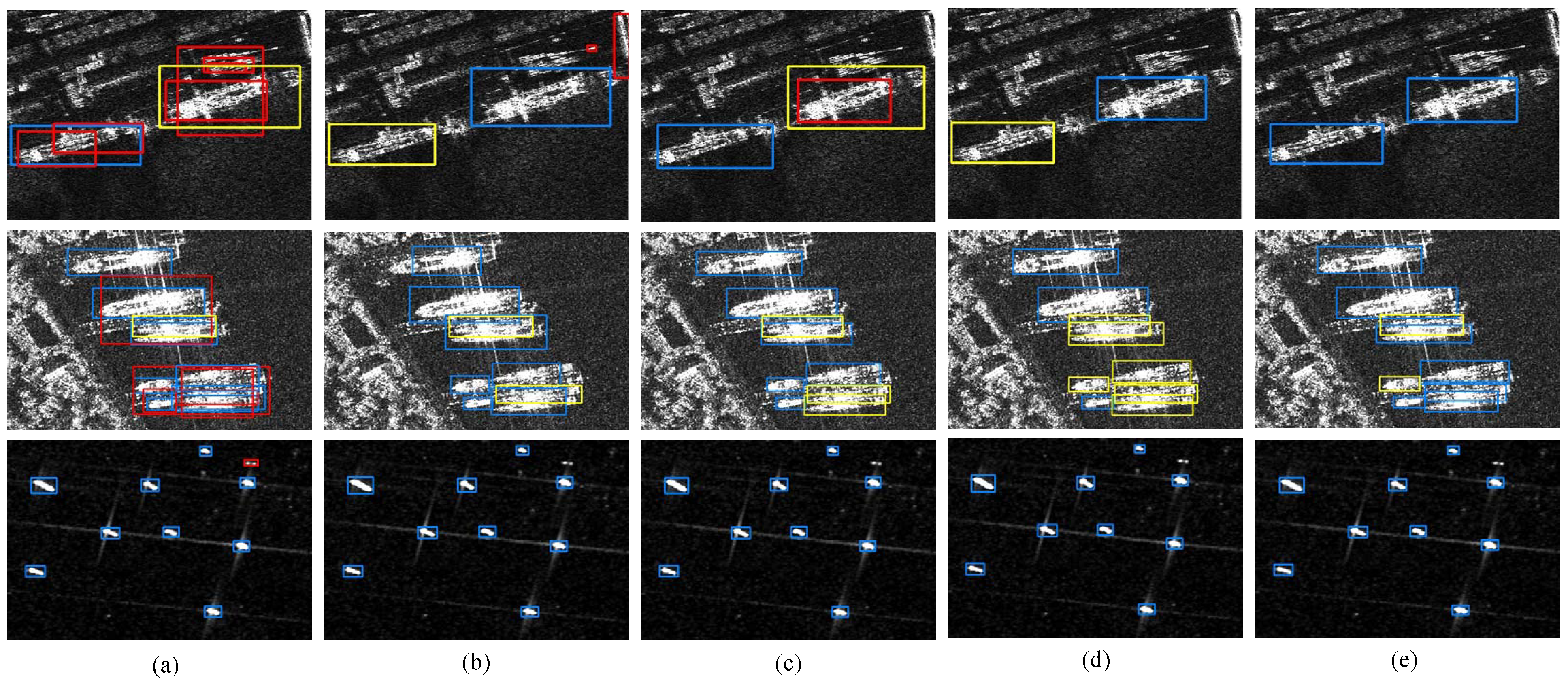
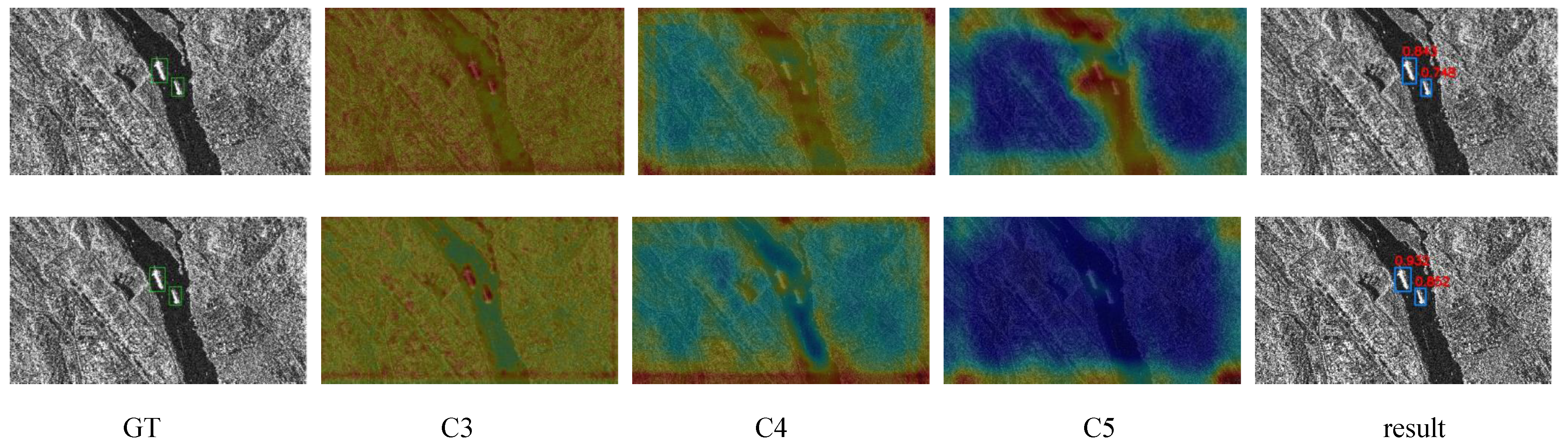
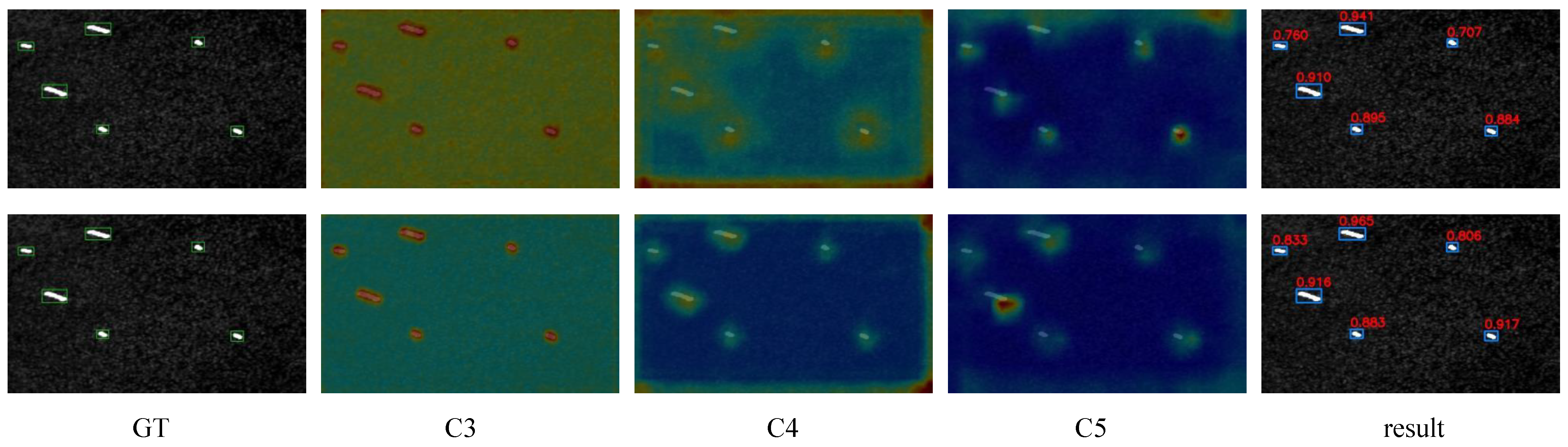
3.6. Visual Results and Analysis

To further demonstrate the effectiveness of the proposed method, the detection results obtained on three datasets are shown in Figure 12, Figure 13 and Figure 14, in which the blue box, yellow box, and red box indicate the correct detection result, the missed detection result, and the false alarm, respectively. Due to space constraints, this section only presents the detection results of Faster R-CNN, YOLOX, ATSS, FCOS, and our method in different scenarios.
Figure 12 shows the detection results of each method on SSDD, where the detection results of inshore ships, densely arranged ships, and offshore ships are shown, respectively. From the visual results in Figure 12, one can see that both FCOS and ATSS appear the missed detection, while YOLOX and Faster R-CNN fail to thoroughly suppress land interference, resulting in a higher false alarm rate in inshore scenes. The number of ATSS and FCOS missed ships is relatively high. Faster R-CNN has a low missed rate but a high error rate, while YOLOX is comparable to the proposed method in densely arranged scenes. In offshore scenes, all methods except Faster R-CNN perform satisfactorily.
Figure 13 displays the ship-detection results of the river ships, inshore ships, and offshore ships on HRSID. It can be observed that in the river scenes, YOLOX and Faster R-CNN have more false alarm ships, while ATSS and FCOS have more missed detection ships. In inshore scenes, the number of missed ships using the proposed method is the lowest compared with competitors. Moreover, one can see that the number of missed ships using the proposed method is less than that of FCOS and ATSS, which is comparable to that of Faster R-CNN in offshore scenes.
The experimental results on the SAR-Ship-Dataset are shown in Figure 14, where ship-detection results in inshore, offshore, and complex interference scenarios are presented. From Figure 14, one can see that ATSS and FCOS occur in the phenomenon of missed detection. Faster R-CNN has more false alarms for small-scale ships, and YOLOX performs poorly in complex scenes. In contrast, whether there are false alarms or missed detection, the proposed method is the least among competitors.
The above qualitative experimental results in various scenes further manifest the advantages and potential of the proposed anchor-free detection method in SAR ship detection tasks.

4. Conclusions

In this article, a novel SAR ship detection method named multi-level feature-refinement anchor-free framework with consistent label-assignment mechanism is proposed. The novelties of this article can be summarized into three aspects. First, a stepwise feature-refinement backbone network is developed to refine the position and contour of the ship object, therefore highlighting ship features while suppressing complex background clutter interference. Second, an adjacent feature-refined pyramid network is devised to alleviate multi-scale high-level semantic loss and enhance low-level positioning information, which is very beneficial to multi-scale ship object detection. Third, a new label-assignment method based on consistent feature scale constraints, dubbed a consistent label-assignment mechanism, is proposed to assign labels to the samples rationally, which can boost the detection accuracy of ship objects, especially for densely arranged ships. Experimental results show that the proposed method outperforms all competitors, and the AP of the proposed method on SSDD, HRSID, and SAR-Ship-Dataset is 0.8%, 3.6%, 3.8% higher than that of the best competitor, respectively.

Author Contributions

Conceptualization, Y.Z.; methodology, Y.Z. and S.W.; software, Y.Z. and L.Z.; validation, Y.Z., S.W., H.R. and X.W.; formal analysis, Y.Z.; investigation, Y.Z. and L.Z.; resources, H.R.; data curation, S.W. and J.H.; writing—original draft preparation, Y.Z.; writing—review and editing, S.W. and H.R.; visualization, S.W. and J.H.; supervision, H.R.; project administration, X.W.; funding acquisition, X.W. and H.R. All authors have read and agreed to the published version of the manuscript.

Funding

This research was supported by the National Science Foundation of China (Grant 42027805 and 62201124).

Data Availability Statement

Data are contained within the article.

Conflicts of Interest

The authors declare no conflicts of interest.

References

  1. Robey, F.C.; Fuhrmann, D.R.; Kelly, E.J.; Nitzberg, R. A CFAR adaptive matched filter detector. IEEE Trans. Aerosp. Electron. Syst. 1992, 28, 208–216. [Google Scholar] [CrossRef]
  2. Conte, E.; De Maio, A.; Ricci, G. Recursive estimation of the covariance matrix of a compound-Gaussian process and its application to adaptive CFAR detection. IEEE Trans. Signal Process. 2002, 50, 1908–1915. [Google Scholar] [CrossRef]
  3. Lei, S.; Zhao, Z.; Nie, Z.; Liu, Q.H. A CFAR adaptive subspace detector based on a single observation in system-dependent clutter background. IEEE Trans. Signal Process. 2014, 62, 5260–5269. [Google Scholar] [CrossRef]
  4. Dai, H.; Du, L.; Wang, Y.; Wang, Z. A modified CFAR algorithm based on object proposals for ship target detection in SAR images. IEEE Geosci. Remote Sens. Lett. 2016, 13, 1925–1929. [Google Scholar] [CrossRef]
  5. Qin, X.; Zhou, S.; Zou, H.; Gao, G. A CFAR detection algorithm for generalized gamma distributed background in high-resolution SAR images. IEEE Geosci. Remote Sens. Lett. 2012, 10, 806–810. [Google Scholar]
  6. Pappas, O.; Achim, A.; Bull, D. Superpixel-level CFAR detectors for ship detection in SAR imagery. IEEE Geosci. Remote Sens. Lett. 2018, 15, 1397–1401. [Google Scholar] [CrossRef]
  7. Gao, G.; Shi, G. CFAR ship detection in nonhomogeneous sea clutter using polarimetric SAR data based on the notch filter. IEEE Trans. Geosci. Remote Sens. 2017, 55, 4811–4824. [Google Scholar] [CrossRef]
  8. Girshick, R.; Donahue, J.; Darrell, T.; Malik, J. Rich feature hierarchies for accurate object detection and semantic segmentation. In Proceedings of the IEEE Conference on Computer Vision and Pattern Recognition, Columbus, OH, USA, 23–28 June 2014; pp. 580–587. [Google Scholar]
  9. Lee, H.; Eum, S.; Kwon, H. Me r-cnn: Multi-expert r-cnn for object detection. IEEE Trans. Image Process. 2019, 29, 1030–1044. [Google Scholar] [CrossRef]
  10. Yang, L.; Song, Q.; Wang, Z.; Hu, M.; Liu, C. Hier R-CNN: Instance-level human parts detection and a new benchmark. IEEE Trans. Image Process. 2020, 30, 39–54. [Google Scholar] [CrossRef]
  11. Ren, S.; He, K.; Girshick, R.; Sun, J. Faster r-cnn: Towards real-time object detection with region proposal networks. Adv. Neural Inf. Process. Syst. 2015, 28, 1137–1149. [Google Scholar] [CrossRef]
  12. Pang, J.; Chen, K.; Shi, J.; Feng, H.; Ouyang, W.; Lin, D. Libra r-cnn: Towards balanced learning for object detection. In Proceedings of the IEEE/CVF Conference on Computer Vision and Pattern Recognition, Long Beach, CA, USA, 15–20 June 2019; pp. 821–830. [Google Scholar]
  13. Lin, T.Y.; Goyal, P.; Girshick, R.; He, K.; Dollár, P. Focal loss for dense object detection. In Proceedings of the IEEE International Conference on Computer Vision, Venice, Italy, 22–29 October 2017; pp. 2980–2988. [Google Scholar]
  14. Redmon, J.; Divvala, S.; Girshick, R.; Farhadi, A. You only look once: Unified, real-time object detection. In Proceedings of the IEEE Conference on Computer Vision and Pattern Recognition, Las Vegas, NV, USA, 27–30 June 2016; pp. 779–788. [Google Scholar]
  15. Redmon, J.; Farhadi, A. YOLO9000: Better, faster, stronger. In Proceedings of the IEEE Conference on Computer Vision and Pattern Recognition, Honolulu, HI, USA, 21–26 July 2017; pp. 7263–7271. [Google Scholar]
  16. Yu, N.; Ren, H.; Deng, T.; Fan, X. A Lightweight Radar Ship Detection Framework with Hybrid Attentions. Remote Sens. 2023, 15, 2743. [Google Scholar] [CrossRef]
  17. Liu, W.; Anguelov, D.; Erhan, D.; Szegedy, C.; Reed, S.; Fu, C.Y.; Berg, A.C. Ssd: Single shot multibox detector. In Proceedings of the Computer Vision–ECCV 2016: 14th European Conference, Amsterdam, The Netherlands, 11–14 October 2016; Springer: Berlin/Heidelberg, Germany, 2016; pp. 21–37. [Google Scholar]
  18. Zhang, H.; Tian, Y.; Wang, K.; Zhang, W.; Wang, F.Y. Mask SSD: An effective single-stage approach to object instance segmentation. IEEE Trans. Image Process. 2019, 29, 2078–2093. [Google Scholar] [CrossRef]
  19. Tian, Z.; Shen, C.; Chen, H.; He, T. Fcos: Fully convolutional one-stage object detection. In Proceedings of the Proceedings of the IEEE/CVF International Conference on Computer Vision, Seoul, Republic of Korea, 27 October–2 November 2019; pp. 9627–9636. [Google Scholar]
  20. Ge, Z.; Liu, S.; Wang, F.; Li, Z.; Sun, J. Yolox: Exceeding YOLO series in 2021. arXiv 2021, arXiv:2107.08430. [Google Scholar]
  21. Zhang, S.; Chi, C.; Yao, Y.; Lei, Z.; Li, S.Z. Bridging the gap between anchor-based and anchor-free detection via adaptive training sample selection. In Proceedings of the IEEE/CVF Conference on Computer Vision and Pattern Recognition, Seattle, WA, USA, 13–19 June 2020; pp. 9759–9768. [Google Scholar]
  22. Zhu, C.; He, Y.; Savvides, M. Feature selective anchor-free module for single-shot object detection. In Proceedings of the IEEE/CVF Conference on Computer Vision and Pattern Recognition, Long Beach, CA, USA, 15–20 June 2019; pp. 840–849. [Google Scholar]
  23. Shi, H.; Fang, Z.; Wang, Y.; Chen, L. An adaptive sample assignment strategy based on feature enhancement for ship detection in SAR images. Remote Sens. 2022, 14, 2238. [Google Scholar] [CrossRef]
  24. Yao, C.; Xie, P.; Zhang, L.; Fang, Y. ATSD: Anchor-Free Two-Stage Ship Detection Based on Feature Enhancement in SAR Images. Remote Sens. 2022, 14, 6058. [Google Scholar] [CrossRef]
  25. Wang, J.; Cui, Z.; Jiang, T.; Cao, C.; Cao, Z. Lightweight Deep Neural Networks for Ship Target Detection in SAR Imagery. IEEE Trans. Image Process. 2022, 32, 565–579. [Google Scholar] [CrossRef]
  26. Wang, Z.; Wang, R.; Ai, J.; Zou, H.; Li, J. Global and Local Context-Aware Ship Detector for High-Resolution SAR Images. IEEE Trans. Aerosp. Electron. Syst. 2023, 59, 4159–4167. [Google Scholar] [CrossRef]
  27. Zhang, T.; Zeng, T.; Zhang, X. Synthetic aperture radar (SAR) meets deep learning. Remote Sens. 2023, 15, 303. [Google Scholar] [CrossRef]
  28. Cui, Z.; Li, Q.; Cao, Z.; Liu, N. Dense attention pyramid networks for multi-scale ship detection in SAR images. IEEE Trans. Geosci. Remote Sens. 2019, 57, 8983–8997. [Google Scholar] [CrossRef]
  29. Duan, K.; Bai, S.; Xie, L.; Qi, H.; Huang, Q.; Tian, Q. Centernet: Keypoint triplets for object detection. In Proceedings of the IEEE/CVF International Conference on Computer Vision and Pattern Recognition, Long Beach, CA, USA, 15–20 June 2019; pp. 6569–6578. [Google Scholar]
  30. Guo, H.; Yang, X.; Wang, N.; Gao, X. A CenterNet++ model for ship detection in SAR images. Pattern Recognit. 2021, 112, 107787. [Google Scholar] [CrossRef]
  31. Sun, Z.; Dai, M.; Leng, X.; Lei, Y.; Xiong, B.; Ji, K.; Kuang, G. An anchor-free detection method for ship targets in high-resolution SAR images. IEEE J. Sel. Top. Appl. Earth Obs. Remote Sens. 2021, 14, 7799–7816. [Google Scholar] [CrossRef]
  32. Wan, H.; Chen, J.; Huang, Z.; Xia, R.; Wu, B.; Sun, L.; Yao, B.; Liu, X.; Xing, M. AFSar: An anchor-free SAR target detection algorithm based on multiscale enhancement representation learning. IEEE Trans. Geosci. Remote Sens. 2021, 60, 5219514. [Google Scholar] [CrossRef]
  33. Hu, Q.; Hu, S.; Liu, S. BANet: A balance attention network for anchor-free ship detection in SAR images. IEEE Trans. Geosci. Remote Sens. 2022, 60, 5222212. [Google Scholar] [CrossRef]
  34. Li, J.; Xu, C.; Su, H.; Gao, L.; Wang, T. Deep learning for SAR ship detection: Past, present and future. Remote Sens. 2022, 14, 2712. [Google Scholar] [CrossRef]
  35. Li, J.; Chen, J.; Cheng, P.; Yu, Z.; Yu, L.; Chi, C. A Survey on Deep-Learning-Based Real-Time SAR Ship Detection. IEEE J. Sel. Top. Appl. Earth Obs. Remote Sens. 2023, 16, 3218–3247. [Google Scholar] [CrossRef]
  36. Yang, X.; Zhang, X.; Wang, N.; Gao, X. A robust one-stage detector for multiscale ship detection with complex background in massive SAR images. IEEE Trans. Geosci. Remote Sens. 2021, 60, 5217712. [Google Scholar] [CrossRef]
  37. Woo, S.; Park, J.; Lee, J.Y.; Kweon, I.S. Cbam: Convolutional block attention module. In Proceedings of the European Conference on Computer Vision (ECCV), Munich, Germany, 8–14 September 2018; pp. 3–19. [Google Scholar]
  38. Hou, Q.; Zhou, D.; Feng, J. Coordinate attention for efficient mobile network design. In Proceedings of the IEEE/CVF Conference on Computer Vision and Pattern Recognition, Nashville, TN, USA, 20–25 June 2021; pp. 13713–13722. [Google Scholar]
  39. Lin, T.Y.; Dollár, P.; Girshick, R.; He, K.; Hariharan, B.; Belongie, S. Feature pyramid networks for object detection. In Proceedings of the IEEE Conference on Computer Vision and Pattern Recognition, Honolulu, HI, USA, 21–26 July 2017; pp. 2117–2125. [Google Scholar]
  40. Shi, W.; Caballero, J.; Huszár, F.; Totz, J.; Aitken, A.P.; Bishop, R.; Rueckert, D.; Wang, Z. Real-time single image and video super-resolution using an efficient sub-pixel convolutional neural network. In Proceedings of the IEEE Conference on Computer Vision and Pattern Recognition, Las Vegas, NV, USA, 7–30 June 2016; pp. 1874–1883. [Google Scholar]
  41. Hu, J.; Shen, L.; Sun, G. Squeeze-and-excitation networks. In Proceedings of the Proceedings of the IEEE Conference on Computer Vision and Pattern Recognition, Salt Lake City, UT, USA, 8–22 June 2018; pp. 7132–7141. [Google Scholar]
  42. Luo, Y.; Cao, X.; Zhang, J.; Guo, J.; Shen, H.; Wang, T.; Feng, Q. CE-FPN: Enhancing channel information for object detection. Multimed. Tools Appl. 2022, 81, 30685–30704. [Google Scholar] [CrossRef]
  43. Rezatofighi, H.; Tsoi, N.; Gwak, J.; Sadeghian, A.; Reid, I.; Savarese, S. Generalized intersection over union: A metric and a loss for bounding box regression. In Proceedings of the IEEE/CVF Conference on Computer Vision and Pattern Recognition, Long Beach, CA, USA, 15–20 June 2019; pp. 658–666. [Google Scholar]
  44. Li, J.; Qu, C.; Shao, J. Ship detection in SAR images based on an improved faster R-CNN. In Proceedings of the 2017 SAR in Big Data Era: Models, Methods and Applications (BIGSARDATA), Beijing, China, 13–14 November 2017; pp. 1–6. [Google Scholar]
  45. Wei, S.; Zeng, X.; Qu, Q.; Wang, M.; Su, H.; Shi, J. HRSID: A high-resolution SAR images dataset for ship detection and instance segmentation. IEEE Access 2020, 8, 120234–120254. [Google Scholar] [CrossRef]
  46. Wang, Y.; Wang, C.; Zhang, H.; Dong, Y.; Wei, S. A SAR dataset of ship detection for deep learning under complex backgrounds. Remote Sens. 2019, 11, 765. [Google Scholar] [CrossRef]
  47. Zhang, T.; Zhang, X.; Li, J.; Xu, X.; Wang, B.; Zhan, X.; Xu, Y.; Ke, X.; Zeng, T.; Su, H.; et al. SAR ship detection dataset (SSDD): Official release and comprehensive data analysis. Remote Sens. 2021, 13, 3690. [Google Scholar] [CrossRef]
  48. Zhang, T.; Zhang, X.; Ke, X. Quad-FPN: A novel quad feature pyramid network for SAR ship detection. Remote Sens. 2021, 13, 2771. [Google Scholar] [CrossRef]
Figure 1. Framework of the proposed method.
Remotesensing 16 00975 g001
Figure 2. Stepwise feature refinement backbone network architecture.
Remotesensing 16 00975 g002
Figure 3. Network architecture of sup-pixel sampling-based adjacent feature fusion.
Remotesensing 16 00975 g003
Figure 4. Consistent Label-Assignment Mechanism.
Remotesensing 16 00975 g004
Figure 5. The output features of the backbone network in different feature layers and IoU scores with GT box (In inshore scene).
Remotesensing 16 00975 g005
Figure 6. The output features of the backbone network in different feature layers and IoU scores with GT box (In river scene).
Remotesensing 16 00975 g006
Figure 7. The output features of the backbone network in different feature layers and IoU scores with GT box (In offshore scene).
Remotesensing 16 00975 g007
Figure 8. Visual results of sample label assignment in different feature layers.
Remotesensing 16 00975 g008
Figure 9. PR curve of each method on SSDD.
Remotesensing 16 00975 g009
Figure 10. PR curve of each method on HRSID.
Remotesensing 16 00975 g010
Figure 11. PR curve of each method on SAR-Ship-Dataset.
Remotesensing 16 00975 g011
Figure 12. Visualization results of ship detection for each method in different SSDD scenarios. (a) Faster R-CNN, (b) YOLOX, (c) ATSS, (d) FCOS, (e) Our method.
Remotesensing 16 00975 g012
Figure 13. Visualization results of ship detection for each method in different scenarios on HRSID. (a) Faster R-CNN, (b) YOLOX, (c) ATSS, (d) FCOS, (e) Our method.
Remotesensing 16 00975 g013
Figure 14. Visualization results of ship detection for each method in different scenarios on SAR-Ship-Dataset. (a) Faster R-CNN, (b) YOLOX, (c) ATSS, (d) FCOS, (e) Our method.
Remotesensing 16 00975 g014
Table 1. Ablation Experiments.
SwFRAFRPNCLAMPRF1AP AP 50 AP 75 AP s AP m AP l
baseline×××93.992.593.258.994.367.255.165.357.4
model1××94.294.094.159.895.269.855.567.058.6
model2×95.093.294.161.396.069.755.969.562.1
model395.194.094.562.097.271.258.367.665.7
Table 2. Performance Comparison of Different Methods on SSDD.
MethodBackbonePRF1AP AP 50 AP 75 AP s AP m AP l Params (M)FLOPs (G)FPS
Faster R-CNN [11]ResNet-10194.990.892.859.694.469.955.865.760.460.1141.647.2
Libra R-CNN [12]ResNet-10191.991.691.760.394.269.756.267.061.660.4142.145.5
ATSS [21]ResNet-10195.091.993.458.494.665.052.967.060.450.9131.947.4
YOLOX [20]CSPDarknet-5394.293.894.061.295.069.657.366.867.254.292.267.1
FSAF [22]ResNet-10195.192.093.556.694.065.052.663.458.455.0132.347.7
FCOS [19]ResNet-10193.992.593.258.994.367.255.165.357.450.8129.648.8
BANet [33]ResNet-10193.991.992.958.794.967.355.464.954.363.9147.035.2
ProposedSwFR95.194.094.562.097.271.258.367.665.758.7167.236.1
Table 3. Performance Comparison of Different Methods on HRSID.
MethodBackbonePRF1AP AP 50 AP 75 AP s AP m AP l Params (M)FLOPs (G)FPS
Faster R-CNN [11]ResNet-10191.782.086.562.286.171.463.363.814.260.1289.226.2
Libra R-CNN [12]ResNet-10187.478.482.760.383.768.261.363.210.560.4290.326.1
ATSS [21]ResNet-10189.978.784.061.586.368.862.665.016.950.9284.126.2
YOLOX [20]CSPDarknet-5390.877.883.862.885.871.966.251.81.754.2198.835.9
FSAF [22]ResNet-10189.082.985.861.588.669.462.263.813.555.0285.026.7
FCOS [19]ResNet-10189.580.384.760.786.467.662.061.614.750.8279.226.5
BANet [33]ResNet-10189.182.085.453.688.762.055.353.112.463.9302.019.0
ProposedSwFR92.283.987.366.490.375.468.068.933.358.7360.219.5
Table 4. Performance Comparison of Different Methods on SAR-Ship-Dataset.
MethodBackbonePRF1AP AP 50 AP 75 AP s AP m AP l Params (M)FLOPs (G)FPS
Faster R-CNN [11]ResNet-10194.993.794.361.496.071.156.467.851.660.182.768.4
Libra R-CNN [12]ResNet-10194.694.194.363.795.975.058.470.153.360.483.066.7
ATSS [21]ResNet-10195.294.794.963.896.574.558.571.164.850.971.070.9
YOLOX [20]CSPDarknet-5394.690.592.556.893.462.151.364.343.254.249.7102.8
FSAF [22]ResNet-10191.192.991.959.594.866.954.765.762.255.071.371.4
FCOS [19]ResNet-10195.595.095.263.296.674.657.970.564.150.869.873.4
BANet [33]ResNet-10196.294.295.262.996.972.457.270.260.263.979.252.0
ProposedSwFR96.296.296.267.697.380.561.175.164.958.790.153.8
Disclaimer/Publisher’s Note: The statements, opinions and data contained in all publications are solely those of the individual author(s) and contributor(s) and not of MDPI and/or the editor(s). MDPI and/or the editor(s) disclaim responsibility for any injury to people or property resulting from any ideas, methods, instructions or products referred to in the content.

