Abstract
Clouds often cause challenges during the application of optical satellite images. Masking clouds and cloud shadows is a crucial step in the image preprocessing workflow. The absence of a thermal band in products of the Sentinel-2 series complicates cloud detection. Additionally, most existing cloud detection methods provide binary results (cloud or non-cloud), which lack information on thin clouds and cloud shadows. This study attempted to use end-to-end supervised spatial–temporal deep learning (STDL) models to enhance cloud detection in Sentinel-2 imagery for China. To support this workflow, a new dataset for time-series cloud detection featuring high-quality labels for thin clouds and haze was constructed through time-series interpretation. A classification system consisting of six categories was employed to obtain more detailed results and reduce intra-class variance. Considering the balance of accuracy and computational efficiency, we constructed four STDL models based on shared-weight convolution modules and different classification modules (dense, long short-term memory (LSTM), bidirectional LSTM (Bi-LSTM), and transformer). The results indicated that spatial and temporal features were crucial for high-quality cloud detection. The STDL models with simple architectures that were trained on our dataset achieved excellent accuracy performance and detailed detection of clouds and cloud shadows, although only four bands with a resolution of 10 m were used. The STDL models that used the Bi-LSTM and that used the transformer as the classifier showed high and close overall accuracies. While the transformer classifier exhibited slightly lower accuracy than that of Bi-LSTM, it offered greater computational efficiency. Comparative experiments also demonstrated that the usable data labels and cloud detection results obtained with our workflow outperformed the results of the existing s2cloudless, MAJA, and CS+ methods.
1. Introduction
The explosion of remote sensing data and the advent of large-scale cloud computing have significantly advanced scientific discoveries across various fields [1,2,3,4]. A pivotal catalyst in these advancements lies in the ability of optical satellite sensors to trace the physical properties of land with higher spatial resolution and at shorter temporal intervals. Nonetheless, a substantial challenge arises from the inherent limitations of optical sensors, resulting in the inevitable contamination of most images by clouds and raising biases during the analysis of imagery. Thus, to mitigate biases during the analysis of remote sensing imagery, the development of automated, accurate, and efficient methods for cloud and cloud shadow detection is crucial, especially in the context of the preprocessing of large-scale remote sensing data. Sentinel-2 satellite imagery provides valuable datasets with a wide swath width, high spatial resolution, and frequent revisit times. It includes bands across the visible, near-infrared, and shortwave infrared ranges. However, cloud detection in Sentinel-2 imagery remains a significant challenge due to the lack of a thermal band [5].
Various cloud and cloud shadow detection algorithms have been developed for Sentinel-2 images, and they can be broadly classified into physical-rule-based algorithms, multi-temporal-based algorithms, and machine-learning-based algorithms.
Physical-rule-based algorithms are designed based on the large gaps in spectral and spatial characteristics between clouds and ground objects, and the cloud and cloud shadow masks can be obtained by setting thresholds according to the single-band reflectance, band ratios, and differences [6,7]. These methods are simple and effective for the screening of typical clouds and cloud shadows in simple scenes. They can directly operate on an image without relying on sample data and additional auxiliary data. However, their reliance on empirically determined parameters and sensitivity to parameter selection can lead to the omission of thin clouds and the inclusion of bright, non-cloud objects (e.g., snow). Temporal and spatial variations further make it more difficult to find suitable thresholds.
Multi-temporal algorithms typically use cloud-free images/pixels as a reference and mark pixels with significant differences in reflectance from the reference images as potential cloud or cloud shadow pixels [8,9,10]. In addition, cloud effects can also be obtained by comparing the original values with the predicted values of a time-series change trend model fitted with non-cloud pixels, which requires an initial cloud mask [11,12,13]. The 5-day revisit period and free availability of Sentinel-2 imagery facilitate the development of multi-temporal cloud detection algorithms. In comparison with single-temporal cloud detection algorithms, multi-temporal algorithms leverage temporal information to complement physical properties, and they can better distinguish cloud effects and ground objects [14]. However, their accuracy performance can be limited by the reference image, initial cloud mask, and real land-cover changes.
Machine-learning-based algorithms, including traditional machine learning methods and deep learning methods, treat cloud and cloud shadow detection as a classification problem by optimizing the parameters of the designed model based on a mass of representative training data [15]. The success of machine-learning-based methods relies on the availability of a large number of labeled samples, and many cloud detection datasets have been published [16,17,18]. Traditional machine learning methods, such as the support vector machine (SVM) [19], random forest [20], classical Bayesian [17], fuzzy clustering [21], boosting [22], and neural networks [23], have achieved significant results in cloud detection. Compared to non-machine learning methods, these approaches can automatically uncover complex nonlinear relationships between different patterns while also achieving end-to-end rapid data processing. However, traditional machine-learning-based approaches, together with the above physical-rule-based and multi-temporal algorithms, usually rely on manual feature selection and use limited information on the spatial context; thus, they cannot effectively deal with cloud and cloud shadow detection in complex scenes.
Recently, deep learning methods have been increasingly used in cloud detection, and they have achieved outstanding performance [24,25,26,27]. Deep-learning-based algorithms automatically learn spatial and semantic features directly from training data, avoiding the need for manual feature selection and reducing the reliance on subjective experience. Inspired by state-of-the-art deep learning architectures, such as U-Net [28], DeepLab v3+ [29], and ResNet [30], many cloud detection models have been proposed [16]. Techniques such as weakly supervised learning and domain adaptation have also been developed to address the challenge of insufficient labeled data in cloud detection [31,32,33,34]. Deep learning methods can automatically learn high-level feature representations of data, avoiding the need for manual feature engineering. These algorithms are able to achieve more accurate results in complex scenes, such as in snow/ice-covered areas and urban areas. However, deep-learning-based methods still rely heavily on representative training data, which may not be available in sufficient quantities, especially for thin clouds and cloud shadows. In fact, these two types are difficult to define in a single scene.
Although a number of cloud detection algorithms are currently available for Sentinel-2 imagery, a comparison of their results shows that the performance of these methods varies depending on the reference dataset, and no algorithm has been able to achieve both production accuracy and user accuracy greater than 90% [5]. Google introduced the Cloud Score+ (CS+) method just a few months ago [34]. This method skips cloud detection and employs a weakly supervised method to directly quantify the availability of data. CS+ performs better than existing methods at masking unavailable data, such as clouds and cloud shadows, but it still relies on manual trade-offs between inclusions and omissions, and it misses the boundaries among clouds, thin clouds, and cloud shadows. In general, an accurate and detailed cloud and cloud shadow mask for Sentinel-2 imagery remains elusive.
This study attempted to employ end-to-end spatial–temporal deep learning models to achieve high-quality cloud detection. The combination of spectral, spatial, and temporal features was expected to improve the results, especially for thin clouds and cloud shadows. We employed a classification system consisting of six categories to obtain more detailed cloud and cloud shadow detection results while reducing intra-class variance and simplifying the pattern complexity. Additionally, by utilizing dense time-series Sentinel-2 data, based on the six-class classification system, we constructed a time-series cloud detection dataset distributed across mainland China. This dataset can serve to support the construction and validation of time-series models.
2. Materials and Methods
This study focused on producing finer cloud and cloud shadow masks of Sentinel-2 imagery across mainland China. Spatial–temporal deep learning (STDL) architectures were tested for the task of series image classification. We also developed a new time-series dataset to support data-driven deep learning methods.
2.1. Satellite Data
We employed the Sentinel-2 Level-1C (L1C) product in this work to build the time-series cloud detection dataset, which contains rich temporal and spatial information. The Sentinel-2 mission consists of two satellites, making the revisit period short; it is 5 days with the two satellites at the equator and 2–3 days at mid-latitudes. The L1C product provides the scaled top-of-atmosphere (TOA) reflectance of 13 spectral bands, and the digital number (DN) value is the reflectance multiplied by 10,000. There are four bands with a resolution of 10 m (B2, B3, B4, and B8), six bands with a resolution of 20 m, and three bands with a resolution of 60 m. The details of the band definitions can be seen in Table 1. In addition, the Sentinel-2 L1C product also contains a true-color image (TCI), which is a composite of B4 (red), B3 (green), and B2 (blue). The TOA reflectance values from 0 to 0.3558 were rescaled to a range from 1 to 255 in TCI.

Table 1.
Band definitions in Sentinel-2 imagery. Data source: https://gdal.org/drivers/raster/sentinel2.html (accessed on 4 February 2024).
It is worth noting that the DN values were shifted by 1000 in PROCESSING_BASELINE ‘04.00’ or above after 25 January 2022. These shifted values were corrected during our data processing.
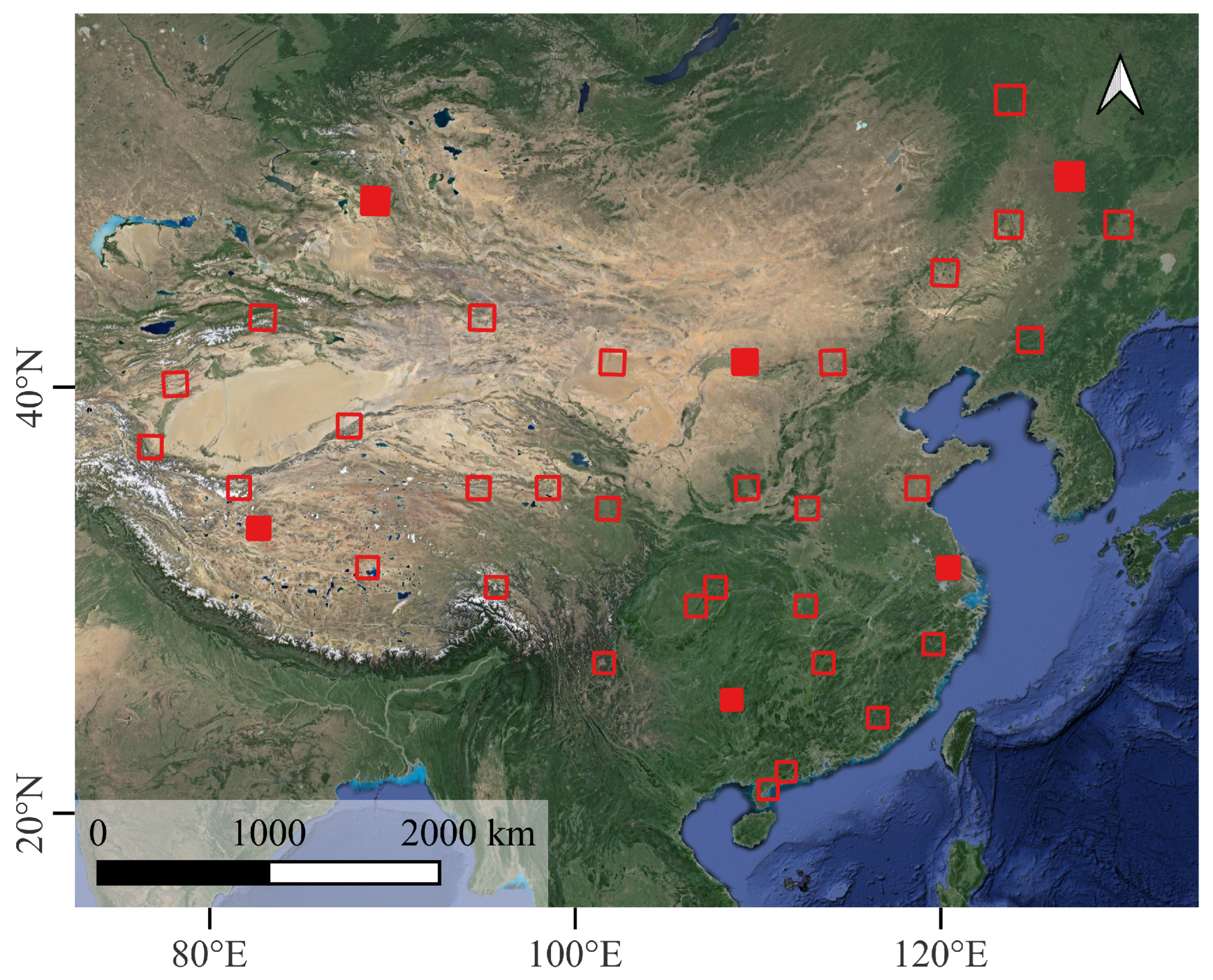
We selected 36 tiles within the domain of mainland China to cover different climate zones and types when constructing the dataset. The spatial distribution of these tiles was the same as that in another Sentinel-2 cloud detection dataset [16], as illustrated in Figure 1. The complete time series of products was collected for each tile. The temporal scope for the majority of the tiles ranged from 2018 to 2019, while for some tiles, it extended from 2016 to 2022. Finally, a total of 13,306 L1C products were collected.
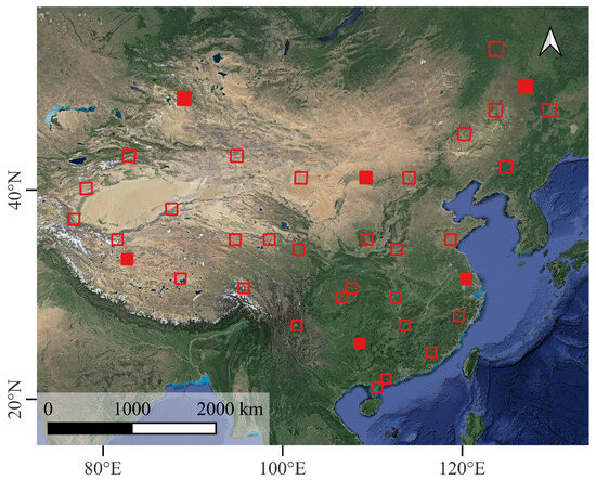
Figure 1.
Distribution of Sentinel-2 Level-1C tiles. The selected 36 tiles are marked with red rectangles, where the filled rectangles are the tiles used for the discussion of the model’s spatial generalization ability in Section 4.6 (Base map: Google Map).
2.2. Class Schema
In the stage of dataset preparation and model runtime, we classified the cloud cover into six categories: clear sky, (opaque) clouds, thin clouds, haze, (cloud) shadow, and ice/snow. The definitions of these categories were primarily derived from the visual appearance of a 60 m × 60 m neighborhood at a specific location, also called the region of interest (ROI), in a time-series TCI rather than their physical characteristics:
- Clear sky was defined as the land surface being clearly observable.
- Opaque clouds were defined as the land surface being totally blocked by clouds.
- Thin clouds were defined as surface features being discernible but located within semi-transparent regions with recognizable shapes.
- Haze was defined as surface features being discernible but located within homogeneous semi-transparent regions (without recognizable shapes).
- Cloud shadows were defined as a sudden decrease being observed in surface reflectance.
- Ice/snow was defined as regions where the surface became white and brighter and exhibited texture or where a melting process was observable.
Thin clouds and haze could sometimes be challenging be to visually distinguish when it was difficult to recognize the shape of the semi-transparent region. Both very slight and heavy semi-transparency effects were defined as haze/thin clouds, which meant that some samples in the haze and thin cloud classes could be similar to those in the clear sky or opaque cloud classes. While this categorization may introduce some imprecision, it was intentionally designed to reduce intra-class differences between clear sky and opaque cloud images. When encountering an ROI containing multiple targets, assign the category of the ROI based on priority. The highest priority is given to “opaque cloud”, followed by “thin cloud”; “cloud shadow”; “haze”; “ice/snow”; and, finally, “clear sky”.
For more details on category interpretation, refer to Section 2.4.
2.3. Overall Framework
Considering the difficulty of making semantic segmentation labels, especially for semi-transparent thin clouds, haze, and cloud shadows [5], we adopted a time-series pixel-wise classification framework based on the composites of the four bands with a 10 m resolution (B2, B3, B4, and B8). In this way, we could reduce the confusion in making labels and ensure consistency between input features and the features from TCIs used for interpretation.
STDL-based cloud detection model architectures take a sequence with image patches, denoted as , as input and yield a sequence of class labels () corresponding to the ROI at each timestamp. Here, t denotes the number of timestamps, denotes the number of bands, and and denote the numbers of rows and columns for each image patch, respectively. The ROI is defined as an area of pixels centered in each composite image, corresponding to an actual area of 60 m × 60 m.
In this setting, a cloud mask with a 60 m resolution could be generated using a sliding-window prediction approach, leading to a significant reduction in computational load compared to that with the original 10 m resolution. However, in practice, models with a short computation time are still required for pixel-wise classification when using deep learning methods. Therefore, in this research, we used shallow and simple models with fewer parameters; for details, see Section 2.5.
2.4. Dataset Construction
First, 500 points were randomly generated for each tile, and all of these points were aligned to the pixel grid center of the bands with a 60 m resolution (e.g., B10) to maintain consistency when comparing them with other products. This was because other cloud detection methods may use the cirrus band, which has a resolution of 60 m, as a feature.
Then, time-series image patches of two different shapes were cropped with each point as the center. Patches with dimensions of were extracted from B2, B3, B4, and B8 to serve as the input TOA reflectance features for the model. Additionally, patches with dimensions of were cropped from the TCI file to serve the purpose of interpreting class labels.
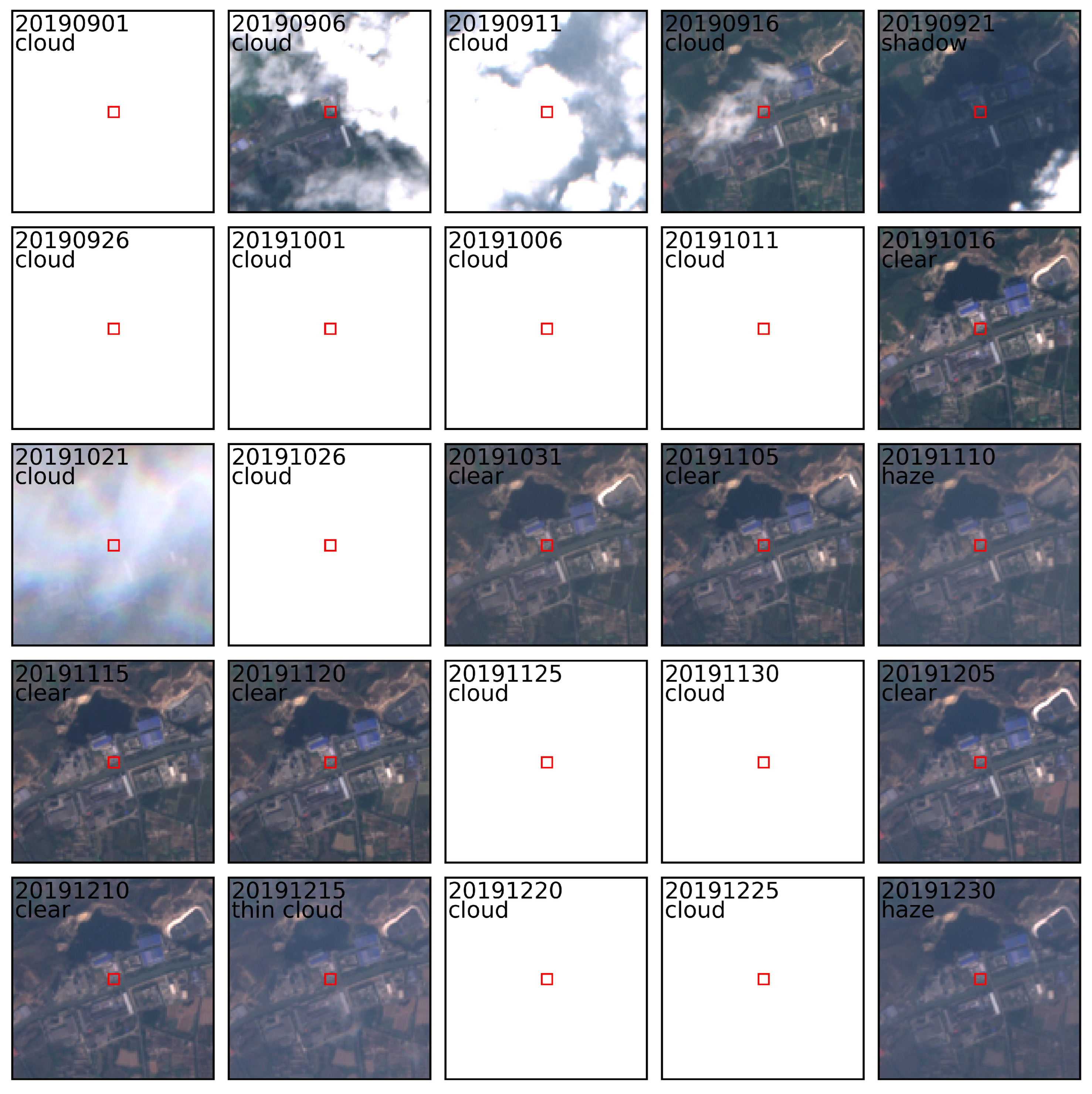
Figure 2 illustrates an example of labeled time-series patches with dimensions of , with the ROI being marked by a red line. All ROIs that intersect with opaque clouds are labeled as thick clouds. When interpreting samples of thin clouds, haze, and shadows, it could help to observe disturbances in brightness or contrast across time-series images. For example, the ROI in the image block dated 10 November 2019 appeared to be slightly brighter and had lower contrast than image blocks from adjacent times, indicating that it may have been obscured by semi-transparent objects. Additionally, it appeared to be homogeneous, with no distinct areas of cloud aggregation, leading to the determination that it was in the haze class. However, for the ROI in the image block dated 15 December 2019, although it also showed disturbances in brightness and contrast, the presence of areas of slight cloud aggregation around (above and below) the ROI led to the determination that it was of the thin cloud class. Other ROIs without an increase in brightness and decrease in contrast compared to adjacent times could be classified as clear sky.
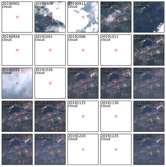
Figure 2.
Example of the interpretation of labels, where the ROI is marked with a red box. The date is labeled in the (year) (month) (day) format.
Despite potential confusion between cloud and snow/ice samples due to brightness saturation, the patches were correctly interpreted as snow/ice if they were subsequently followed by a progression indication of snow/ice melting and were collected during the winter. Additionally, pixels with a normalized difference snow index (NDSI) greater than 0.6 could be considered as ice/snow [10]. We further utilized this index to assist in identifying brightness-saturated ice/snow in the TCIs.
Finally, there were 17,292 groups of labeled time series in total, including 4,450,140 individual image patches and label pairs. The detailed sample numbers for each class are shown in Table 2. This dataset was stored in TFRecord format for better file input performance, and it has been shared at https://zenodo.org/records/10613705 (accessed on 4 February 2024).

Table 2.
Number of samples for each class.
2.5. Spatial–Temporal Deep Learning Models
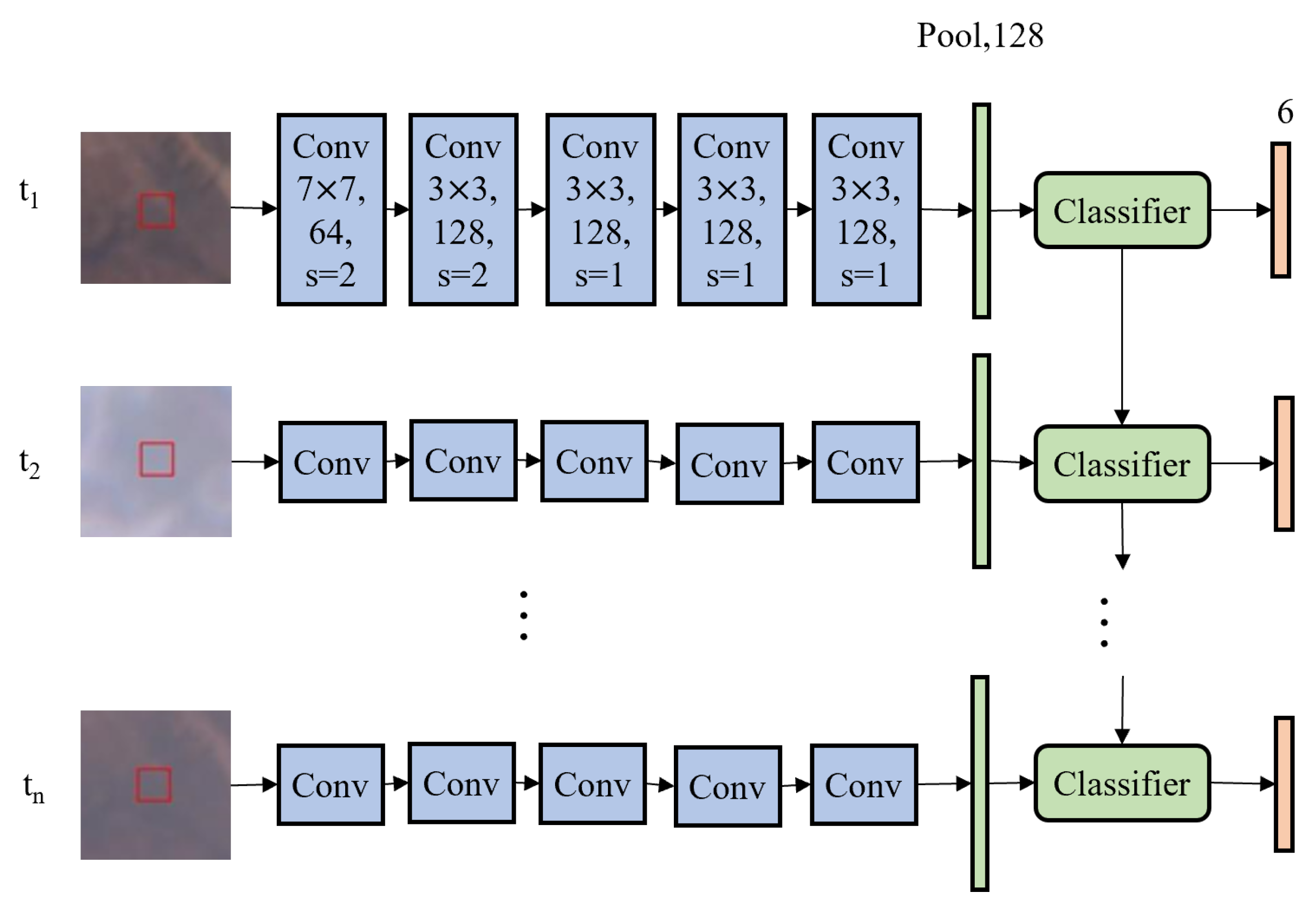
The general architecture of an STDL model is shown in Figure 3. As mentioned in Section 2.3, small and simple models were adopted in this study. In the STDL models, the inputs were first normalized by the means and standard deviations for each band; then, the spatial features of each timestamp were separately extracted by the shared convolutional neural network (CNN) module, followed by global average pooling; finally, the classification module computed the logits of different classes in order, and the prediction labels were generated with the argmax operation. In this study, four STDL models with different classification modules were tested.
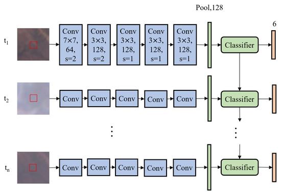
Figure 3.
STDL framework. The red boxes are only the illustrations for ROI, not part of the model inputs.
2.5.1. CNN Module
Considering that the size of input image patches is much smaller than the requirements of state-of-the-art image classification backbones, such as ResNet, EfficientNet [35], etc., a shallow and simple CNN module was used. For the CNN module, the number of filters of each layer was 64, 128, 128, 128, and 128, respectively. The kernel size was for the first layer and for the subsequent four layers. The stride was 2 for the first two layers and 1 for the rest. Each CNN layer was followed by batch normalization and a rectified linear unit (ReLU) activation function. The TimeDistributed layer of Keras was utilized to concurrently apply the shared CNNs. The shape of the CNN output for a time step was , and a spatial feature vector of length 128 was then obtained after global average pooling.
2.5.2. Classification Modules
We tested four types of classification modules: dense, LSTM [36], Bi-LSTM, and transformer [37]. All classifiers took the feature vectors from the CNNs as input and used a dense layer with six units as the output layer to obtain the logits of six classes. The softmax activation function was used in the output layer to obtain the probability distribution across the six classes.
A dense classifier was used as a reference. It had only one dense layer with 128 units as a middle layer, in which the ReLU activation function was used. The dense layer was implemented with the dense layer from the Keras library; it shared the same weights among all time steps and processed them separately by using the TimeDistributed layer of Keras. Thus, it was not able to handle any temporal dependencies.
In the LSTM classifier, an LSTM layer with 128 units was used to encode temporal dependencies. LSTM is a type of RNN in which the output of every time step is affected by both the current and previous inputs. The LSTM layer of Keras was used; the full sequence of outputs was returned to support series classification, and all other parameters were set to their default values.
The Bi-LSTM classifier used a bidirectional LSTM layer with 128 units. This layer separately processed the input sequence backward and forward, and the output sequence was the sum of the two directional outputs. In this way, the output of each time step could be influenced by all inputs. A bidirectional wrapper of Keras was used to implement the bidirectional LSTM.
The transformer architecture has achieved excellent accuracy in recent natural language processing and serial classification applications. In its attention mechanism, each time step can focus on certain parts of the whole sequence and obtain temporal dependencies. Since there was no generation step in our cloud detection task, only the encoder part of the original architecture was used. The transformer encoder is made up of identical encoder blocks. Each block is composed of one self-attention layer and a feedforward network. We used one transformer encoder block containing eight self-attention headers. The feedforward layer in the encoder block had a size of 128 and used the ReLU activation function. We used the same positional encoding method as that in the original transformer: a mixture of sine and cosine functions with geometrically increasing wavelengths [37]. Positional encoding was added to the input of the transformer module to make it aware of positions. The implementation from official TensorFlow models (https://github.com/tensorflow/models/tree/master/official (accessed on 4 February 2024)) was adopted. An overview of the hyperparameters of all of these classifiers can be seen in Table 3. Following common practices from ResNet, we employed a step-wise learning rate schedule, and cross-entropy loss function, and SGD optimizer with a momentum of 0.9 and incorporated a warm-up technique. The model underwent training for 90 epochs with a batch size of 20.

Table 3.
Hyperparameters of the dense, LSTM, Bi-LSTM, and transformer classifiers.
2.5.3. Hyperparameter Optimization
While we explored the hyperparameter space, limitations in computational resources necessitated focusing on a specific range. Because we aimed to obtain a lightweight model suitable for large-scale cloud detection, we started with a larger number of layers, larger layer sizes, and more channels, and we gradually reduced them until there was a significant decrease in the overall accuracy on the validation set.
This step-wise learning rate schedule starts with a base learning rate () that is divided by 10 at specified epochs (30th, 60th, and 80th). After determining the model structure, we explored different base values based on STDL with the LSTM classifier, finally choosing a base of .
2.6. Model Evaluation
For each tile, 80% of the generated sample points were randomly selected as the training set, with the remaining points being reserved for evaluation. The number of validation sample timestamps was as follows: 129,401 for clear sky, 172,500 for (opaque) clouds, 24,431 for thin clouds, 18,458 for haze, 4677 for (cloud) shadows, and 37,533 for ice/snow. The model’s performance was assessed using confusion metrics, precision, recall, and the F1 score.
For clear sky, opaque clouds, and ice/snow, the typical metrics were calculated. However, this was relatively complex for thin clouds, haze, and cloud shadows. Both thin clouds and haze were semi-transparent, had similar effects on images, and had no quantifiable criteria. In addition, thin clouds and haze could cover any type of object, including cloud shadows, which made this more like a multi-label classification task. Thus, some special metrics were further designed in consideration of these characteristics to gain a more comprehensive understanding of the accuracy performance. Practical precision for thin clouds and haze (THPP) is expressed as follows:
Practical recall for thin clouds and haze (THPR) is expressed as follows:
The practical F1 score for thin clouds and haze (THPF1) is expressed as follows:
Practical precision for shadows (SPP) is expressed as follows:
Practical recall for shadows (SPR) is expressed as follows:
The practical F1 score for shadows (SPF1) is expressed as follows:
where denotes the value in the row of the true label (i) and the column of the predicted label (j) from the confusion matrix (). The short names of these classes are C for clear sky, O for opaque clouds, T for thin clouds, H for haze, S for cloud shadows, and I for ice. In the definitions of THPP, THPR, and THPF1, the errors from opaque clouds and cloud shadows were ignored because (1) masking heavy thin clouds and haze as opaque is acceptable when avoiding interference, (2) thin clouds and haze are sometimes so similar that there may be potential ambiguities in their differentiation, (3) some thin clouds and haze are usually mixed with cloud shadows near opaque clouds, and (4) there could be further processing in downstream applications to remove this semi-transparency and enhance the ground information [38]. Similarly, we defined SPP, SPR, and SPF1, in which the errors from thin clouds and haze for cloud shadows were also ignored.
Furthermore, some metrics were specifically defined to assess the effectiveness of masking “poor” or “good” data in various situations and to adapt to different classification schemes. These metrics were groups of precision, recall, and F1 score. The positive class of each group was the union of fine classes for a specified purpose. The details of the positive classes and abbreviations for each metric group are listed in Table 4.

Table 4.
Definitions and abbreviations for different metrics.
The semi-transparency data mask regarded thin clouds and haze as positive classes. The general invalid data mask regarded opaque clouds, thin clouds, haze, and cloud shadows as positive classes, while the stricter one ignored haze. The general usable data mask regarded clear sky, ice/snow, and haze as positive classes. The general cloud mask regarded opaque clouds, thin clouds, and haze as positive classes. The general non-cloud mask regarded clear sky, haze, cloud shadows, and ice/snow as positive classes. All of these stricter metrics excluded the haze class.
2.7. Comparison of Methods
Due to the absence of a large-scale annotated time-series cloud detection dataset before this study, it was difficult to find supervised machine learning methods for time-series cloud detection to use for comparison. We compared the results of our method with those of the s2cloudless [22], MAJA (MACCS-ATCOR Joint Algorithm, where MACCS is Multi-Temporal Atmospheric Correction and Cloud Screening, and ATCOR is Atmospheric Correction) [10], and Cloud Score+ [34] methods. The s2cloudless method, an official algorithm designed for generating cloud masks with a resolution of 60 m, utilizes 10-band reflectance data from a single-period image and is based on a gradient-boosting algorithm. It is considered the state of the art and was identified on the Pareto front among 10 cloud detection algorithms by Skakun et al. [5]. The MAJA algorithm is a multi-temporal approach that generates cloud masks at a resolution of 240 m. The results obtained from MAJA served as training samples during the development of the s2cloudless algorithm. Cloud Score+, which was proposed by Google LLC, Mountain View, CA, USA, has been available on the Google Earth Engine since the end of 2023. It utilizes a weakly supervised deep learning methodology to assess the quality of individual image pixels in comparison with relatively clear reference images. We exported the official Cloud Score+ time-series values of the validation points at a resolution of 60 m from the Google Earth Engine for comparison.
This comparison may have been biased due to the different classification schemas used by the algorithms. The s2cloudless method only identified non-clouds and clouds. The MAJA algorithm was able to detect clouds, thin clouds, cloud shadows, and high clouds separately, and a single pixel could have multiple classification labels. In particular, the Cloud Score+ method ignored the definition of different classes and gave a quality score that indicated the degree to which a pixel was like a clear pixel.
To maintain consistency in the comparison, we remapped these classes and used the metrics for usable masks and all cloud masks shown in Table 4. Due to the slow processing speed of MAJA, only a subset of the products was selected for comparison.
3. Results
3.1. Comparison of the STDL Metrics
Table 5 presents the values of the various evaluation metric groups (see Table 4) for the four STDL models, and the highest F1 score values are highlighted in bold and underlined.

Table 5.
Evaluation metrics for the STDL models. The highest F1 score values among different model are highlighted in bold and underlined.
3.1.1. Perspectives of the Models
Generally, the STDL models equipped with the dense and normal LSTM classifiers demonstrated inferior performance with respect to those utilizing the Bi-LSTM and transformer classifiers. All of the metric groups indicated marginal differences between Bi-LSTM and the transformer.
The dense classifier was the worst, and there was a large gap between it and the other models in terms of both standard/practical semi-transparency and cloud shadows. However, for the other metric groups of clear sky, opaque clouds, cloud/non-cloud masks, and usable/invalid masks, the F1 scores had high values above 0.9. With regard to the LSTM classifier, the F1 scores increased by approximately 0.04 and 0.11 for semi-transparency and cloud shadows, respectively.
The Bi-LSTM classifier showed slightly higher F1 scores than those of the transformer for most metric groups, except for clear sky, opaque clouds, and cloud shadows.
3.1.2. Perspectives of the Metric Groups
Generally, across the eight coarse mask metric groups (general/stricter “invalid”, “usable”, “cloud”, and “non-cloud” masks), the F1 scores consistently demonstrated high values, with minimal variation among the different models and the maximum difference being less than 0.02. The general invalid mask achieved the highest F1 score of 0.9567 when using the Bi-LSTM classifier.
In terms of fine categories, “opaque clouds” consistently exhibited the highest F1 scores, reaching 0.9653 with the transformer classifier. Similarly, “clear sky” also attained relatively higher F1 scores, with the transformer model achieving the highest values.
Conversely, both “cloud shadows” and “semi-transparency” consistently yielded the lowest F1 scores, although the practical metrics notably outperformed them. For the “ice/snow” category, the metrics fell within a moderate range, with the highest F1 score being recorded as 0.89 with Bi-LSTM.
3.1.3. Results of the Confusion Metrics
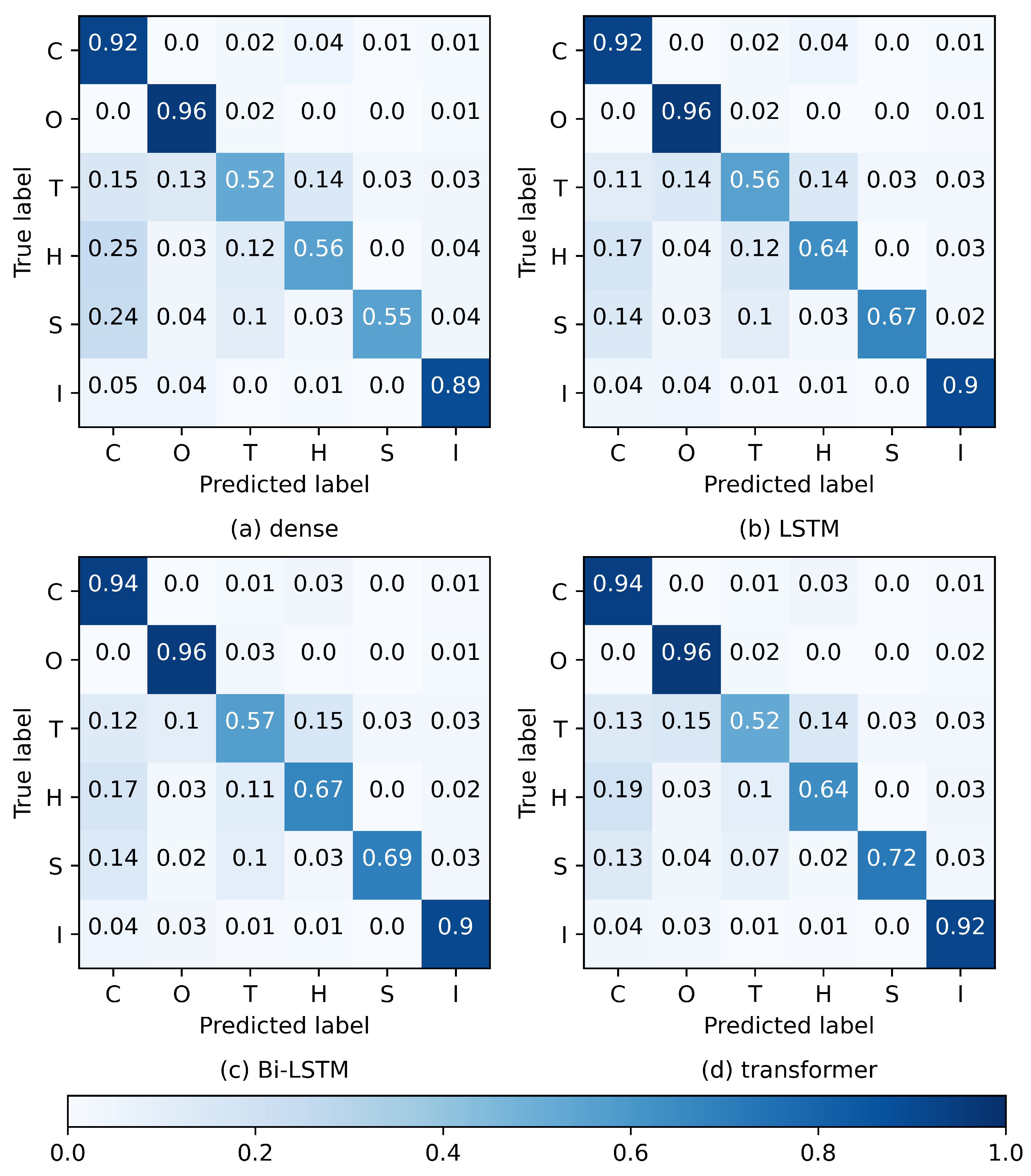
The confusion matrix presented in Figure 4 further highlighted specific instances of classification errors; decimals indicate the fraction of corresponding ground-truth labels. Overall, these four models demonstrated relatively consistent patterns in classifying incorrectly.
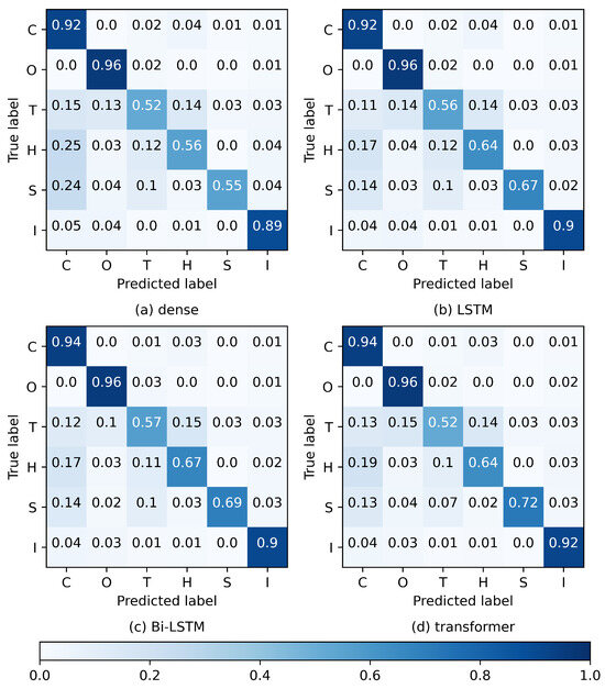
Figure 4.
Confusion metrics on the evaluation dataset for the four STDL models with the (a) dense, (b) LSTM, (c) Bi-LSTM, and (d) transformer classifiers. Decimals indicate the fraction of corresponding ground-truth labels. Mapping of class names: C for clear sky, O for opaque clouds, T for thin clouds, H for haze, S for cloud shadows, and I for ice.
- There were almost no errors between opaque clouds and clear skies. Classification errors for clear skies predominantly occurred with haze, with minimal instances involving thin clouds and ice/snow.
- Opaque clouds were primarily incorrectly classified as thin clouds, with fewer instances being classified as ice/snow.
- The classification errors for thin clouds encompassed clear skies, opaque clouds, and haze, with a small number of cases involving cloud shadows and ice/snow.
- The haze classification errors were predominantly observed with clear skies, with few occurrences with thin clouds, opaque clouds, and ice/snow.
- The cloud shadow classification errors primarily involved clear skies and thin clouds, with a small number occurring in opaque clouds, haze, and ice/snow.
- The classification errors for ice/snow mainly involved clear skies and opaque clouds, with a few instances in thin clouds and haze and essentially no errors with cloud shadows.
3.2. Computational Cost
Table 6 lists the parameter count, model training time (based on the training dataset and running for 90 epochs), and inference time on the validation dataset for the four models. Overall, among the four models discussed in this study, except for the model based on the dense classifier, the model using the transformer classifier had the lowest parameter count, as well as the shortest training and inference times, while the Bi-LSTM model has the largest number of parameters and the longest computing time.

Table 6.
Number of model parameters, training time on the training dataset, and inference time for the validation dataset.
3.3. Spatial Variance
In this section, we further explore the performance variations of the STDL models across different regions. Given the minimal differences in accuracy performance among these STDL models and the proximity in the distribution of classification errors, we chose the model with the transformer classifier as representative, as it had fewer parameters and a shorter runtime. To avoid redundancy and considering the downstream task’s practical need for the removal of “poor” data, we illustrated the spatial variations using F1 scores for the general usable mask and stricter usable mask as representatives. The spatial distributions of these two metrics are illustrated in Figure 5.
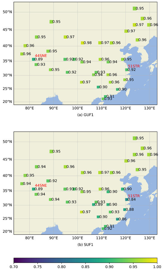
Figure 5.
The spatial variance in F1 scores for the general usable mask (a) and stricter usable mask (b). The base map depicts the distribution of land and ocean. The names of two special tiles discussed in the main text are marked in red above the metric values.
Figure 5a displays the spatial distribution of F1 score for the general usable mask, where the majority of tiles exhibited a high F1 score (close to or above 0.95), but the tile named ‘44SNE’ had the lowest value of 0.89; see the red annotation in the figure. This tile was situated in the western Qinghai–Tibet Plateau region.
Figure 5b depicts the spatial distribution of F1 score for the stricter usable mask, where, for the majority of the tiles, the values closely aligned with those of the F1 score for the general usable mask. However, in some tiles located in the southeastern part, the F1 score for the stricter usable mask significantly decreased, with the most significant decrease being 0.08, which was observed in tile 51STR, reaching a value of 0.84.
The detailed cloud detection figures of the STDL models in different regions are jointly presented with other existing products in Section 3.4.2.
3.4. Comparison with Other Algorithms
3.4.1. Comparison of Metrics
Table 7 presents the values of the usability mask metrics and all-cloud mask metrics for the s2cloudless, MAJA, CS+, and STDL models. Different official recommended thresholds were applied to binarize the two scores (cs and cs_cdf) in the CS+ products, and the metrics were calculated accordingly. The numbers following the dashes in the table header indicate the thresholds used for binarization. The STDL models using the Bi-LSTM and transformer classifiers were chosen as representatives for this comparison.

Table 7.
Comparison of metrics for the s2cloudless, MAJA, CS+, and STDL models. The words ‘cs’ and ‘cs_cdf’ are the two scores of the CS+ method. The numbers following the hyphens in the table header indicate the thresholds used for binarization.
In summary, all metric scores of the STDL models outperformed those of the other three methods, showcasing their overall superior performance.
The s2cloudless method exhibited moderate cloud detection capabilities. The F1 score for the general usable mask was only higher than MAJA; the F1 score for the stricter usable mask was higher than that in MAJA, cs_cdf-0.5, and cs_cdf-0.65; the F1 score for the general cloud mask was higher than that in MAJA, cs-0.5, cs_cdf-0.5, and cs_cdf-0.65; and the F1 score for the stricter cloud mask was higher than that in MAJA and cs_cdf-0.5. The precision values of the usable data and general clouds were lower than the recall values, while the recall of strict clouds was higher than the precision.
MAJA always achieved the lowest F1 scores among these methods. However, the precision for the general usable mask was still higher than that of s2cloudless, cs-0.5, cs_cdf-0.5, cs_cdf-0.65, STDL (Bi-LSTM), and STDL (transformer), and the precision for the stricter usable mask was also higher than that of s2cloudless, cs-0.5, cs_cdf-0.5, and cs_cdf-0.65.
For the CS+ method, the different binarization thresholds showed different tendencies for precision against recall. Compared to cs, cs_cdf had a lower recall for clouds, which was consistent with the descriptions in the official documentation, showing that cs_cdf was less sensitive to thin clouds than cs was. Among the four CS+ score thresholds, cs-0.5 had the highest F1 scores for the general usable mask and stricter cloud mask, while cs-0.65 had the highest F1 scores for the stricter usable mask and general cloud mask.
3.4.2. Visual Comparison
This section showcases the performance disparities among the four methods (STDL, s2cloudless, MAJA, and CS+) across various geographical regions, emphasizing their capabilities in handling distinct cloud characteristics. The TCIs are also plotted for reference.
For visual consistency, category mapping was applied to s2cloudless and MAJA. In s2cloudless, cloud mapping corresponded to the category of opaque clouds. For the results of MAJA, each pixel contained multiple labels, and the priority for selecting the drawing type was as follows (from high to low): cloud shadows, thin clouds, and clouds, with the cloud mapping corresponding to opaque clouds. Additionally, pixels only marked as the ‘high cloud’ type in the results of MAJA were retained and are presented separately. This was due to the fact that ‘high clouds’ were detected in the cirrus band and could be extremely thin or thick, making them difficult to merge into other categories.
For the CS+ products, to maximize the display of details in non-clear-sky data, we chose the cs score, which had a high cloud recall value. We linearly stretched the values within the range from 0 to 0.65. Values exceeding 0.65 are displayed in white.
Figure 6 displays the cloud detection results for four TCI patches. Each column corresponds to a TCI patch, and each row corresponds to a method. The actual extent of all tiles was 30 km × 30 km. The tile name, date, and center coordinates (in decimal latitude and longitude) for the TCI patches were as follows:
- (a)
- 47TQF, 3 April 2019, (41.316, 102.374);
- (b)
- 49TCF, 4 October 2019, (40.963, 109.614);
- (c)
- 51TWM, 7 April 2019, (46.498, 123.525);
- (d)
- 51STR, 16 October 2019, (31.808, 120.121).
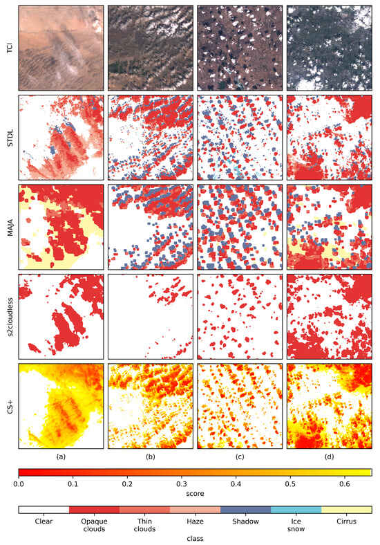
Figure 6.
Cloud detection results of STDL (second row), MAJA (third row), s2cloudless (fourth row), and CS+ (fifth row) for the TCI patches of four sites in the first row. Details of location and date for the sites in columns (a), (b), (c) and (d) can be found in the description in the main text.
Figure 6.
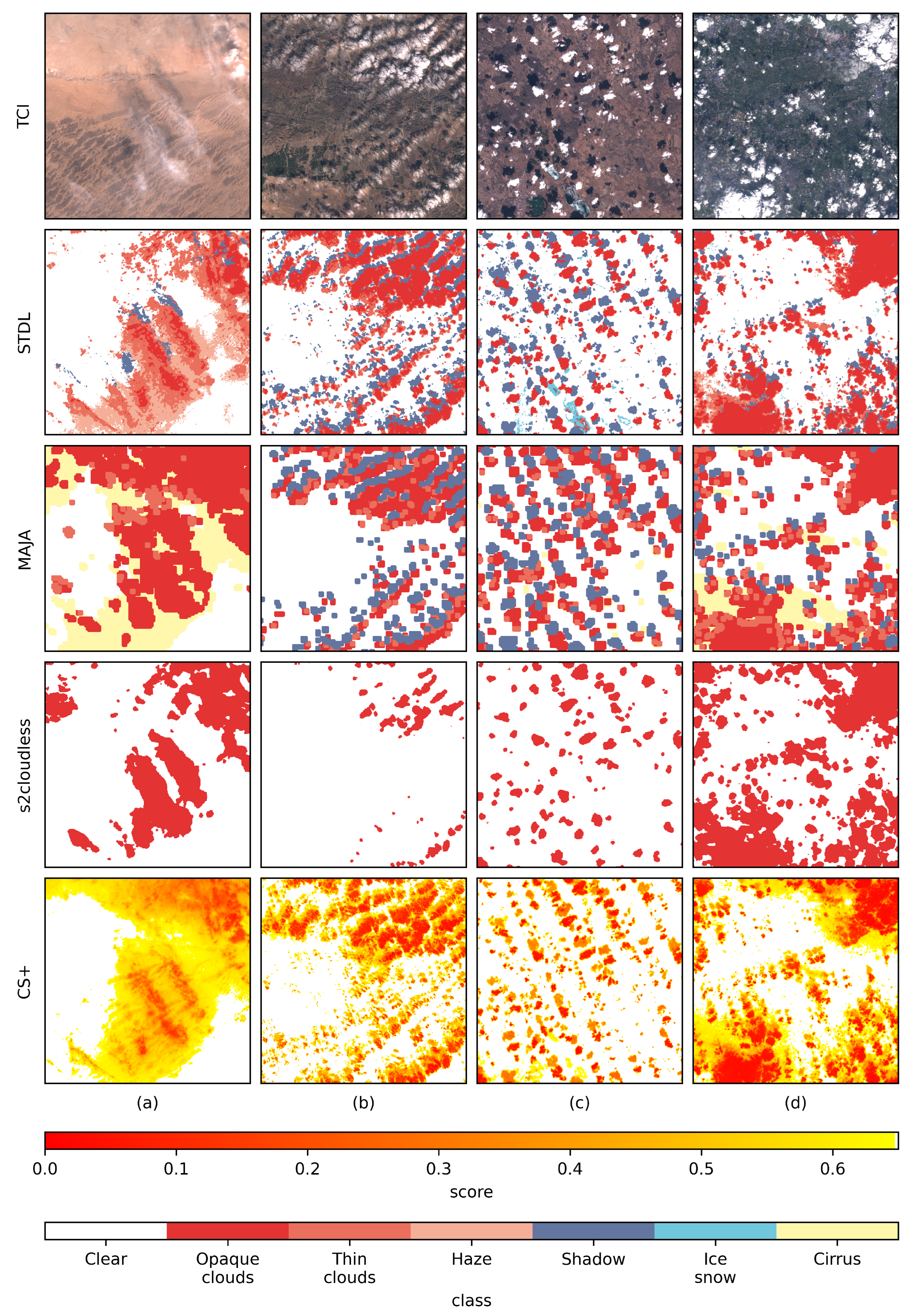
Cloud detection results of STDL (second row), MAJA (third row), s2cloudless (fourth row), and CS+ (fifth row) for the TCI patches of four sites in the first row. Details of location and date for the sites in columns (a), (b), (c) and (d) can be found in the description in the main text.
In this figure, the STDL model extracted the distributions of opaque clouds, thin clouds, haze, and cloud shadows with fine details for all four tiles. Overall, the MAJA algorithm exhibited relatively few omissions and could detect various types of clouds and shadows. However, it showed some false alarms, as seen in the upper part of (a), and it missed some extremely small clouds and shadows, as observed in (b), with a relatively coarse spatial resolution. Additionally, some cirrus clouds in MAJA were not observed in the TCIs—for example, in (d). Some smaller clouds were falsely detected as cirrus clouds, as seen in (c). The s2cloudless algorithm could not provide any information about cloud shadows and missed some thinner or smaller low-level clouds—for instance, in the upper left of (b) and (c). Some thinner clouds or haze were labeled as clouds, as is evident in the upper left of (a) and lower left of (d). For the CS+ method, it could be observed that the chosen threshold identified almost all non-clear-sky areas, but it missed a small amount of shadow from thin clouds (e.g., in the lower left of (a)), and there were some commissions in clear-sky areas (e.g., (d), right side).
4. Discussion
4.1. Motivation
Our motivation for undertaking this work was to enhance cloud detection accuracy when using Sentinel-2 data, especially for cloud shadows and thin clouds, with the aim of ensuring that downstream remote sensing applications can minimize interference from clouds while avoiding excessive loss of usable data.
In our comparative experiments, we observed that the s2cloudless method, which is the state of the art and was provided by official Sentinel-2 sources, failed to offer any information for removing cloud shadows and, at the same time, missed some thin and low-altitude clouds.
Improving capabilities for the detection of thin clouds and shadows is particularly challenging, as their boundaries are difficult to quantify, and most existing datasets do not include information on thin clouds and shadows. Using time-series data can make thin clouds and shadows more distinguishable.
However, it is challenging to find datasets that are suitable for training and validating supervised deep learning models on time-series data. To address this, we also constructed a more detailed time-series cloud detection dataset.
4.2. Classification System
Defining various cloud types and cloud shadows based only on image features is difficult. When designing the classification system for the dataset and STDL models, we did not attempt to address the definitions related to clouds, thin clouds, etc.
From the perspective of utilizing deep learning models, our approach was to reduce intra-class variance, leading us to roughly design a classification system comprising six categories based on the visual characteristics of TCIs. In addition, we employed a time-series interpretation approach based on TCIs to enhance the visual distinctions among different cloud types and shadows.
In the results, it is evident that the six-category classification strategy was effective. As shown in Table 5, opaque clouds, clear sky, and usable data exhibited very high classification accuracy. Additionally, the confusion matrices in Figure 4 indicate that opaque clouds were almost never misclassified as clear sky or haze, and clear sky was almost never misclassified as clouds. This characteristic is useful in practice, as the cloud detection step is typically expected to remove invalid data.
4.3. Input Feature Space
In this study, we primarily enhanced cloud detection accuracy through spatial and temporal features while utilizing only four spectral bands, namely blue, green, red, and near-infrared. This decision was based on the following reasons:
- The model read the entirety of the time-series data at once during inference. Using more bands would increase the runtime, data loading workload, and memory usage, which would not be conducive to applying the model to inference on massive datasets. In addition, through our testing, we did not observe an improvement in accuracy by directly increasing the number of input channels based on the current model structure.
- The different categories were defined based only on the visual features in TCIs. Introducing more bands may require the redefinition of categories. For example, some very thin, high-altitude cirrus clouds that were almost invisible in the TCIs were classified as clear sky, but they could be detected using cirrus bands.
According to Table 5 and Figure 4, even the STDL–dense model, which utilized only spatial features, demonstrated high accuracy in classifying opaque clouds and usable data. Additionally, the confusion matrix showed almost no misclassification of opaque clouds and clear skies. After introducing time-series information, the accuracy of the extraction of thin clouds and shadows significantly improved—in particular, the omission errors were significantly reduced. This confirmed the effectiveness of incorporating temporal and spatial features when enhancing cloud detection.
4.4. Limitations
4.4.1. Ice/Snow
The interpretation based on TCIs made it more challenging to distinguish between opaque clouds and snow/ice, as they both appeared to be saturated in the TCIs. Consequently, some confusion between opaque clouds and snow/ice was inevitable in this dataset. Although using shortwave infrared bands could help in the identification of snow/ice, it would further complicate the construction of the time-series dataset. Hence, they were not employed during the construction of the dataset.
The accuracy evaluation results also confirmed this issue: The confusion matrices in Figure 4 report approximately 3% of snow/ice being misclassified as clouds. The tile labeled ‘44SNE’ in Figure 5 also exhibited lower accuracy in usable data. This tile was located in the Qinghai–Tibet Plateau region, which contains some glaciers and has a significant presence of snow/ice in winter; at the same time, it is often influenced by clouds.
4.4.2. Haze
We defined the category of ‘haze’ from the perspective of image features, but it may actually encompass various types of aerosols. Due to differences in the color rendering of different screens during interpretation, confused labels are inevitable, especially for image patches that are less affected by aerosols. In regions that are frequently influenced by aerosols, the lack of sufficient clear-sky image patches for reference increases the confusion. The spatial variations in the accuracy distribution shown in Figure 5 also confirmed this issue. The difference between the F1 score for the general usable mask and the F1 score for the stricter usable mask was more significant in the relatively humid southeast region. Despite this, users can still flexibly choose the opaque cloud, thin cloud, and cloud shadow categories based on their needs to mask the data and avoid the interference of haze-type errors in local areas.
4.4.3. Single Labels
Unlike typical land cover classifications, the categories in this study were not entirely mutually exclusive. For example, an ROI can simultaneously contain thin clouds, cloud shadows, and snow. However, due to the significant workload involved in annotating time-series data, we only created a single-label dataset.
This may not fully capture the complexity of cloud and cloud shadow coverage, and the label annotations may be influenced by the annotators’ biases. Exploring methods for rapidly constructing multi-label datasets in the future, along with the utilization of appropriate loss functions, holds promise for further enhancing model accuracy and practical utility.
4.4.4. Features
The use of more bands can enrich the features of targets. However, as mentioned in Section 4.3, the model structure used in this study may not have effectively leveraged the information from additional bands.
The reasons could be the increasing feature complexity. From experience in manual interpretation, for example, some thin clouds, haze, and clear skies may be challenging to distinguish in the shortwave infrared band, and some low-altitude opaque clouds are not apparent in the cirrus band.
Perhaps employing a more flexible structure, such as multi-scale branch inputs or channel attention, could allow for the better utilization of a larger feature space. We have not explored this avenue to date due to the trade-off between the costs and potential accuracy gains.
4.5. Model Comparison
The STDL model using Bi-LSTM as a classifier had the highest overall accuracy, but the model’s inference time was longer. On the other hand, the STDL model based on the transformer classifier performed similarly overall but had a faster inference speed.
For the goal of cloud detection, a higher recall is more practically valuable than precision. The s2cloudless method achieved a higher recall for the stricter cloud mask than those of MAJA and certain SC+ thresholds, indicating that it is an excellent method.
However, the goal of detecting usable data is more practically meaningful than detecting clouds. Although the MAJA method exhibited lower accuracy in cloud detection, it had a better ability to detect usable data. In particular, the precision values for the general usable mask and stricter usable mask of MAJA were significantly higher than those of s2cloudless and certain SC+ thresholds, indicating that the usable data labels provided by the MAJA method were highly reliable. Of course, this came at the cost of sacrificing recall, leading to the omission of some usable data.
In the process of preparing this study, we noticed that the Google team had introduced the CS+ algorithm, and we included it in the method comparisons in this study. The CS+ algorithm requires users to explore score thresholds for different data to balance the precision and recall. Increasing the CS+ score threshold decreases the recall of usable data and increases the precision. For the dataset used in this study, cs-0.5 had the highest F1 score for the general usable mask, and cs-0.65 had the highest F1 score for the stricter usable mask, both of which were lower than those of the simple supervised STDL models used here. Although this method can provide high-quality binary masks for usable data, it cannot distinguish thin clouds, haze, and cloud shadows for various post-processing applications, such as image enhancement in areas with thin clouds and shadows.
4.6. Spatial Generalization Ability
Using as many representative datasets as possible to train the model is crucial for engineering applications. Therefore, the training data used in our previous experiments came from all 36 tiles. In Figure 5, it can be observed that the F1 scores are relatively lower at certain locations, such as the tiles near the coastal land. We investigated and found that the direct reason is that the proportion of ROIs of thin clouds and haze is relatively larger compared to other regions, and their accuracies are relatively lower than those of opaque clouds and clear sky, thus lowering the average F1 scores.
In this section, to further discuss the model’s spatial generalization ability, we split the training and testing sets based on tiles, then conducted training and evaluation.
The tiles used for testing need to encompass a variety of terrains and landforms to ensure the reliability of the evaluation results. Because we had a relatively small number of tiles, we manually selected six of them for validation rather than randomly selecting tiles for cross-validation. The positions of these six validation tiles are marked with filled rectangles in Figure 1.
Then, we trained the STDL model using training points from the other 30 tiles in the dataset and evaluated the model using validation points from these 6 validation tiles. Similar to Section 3.3, only the STDL models using the transformer classifier were tested. For convenience, this trained model is named ‘STDL-val’ in the following.
The F1 scores for the general/stricter usable and cloud masks were used for comparison. We also recalculated the F1 scores for other methods (s2cloudless, MAJA, and CS+) using validation points from these validation tiles. The F1 scores of different mask types for different methods are listed in Table 8.

Table 8.
The F1 scores of different mask types for different methods, which were calculated using the validation points from the 6 validation tiles. Only the STDL models using the transformer classifier are compared here. The word ‘STDL-val’ represents the STDL model trained using only sample points from the 30 non-validation tiles.
Compared to the original trained STDL model, the STDL-val model’s F1 scores for all four masks experienced a slight decrease. This could be attributed to a reduction in correlation between training and testing data—typically, points spatially closer in space exhibited greater correlation [39]. Additionally, reducing the amount of training data may lead to a poorer model. Nonetheless, the F1 scores of the STDL-val model still surpass those of other existing methods. This result indicates that extending the STDL model constructed in this study for cloud detection in Sentinel-2 data to other regions in China is promising.
5. Conclusions
In this study, we explored the effectiveness of using a simple supervised spatial–temporal deep learning model for fine-grained cloud detection in time-series Sentinel-2 data. Simultaneously, we contributed the first long-time-series dataset specifically designed for cloud detection to facilitate both model development and accuracy assessment. To avoid boundary uncertainty, we designed the models and constructed the dataset based on a pixel-wise classification framework.
Drawing inspiration from existing research on deep learning models for time-series classification, we built four simple sequence-to-sequence classification models. All of these models took four bands with a resolution of 10 m as input, utilized multi-layer CNNs with shared weights as spatial feature extractors, and employed a fully connected dense layer, LSTM, Bi-LSTM, and transformer as classifiers.
The results showed that the supervised STDL models could produce a detailed cloud mask with thin clouds and cloud shadow information, while most cloud detection methods only produced a binary mask. The STDL models with the Bi-LSTM classifier and transformer classifier exhibited close performance and were better than the other two classifiers. Although the model accuracy of the transformer classifier was slightly lower than that of Bi-LSTM, it had higher computational efficiency. This cost-effectiveness enables the generation of high-quality usable data masks for large data volumes.
In this study, we only used the visual effects of TCIs to define categories, we designed datasets and models based solely on single-label classification tasks, and we used only four 10 m bands, which may have hindered the learning of complex cloud and cloud shadow coverage patterns. In addition, the time interval between the overlap areas of adjacent satellite scanning paths was half the normal revisit period. We temporarily ignored the potential effects of the time interval on model accuracy in this study.
Future research endeavors include extending the STDL models to more satellite imagery, such as that of the Chinese Gaofen series, as well as to multi-label classification tasks, and handling more spectral bands. In addition, building a deep learning model for computationally efficient single-period segmentation while leveraging the accurate cloud masks generated by an STDL model presents an intriguing avenue for further exploration.
Author Contributions
Conceptualization, R.Y. and C.G.; methodology, C.G.; software, R.Y.; validation, C.G., R.Y. and T.L.; formal analysis, C.G. and R.Y.; resources, G.H.; data curation, R.Y.; writing—original draft preparation, C.G.; writing—review and editing, T.L.; visualization, R.Y.; supervision, W.J.; project administration, G.H.; funding acquisition, G.W. All authors have read and agreed to the published version of the manuscript.
Funding
This research was funded by the Fund for Pioneering Research in Science and Disruptive Technologies through the Aerospace Information Research Institute at the Chinese Academy of Sciences (Grant No. E3Z218010F).
Data Availability Statement
The dataset is shared at https://zenodo.org/records/10613705 (accessed on 4 February 2024).
Conflicts of Interest
The authors declare no conflicts of interest. The funders had no role in the design of the study; in the collection, analyses, or interpretation of data; in the writing of the manuscript; or in the decision to publish the results.
Abbreviations
The following abbreviations are used in this manuscript:
| ReLU | Rectified Linear Unit |
| LSTM | Long Short-Term Memory |
| Bi-LSTM | Bidirectional Long Short-Term Memory |
| CNN | Convolutional Neural Network |
| TCI | True-Color Image |
| ROI | Region of Interest |
| STDL | Spatial–Temporal Deep Learning |
| CM | Confusion Metric |
| TOA | Top-of-Atmosphere |
| MAJA | MACCS-ATCOR Joint Algorithm |
| MACCS | Multi-Temporal Atmospheric Correction and Cloud Screening |
| ATCOR | Atmospheric Correction |
References
- Lv, Z.; Liu, T.; Benediktsson, J.A.; Falco, N. Land Cover Change Detection Techniques: Very-high-resolution Optical Images: A Review. IEEE Geosci. Remote Sens. Mag. 2022, 10, 44–63. [Google Scholar] [CrossRef]
- Yin, R.; He, G.; Wang, G.; Long, T.; Li, H.; Zhou, D.; Gong, C. Automatic Framework of Mapping Impervious Surface Growth With Long-Term Landsat Imagery Based on Temporal Deep Learning Model. IEEE Geosci. Remote Sens. Lett. 2022, 19, 2502605. [Google Scholar] [CrossRef]
- You, Y.; Wang, S.; Pan, N.; Ma, Y.; Liu, W. Growth Stage-Dependent Responses of Carbon Fixation Process of Alpine Grasslands to Climate Change over the Tibetan Plateau, China. Agric. For. Meteorol. 2020, 291, 108085. [Google Scholar] [CrossRef]
- Amani, M.; Ghorbanian, A.; Ahmadi, S.A.; Kakooei, M.; Moghimi, A.; Mirmazloumi, S.M.; Moghaddam, S.H.A.; Mahdavi, S.; Ghahremanloo, M.; Parsian, S.; et al. Google Earth Engine Cloud Computing Platform for Remote Sensing Big Data Applications: A Comprehensive Review. IEEE J. Sel. Top. Appl. Earth Obs. Remote Sens. 2020, 13, 5326–5350. [Google Scholar] [CrossRef]
- Skakun, S.; Wevers, J.; Brockmann, C.; Doxani, G.; Aleksandrov, M.; Batič, M.; Frantz, D.; Gascon, F.; Gómez-Chova, L.; Hagolle, O.; et al. Cloud Mask Intercomparison eXercise (CMIX): An Evaluation of Cloud Masking Algorithms for Landsat 8 and Sentinel-2. Remote Sens. Environ. 2022, 274, 112990. [Google Scholar] [CrossRef]
- Main-Knorn, M.; Pflug, B.; Louis, J.; Debaecker, V.; Müller-Wilm, U.; Gascon, F. Sen2Cor for Sentinel-2. In Image and Signal Processing for Remote Sensing XXIII; Bruzzone, L., Bovolo, F., Benediktsson, J.A., Eds.; SPIE: Warsaw, Poland, 2017; p. 3. [Google Scholar] [CrossRef]
- Qiu, S.; Zhu, Z.; He, B. Fmask 4.0: Improved Cloud and Cloud Shadow Detection in Landsats 4–8 and Sentinel-2 Imagery. Remote Sens. Environ. 2019, 231, 111205. [Google Scholar] [CrossRef]
- Zhang, H.; Huang, Q.; Zhai, H.; Zhang, L. Multi-Temporal Cloud Detection Based on Robust PCA for Optical Remote Sensing Imagery. Comput. Electron. Agric. 2021, 188, 106342. [Google Scholar] [CrossRef]
- Hagolle, O.; Huc, M.; Pascual, D.V.; Dedieu, G. A Multi-Temporal Method for Cloud Detection, Applied to FORMOSAT-2, VENμS, LANDSAT and SENTINEL-2 Images. Remote Sens. Environ. 2010, 114, 1747–1755. [Google Scholar] [CrossRef]
- Hagolle, O.; Huc, M.; Desjardins, C.; Auer, S.; Richter, R. MAJA Algorithm Theoretical Basis Document; Zenodo: Geneva, Switzerland, 2017. [Google Scholar] [CrossRef]
- Zhu, Z.; Woodcock, C.E. Automated Cloud, Cloud Shadow, and Snow Detection in Multitemporal Landsat Data: An Algorithm Designed Specifically for Monitoring Land Cover Change. Remote Sens. Environ. 2014, 152, 217–234. [Google Scholar] [CrossRef]
- Qiu, S.; Zhu, Z.; Woodcock, C.E. Cirrus Clouds That Adversely Affect Landsat 8 Images: What Are They and How to Detect Them? Remote Sens. Environ. 2020, 246, 111884. [Google Scholar] [CrossRef]
- Zhu, X.; Helmer, E.H. An Automatic Method for Screening Clouds and Cloud Shadows in Optical Satellite Image Time Series in Cloudy Regions. Remote Sens. Environ. 2018, 214, 135–153. [Google Scholar] [CrossRef]
- Goodwin, N.R.; Collett, L.J.; Denham, R.J.; Flood, N.; Tindall, D. Cloud and Cloud Shadow Screening across Queensland, Australia: An Automated Method for Landsat TM/ETM+ Time Series. Remote Sens. Environ. 2013, 134, 50–65. [Google Scholar] [CrossRef]
- Li, Z.; Shen, H.; Weng, Q.; Zhang, Y.; Dou, P.; Zhang, L. Cloud and Cloud Shadow Detection for Optical Satellite Imagery: Features, Algorithms, Validation, and Prospects. ISPRS J. Photogramm. Remote Sens. 2022, 188, 89–108. [Google Scholar] [CrossRef]
- Li, J.; Wu, Z.; Hu, Z.; Jian, C.; Luo, S.; Mou, L.; Zhu, X.X.; Molinier, M. A Lightweight Deep Learning-Based Cloud Detection Method for Sentinel-2A Imagery Fusing Multiscale Spectral and Spatial Features. IEEE Trans. Geosci. Remote Sens. 2022, 60, 5401219. [Google Scholar] [CrossRef]
- Hollstein, A.; Segl, K.; Guanter, L.; Brell, M.; Enesco, M. Ready-to-Use Methods for the Detection of Clouds, Cirrus, Snow, Shadow, Water and Clear Sky Pixels in Sentinel-2 MSI Images. Remote Sens. 2016, 8, 666. [Google Scholar] [CrossRef]
- Francis, A.; Mrziglod, J.; Sidiropoulos, P.; Muller, J.P. Sentinel-2 Cloud Mask Catalogue; Zenodo: Geneva, Switzerland, 2020. [Google Scholar] [CrossRef]
- Ishida, H.; Oishi, Y.; Morita, K.; Moriwaki, K.; Nakajima, T.Y. Development of a Support Vector Machine Based Cloud Detection Method for MODIS with the Adjustability to Various Conditions. Remote Sens. Environ. 2018, 205, 390–407. [Google Scholar] [CrossRef]
- Fu, H.; Shen, Y.; Liu, J.; He, G.; Chen, J.; Liu, P.; Qian, J.; Li, J. Cloud Detection for FY Meteorology Satellite Based on Ensemble Thresholds and Random Forests Approach. Remote Sens. 2018, 11, 44. [Google Scholar] [CrossRef]
- Bo, P.; Fenzhen, S.; Yunshan, M. A Cloud and Cloud Shadow Detection Method Based on Fuzzy C-Means Algorithm. IEEE J. Sel. Top. Appl. Earth Obs. Remote Sens. 2020, 13, 1714–1727. [Google Scholar] [CrossRef]
- Zupanc, A. Improving Cloud Detection with Machine Learning, 2017. Available online: https://medium.com/sentinel-hub/improving-cloud-detection-with-machine-learning-c09dc5d7cf13 (accessed on 24 February 2024).
- Poulsen, C.; Egede, U.; Robbins, D.; Sandeford, B.; Tazi, K.; Zhu, T. Evaluation and Comparison of a Machine Learning Cloud Identification Algorithm for the SLSTR in Polar Regions. Remote Sens. Environ. 2020, 248, 111999. [Google Scholar] [CrossRef]
- Zhu, X.X.; Tuia, D.; Mou, L.; Xia, G.S.; Zhang, L.; Xu, F.; Fraundorfer, F. Deep Learning in Remote Sensing: A Comprehensive Review and List of Resources. IEEE Geosci. Remote Sens. Mag. 2017, 5, 8–36. [Google Scholar] [CrossRef]
- Mountrakis, G.; Li, J.; Lu, X.; Hellwich, O. Deep Learning for Remotely Sensed Data. ISPRS J. Photogramm. Remote Sens. 2018, 145, 1–2. [Google Scholar] [CrossRef]
- Li, Z.; Shen, H.; Cheng, Q.; Liu, Y.; You, S.; He, Z. Deep Learning Based Cloud Detection for Medium and High Resolution Remote Sensing Images of Different Sensors. ISPRS J. Photogramm. Remote Sens. 2019, 150, 197–212. [Google Scholar] [CrossRef]
- Gong, C.; Long, T.; Yin, R.; Jiao, W.; Wang, G. A Hybrid Algorithm with Swin Transformer and Convolution for Cloud Detection. Remote Sens. 2023, 15, 5264. [Google Scholar] [CrossRef]
- Ronneberger, O.; Fischer, P.; Brox, T. U-net: Convolutional Networks for Biomedical Image Segmentation. In Medical Image Computing and Computer-Assisted Intervention—MICCAI 2015; Navab, N., Hornegger, J., Wells, W.M., Frangi, A.F., Eds.; Springer International Publishing: Berlin/Heidelberg, Germany, 2015; pp. 234–241. [Google Scholar]
- Chen, L.C.; Zhu, Y.; Papandreou, G.; Schroff, F.; Adam, H. Encoder-Decoder with Atrous Separable Convolution for Semantic Image Segmentation. arXiv 2018, arXiv:1802.02611. [Google Scholar]
- He, K.; Zhang, X.; Ren, S.; Sun, J. Deep Residual Learning for Image Recognition. In Proceedings of the IEEE Conference on Computer Vision and Pattern Recognition, Las Vegas, NV, USA, 27–30 June 2016; pp. 770–778. [Google Scholar]
- Li, J.; Wu, Z.; Sheng, Q.; Wang, B.; Hu, Z.; Zheng, S.; Camps-Valls, G.; Molinier, M. A Hybrid Generative Adversarial Network for Weakly-Supervised Cloud Detection in Multispectral Images. Remote Sens. Environ. 2022, 280, 113197. [Google Scholar] [CrossRef]
- Guo, J.; Yang, J.; Yue, H.; Liu, X.; Li, K. Unsupervised Domain-Invariant Feature Learning for Cloud Detection of Remote Sensing Images. IEEE Trans. Geosci. Remote Sens. 2022, 60, 5405715. [Google Scholar] [CrossRef]
- Mateo-García, G.; Laparra, V.; López-Puigdollers, D.; Gómez-Chova, L. Transferring Deep Learning Models for Cloud Detection between Landsat-8 and Proba-V. ISPRS J. Photogramm. Remote Sens. 2020, 160, 1–17. [Google Scholar] [CrossRef]
- Pasquarella, V.J.; Brown, C.F.; Czerwinski, W.; Rucklidge, W.J. Comprehensive Quality Assessment of Optical Satellite Imagery Using Weakly Supervised Video Learning. In Proceedings of the 2023 IEEE/CVF Conference on Computer Vision and Pattern Recognition Workshops (CVPRW), Vancouver, BC, Canada, 17–24 June 2023; pp. 2125–2135. [Google Scholar] [CrossRef]
- Tan, M.; Le, Q.V. EfficientNet: Rethinking Model Scaling for Convolutional Neural Networks. arXiv 2020, arXiv:1905.11946. [Google Scholar]
- Hochreiter, S.; Schmidhuber, J. Long Short-Term Memory. Neural Comput. 1997, 9, 1735–1780. [Google Scholar] [CrossRef]
- Vaswani, A.; Shazeer, N.; Parmar, N.; Uszkoreit, J.; Jones, L.; Gomez, A.N.; Kaiser, L.; Polosukhin, I. Attention Is All You Need. arXiv 2023, arXiv:1706.03762. [Google Scholar]
- Liu, Q.; Gao, X.; He, L.; Lu, W. Haze Removal for A Single Visible Remote Sensing Image. Signal Process. 2017, 137, 33–43. [Google Scholar] [CrossRef]
- Tobler, W.R. A Computer Movie Simulating Urban Growth in the Detroit Region. Econ. Geogr. 1970, 46, 234–240. [Google Scholar] [CrossRef]
Disclaimer/Publisher’s Note: The statements, opinions and data contained in all publications are solely those of the individual author(s) and contributor(s) and not of MDPI and/or the editor(s). MDPI and/or the editor(s) disclaim responsibility for any injury to people or property resulting from any ideas, methods, instructions or products referred to in the content. |
© 2024 by the authors. Licensee MDPI, Basel, Switzerland. This article is an open access article distributed under the terms and conditions of the Creative Commons Attribution (CC BY) license (https://creativecommons.org/licenses/by/4.0/).

