Article

A Multi-Sensor Approach to Characterize Winter Water-Level Drawdown Patterns in Lakes

1
Massachusetts Cooperative Fish and Wildlife Research Unit, Department of Environmental Conservation, University of Massachusetts, Amherst, MA 01003, USA
2
U.S. Geological Survey, Massachusetts Cooperative Fish and Wildlife Research Unit, Department of Environmental Conservation, University of Massachusetts, Amherst, MA 01003, USA
3
Department of Civil and Environmental Engineering, University of Massachusetts, Amherst, MA 01003, USA
*
Author to whom correspondence should be addressed.
Remote Sens. 2024, 16(6), 947; https://doi.org/10.3390/rs16060947
Submission received: 10 January 2024 / Revised: 16 February 2024 / Accepted: 6 March 2024 / Published: 8 March 2024
(This article belongs to the Section Remote Sensing in Geology, Geomorphology and Hydrology)

Abstract

:
Artificial manipulation of lake water levels through practices like winter water-level drawdown (WD) is prevalent across many regions, but the spatiotemporal patterns are not well documented due to limited in situ monitoring. Multi-sensor satellite remote sensing provides an opportunity to map and analyze drawdown frequency and metrics (timing, magnitude, duration) at broad scales. This study developed a cloud computing framework to process time series of synthetic aperture radar (Sentinel 1-SAR) and optical sensor (Landsat 8, Sentinel 2) data to characterize WD in 166 lakes across Massachusetts, USA, during 2016–2021. Comparisons with in situ logger data showed that the Sentinel 1-derived surface water area captured relative water-level fluctuations indicative of WD. A machine learning approach classified lakes as WD versus non-WD based on seasonal water-level fluctuations derived from Sentinel 1-SAR data. The framework mapped WD lakes statewide, revealing prevalence throughout Massachusetts with interannual variability. Results showed WDs occurred in over 75% of lakes during the study period, with high interannual variability in the number of lakes conducting WD. Mean WD magnitude was highest in the wettest year (2018) but % lake area exposure did not show any association with precipitation and varied between 8% to 12% over the 5-year period. WD start date was later and duration was longer in wet years, indicating climate mediation of WD implementation driven by management decisions. The data and tools developed provide an objective information resource to evaluate ecological impacts and guide management of this prevalent but understudied phenomenon. Overall, the results and interactive web tool developed as part of this study provide new hydrologic intelligence to inform water management and policies related to WD practices.

1. Introduction

Lake water levels fluctuate because of natural climatic–hydrological forcings and artificial manipulation [1,2]. In natural lakes, water levels vary based on precipitation, evaporation, catchment size and characteristics, and outflow [3,4,5]. Water-level fluctuations in managed lakes primarily depend upon timing, magnitude, and rate of water withdrawal and refilling processes to meet water budget and human needs, although they are mediated by catchment and climate characteristics [6]. As such, short-term (i.e., hourly, daily) and long-term (i.e., seasonal, inter-annual) variability in lake water levels may differ significantly between natural lakes and lakes with control structures [2,7].
Winter water-level drawdowns (WDs) are an example of artificial lake management practices that manipulate water levels. WDs are primarily used to reduce invasive macrophytes, provide flood storage, and protect shoreline infrastructure from ice damage [2,8,9]. The artificial manipulation of water levels, coupled with global climate change, can impact the littoral zone habitat, water quality, and overall ecological integrity of lakes [2,10]. While the ecological impacts are still debated, WDs provide an important tool for managers to maintain recreational access, protect shoreline infrastructure, and combat invasive macrophytes that can overwhelm shallow lake habitats [11]. In the northeast United States, WD is practiced not only as a matter of lake management but is integral to regional environmental stewardship and community well-being [2]. In this region, WDs usually start in early autumn when the water levels of lakes are lowered until they reach a target level prior to ice cover, and then, the refilling process starts in the spring after ice-out [2,11,12]. However, the timing, magnitude, and duration of WDs vary among lakes and across years [2], and quantifying such spatiotemporal variability in water levels using in situ data alone is impractical for lakes in a wide geographic region. A regional analysis of WDs can provide key insights into how lake managers are responding to multiple pressures, including climate change, invasive species, and shoreline development.
Satellite remote sensing techniques provide near-real-time, cost-effective, and large-scale monitoring capability of water resources [13,14] that can overcome in situ data limitations. Satellite altimeters (e.g., Jason satellite series, Sentinel 3 altimeter, Icesat satellite series) have been used to derive water levels of lakes [15,16]. However, satellite altimeters do not cover all inland lakes (i.e., limited to large lakes) and have low revisit frequency (~1 month). Therefore, several studies have used either optical or synthetic aperture radar (SAR) data to study spatial variability in surface water area extent, which can be used as a surrogate for water level [13,17,18,19]. Optical sensors (e.g., Landsat-series satellites) provide long-term data archives (last three decades) every 16 days, but cloud-affected images create data gaps that may be problematic in continuous monitoring of surface water dynamics. Moreover, optical sensors can differentiate various surface water features (aquatic vegetation, ice cover, suspended sediments, algae bloom, etc.) using their spectral bands [20,21,22]. SAR sensors have the advantage of providing data in almost all weather using their longer wavelength (microwave) and facilitate gap-free continuous monitoring at their respective temporal resolutions [23,24]. Application of SAR data was limited in the past because of a lack of open-access data, time-intensive data processing, and the complexity involved in data interpretation by non-expert users [25,26,27]; however, recent advances have overcome these challenges.
The recent advancement in cloud computing platforms such as Google Earth Engine (GEE) has enabled quick processing of satellite data without downloading and storing the data on local machines [27,28]. GEE is a web-based platform that hosts freely available satellite data and provides a JavaScript Application Programming Interface (API) as well as a Python API for accessing and processing satellite data on a global scale [27]. Global satellite data from the National Aeronautics and Space Administration (NASA) (Landsat series: Landsat 8, Landsat 9) and the European Union’s Copernicus program (Sentinel series: Sentinel 1, Sentinel 2) are promptly made available on the GEE platform within days of acquisition of new scenes. Leveraging the cloud storage and cloud computing powers of GEE allow for quick and routine monitoring of inland water bodies and, therefore, the mapping of WD lakes across a wide geographic region.
The objective of this study was to develop a multi-sensor, cloud-based framework to characterize WD lakes. We used the computational power of the GEE platform to process and analyze the multi-sensor satellite data, including data from both optical sensors and SAR sensors. Satellite data were compared to in situ water-level data from 21 lakes in Massachusetts (MA), USA, from 2016–2021 to assess the accuracy of satellite-based characterization of WD lakes among the three satellite sensors. The satellite data were used to characterize WD lakes > 0.3 km2 across the entire state, resulting in a statewide WD frequency map for 166 lakes for five years (2016–2021). This study involved calculating various WD metrics, such as start date, duration, magnitude, and the area of lakebed exposed. We also evaluated WD metrics’ interannual variability in relation to precipitation patterns. The web-based tool along with its findings and results from this study could aid in decision-making processes regarding WD guidelines, aiming to mitigate potential negative impacts associated with WDs.

2. Methods

2.1. Study Area

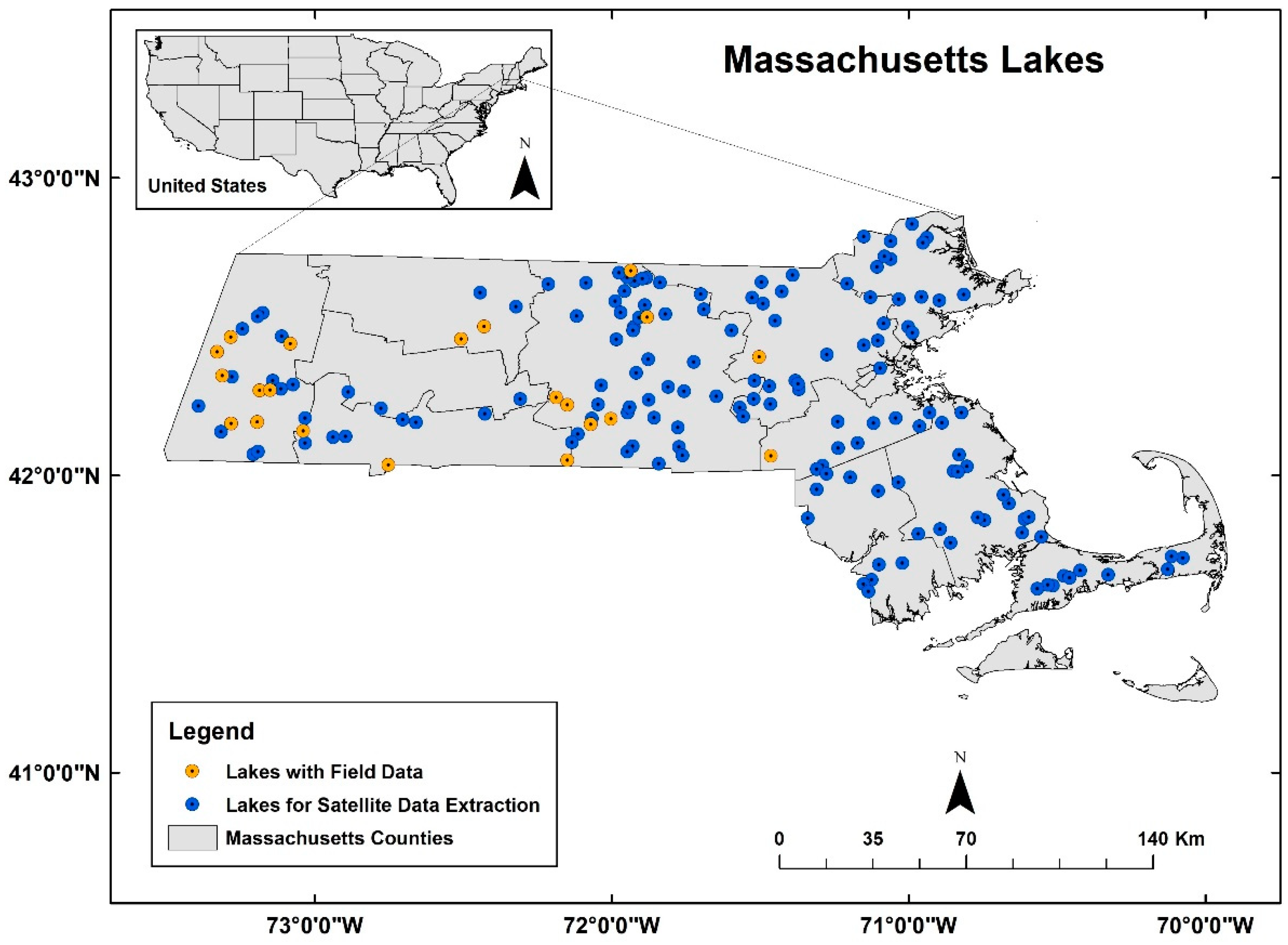
This study focused on lakes in Massachusetts, located in the northeastern United States (Figure 1). This region experiences a humid continental climate with warm, wet summers and cold, snowy winters [29]. Precipitation in the region is generally evenly distributed throughout the year except for the wet season, with an annual average rainfall of 1016–1270 mm [30]. River flows in the region are typically characterized by higher flows during leaf-off periods (~November through April) and spring snowmelt and lower flows during summer months [31,32]. Natural lakes in Massachusetts fill during the high spring flows and gradually decline during the drier summer–fall months as evapotranspiration exceeds precipitation inputs [33,34]. Most WD lakes implement drawdowns in the fall by releasing water downstream when river flows are lowest. Past research indicates that the timing of these drawdowns, which coincide with the region’s seasonal precipitation and temperature patterns, can significantly impact physical habitat structure and macrophytes in Massachusetts lakes [35].
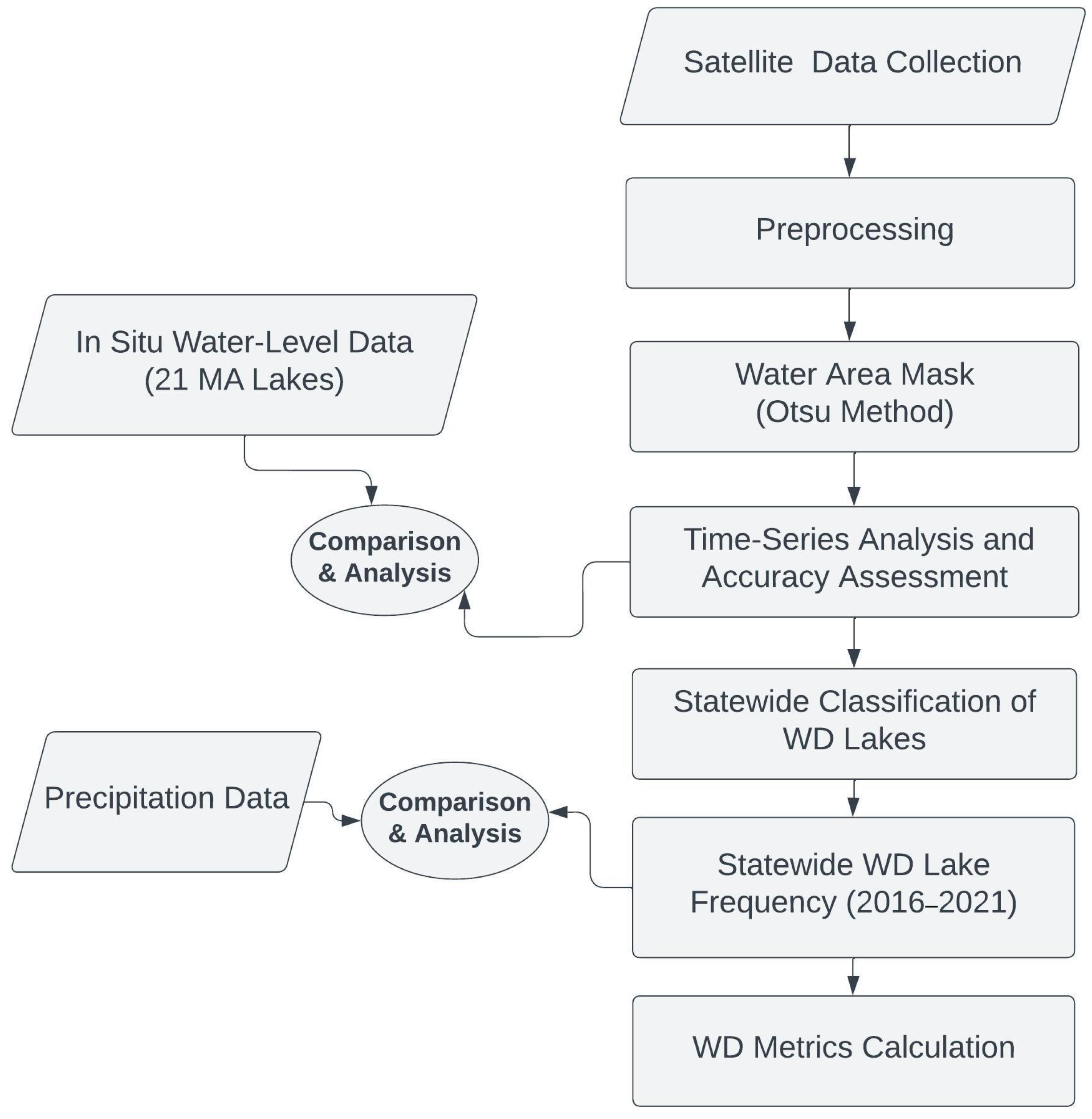
The overall methods including data collection, processing, and analysis steps involved to achieve the objectives of this study are shown in Figure 2. The detailed descriptions of each component are presented in the following subsections.

2.2. Satellite Data Collection and Preprocessing

This study utilized two optical sensors (Landsat 8-Operational Land Imager (LS8-OLI) and Sentinel 2A/B-Multi Spectral Instrument (S2-MSI)) and one SAR sensor (Sentinel 1A/B-SAR (S1-SAR)) to generate surface water area data (Table 1). To avoid the data download process, we used an online image processing platform (Google Earth Engine, GEE) to process and analyze the data derived from all three satellite sensors.
Top-of-atmosphere (TOA) reflectance (RTOA) level-1 data from both optical sensors (LS8-OLI and S2-MSI) were used as input for preprocessing within the GEE platform. For the S1-SAR sensor, C-band Ground Range Detected (GRD) raw data were already processed using the Sentinel 1 toolbox to produce calibrated, ortho-corrected scenes before they were made available to users on the Google Earth Engine platform. The preprocessing steps for optical sensors included cloud masking (for LS8-OLI and S2-MSI), resampling pixels to a common spatial resolution (30 m). The preprocessing steps for S1-SAR included spatial resampling at 30 m and speckle filtering. Both S2-MSI and S1-SAR sensors have multiple spatial resolutions and, therefore, spatial resampling was required to have a consistent spatial resolution. We resampled S1-SAR and S2-MSI pixels at a 30 m spatial resolution to have consistent comparison with respect to the LS8-OLI sensor’s spatial resolution. Cloud masking was performed using quality assurance bands available in both optical sensors.
The S1-SAR data available in GEE have two polarization modes, i.e., VV (vertical transmit/vertical receive) and VH (vertical transmit/horizontal receive). We used backscattering coefficients (dB) from only VV polarization mode because previous studies have found VV mode more suitable for surface water classification than VH mode [36]. SAR sensors like the Sentinel 1 emit microwave pulses and measure the intensity of backscattered energy returning to the sensor. The strength of the backscatter signal depends on surface properties like roughness, moisture content, and structure [37,38]. For open water bodies like lakes, the smooth surface acts as a specular reflector that reflects most of the incident radar pulses away from the sensor, resulting in a very low backscatter and dark tone in SAR imagery [39]. In contrast, vegetation, urban areas, and bare land have higher surface roughness, leading to diffuse scattering of radar pulses in multiple directions, including back to the sensor [40], resulting in higher backscatter intensity and brighter tone compared to water. The raw S1-SAR data contain speckle noises which may result in misclassification of water area. To remove the speckle noises, a 100 m circular buffer was used within the GEE platform and pixels within that buffer were averaged.

2.3. Water Area Mask (Otsu Method)

Following preprocessing, we used an automated surface water classification algorithm known as “Otsu” [41] to classify water and non-water regions. The Otsu algorithm is an unsupervised method that was originally developed to select a threshold for the reduction of a gray-scale image to a binary image containing two classes. The Otsu method is a complex, iterative process that selects an optimal threshold value separating two classes so that the between-class variance is maximized. To implement Otsu thresholding efficiently, we utilized JavaScript code developed by Zhou et al. [42] within the GEE platform. The code implements the Otsu method in a simplified and efficient way by using the following steps: (a) it converts the input image to a gray-scale image and calculates the histogram of pixel values; (b) it iterates over all possible threshold values and computes the between-class variance for each value; and (c) it selects the threshold value that maximizes the between-class variance and returns it as the optimal threshold. The code simplifies the original algorithm by avoiding the use of complex mathematical formulas and matrix operations. Instead, it leverages the built-in functions of the Google Earth Engine platform, such as ee.Image.reduceRegion and ee.Image.select, which are optimized for large-scale image processing. The Otsu code by Zhou et al. [42] was written for S1-SAR data and, thus, we modified the Otsu code for optical sensors (LS8-OLI and S2-MSI) using the short-wave infrared (SWIR) band as input image. In the SWIR band, water absorbs the incoming solar light strongly, and a bimodal histogram is observed. In addition, the SWIR band is also less affected by turbid water and atmospheric noise compared to the near-infrared (NIR) band used in initial studies for surface water area classification. We used the optimal threshold computed by the Otsu method in a conditional expression to classify water areas below that optimal threshold value. The surface water area was derived by counting the number of water pixels and multiplying that value to each pixel area (30 m × 30 m = 0.0009 km2).

2.4. Time-Series Analysis and Accuracy Assessment

To differentiate WD and non-drawdown lakes, we extracted surface water area time-series (2016–2021) data from both optical and SAR sensors. We selected 2016–2021 for data extraction because data from both optical and SAR sensors were available during this period, allowing us to compare the time-series results from all three sensors (LS8-OLI, S2-MSI, and S1-SAR). Using these three sensors, we compared the trend between satellite-derived surface water area and in situ water level. We used all the available common dates between satellite and in situ data to compare surface water area time series derived from satellite data and 24 h mean in situ water-level data for 21 MA lakes. To compare in situ water-level data with satellite-derived surface water area, bihourly water-level data were averaged for 24 h to obtain the mean daily water level.
To assess accuracy, we first found the total number of matched dates between the available satellite images and in situ logger data during the study period for each of the 21 lakes. We then qualitatively examined the alignment in the patterns and trends between the satellite-derived surface water area time series and the in situ water-level time series. We looked for consistent increases and decreases that aligned between the two datasets, indicative of accurate capture of water-level fluctuations. We assessed accuracy of the satellite data by comparing the magnitude and spatiotemporal trend of surface water area to those of in situ relative water-level data. In situ water-level data were available from 18 WD lakes and 3 non-drawdown (ND) lakes in MA (Figure 2; [2]). Lakes varied in surface area (0.19–4.21 km2), mean depth (1.5–7.6 m), and maximum depth (3.0–25.7 m). The data were collected using pressure transducers (Onset HOBO U20L-01, Bourne, MA) bihourly for 3–4 years (2014–2018). More details on in situ water-level data can be found in Carmignani et al. [2].
We assessed how lake size, shape, and shoreline slope affected the surface water area trend when compared to in situ water-level time-series data. Some lakes were very narrow in shape (Hamilton), some with dendritic geometry (Wyman) and some with wide surface area (Stockbridge, Richmond, Wyola). For shoreline slope, we used digital bathymetry maps of lakes (Supplementary Materials Figure S1) to interpret the surface water area fluctuation observed in satellite maps. Surface water spatiotemporal maps were produced in the GEE platform for selective WD lakes before, during, and after winter drawdown.

2.5. Statewide Classification of WD Lakes

Using the US Fish and Wildlife Service National Wetland shapefile of lakes, we extracted surface water area data from October 2014 to October 2021 for all MA lakes >0.3 km2 (166 lakes) using S1-SAR data in the GEE platform. We empirically determined the 0.3 km2 threshold by evaluating the accuracy of the satellite-derived water area measurements against in situ water-level data for a subset of MA lakes ranging in size from 0.1 km2 to 15 km2. Other studies have also found that accuracy of satellite-based lake water area extraction decreases for smaller water bodies without specifying any size threshold [43,44,45]. While the 0.3 km2 cutoff was suitable for reliably monitoring water level fluctuations in our MA lake dataset, further accuracy assessments would be required to determine an appropriate minimum lake size threshold if applying this method in other geographic regions. After applying the 0.3 km2 cutoff, we exported the time-series surface water area data from the GEE platform in .csv format for further analysis.
To differentiate WD lakes from ND lakes, Carmignani et al. [2] divided each annual cycle (April to March) of in situ water-level data into summer (April to September) and winter (October to March) periods. They found that WD lakes exhibited significantly lower water levels during the winter compared to summer, while ND lakes showed the opposite seasonal pattern. We implemented a similar seasonality-based classification idea in an automated way using a machine learning technique which takes time-series data as input to classify WD lakes. We used K-nearest neighbor (KNN) to classify the time series of WD and ND lakes. This method can handle large datasets and automates the WD lake characterization process. To implement this classification algorithm, we used a Python library package, tslearn (https://github.com/tslearn-team/tslearn, accessed on 1 December 2022).
To implement the KNN classification model, continuous time-series data were required as input. Therefore, we used linear interpolation between the actual Sentinel 1 observation dates (~6 days) to generate daily surface water extent values for each lake. This allowed creation of a consistent time-step series across all lakes for model implementation. While interpolation introduces some uncertainty on days without true observations, we chose linear interpolation as a simple method to create a continuous dataset while minimizing assumption of non-linear changes between observations. Importantly, the ~6 days revisit frequency still captured the major seasonal fluctuations in water levels critical for distinguishing winter drawdown. We excluded outliers in the time-series data using a 95% confidence interval and standardized the data using a normalization method (min–max).
To classify the lakes with in situ data, we used a 7-fold cross validation approach to maximize the data for model training. We used a stratified sampling approach based on the WD and ND classes of the lakes to ensure a balanced representation of both classes in the training and testing datasets. Out of 44 WD lake samples (10 lakes × 2 yrs = 20; 8 lakes × 3 yrs = 24), we used 30 samples for training and 14 samples for testing. Out of eight ND lake samples (2 lakes × 3 yrs = 6; 1 lake × 2 yrs = 2), we used five samples for training and three samples for testing. Cross-validation was performed using the test dataset (WD = 14, ND = 3) in seven iterations. We divided the test dataset of 17 total lakes (WD = 14, ND = 3) into 7 groups, each containing 3 lakes (2 WD and 1 ND lake). For each fold, the 3 lakes were held out for model testing while the remaining 14 lakes were used for model training. In each iteration, we used 49 samples for training and 3 samples for testing. We used different test samples in each of the seven iterations to cover all test samples. The accuracy results were then averaged across the seven folds. We also examined the effect of the time window on classification accuracy. Time windows included 12 months, 6 months (August to December), and 3 months (October to December). We followed the same procedure: three test samples at a time and averaging the accuracy across seven iterations for the time-window experiments.
For satellite data classification, we selected 38 known lakes (WD = 24; ND = 14) with either WD history or no history of WD based on a survey result conducted by Carmignani et al. [2]. We used 5 years (April 2016–March 2021) of surface water area time-series data for training and testing the accuracy of the classification model. For training, we used a total of 140 samples (WD = 90 samples (18 lakes × 5 yrs); ND = 50 samples (10 lakes × 5 yrs)) and for testing, we used a total of 50 samples (WD = 30 samples (6 lakes × 5 yrs); ND = 20 samples (4 lakes × 5 yrs)). We used a combination of lakes in both training and testing datasets to avoid any site-specific bias in the result. Similar to in situ analysis, we used 12-month, 6-month, and 3-month time series during the classification. Once we finalized the best time window for satellite-based classification, we combined the accurately classified WD and ND lakes samples from both training and testing datasets to create a master training dataset for classifying all 166 lakes in MA.
To our knowledge, this study represents the first application of machine learning techniques to satellite data for statewide mapping and classification of WD versus ND lakes. While past studies have focused on manual classification of individual or small groups of lakes, our method allowed efficient classification of drawdown status across 166 lakes in Massachusetts.

2.6. Statewide WD Lake Frequency (2016–2021) and Precipitation Data

We created a statewide WD frequency map for 166 lakes using satellite-based classification data between 2016–2021. The multi-year statewide frequency mapping provides novel insights into the spatial patterns and prevalence of winter drawdown practices not feasible through analysis of individual lakes. The annual classification for each lake was performed by implementing the ML-based time-series algorithm based on the tslearn package [46]. This algorithm can capture the shape and similarity of time-series data, but it may not account for the seasonality and trend of the data. Therefore, we applied some post-processing steps to filter out the false-positive WD lakes using the seasonality and trend information. We calculated the slope of the water level between 1 October and 1 December for each year, which is the expected period of water-level decrease for WD lakes. If the slope was positive, indicating an increasing water level, we reclassified the lake as a ND lake. We also reclassified the lakes with WD starting dates beyond 31 January as ND lakes, because winter drawdown operations usually end by the end of January. We performed these post-processing steps to improve the accuracy of classification of WD lakes. These post-processing steps were simple and easy to implement compared to complex preprocessing techniques such as deseasonalization and detrending the time-series data. In addition, WD lakes exhibit a distinct seasonal decline in water levels during fall–winter months, while ND lakes do not show this sharp downward trend. Removing the seasonal component through deseasonalization may eliminate this key differentiation in hydrologic regimes that the model uses for classification. Likewise, not detrending retains the directionality and magnitude of water-level changes that distinguish drawdown versus non-drawdown lakes. However, exploring preprocessing techniques as an option to potentially improve classification is an area for future refinement.
To assess the effect of precipitation on WD frequency, precipitation data for MA were downloaded from NASA’s Giovanni web interface for 2016–2020. The GPM monthly precipitation product (GPM_3IMERGM_07) was downloaded for the entire state and then county-wide data were extracted using MA county shapefiles to exclude data from islands. We extracted both annual (12 month) precipitation and precipitation data for September to December for each of the five years.

2.7. WD Metrics Calculation

A unique aspect of this study was the development of methods to automatically calculate key WD metrics including timing, duration, magnitude, and lake area exposure using satellite-derived lake water levels. Automatic calculation of these metrics allowed efficient quantification of drawdown characteristics across many lakes and years. We calculated WD metrics for each of the five years for WD lakes using the MA time-series data (see, as an example, Supplementary Materials Figure S2). To determine WD metrics, we used 1 September as the starting window to exclude any drawdown happening before this date. We used a criterion of a consistent decline in water level until it reached the lowest level to determine the start of WD. Within such a consistent decline, we derived the first date of such a consistent decline as the WD starting date. Then, to find out the relative WD magnitude, we first determined the reference pool level (RPL) for each year and the lowest magnitude during the WD phase. To determine the RPL, we used a time window of 1 week before and after the maximum value post-lowest water level and then computed the median value within that 14-day window (±1 week of maximum value). We subtracted the lowest water level from the RPL value to derive the relative WD magnitude for each lake and for each year. We considered the first time when the water level reached the RPL after WD as the end of WD. WD duration was calculated as the difference between the end of WD and the start of WD. Finally, we computed the percentage of lake area exposed (%LAE) during the WD phase as Equation (1). We created boxplots for each metric across five years to show the annual variability as well as the variability across WD lakes. Correlation analysis was also used to show relationships among metrics and variability within and across years.
% L A E = W A   R P L W A   ( L o w e s t   l e v e l ) W A   ( R P L ) × 100
where %LAE = percentage of lake area exposed at lowest water level, WA (RPL) = water area at reference pool level, and WA (Lowest level) = water area at the lowest winter water level.

3. Results

3.1. Surface Water Area (Optical vs. SAR)

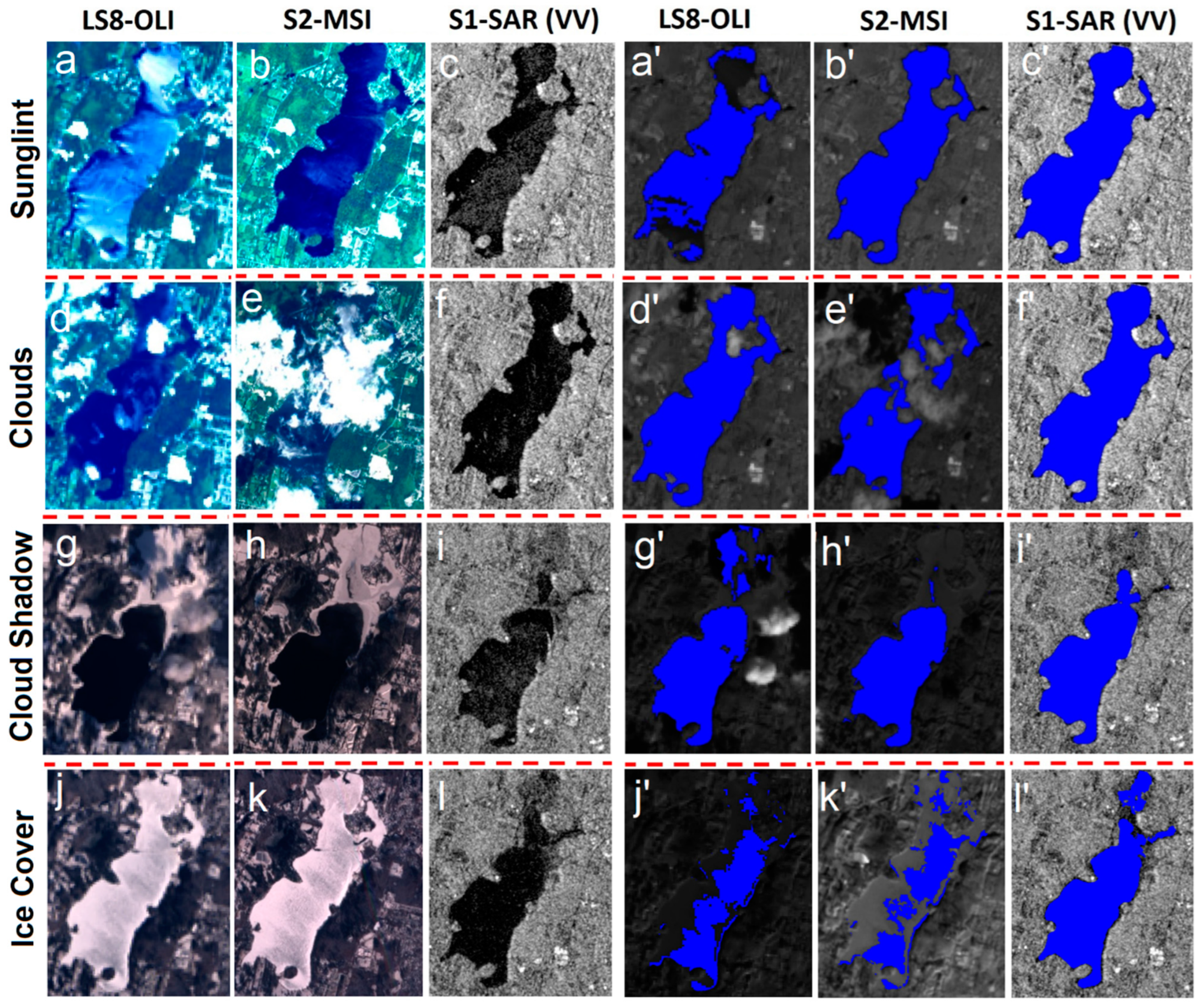
Comparisons between surface water area values derived from optical sensors (LS8-OLI and S2-MSI) and the S1-SAR sensor revealed the effects of sun glint, cloud cover, and ice cover. LS8-OLI was affected by heavy sun glint (a mirror-type reflection) [47], such that the derived water surface area was much lower, as seen on 12 June 2017 (Figure 3a,a’). In contrast, S2-MSI and S1-SAR were not affected by sun glint on that day, allowing for a complete surface water area to be captured (Figure 3b’,c’).
Cloud cover partially affected the LS8-OLI scene (Figure 3d) and significantly affected the S2-MSI scene (Figure 3e) as shown on 30 July 2017, leading to inaccurate estimates of water area. In contrast, S1-SAR-derived surface water extent was not affected by clouds (Figure 3f’). Cloud shadow and ice cover were observed in LS8-OLI and S2-MSI scenes acquired on 14 December 2017 (Figure 3g,h). The cloud-affected region in the LS8-OLI scene was misclassified as water (Figure 3g’) and ice cover significantly reduced the surface water area derived from both optical sensors (Figure 3g’,h’). In case of SAR imagery (Figure 3i), we observed that the ice-covered region appeared grey and water appeared dark; therefore, only the dark region was classified as water (Figure 3i’). Further, when the lake was completely covered by ice in 31 January 2018 scenes (both LS8-OLI and S2-MSI) (Figure 3j,k), water area values derived from optical sensors were very low (Figure 3j’,k’). However, for the same date, S1-SAR-derived water area was much higher than that derived by optical sensors and almost the entire lake had water except for the northern part (Figure 3l’).
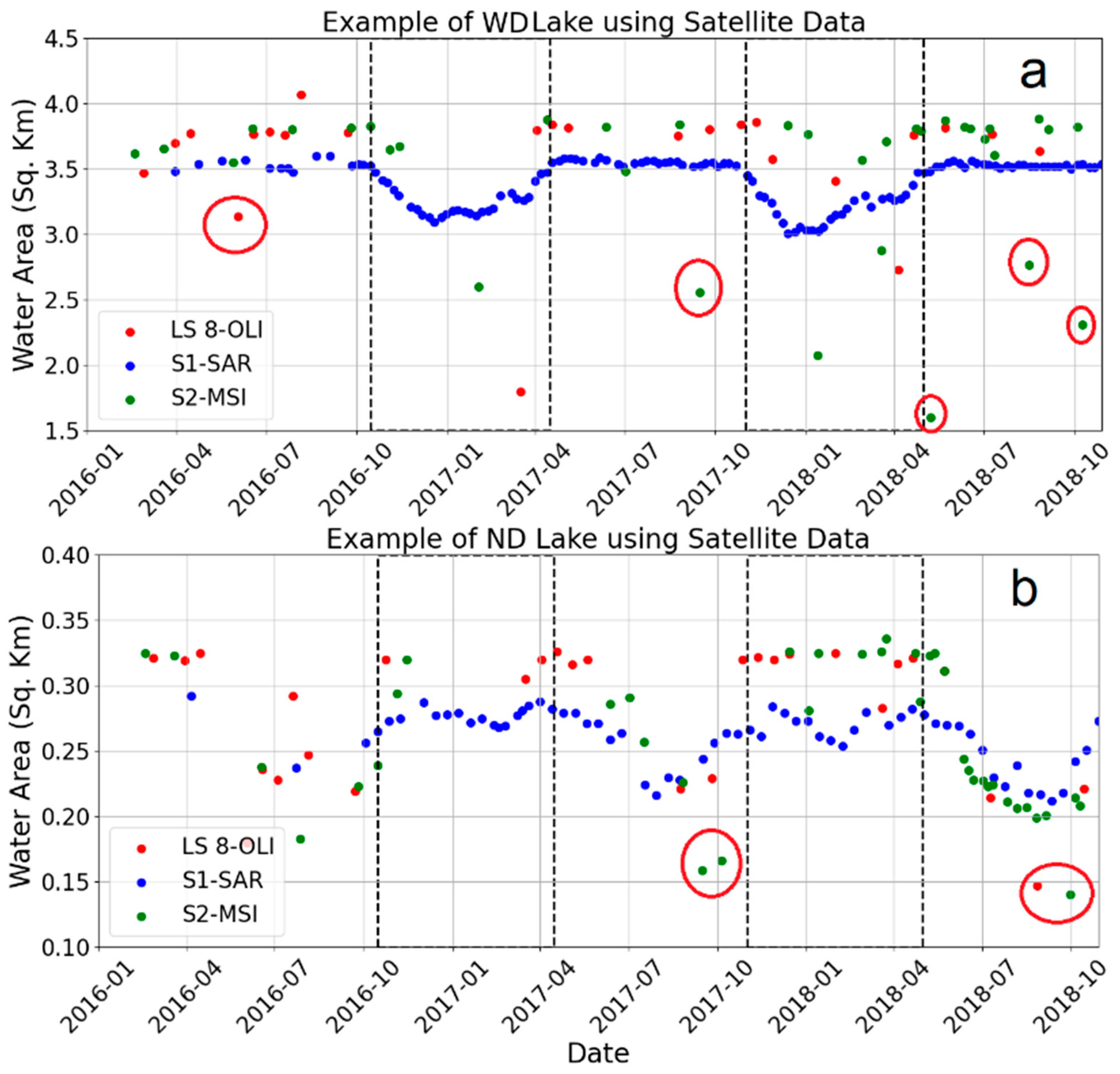
The time-series analysis revealed that cloud and ice problems limit the use of optical sensors to differentiate between WD and ND lakes (Figure 4). This was evident in the comparative time-series example of WD and ND lake surface water area derived from three sensors (Figure 4). There was a data gap and implausible values (marked in red circles in Figure 4a,b) in surface water area derived from optical sensors due to partial cloud cover and ice cover over the study area. In contrast, surface water areas derived from the S1-SAR sensor showed a clear and consistent trend (Figure 4). For a WD lake, the gradual reduction in surface water area was observed in late fall and it came back to normal before the summer (Figure 4a). For a ND lake, surface water area was observed to be lowest during summer and highest during the wet season as expected in case of a natural lake (Figure 4b).

3.2. Surface Water Area vs. In Situ Water Level

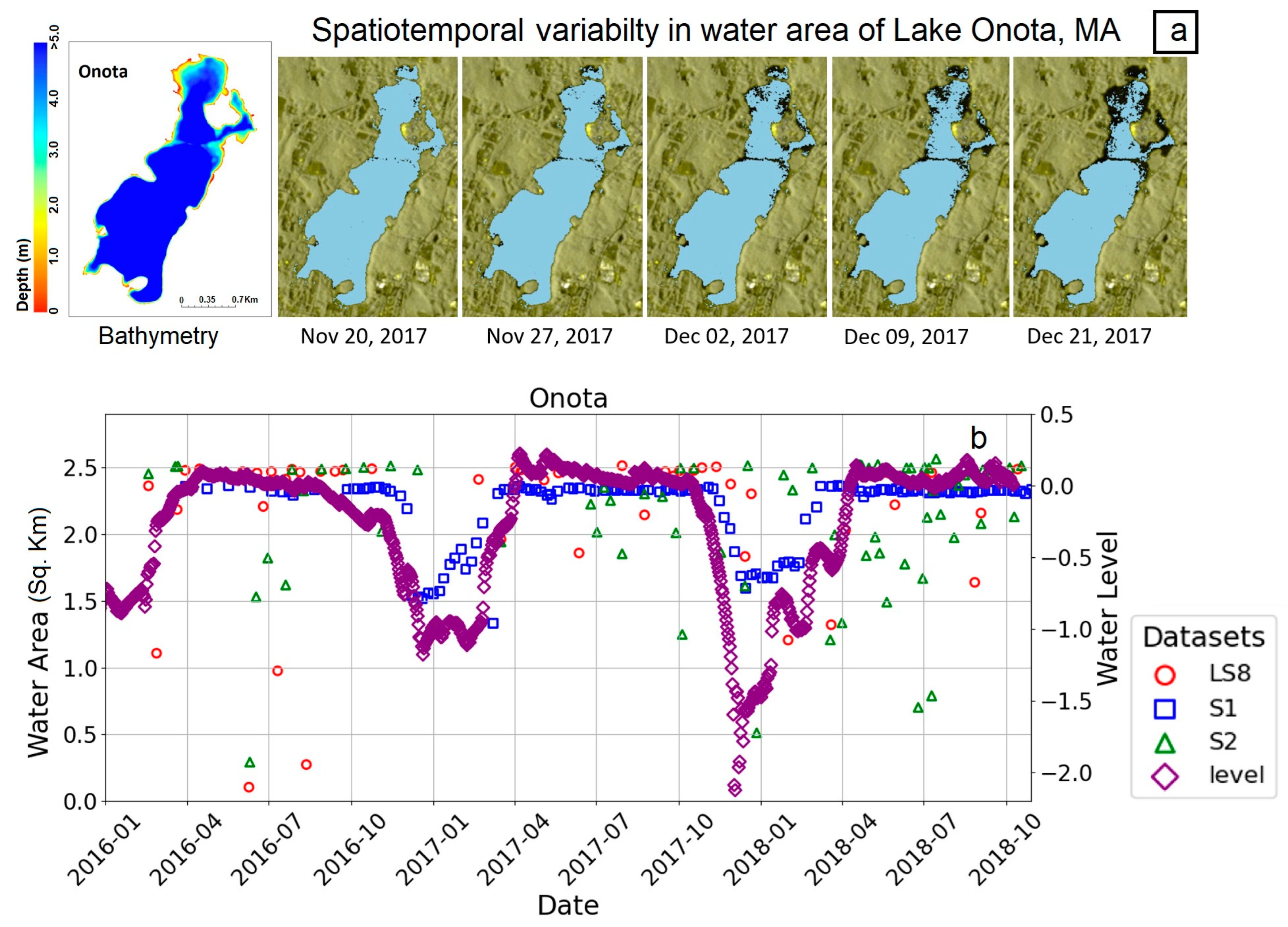
S1-SAR-derived spatiotemporal maps corresponding to Lake Onota, a WD lake, showed consistent decline in water area during WD period (Figure 5a). The areas exposed due to WD were mainly the shallowest regions within the lake, as indicated when compared with a bathymetry map (Figure 5a). Comparative analysis of three sensors indicated the highest match-up data points with in situ water-level data were obtained using the S1-SAR sensor. This was in contrast to limited data from optical sensors due to cloud cover and the longer revisit frequency of LS8-OLI (16-days) (Figure 5b). Additionally, observing the recession and refill trend for WD lakes proved challenging with sparse observations from optical sensors. In addition, distinguishing lower water levels due to WD or due to partial cloud cover or ice cover was not easy in time-series data derived from optical sensors. In contrast, S1-SAR-derived time-series data clearly showed the recession and refill trend for WD lakes similar to those of in situ observations (Figure 5b). Based on these results and the aforementioned limitations of optical sensors, we did not include them in further analysis and only data and results from the S1-SAR sensor were analyzed.
Relative water levels derived from in situ loggers for 21 MA lakes and surface water area derived from the S1-SAR sensor showed similar patterns in time series for several large- and medium-sized (Supplementary Materials Figure S3) lakes. For a few large lakes, satellite-derived data were not well aligned with in situ water-level data. We also observed a time lag between in situ water level and satellite-derived surface water area, whereby during fall drawdown, in situ water level declines precede satellite-derived water area declines. Conversely, during recession, we observed that satellite-derived surface water area returned to normal levels earlier than in situ water levels. The smallest lake size that showed similar water-level fluctuations as those of in situ data among WD lakes was Lake Greenwater (0.31 km2). The smallest ND lake which showed a similar pattern as that of in situ data was Leverett Pond (0.3 km2). Therefore, we decided to use this size threshold (0.3 km2) for extracting statewide lake data for characterizing WD lakes using S1-SAR data.

3.3. Classification of WD Lakes

The in situ ML-based time-series classification results showed the highest overall accuracy for both training (99.49%) and testing (95.83%) datasets (Table 2) when we used a 3-month time window (October to December), as opposed to 12- and 6-month time windows (Table 2). In addition, individual accuracy for both WD training (99.7%) and WD testing (100%) as well as ND training (98.21%) and ND testing (87.5%) was observed to be highest for a 3-month time window compared to 6-month and 12-month time windows (Table 2). These results suggest that the 3 months from October to December are crucial for differentiating WD and ND lakes in MA.
The ML-based time-series classification using satellite data showed the highest overall classification accuracy (83.57%) for the training dataset using a 3-month time window (October to December), compared to 6-month and 12-month windows (Table 3). However, overall accuracy for the testing dataset was observed to be highest (62%) using a 12-month time-window (Table 3). For individual lake types, the classification accuracy of the training dataset for both WD and ND was highest for the 3-month time window. However, for the test dataset, accuracy of WD classification was reduced when using a 3-month time window (76.66%) compared to a 12-month time window (86.67%). The accuracy for the ND test dataset was low for 12-month and 6-month time windows (25%) and accuracy slightly increased (35%) when using a 3-month time-window. Overall, there are more chances of false positives (ND lake classified as WD lake) compared to false negatives (WD lake classified as ND lake) using this ML-based classification (Table 3).
To improve the accuracy of the satellite-based classification implemented on the statewide dataset, we combined both training and testing data for both WD and ND lakes (WD: 120; ND: 70). However, we excluded some problematic lake data with random fluctuations (WD: n = 20; ND: n = 19) which resulted in a final training dataset of 151 samples (WD: n = 100; ND: n = 51; Total: n = 151). This new training dataset resulted in improved accuracy for both WD (98.0%) and ND (98.0%) classification using a 3-month (October to December) time window.

3.4. Statewide WD Classification

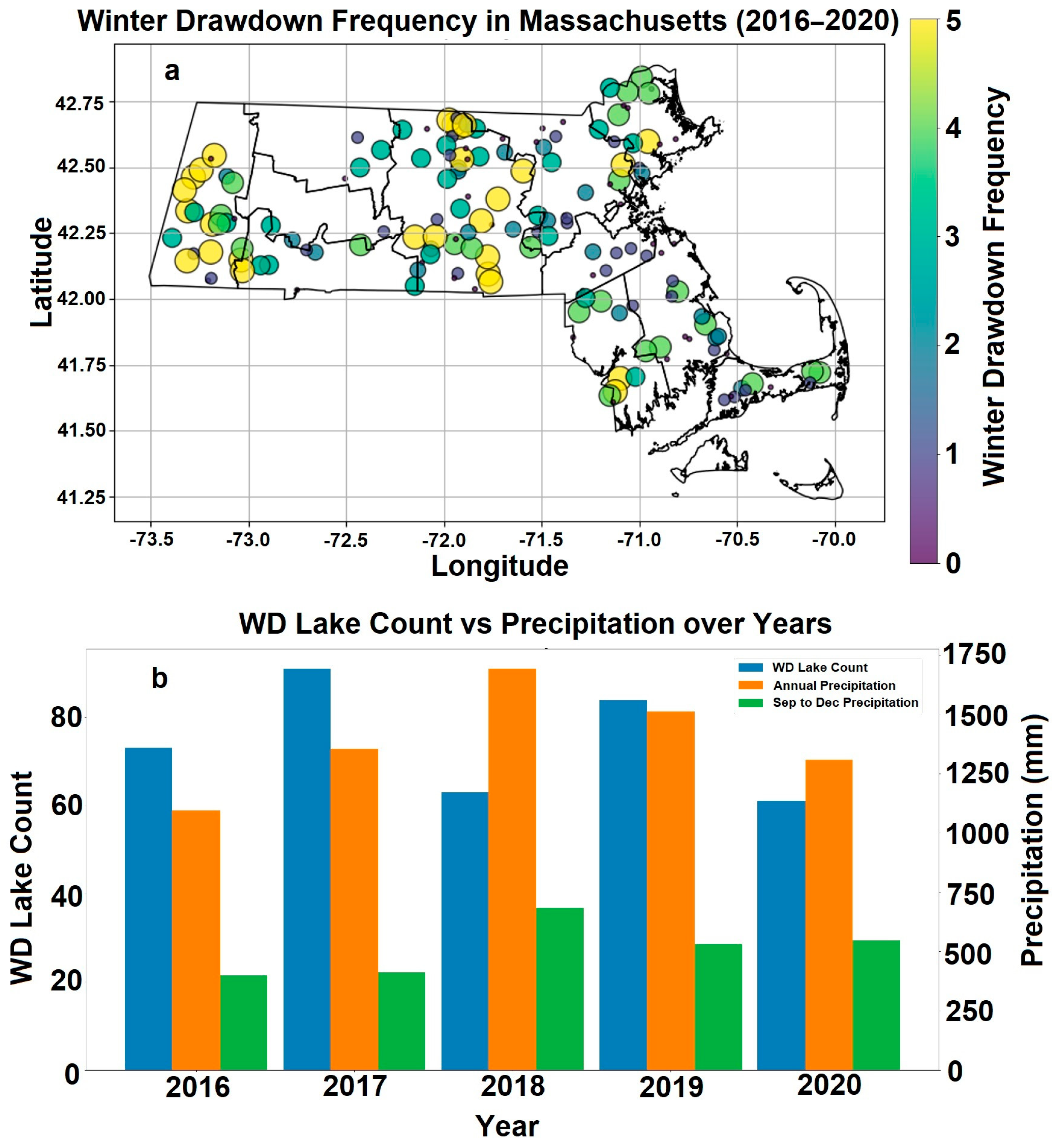
WD is widely practiced throughout MA, with the most frequent drawdowns happening in the western and central parts of the state (Figure 6a, Supplementary Materials Table S1). Out of 166 lakes, 51 are noted for conducting WD annually (≥4 years classified as WD) and 24 lakes conduct WD biennially. The total count of WD lakes in yearly classification across MA showed an alternative pattern, with a higher number of WD lakes in 2017 and 2019 compared to the other three years (Figure 6b). Over the same period, annual and fall precipitation was highest in 2018 and lowest in 2016 and 2020 (Figure 6b).

3.5. Winter Drawdown Metrics

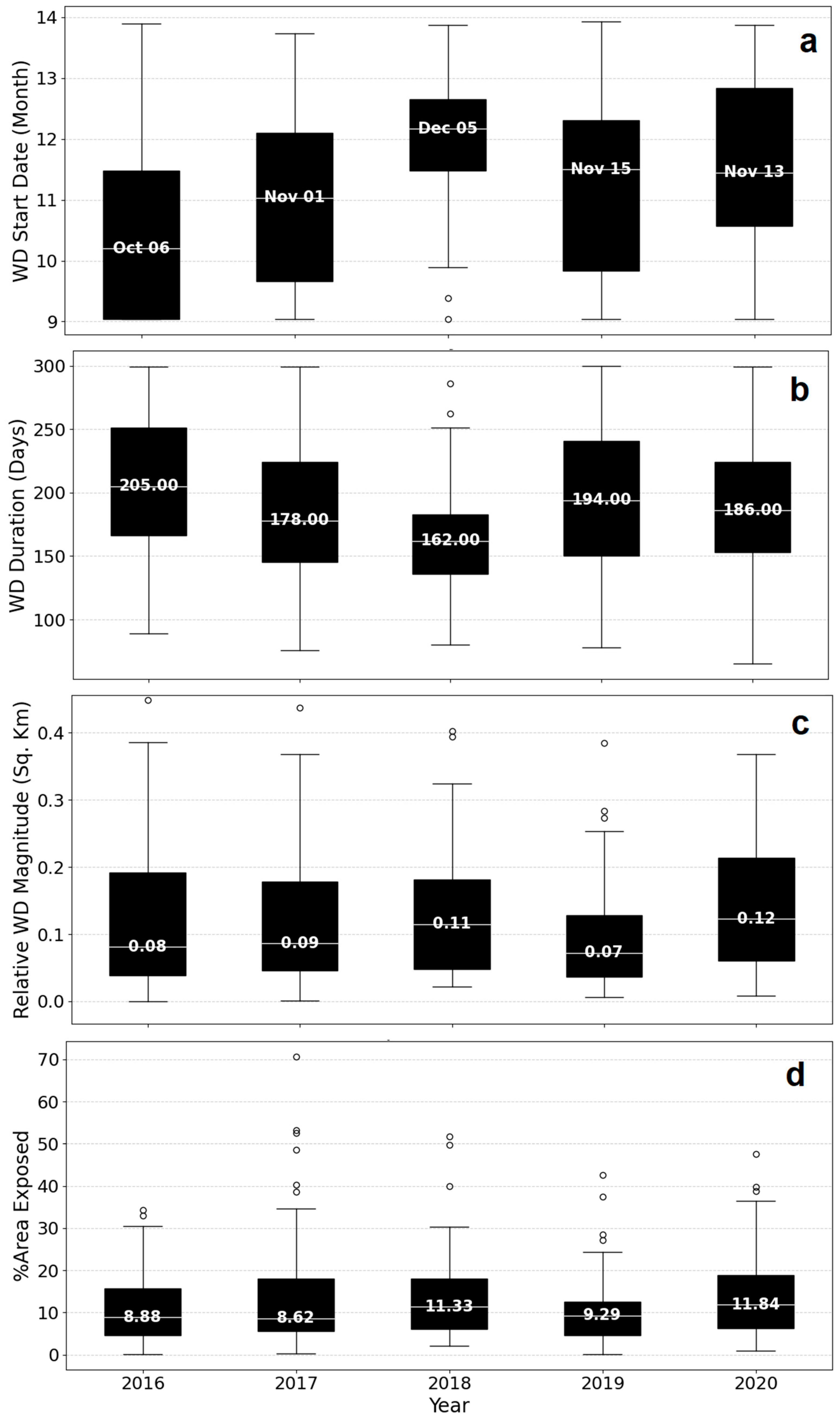
Boxplots revealed the interannual variability in WD metrics (Figure 7). The median WD start date was earliest in 2016 (6 October) and latest in 2018 (5 December), with the smallest variability (interquartile range (IQR) = 35 d; σ = ±31 d) in 2018, the wettest year of the 5-year period (Figure 6b; Table 4). Correspondingly, the longest WD duration was in 2016 (median = 205 d) and the shortest duration was in 2018 (median = 162 d; Figure 7b). In 2018, both WD start date and duration had the narrowest interquartile range (WD start date IQR = 35 d; WD duration IQR = 47 d) compared to during the other 4 years (Table 4).
We observed that the median WD magnitude increased between 2016 (0.08 km2) and 2018 (0.11 km2). It should be noted that the median size of the 166 lakes under this study was 0.81 km2. The maximum WD magnitude (7.55 km2) and variability in WD magnitude among lakes were highest in 2018 (σ = ±1.13 km2) (Table 4), the year with the highest precipitation in the 5-year study period (2016–2020). Following the wet year of 2018, precipitation decreased in 2019. Correspondingly, we observed a decline in median WD magnitude that year (Figure 7c). In fact, 2019 had the lowest median WD magnitude (0.07 km2) as well as the lowest variability (IQR = 0.09 km2; σ = ±0.12 km2) in WD magnitude among the studied lakes. However, when precipitation further decreased in 2020, we did not observe a continued decline in WD magnitude. Instead, median WD magnitude increased in 2020 despite the reduction in precipitation. The median percent area exposed ranged from 8.6% (2017) to 11.8% (2020), although there were high outliers each year (Figure 7d). As with WD magnitude, the lowest variability in lake area exposure occurred in 2019 (IQR = 7.99%; σ = ±7.60%) (Table 4). The median lake area exposure was also lowest in 2019 (9.29%), mirroring the median WD magnitude.
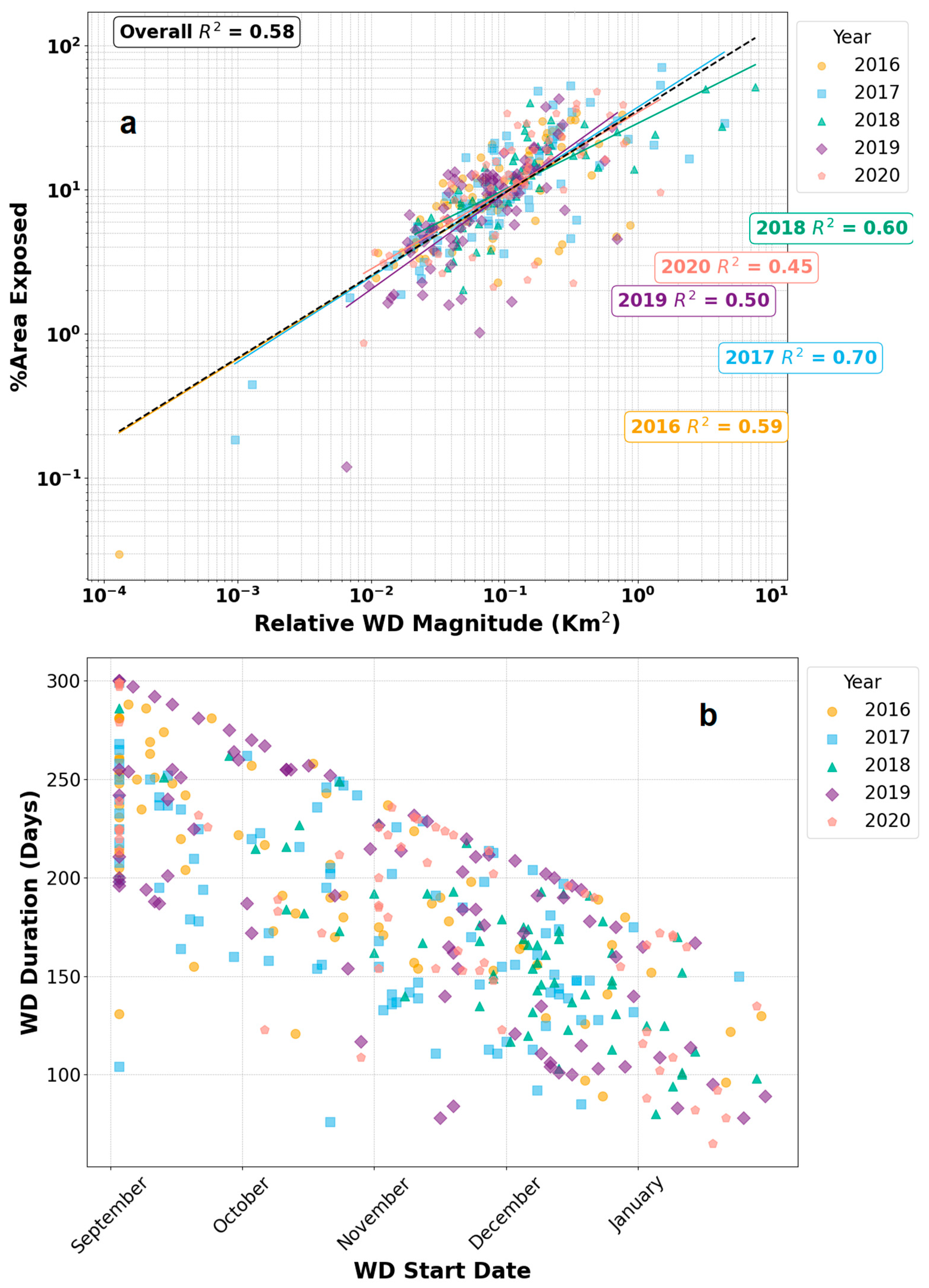
Relative WD magnitude was positively correlated with % lake area exposed (Figure 8a). The weakest relationship (R2 = 0.45) occurred in 2020, the year with the lowest number of WD lakes, and the strongest relationship (R2 = 0.70) occurred in 2017, the year with the highest number of WD lakes. There was high cross-lake variability in both metrics, with the highest area exposed (>45%) in 2017 and 2018 (Figure 8a). Similarly, there was high cross-lake variability in WD start date and WD duration (Figure 8b).

4. Discussion

Our study demonstrated the utility of freely available multi-sensor satellite data in the GEE platform for characterizing winter water-level drawdowns across lakes in Massachusetts. Among the three sensors compared, S1-SAR provided the most consistent and gap-free time-series data to differentiate drawdown and non-drawdown lakes compared to optical sensors which were prone to cloud cover and sun glint effects. The machine learning-based time-series analysis accurately classified drawdown and non-drawdown lakes using both in situ and S1-SAR data when a 3-month period (October–December) was used. Leveraging GEE and machine learning approaches, we were able to conduct a comprehensive analysis of statewide lakes (166 lakes > 0.3 km2) and identified drawdown frequency and WD metrics over a 5-year period. Interannual variability in metrics suggested that WD is primarily a managed activity rather than driven by precipitation variability. The same approach can be extended to broader areas and regions to assess the impacts of WD on lake ecosystems and water resources.

4.1. Effectiveness of Sensors for Capturing Water Area and Water-Level Fluctuations

We conducted a robust accuracy assessment of different satellite sensors for capturing water-level variations during the challenging winter season. Our analysis identified Sentinel 1-SAR as the most reliable for capturing winter water-level variations indicative of drawdown practices. Our results demonstrated some of the major advantages of SAR over optical sensors for mapping surface water extent under problematic conditions like cloud cover, sun glint, and ice cover. Optical sensors like Landsat and Sentinel 2 have been used widely for water body mapping [48,49] but are limited by an inability to penetrate cloud cover. Several studies have shown SAR provides consistent water extraction unaffected by clouds or sunlight angle [19,26]. Our analysis matched these past findings, with frequent cloud gaps and sun glint artifacts in the Landsat and Sentinel 2 time series. SAR has also been found to better characterize lakes during ice cover compared to optical data [50,51], though accuracy declines once the lake fully freezes over [52,53,54] and it results in overestimation of water area due to specular reflection from a smooth surface. A hybrid approach incorporating optical and SAR data could help address this limitation during winter. Overall, Sentinel 1 provided consistent time-series data on surface water extent changes that served as a proxy for relative water-level fluctuations in lakes during fall drawdown and spring refill periods.
The time-series analysis of surface water extent changes derived from S1-SAR aligned well with in situ logger data. The relationship between satellite-derived surface water area and relative in situ water-level fluctuations has been assessed in multiple past studies [43,55,56]. Strong correlations are typically found for lakes with gradual slope shorelines, low shoreline-to-surface-area ratios, and well-defined boundaries [43,57]. The small discrepancies between SAR-derived area and in situ water levels could be attributed to factors such as wind, shoreline slope, frozen lake surface, size and shape of the lake, in situ data logger deployment location, and drawdown magnitude [43,57,58]. Shoreline slope influences the extent of water-level change that is detectable through area change. For instance, Figure 5b shows significantly lower areal change compared to the relative water-level fluctuation. Steeper slopes result in smaller areal changes relative to water level fluctuations. Moderate sloping shorelines are more suitable for detecting gradual water-level changes [58]. Additionally, frozen lake surfaces can mask the open water–ice boundary used to estimate area as water levels decline under ice.
Busker et al. [43] observed lower accuracy for smaller waterbodies but mentioned that along with size, there are many other factors which may contribute to accuracy such as surrounding topography, surface waves, winter ice coverage, and shape of the water body. Keys and Scott [57] found that lakes with dendritic geometry resulted in poor results compared to lakes with well-defined boundaries. We also observed the effect of size, shape, and shoreline slope effect on accuracy when comparing satellite-derived results with in situ water-level measurements for 21 lakes in MA. For example, lakes with smaller size (<0.3 km2) (Cranberry Meadow, Silver, Brookhaven) showed more random fluctuations in water area and did not align with in situ water level, whereas lakes with relatively larger size (Otis, Onota, Stockbridge, Goose, Garfield, Richmond, Ashmere) aligned well with in situ water-level fluctuations. For some moderately sized lakes (0.4 to 0.9 km2) with steeper bathymetry sloping (Buel, Watatic, Quacumquasit), water area did not show a similar trend compared to that observed in in situ water levels. In addition, the nature of the shoreline bathymetric gradient can also introduce lag between satellite-derived water area and in situ water levels. This is mainly because small water-level drops may not expose much area until a certain depth threshold is crossed. We observed a time lag between the satellite-derived surface water area recovery and the in situ water-level recovery in spring (e.g., Figure 5b). This time lag varies from lake to lake based on lake size, bathymetric profile, and shoreline slope of the lakes. The primary physical reason for such variable time lag could be the in situ sensor deployment location because in situ sensors provide measurements at a discrete point location, while satellite imagery provides water area variations for overall lakes. If water levels are increasing first in shallow, near-shore regions distant from the sensor, this could introduce a lag before the in situ gauge starts to record the rising water. Lakes with dendritic geometry (Wyman, Boon) and narrow shape (Hamilton) also showed poor alignment with in situ water levels. Though there exist the above factors which may affect the accuracy of satellite-derived water-level fluctuations, nonetheless, the S1-SAR observations provided indicative relative changes in lake water levels useful for assessing winter drawdown practices.

4.2. WD Frequency in MA Lakes

Using the extracted water area time-series data, a machine learning approach was implemented to classify WD versus ND lakes based on their seasonal water-level fluctuation patterns. Using both in situ and satellite training data, the classification accuracy was highest when using just a 3-month (October–December) time window compared to longer 6- and 12-month periods. The 6-month and 12-month time window classifications could be affected by drawdown during summertime and may result in misclassification of ND lakes as WD lakes (false positive). The 3-month window (October–December) captures the active drawdown phase when water levels steadily decline in WD lakes in MA in contrast to ND lakes that show seasonal variability but not large directional changes during fall–winter months [2]. Potential uncertainty exists from the linear interpolation used to create daily water extent values between actual Sentinel 1 observation dates. Future work could incorporate methods to estimate non-linear changes during intervals between satellite observation dates. A limitation of the machine learning model’s development was the imbalance between the number of WD and ND samples available for training and testing the classification. The disproportionate sample sizes between classes may have biased the accuracy results in favor of the majority WD class. While we used cross-validation approaches to account for the imbalance, it may have introduced some bias favoring the majority WD class. Increasing the ND sample size in future could improve accuracy, particularly the false-positive rate. However, the overall accuracy achieved even with imbalance classes demonstrates the potential of machine learning for automated WD classification using remote sensing time-series data.
The statewide mapping indicated that drawdowns are widely practiced across MA. Over 75% of lakes >0.3 km2 had at least one WD during the five study years, indicating it is a common management practice. There was high interannual variability in the number of lakes conducting drawdowns each year, which cannot be explained by precipitation alone. These results concur with the findings of Carmignani et al. [2] who concluded that drawdowns are primarily based on management decisions rather than climate factors. Although our study did not survey lake managers, documented reasons for conducting drawdowns include aquatic plant control, fisheries management, infrastructure maintenance, and waterfront access [35]. Additional social surveys across private and public lake managers could provide further insights into motivations behind drawdown decisions each year.

4.3. Variability in WD Characteristics in MA Lakes

The WD metrics provide new insights into the characteristics of this artificial hydrologic alteration across MA lakes. A few studies have analyzed drawdown trends for groups of lakes in particular regions [2,59]. Some drawdown studies have calculated similar water-level metrics using in situ data [1,2], but the remote sensing-derived measurements allow assessment at broader scales. Quantifying drawdown timing, magnitude, duration, and lake exposure area provides tangible metrics for evaluating ecological impacts and comparing across years and lakes [35].
Our analysis of WD metrics revealed high interannual variability in magnitude of drawdowns and lake area exposure. We observed an interesting relationship between precipitation, water-level drawdown magnitude, and lake area exposure in studied lakes over the 5-year study period. The positive association observed between precipitation and drawdown magnitude suggests that higher rainfall leads to greater water inputs and rising lake levels prior to drawdown, subsequently enabling larger drawdowns. This is evidenced by the highest precipitation, drawdown magnitudes, and among-lake variability in 2018, followed by declines in 2019. However, the rebound in drawdown magnitude from 2019 to 2020 despite declining precipitation illustrates that other factors beyond rainfall also govern drawdown dynamics. Specifically, while precipitation governs water inputs, drawdown on lake water for irrigation, municipal use, and hydroelectric generation may drive drawdown magnitude.
In contrast to drawdown magnitude, we did not see a significant relationship between precipitation and lake area exposure during drawdowns. Exposure remained relatively stable across all five years, with the lowest exposure again in 2019. This suggests area exposure may be controlled more by the morphology of lake basins and maximum drawdown depths, rather than by precipitation inputs. Furthermore, the lack of a relationship between precipitation and lake area exposure indicates that drawdown regulations successfully maintain a consistent exposed area, despite varying water levels. Overall, our findings highlight that both climate and human factors regulate lake water balances and interact to drive interannual variation in drawdown magnitude, underscoring the complexity of predicting lake responses to future environmental change. A priority for future research could be quantifying water consumption and evaluating how shifting human demand interacts with climate to control lake water levels and ecological impacts of drawdowns. Metrics like exposure area help translate the water-level changes to a habitat context. The exposure of up to 30% of lake areas for months at a time may have ecological impacts.
Considerable interannual variability was also observed in drawdown start date and duration, which correlated with precipitation patterns. While managers ultimately decide when to lower water levels each year, total annual precipitation and specifically fall precipitation appeared to influence drawdown start date and duration. Median start date showed an increasing trend between 2016–2018 aligned with precipitation patterns. This suggests that wetter conditions could delay the onset of drawdowns. In contrast, duration declined with increasing precipitation, indicating earlier refilling of lakes in wetter years. This indicates that natural hydrologic conditions mediate aspects of drawdown implementation; however, these relationships need to be interpreted cautiously given the short five-year study period. As more satellite data become available, they can strengthen the analysis of relationships between climate, management practices, and drawdown characteristics.

4.4. Web Application Interface

To facilitate broader access and use of the satellite-derived lake characterization technique outlined in this study, we developed an interactive web application leveraging the GEE platform [60]. This interface allows users to visualize and download the remotely sensed time series of lake water areas and corresponding water-level estimates for over 10,000 lakes across the northeast and upper Midwest United States. By leveraging cloud computing capabilities, the tool provides rapid access to consistently processed satellite imagery with just a few clicks. Users can zoom to a lake of interest, specify a date range, and immediately generate plots and download data. While currently limited to partner states, the application code could be adapted to monitor additional regions. Detailed documentation on the interface capabilities, underlying methodology, and potential limitations can be accessed at this link (https://tinyurl.com/yxnernxv, accessed on 1 December 2023). Overall, this web-based decision support tool represents an innovative approach to openly share and apply the remote sensing-derived water-level data to address diverse freshwater science and management needs.
5. Conclusions

This study demonstrated a scalable approach using open-access Sentinel 1-SAR data and cloud computing tools that could be applied across large regions to map and monitor water-level fluctuations in lakes [51]. The data and analysis framework developed for MA can serve as a template for assessing drawdown practices in other parts of the world, which is not feasible with in situ monitoring alone. The ability to detect WD carries many potential management applications, such as evaluating effects on near-shore habitats and relationships to lake water quality [2,35]. The information on drawdown frequency and metrics can aid water managers and policy makers in setting guidelines for balancing the intended benefits of drawdowns for nuisance plant control and infrastructure protection versus the potential ecological impacts of these artificial water-level manipulations [9]. The interactive web interface developed through this project provides state agencies and other stakeholders with a user-friendly tool to visualize drawdown frequency and characteristics. Overall, this study produced new hydrologic intelligence to inform water resource management and policy decisions related to drawdown practices.

Supplementary Materials

The following supporting information can be downloaded at: https://www.mdpi.com/article/10.3390/rs16060947/s1, Figure S1: Bathymetry map of 18 Winter Drawdown (WD) and 3 Non-Drawdown (ND) lakes (Quacumquasit, Leverett, and Congamond) within Massachusetts. The red color areas are shallowest regions and blue color areas are deepest regions within the lakes, Figure S2: Example of water area fluctuation in Lake Onota to compute winter drawdown (WD) metrics (Start of WD, End of WD, Magnitude of WD). Reference pool level is marked by dashed orange line, start of WD is marked by red dashed line, the lowest water area is marked by black dashed line, and end of WD is marked by purple dashed line, Figure S3: Comparison between in situ water level (blue) and Sentinel 1-Synthetic Aperture Radar (SAR) derived surface water area time-series (black) corresponding to the 18 Winter Drawdown (WD) lakes (a–r) and 3 non-WD lakes (s–u) for January 2016 to October 2018, Table S1: Satellite-based classification of 166 lakes >0.3 Km2 in Massachusetts for 5 years (2016–2020). Here ‘1’ represents a lake classified as winter drawdown and ‘0’ represents a lake classified as non-winter drawdown in respective 5-years (2016–2020). Latitude and longitude are for the lake outlet.

Author Contributions

A.K.: Conceptualization, Methodology, Software, Satellite Data extraction, Formal Analysis, Writing—original draft, review and editing, Visualization. A.H.R.: Project administration, Supervision, Funding acquisition, Field data curation, Writing—review and editing. K.M.A.: Project administration, Supervision, Writing—review and editing. X.H.: Methodology refinement, Writing—review and editing. C.B.: Project administration, Writing—review and editing. All authors have read and agreed to the published version of the manuscript.

Funding

This research was funded by the U.S. Geological Survey Northeast Climate Adaptation Science Center under Grant/Cooperative Agreement No. G20AC00354.

Data Availability Statement

The satellite data from Landsat, Sentinel 1, and Sentinel 2 are available via public archives from USGS and Copernicus. These satellite data can also be accessed using the Google Earth Engine platform. Precipitation data can be accessed using NASA’s Giovanni web-based application interface. The in situ lake level data used in this study are available from ScienceBase (https://www.sciencebase.gov/catalog/item/64b1760fd34e70357a2a0133, accessed on 1 December 2023). Lake bathymetry data can be accessed via Mass Wildlife (https://www.mass.gov/orgs/division-of-fisheries-and-wildlife, accessed on 14 January 2024). The lake boundary shapefile used for spatial analysis is from the US Fish and Wildlife Service National Wetland Inventory, available at (https://www.fws.gov/program/national-wetlands-inventory/download-state-wetlands-data, accessed on 14 January 2024). Satellite data and codes used in this study are available in a public repository at (https://gitlab.com/gee_codes/winter-drawdown, accessed on 15 February 2024).

Acknowledgments

This study was funded by the US Geological Survey, Northeast Climate Adaptation Science Center (G20AC00354). The authors thank all of our project partners for providing valuable suggestions and insights throughout the project. We especially thank J. Carmignani, J. Stolarski, and T. Richards from the Massachusetts Division of Fisheries and Wildlife for providing in situ data, feedback on the approach, and input on the management implications. Samuel Weber provided in-kind support to fix problems during the satellite data extraction process. Any use of trade, firm, or product names is for descriptive purposes only and does not imply endorsement by the US Government.

Conflicts of Interest

The authors declare no conflicts of interest.

References

  1. Fergus, C.E.; Brooks, J.R.; Kaufmann, P.R.; Herlihy, A.T.; Pollard, A.I.; Weber, M.H.; Paulsen, S.G. Lake water levels and associated hydrologic characteristics in the conterminous U.S. JAWRA J. Am. Water Resour. Assoc. 2020, 56, 450–471. [Google Scholar] [CrossRef] [PubMed]
  2. Carmignani, J.R.; Roy, A.H.; Stolarski, J.T.; Richards, T. Hydrology of annual winter water level drawdown regimes in recreational lakes of Massachusetts, United States. Lake Reserv. Manag. 2021, 37, 339–359. [Google Scholar] [CrossRef]
  3. Hofmann, H.; Lorke, A.; Peeters, F. Temporal scales of water-level fluctuations in lakes and their ecological implications. Hydrobiologia 2008, 613, 85–96. [Google Scholar] [CrossRef]
  4. Turner, K.W.; Wolfe, B.B.; Edwards, T.W.D.; Lantz, T.C.; Hall, R.I.; Larocque, G. Controls on water balance of shallow thermokarst lakes and their relations with catchment characteristics: A multi-year, landscape-scale assessment based on water isotope tracers and remote sensing in Old Crow Flats, Yukon (Canada). Glob. Chang. Biol. 2014, 20, 1585–1603. [Google Scholar] [CrossRef]
  5. Doubek, J.P.; Carey, C.C. Catchment, morphometric, and water quality characteristics differ between reservoirs and naturally formed lakes on a latitudinal gradient in the conterminous United States. Inland Waters 2017, 7, 171–180. [Google Scholar] [CrossRef]
  6. Cott, P.A.; Sibley, P.K.; Somers, W.M.; Lilly, M.R.; Gordon, A.M. A review of water level fluctuations on aquatic biota with an emphasis on fishes in ice-covered lakes. JAWRA J. Am. Water Resour. Assoc. 2008, 44, 343–359. [Google Scholar] [CrossRef]
  7. Kennedy, R.H. Toward integration in reservoir management. Lake Reserv. Manag. 2005, 21, 128–138. [Google Scholar] [CrossRef]
  8. Hellsten, S.K. Environmental factors related to water level regulation—A comparative study in northern Finland. Boreal Environ. Res. 1997, 2, 345–367. [Google Scholar]
  9. Mattson, M.D.; Godfrey, P.J.; Barletta, R.A.; Aiello, A. Eutrophication and Aquatic Plant Management in Massachusetts Final Generic Environmental Impact Report; Executive Office of Environmental Affairs Commonwealth of Massachusetts: Amherst, MA, USA, 2004. Available online: https://www.mass.gov/doc/final-generic-environmental-impact-report-main-document/download (accessed on 17 March 2022).
  10. Zohary, T.; Ostrovsky, I. Ecological impacts of excessive water level fluctuations in stratified freshwater lakes. Inland Waters 2011, 1, 47–59. [Google Scholar] [CrossRef]
  11. Carmignani, J.R.; Roy, A.H. Ecological impacts of winter water level drawdowns on lake littoral zones: A review. Aquat. Sci. 2017, 79, 803–824. [Google Scholar] [CrossRef]
  12. Mjelde, M.; Hellsten, S.; Ecke, F. A water level drawdown index for aquatic macrophytes in Nordic lakes. Hydrobiologia 2013, 704, 141–151. [Google Scholar] [CrossRef]
  13. Du, Y.; Zhang, Y.; Ling, F.; Wang, Q.; Li, W.; Li, X. Water bodies’ mapping from sentinel-2 imagery with modified normalized difference water index at 10-m spatial resolution produced by sharpening the swir band. Remote Sens. 2016, 8, 354. [Google Scholar] [CrossRef]
  14. Bangira, T.; Alfieri, S.M.; Menenti, M.; Van Niekerk, A. Comparing thresholding with machine learning classifiers for mapping complex water. Remote Sens. 2019, 11, 1351. [Google Scholar] [CrossRef]
  15. Nielsen, K.; Andersen, O.B.; Ranndal, H. Validation of sentinel-3a based lake level over us and canada. Remote Sens. 2020, 12, 2835. [Google Scholar] [CrossRef]
  16. Kittel, C.M.M.; Jiang, L.; Tøttrup, C.; Bauer-Gottwein, P. Sentinel-3 radar altimetry for river monitoring—A catchment-scale evaluation of satellite water surface elevation from Sentinel-3A and Sentinel-3B. Hydrol. Earth Syst. Sci. 2021, 25, 333–357. [Google Scholar] [CrossRef]
  17. Schlaffer, S.; Chini, M.; Dettmering, D.; Wagner, W. Mapping wetlands in zambia using seasonal backscatter signatures derived from envisat asar time series. Remote Sens. 2016, 8, 402. [Google Scholar] [CrossRef]
  18. Yang, X.; Zhao, S.; Qin, X.; Zhao, N.; Liang, L. Mapping of urban surface water bodies from sentinel-2 msi imagery at 10 m resolution via ndwi-based image sharpening. Remote Sens. 2017, 9, 596. [Google Scholar] [CrossRef]
  19. Pham-Duc, B.; Prigent, C.; Aires, F. Surface water monitoring within cambodia and the vietnamese mekong delta over a year, with sentinel-1 sar observations. Water 2017, 9, 366. [Google Scholar] [CrossRef]
  20. Lee, Z.; Carder, K.; Arnone, R.; He, M. Determination of primary spectral bands for remote sensing of aquatic environments. Sensors 2007, 7, 3428–3441. [Google Scholar] [CrossRef]
  21. Gower, J.; King, S.; Borstad, G.; Brown, L. Detection of intense plankton blooms using the 709 nm band of the MERIS imaging spectrometer. Int. J. Remote Sens. 2005, 26, 2005–2012. [Google Scholar] [CrossRef]
  22. Klemas, V. Remote sensing of emergent and submerged wetlands: An overview. Int. J. Remote Sens. 2013, 34, 6286–6320. [Google Scholar] [CrossRef]
  23. McNairn, H.; Shang, J. A review of multitemporal synthetic aperture radar (Sar) for crop monitoring. In Multitemporal Remote Sensing; Ban, Y., Ed.; Springer International Publishing: Cham, Switzerland, 2016; Volume 20, pp. 317–340. [Google Scholar] [CrossRef]
  24. Marin, C.; Bertoldi, G.; Premier, V.; Callegari, M.; Brida, C.; Hürkamp, K.; Tschiersch, J.; Zebisch, M.; Notarnicola, C. Use of Sentinel-1 radar observations to evaluate snowmelt dynamics in alpine regions. Cryosphere 2020, 14, 935–956. [Google Scholar] [CrossRef]
  25. Torres, R.; Snoeij, P.; Geudtner, D.; Bibby, D.; Davidson, M.; Attema, E.; Potin, P.; Rommen, B.; Floury, N.; Brown, M.; et al. GMES Sentinel-1 mission. Remote Sens. Environ. 2012, 120, 9–24. [Google Scholar] [CrossRef]
  26. Amitrano, D.; Martino, G.; Iodice, A.; Mitidieri, F.; Papa, M.; Riccio, D.; Ruello, G. Sentinel-1 for monitoring reservoirs: A performance analysis. Remote Sens. 2014, 6, 10676–10693. [Google Scholar] [CrossRef]
  27. Mullissa, A.; Vollrath, A.; Odongo-Braun, C.; Slagter, B.; Balling, J.; Gou, Y.; Gorelick, N.; Reiche, J. Sentinel-1 sar backscatter analysis ready data preparation in google earth engine. Remote Sens. 2021, 13, 1954. [Google Scholar] [CrossRef]
  28. Gulácsi, A.; Kovács, F. Sentinel-1-imagery-based high-resolution water cover detection on wetlands, aided by google earth engine. Remote Sens. 2020, 12, 1614. [Google Scholar] [CrossRef]
  29. Wilkin, J.L. The summertime heat budget and circulation of southeast new england shelf waters. J. Phys. Oceanogr. 2006, 36, 1997–2011. [Google Scholar] [CrossRef]
  30. Siddique, R.; Karmalkar, A.; Sun, F.; Palmer, R. Hydrological extremes across the Commonwealth of Massachusetts in a changing climate. J. Hydrol. Reg. Stud. 2020, 32, 100733. [Google Scholar] [CrossRef]
  31. Tu, J. Combined impact of climate and land use changes on streamflow and water quality in eastern Massachusetts, USA. J. Hydrol. 2009, 379, 268–283. [Google Scholar] [CrossRef]
  32. Demaria, E.M.C.; Palmer, R.N.; Roundy, J.K. Regional climate change projections of streamflow characteristics in the Northeast and Midwest U.S. J. Hydrol. Reg. Stud. 2016, 5, 309–323. [Google Scholar] [CrossRef]
  33. McHorney, R.; Neill, C. Alteration of water levels in a Massachusetts coastal plain pond subject to municipal ground-water withdrawals. Wetlands 2007, 27, 366–380. [Google Scholar] [CrossRef]
  34. Shuman, B.; Donnelly, J.P. The influence of seasonal precipitation and temperature regimes on lake levels in the northeastern United States during the Holocene. Quat. Res. 2006, 65, 44–56. [Google Scholar] [CrossRef]
  35. Carmignani, J.R.; Roy, A.H. Annual winter water-level drawdowns influence physical habitat structure and macrophytes in Massachusetts, USA, lakes. Ecosphere 2021, 12, e03442. [Google Scholar] [CrossRef]
  36. Markert, K.N.; Markert, A.M.; Mayer, T.; Nauman, C.; Haag, A.; Poortinga, A.; Bhandari, B.; Thwal, N.S.; Kunlamai, T.; Chishtie, F.; et al. Comparing sentinel-1 surface water mapping algorithms and radiometric terrain correction processing in southeast asia utilizing google earth engine. Remote Sens. 2020, 12, 2469. [Google Scholar] [CrossRef]
  37. Meyer, F. Spaceborne synthetic aperture radar: Principles, data access, and basic processing techniques. In Synthetic Aperture Radar (SAR) Handbook: Comprehensive Methodologies for Forest Monitoring and Biomass Estimation; NASA: Washington, DC, USA, 2019. [Google Scholar] [CrossRef]
  38. Esmaeili Sarteshnizi, R.; Sahebi Vayghan, S.; Jazirian, I. Estimation of soil moisture using sentinel-1 and sentinel-2 images. ISPRS Ann. Photogramm. Remote Sens. Spat. Inf. Sci. 2023, 10, 137–142. [Google Scholar] [CrossRef]
  39. Santoro, M.; Wegmuller, U. Multi-temporal synthetic aperture radar metrics applied to map open water bodies. IEEE J. Sel. Top. Appl. Earth Obs. Remote Sens. 2014, 7, 3225–3238. [Google Scholar] [CrossRef]
  40. Rozenstein, O.; Siegal, Z.; Blumberg, D.G.; Adamowski, J. Investigating the backscatter contrast anomaly in synthetic aperture radar (Sar) imagery of the dunes along the Israel–Egypt border. Int. J. Appl. Earth Obs. Geoinf. 2016, 46, 13–21. [Google Scholar] [CrossRef]
  41. Otsu, N. A threshold selection method from gray-level histograms. IEEE Trans. Syst. Man Cybern. 1979, 9, 62–66. [Google Scholar] [CrossRef]
  42. Zhou, S.; Kan, P.; Silbernagel, J.; Jin, J. Application of image segmentation in surface water extraction of freshwater lakes using radar data. ISPRS Int. J. Geo-Inf. 2020, 9, 424. [Google Scholar] [CrossRef]
  43. Busker, T.; De Roo, A.; Gelati, E.; Schwatke, C.; Adamovic, M.; Bisselink, B.; Pekel, J.-F.; Cottam, A. A global lake and reservoir volume analysis using a surface water dataset and satellite altimetry. Hydrol. Earth Syst. Sci. 2019, 23, 669–690. [Google Scholar] [CrossRef]
  44. Tortini, R.; Noujdina, N.; Yeo, S.; Ricko, M.; Birkett, C.M.; Khandelwal, A.; Kumar, V.; Marlier, M.E.; Lettenmaier, D.P. Satellite-based remote sensing data set of global surface water storage change from 1992 to 2018. Earth Syst. Sci. Data 2020, 12, 1141–1151. [Google Scholar] [CrossRef]
  45. Kompella, S.S.; Kadapala, B.K.R.; Abdul Hakeem, K.; Issac, A.M.; Annamalai, L. Accuracy assessment and normalisation of water spread area estimate from multi-sensor satellite data. J. Indian Soc. Remote Sens. 2020, 48, 1601–1611. [Google Scholar] [CrossRef]
  46. Tavenard, R.; Faouzi, J.; Vandewiele, G.; Divo, F.; Androz, G.; Holtz, C.; Payne, M.; Yurchak, R.; Rußwurm, M.; Kolar, K.; et al. Tslearn, a Machine Learning Toolkit for Time Series Data. J. Mach. Learn. Res. 2020, 21, 1–6. [Google Scholar]
  47. Lu, Z.; Li, J.; Shen, Q.; Zhang, B.; Zhang, H.; Zhang, F.; Wang, S. Modification of 6SV to remove skylight reflected at the air-water interface: Application to atmospheric correction of Landsat 8 OLI imagery in inland waters. PLoS ONE 2018, 13, e0202883. [Google Scholar] [CrossRef] [PubMed]
  48. Zhou, Y.; Dong, J.; Xiao, X.; Xiao, T.; Yang, Z.; Zhao, G.; Zou, Z.; Qin, Y. Open surface water mapping algorithms: A comparison of water-related spectral indices and sensors. Water 2017, 9, 256. [Google Scholar] [CrossRef]
  49. Ogilvie, A.; Poussin, J.; Bader, J.; Bayo, F.; Bodian, A.; Dacosta, H.; Dia, D.; Diop, L.; Martin, D.; Sambou, S. Combining Multi-Sensor Satellite Imagery to Improve Long-Term Monitoring of Temporary Surface Water Bodies in the Senegal River Floodplain. Remote Sens. 2020, 12, 3157. [Google Scholar] [CrossRef]
  50. Johansson, A.; Brown, I. Adaptive Classification of Supra-Glacial Lakes on the West Greenland Ice Sheet. IEEE J. Sel. Top. Appl. Earth Obs. Remote Sens. 2013, 6, 1998–2007. [Google Scholar] [CrossRef]
  51. Wangchuk, S.; Bolch, T.; Zawadzki, J. Towards automated mapping and monitoring of potentially dangerous glacial lakes in Bhutan Himalaya using Sentinel-1 Synthetic Aperture Radar data. Int. J. Remote Sens. 2019, 40, 4642–4667. [Google Scholar] [CrossRef]
  52. Hall, D.; Fagre, D.; Klasner, F.; Linebaugh, G.; Liston, G. Analysis of ERS 1 synthetic aperture radar data of frozen lakes in northern Montana and implications for climate studies. J. Geophys. Res. 1994, 99, 22473–22482. [Google Scholar] [CrossRef]
  53. French, N.; Savage, S.; Shuchman, R.; Edson, R.; Payne, J.; Josberger, E. Remote sensing of frozen lakes on the North Slope of Alaska. In Proceedings of the 2004 IEEE International Geoscience and Remote Sensing Symposium, Anchorage, AK, USA, 20–24 September 2004; Volume 5, pp. 3008–3011. [Google Scholar] [CrossRef]
  54. Grunblatt, J.; Atwood, D. Mapping lakes for winter liquid water availability using SAR on the North Slope of Alaska. Int. J. Appl. Earth Obs. Geoinf. 2014, 27, 63–69. [Google Scholar] [CrossRef]
  55. Zeng, L.; Schmitt, M.; Li, L.; Zhu, X. Analysing changes of the Poyang Lake water area using Sentinel-1 synthetic aperture radar imagery. Int. J. Remote Sens. 2017, 38, 7041–7069. [Google Scholar] [CrossRef]
  56. Ferrentino, E.; Nunziata, F.; Buono, A.; Urciuoli, A.; Migliaccio, M. Multipolarization Time Series of Sentinel-1 SAR Imagery to Analyze Variations of Reservoirs’ Water Body. IEEE J. Sel. Top. Appl. Earth Obs. Remote Sens. 2020, 13, 840–846. [Google Scholar] [CrossRef]
  57. Keys, T.A.; Scott, D.T. Monitoring volumetric fluctuations in tropical lakes and reservoirs using satellite remote sensing. Lake Reserv. Manag. 2018, 34, 154–166. [Google Scholar] [CrossRef]
  58. Alsdorf, D.E.; Rodríguez, E.; Lettenmaier, D.P. Measuring surface water from space. Rev. Geophys. 2007, 45, 2006RG000197. [Google Scholar] [CrossRef]
  59. Elchyshyn, L.; Goyette, J.-O.; Saulnier-Talbot, É.; Maranger, R.; Nozais, C.; Solomon, C.T.; Gregory-Eaves, I. Quantifying the effects of hydrological changes on long-term water quality trends in temperate reservoirs: Insights from a multi-scale, paleolimnological study. J. Paleolimnol. 2018, 60, 361–379. [Google Scholar] [CrossRef]
  60. Kumar, A.; Roy, A.H.; Andreadis, K.; He, X.; Butler, C. Google Earth Engine-Based Interactive Lake Monitoring: A New Tool for Water Area and Level Analysis. 2023. Available online: https://akumar071189.users.earthengine.app/view/wawldemo (accessed on 1 December 2023).
Figure 1. Study area map showing lakes >0.3 km2 in Massachusetts where water-level fluctuations were evaluated. The lakes highlighted in orange colors are those with available in situ water-level data; blue dots are lakes with satellite data only.
Remotesensing 16 00947 g001
Figure 2. Overall study framework including data and processing levels to characterize winter drawdown lakes in Massachusetts (MA). Shapes used in the above flowchart are as follows: tilted rectangles represent data; regular rectangles represent processing and analysis; and small circles are used as connectors and for comparisons. WD = winter drawdown.
Remotesensing 16 00947 g002
Figure 3. Raw images (al) and corresponding surface water area maps (a’l’) derived from three satellite sensors (Landsat 8-Operational Land Imager (OLI), Sentinel 2-MultiSpectral Instrument (MSI), and Sentinel 1-synthetic aperture radar (SAR)) for Lake Onota, Massachusetts. Dates were selected where environmental conditions presented potential issues: sun glint (ac; 21 June 2017), clouds (df; 30 July 2017), cloud shadow (gi; 14 December 2017), and ice (jl; 31 January 2018).
Remotesensing 16 00947 g003
Figure 4. Surface water area time-series of Lake Otis, a winter drawdown (WD) lake (a), and Leverett Pond, a non-winter drawdown lake (ND) (b) in Massachusetts derived from three sensors, namely Sentinel 1-synthetic aperture radar (SAR), Landsat 8-Operational Land Imager (OLI), and Sentinel 2-MultiSpectral Instrument (MSI). Cloud cover and revisit frequency resulted in less frequent observations derived from optical sensors (Landsat 8OLI and Sentinel 2-MSI) than Sentinel 1-SAR. Red circles highlight outliers caused by ice and cloud cover.
Remotesensing 16 00947 g004
Figure 5. (a) Example of spatiotemporal variability in surface water area showing drawdown regions (dark regions compared to blue-colored water regions) matching with shallow regions (orange and red colors) in respective bathymetry maps for Lake Onota, Massachusetts (MA), and (b) comparison between water area derived from three sensors (red circle: Landsat 8-Operational Land Imager (OLI); blue square: Sentinel 1-synthetic aperture radar (SAR); and green triangle: Sentinel 2-MultiSpectral Instrument (MSI)) and water level derived from in situ loggers (purple diamond) for Lake Onota.
Remotesensing 16 00947 g005
Figure 6. (a) Winter drawdown (WD) frequency for 166 lakes across Massachusetts for five years (2016–2020); bubble size and color reflect the frequency. (b) Total number of WD lakes (blue bars) and total annual precipitation (orange bar) and total precipitation between September to December (green bar) for contiguous Massachusetts between 2016–2020.
Remotesensing 16 00947 g006
Figure 7. Boxplots reporting the minimum and maximum (whiskers), 25th–75th%iles (boxes), medians (horizontal line and label), and outliers (circles) of winter drawdown (WD) metrics: (a) start date, (b) duration, (c) relative magnitude, and (d) % lake area exposed for five years (2016–2020). Start dates range from 1 September to 1 February.
Remotesensing 16 00947 g007
Figure 8. (a) Comparison between relative winter drawdown (WD) magnitude (Km2) and % lake area exposed for five years (2016–2020) with linear regression R2 reported for each year. Each year’s data (points and trendline) are shown in a different color. The combined data trendline for all five years is indicated by a dashed black line (a). Comparison between WD start date and WD duration for five years (2016–2020) (b). Each year data is shown in different color with different symbols (b).
Remotesensing 16 00947 g008
Table 1. Satellite data sources used in this study, with years of data availability, temporal resolution, and spatial resolution. Abbreviations: OLI = Operational Land Imager; MSI = MultiSpectral Instrument; SAR = synthetic aperture radar; GRD = Ground Range Detected.
Satellite SensorsData AvailabilityTemporal ResolutionSpatial ResolutionData Source Link
Landsat 8-OLIApril 2013–present16 days30 mhttps://earthexplorer.usgs.gov/ (accessed on 13 July 2022)
Sentinel 2-MSIJune 2015–present10 days with one sensor (S2A),
5 days with two sensors (S2A, S2B)
10 m, 20 m, 60 mhttps://scihub.copernicus.eu/ (accessed on 13 July 2022)
Sentinel 1-SAR (GRD)2014–present12 days with one sensor (S1A),
6 days with two sensors (S1A, S1B)
10 m, 25 m, 40 mhttps://scihub.copernicus.eu/ (accessed on 13 July 2022)
Table 2. Accuracy assessment of machine learning-based classification of winter drawdown (WD) and non-drawdown (ND) lakes using in situ data from 18 WD lakes and 3 ND lakes within MA.
Lake TypeSample Size (n)12 Months
(April to March)
6 Months
(July to December)
3 Months
(October to December)
Training Dataset
WD4294.6%99.7%99.7%
ND771.4%83.9%98.2%
Overall4991.3%97.4%99.4%
Test Dataset
WD1494%100%100%
ND338%62.5%87.5%
Overall1775%87.5%95.8%
Table 3. Accuracy assessment of machine learning-based classification of winter drawdown (WD) and non-Drawdown (ND) lakes using satellite data for WD and ND lakes within Massachusetts.
Lake TypeSample Size (n)12 Months
(April to March)
6 Months
(July to December)
3 Months
(October to December)
Training Dataset
WD9087.78%87.78%88.88%
ND5066%70%74%
Overall14080%81.42%83.57%
Test Dataset
WD3086.67%76.66%76.66%
ND2025%25%35%
Overall5062%56%60%
Table 4. Summary of winter drawdown (WD) Metrics (WD start date, duration, magnitude, and % lake area exposed) over the 5 years (2016 to 2020). Each year, the number of WD-classified lakes (n) are also included in respective years. IQR is inter-quartile range, %LAE is percentage of lake area exposed, and σ is standard deviation from mean value. The date format here is mm/dd/yyyy.
WD MetricsStats2016 (n = 73)2017 (n = 93)2018 (n = 63)2019 (n = 84)2020 (n = 61)
WD Start DateMin09/01/201609/01/201709/01/201809/01/201909/01/2020
Max01/28/201701/23/201801/26/201901/29/202001/26/2021
Mean10/15/201610/28/201711/29/201811/03/201911/13/2020
Median10/6/201611/1/201712/5/201811/15/201911/13/2020
±σ (days)4438314545
IQR (days)7574357669
WD Duration
(Days)
Min8976807865
Max299299286300299
Mean206182163190183
Median205178162194186
±σ5449426156
IQR8579479071
WD Magnitude
(Km2)
Min0.000.000.020.010.01
Max0.874.427.550.691.46
Mean0.160.240.390.110.19
Median0.080.090.110.070.12
±σ0.190.571.130.120.24
IQR0.150.130.130.090.15
%LAEMin0.030.182.040.120.86
Max34.2770.7251.7842.5647.66
Mean11.4713.3814.019.9114.65
Median8.878.6111.329.2911.83
±σ8.4212.6610.557.6010.94
IQR11.0212.4811.947.9912.57
Disclaimer/Publisher’s Note: The statements, opinions and data contained in all publications are solely those of the individual author(s) and contributor(s) and not of MDPI and/or the editor(s). MDPI and/or the editor(s) disclaim responsibility for any injury to people or property resulting from any ideas, methods, instructions or products referred to in the content.