Communication

Integrating NDVI-Based Within-Wetland Vegetation Classification in a Land Surface Model Improves Methane Emission Estimations

1
Department of Civil, Environmental and Geodetic Engineering, Ohio State University, Columbus, OH 43210, USA
2
Ukrainian Hydrometeorological Institute of the State Emergency Service of Ukraine and the National Academy of Science of Ukraine, 03028 Kyiv, Ukraine
3
Earth System Science Interdisciplinary Center, University of Maryland, College Park, MD 20742, USA
4
School of Geosciences, University of Louisiana at Lafayette, Lafayette, LA 70504, USA
*
Author to whom correspondence should be addressed.
Remote Sens. 2024, 16(6), 946; https://doi.org/10.3390/rs16060946
Submission received: 16 January 2024 / Revised: 1 March 2024 / Accepted: 3 March 2024 / Published: 8 March 2024

Abstract

:
Earth system models (ESMs) are a common tool for estimating local and global greenhouse gas emissions under current and projected future conditions. Efforts are underway to expand the representation of wetlands in the Energy Exascale Earth System Model (E3SM) Land Model (ELM) by resolving the simultaneous contributions to greenhouse gas fluxes from multiple, different, sub-grid-scale patch-types, representing different eco-hydrological patches within a wetland. However, for this effort to be effective, it should be coupled with the detection and mapping of within-wetland eco-hydrological patches in real-world wetlands, providing models with corresponding information about vegetation cover. In this short communication, we describe the application of a recently developed NDVI-based method for within-wetland vegetation classification on a coastal wetland in Louisiana and the use of the resulting yearly vegetation cover as input for ELM simulations. Processed Harmonized Landsat and Sentinel-2 (HLS) datasets were used to drive the sub-grid composition of simulated wetland vegetation each year, thus tracking the spatial heterogeneity of wetlands at sufficient spatial and temporal resolutions and providing necessary input for improving the estimation of methane emissions from wetlands. Our results show that including NDVI-based classification in an ELM reduced the uncertainty in predicted methane flux by decreasing the model’s RMSE when compared to Eddy Covariance measurements, while a minimal bias was introduced due to the resampling technique involved in processing HLS data. Our study shows promising results in integrating the remote sensing-based classification of within-wetland vegetation cover into earth system models, while improving their performances toward more accurate predictions of important greenhouse gas emissions.

1. Introduction

As emphasized in the 2021 IPCC report, methane is one of the most potent greenhouse gases, and by itself, it accounts for 25% of the overall global warming [1]. Wetlands are the largest natural emitters of methane and are estimated to account for 20–40% of global methane emissions [2], while constituting the highest source of uncertainty in the global methane budget [3]. The challenges in modeling methane budgets in wetlands are to a large degree due to the small-scale temporal and spatial heterogeneity of wetland structure and associated methane flux rates [4]. The ecological, hydrological, and biogeochemical conditions that determine methane production and oxidation vary strongly among different ecological patch-types within a wetland. Methane transport occurs through three pathways: diffusion through soil sediments and water columns, ebullition (bubbling) from the soil, and transport through plant aerenchyma [5]. All have different characteristic rates as functions of the vegetation type [6,7].
Earth system models (ESMs) represent a common tool for estimating and projecting local and global greenhouse gas emissions [8]. However, such models function at a coarse scale (10s of km), which is larger than that of the typical coastal wetland scale (100s of m), and as a result, ESMs do not explicitly represent the different within-wetland patches (e.g., open water, submerged vegetation, emergent vegetation, etc.). Because the flux rates in different patches can vary by orders of magnitude and because methane fluxes can be dominated by hot spots of emissions, such a mean, “whole-wetland” representation often leads to the underestimation of methane flux variability [9]. They also cannot resolve long-term (interannual) changes in fluxes due to hydrological changes that lead to changes in the vegetation composition within the wetland [10]. Currently, efforts involving the ELM—the land surface model of the E3SM (Energy Exascale Earth System Model)—are underway to expand the model representations of wetlands [2] to be more conceptually similar to heterogeneously vegetated ecosystems by resolving the simultaneous contributions from multiple, different, sub-grid-scale functional type patches representing different eco-hydrological patches within a wetland. This advanced “within-wetland patch-type” approach allows for resolving different physical conditions (water elevation, soil column temperature) as well as biogeochemical processes (rates of methanogenesis, methane oxidation, methane transport) for each wetland patch-type. For example, cattails tend to grow in waters of intermediate depth and could have higher aerenchyma transport rates than those of deeper open water patches (which include no plants, and thus no aerenchyma transport), and mud flats could have higher methane oxidation rates and stronger temperature dependences for methane production than floating vegetation patches.
However, for this advancement to improve the global estimates of methane emissions, modeling efforts must be able to incorporate global, high-resolution, observation-based characterizations of the within-wetland distributions of patch-types. Such observations are challenging due to the large spatial extent of wetlands globally, combined with the small scale of individual wetlands and high spatial resolution (single-10s of m) of the variation in patch-types, posing a difficulty in identifying the boundaries of eco-hydrological patches within wetlands [11]. Furthermore, global climate change and the consequent changes to sea levels (affecting coastal wetlands) and precipitation regimes (affecting all wetlands) lead to changes in wetland water elevations, and drive further, rapid (months–decades) changes in patch-type identity and distribution within wetlands [12], resulting in important variations in the total methane fluxes [13,14,15].
NASA’s Harmonization of Landsat and Sentinel-2 (HLS) dataset provides moderately high-resolution measurements of surface reflectance with a revisit time of several days [16], which allows for the monitoring of the seasonal patterns of vegetation using derived NDVI timeseries from the available surface reflectance [17]. Bohrer and Ju [10] demonstrated that the seasonal timeseries of HLS-derived NDVI provide a distinct seasonal temporal “fingerprint”, which could be used to classify HLS pixels to specific patch-types. Thus, using HLS, it is possible to track the spatial heterogeneity of wetlands at a sufficient spatial (~30 m) and temporal resolution (seasonal-annual) and provide the necessary input for improving the global estimation of methane emissions from wetlands.
The goal of this study was to implement and validate an HLS-derived NDVI-based classification of within-wetland eco-hydrological patch-types at a coastal brackish marsh in Louisiana and use the resulting yearly vegetation cover as a driver of the wetland land-unit in an ELM, which in turn simulates the resulting methane and carbon fluxes. We used an updated version of the ELM that simulates the wetland land unit and corresponding dynamics of the methane flux. We used ground observations of patch-level and whole site-level fluxes from the simulated study site to evaluate the improvement in predicted methane flux and validate the effectivity of using the HLS-driven classification approach for the estimation of whole-wetland methane emissions. Thus, through this short communication, we would like to shed light on the efficiency of using remote sensing products for improving the predictions of important greenhouse gas emissions in earth system models.
In the upcoming sections, we describe the HLS-based classification method used to derive the NDVI timeseries and obtain the resulting within-wetland eco-hydrological patch distribution for years 2016–2023 at our study-site. Then, we present and discuss all the classification results and corresponding ELM simulations with which we validate our classification using the high-resolution WorldView data and validate our ELM-modeled flux using Eddy Covariance measurements performed at the site.

2. Materials and Methods

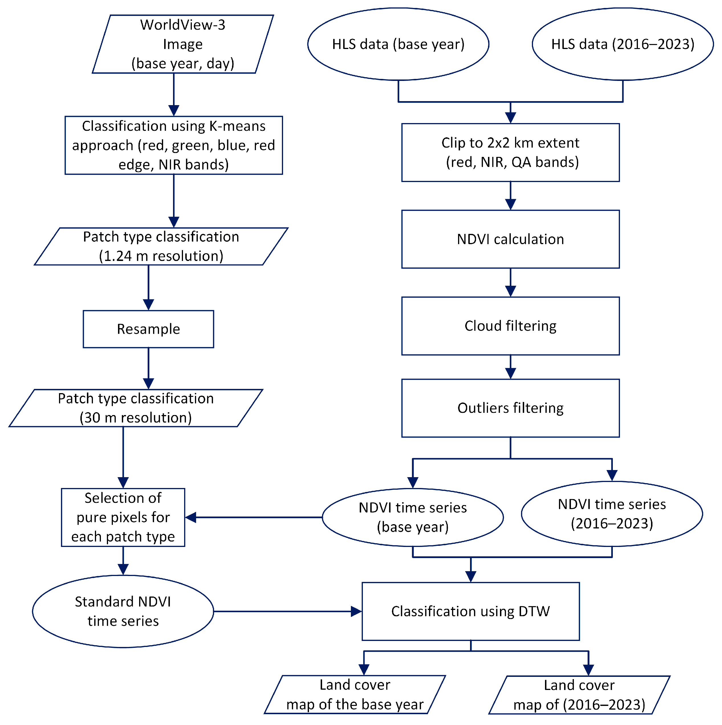
2.1. NDVI-Based Classification Overview

As a joint product of NASA/USGS Landsat 8 and ESA Sentinel-2A and Sentinel-2B satellites, NASA’s HLS provides surface reflectance data at a 30 m resolution for up to two to three days. Despite the limited spectral (7 bands) and spatial resolution of HLS compared to very-high-resolution multi-spectral products, such as WorldView, a seasonal timeseries of HLS-NDVI proved very effective at classifying patch-types within wetlands. A marked advantage of HLS is the short revisit time, which even after discarding cloud-obscured images, still resolves the seasonal temporal timeseries of NDVI for pixels within the wetland [18]. We followed the approach developed by Ju and Bohrer [10]. The approach is explained briefly in the sections below and illustrated in Figure 1. While the somewhat coarse HLS resolution leads to a high number of mixed pixels (given that wetland spatial heterogeneity could occur at a resolution of a few meters), it supports a high rate of correct classifications of the dominant patch-type [10]. Consequently, we can classify the patch structure within the wetland at the same spatial resolution as that of HLS, and during every season and year.

2.2. US-LA3 Wetland

NDVI-based classification and ELM simulations were implemented for a mesohaline marsh in the Barataria Basin of Louisiana. The site is a permanent wetland primarily covered by Juncus roemerianus and Spartina alterniflora, and with coordinates of (29.4936, −89.9153). The site’s terrain is flat with wind predominantly from the southeast. The site is a microtidal marsh that is flooded 16.88% of the time; it has an annual average salinity of 9.93 ppt, and 20–40% of its organic matter content is based on the Coastwide Reference Monitoring System database, station CRMS 0224 [19]. In addition, it is an Ameriflux site (Site ID US-LA3, [20]), where Eddy Covariance flux measurements are taken in addition to other ground-based measurements of aerenchyma conductance, chamber-based measurements of fluxes from specific patch-types. The site’s mean annual temperature is 20.9 degree Celsius and annual precipitation is 1623 mm [20]. The Eddy Covariance data include carbon fluxes and meteorological data (air temperature, relative humidity, pressure, wind speed and direction, net radiation, photosynthetic active radiation, soil temperature, and precipitation). The Gross Primary Production (GPP) and ecosystem respiration (ER) were modeled from the observed net ecosystem exchange of CO2 (NEE) and additional meteorological variables using an artificial neural network [21] and following standard Ameriflux data processing [22]. The GPP and ER were used for model parameterization. Water depth, vegetation cover fraction, and surface water depth data were retrieved from the Coastwide Reference Monitoring System database, station CRMS 0224 [19], and used as input for the ELM.

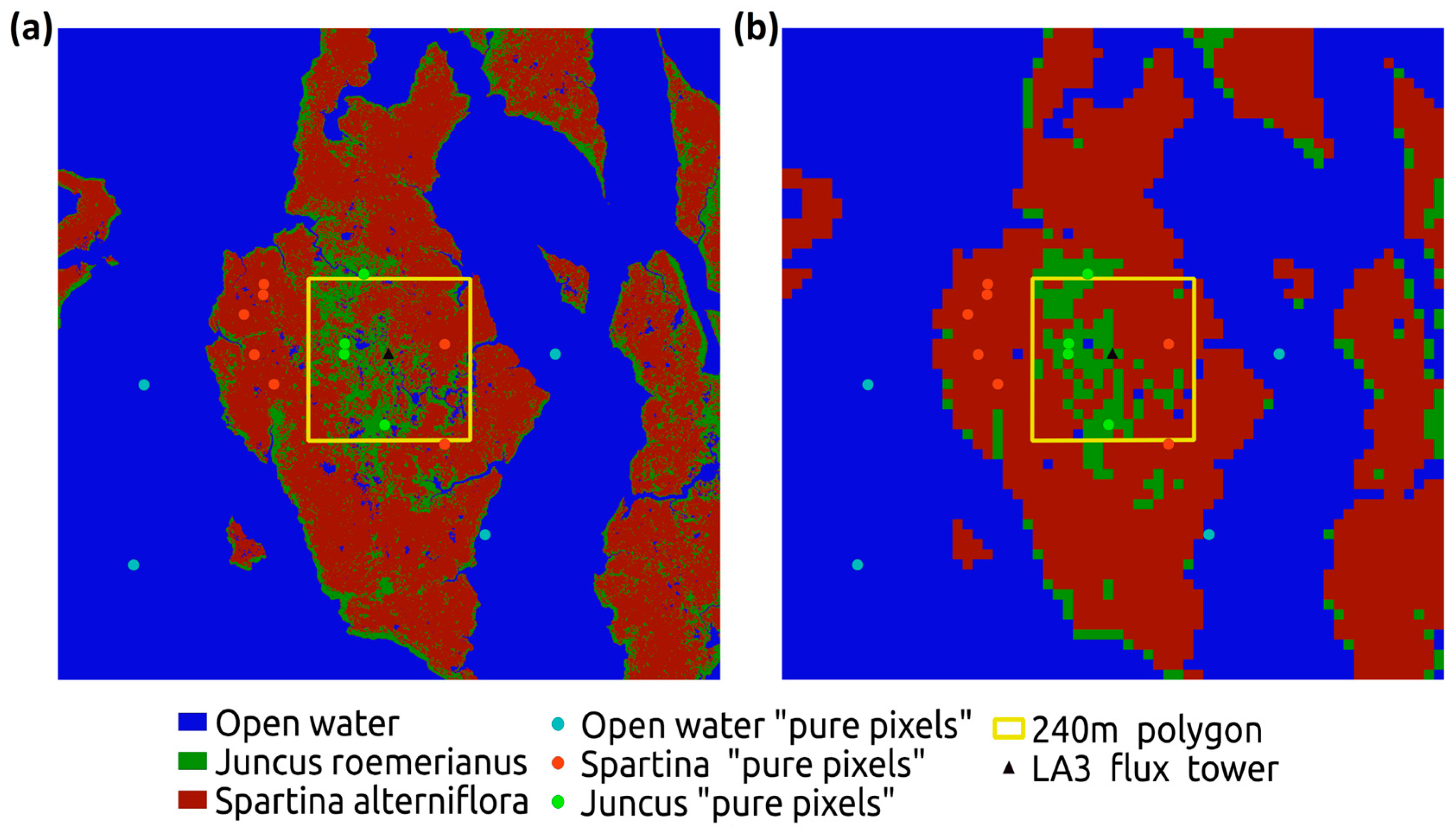
2.3. Classification of the Reference Patch-Types at the US-LA3 Site

Following Ju and Bohrer [10], we used a WorldView-3 multi-spectral image for day 18 August 2018 to develop a reference for the ground truth of the patch-type among the coarser HLS pixel locations. The WorldView-3 multi-spectral image was requested through the Commercial Smallsat Data Acquisition (CSDA) Program as Pansharpened (level 2A). The Image ID is 10400100408C8100. The image resolution was 1.24 m, and it fitted the quality-check requirements for most pixels included within the image, which overlap with the wetland area. The supervised classification of the high-resolution WorldView image during peak growing season was used as reference for the ground truth patch-type observation. We used reflectance data in several spectral bands at once to group pixels with similar values. Red, green, blue, and red edge and NIR bands were used as input data for cluster analysis, applying the K-means approach and using Euclidean distance as the metric. The image pixels were classified using a predetermined number of classes, which for US-LA3 were three: Juncus-dominated, Spartina-dominated, and open water (Figure 2a). This classified image was rasterized and upscaled to match the HLS resolution. Each HLS-matching pixel in this upscaled WorldView image was reclassified based of the dominant (>50%) type among all pixels of the original high-resolution WorldView image within that upscaled pixel. We identified 10 “pure pixels” of Spartina and 5 of Juncus (Juncus is much less present than Spartina). “Pure pixels” are defined such that at least 80% of the original WorldView high-resolution pixels within a single upscaled HLS-matching pixel belonged to the same patch-type (Figure 2b). Satellite data was processed using GDAL 3.6.4 and the corresponding calculations for the site classification were performed using Python 3.11 code relying on open-source packages. In particular, tslearn 0.6.3 package was applied for cluster analysis. Site classification was visualized using QGIS 3.22.

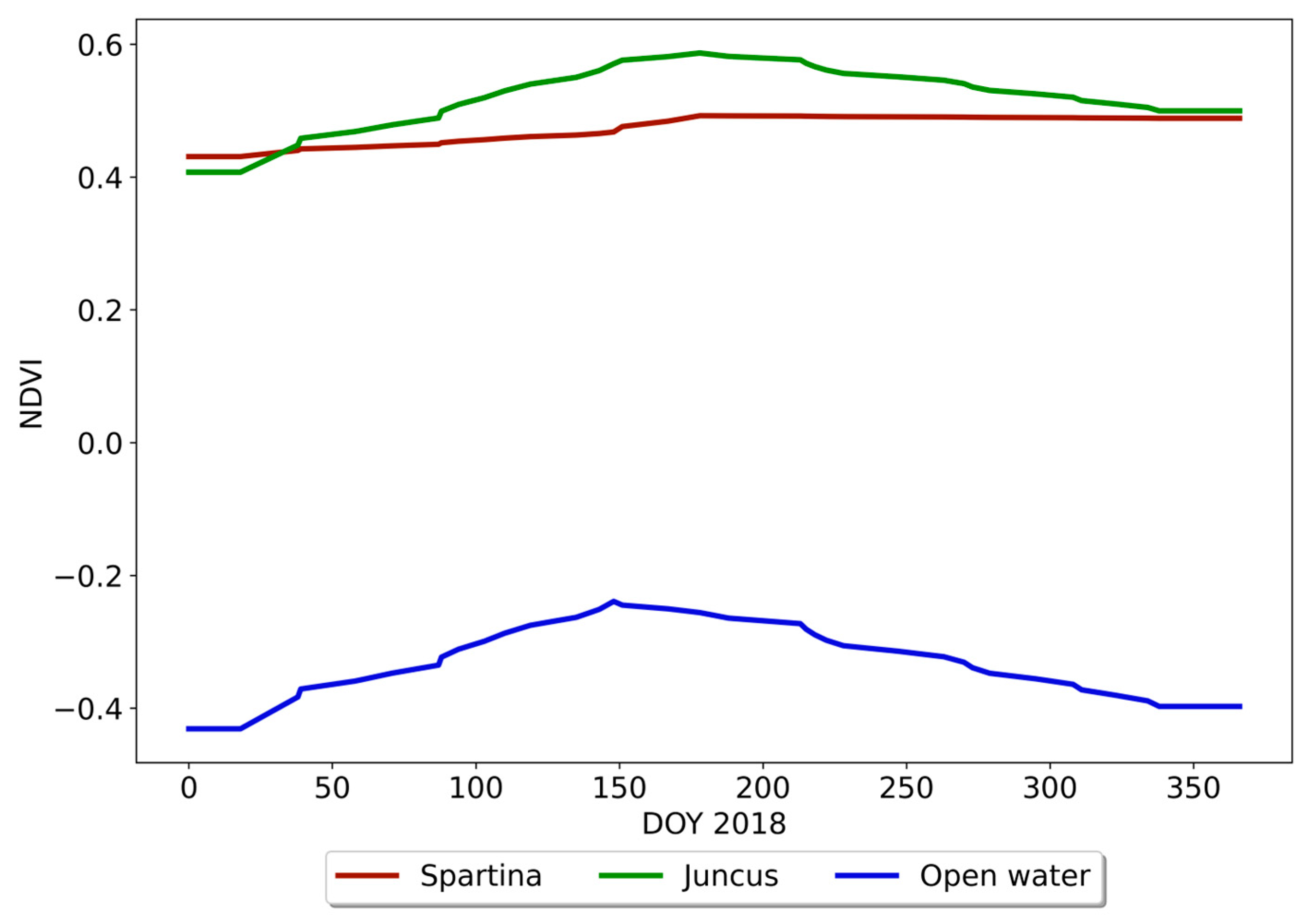
2.4. Seasonal NDVI Timeseries-Based Classification of Patch-Types at US-LA3 from HLS

We used HLS data containing two main surface reflectance products: (1) Setntinal-2A and Sentinel-2B and (2) Landsat (https://lpdaac.usgs.gov/products/hlsl30v002/ (accessed 1 August 2023) and https://lpdaac.usgs.gov/products/hlss30v002/ (accessed on 1 August 2023) for Landsat and Sentinel datasets, respectively). Our site falls within tile 16RBT. For each pixel, the Normalized Difference Vegetation Index was calculated using the HLS-retrieved red and NIR bands:
NDVI   = NIR     Red / NIR   +   Red
Using Equation (1), we calculated the NDVI index for each pixel of the HLS dataset and retrieved a timeseries for each year in the range of 2016–2023.
We matched each pixel locations in the HLS images during the growing season surrounding August 2018 to the corresponding pixels in the upscaled WorldView image. We further identified the locations selected as “pure pixels”. For each pure pixel, we extracted the seasonal timeseries of the NDVI during that growing season. We averaged these timeseries per patch-type (keeping all the temporal points within the season and averaging over all pure pixel locations of the same patch-type within each time frame). This average timeseries was defined as the characteristic NDVI seasonal “standard” per patch (Figure 3). We then used the Dynamic Time Warping (DTW) approach [23] to calculate the similarity between the seasonal timeseries of each of the other HLS pixels (including locations that were not selected as “pure” during the growing season of 2018, and all pixel locations in the HLS images of other years) and these characteristic seasonal standards. We identified the dominant patch-type as the type with the characteristic timeseries that is the most similar to the one observed in each pixel location, each year. The area of interest for ELM simulations is the vegetation cover within the fetch of the Eddy Covariance tower, which was ~250 m in our case. Thus, the area within the tower’s observation footprint can be roughly defined as a 480 m × 480 m square centered at the tower. This area was included in the patch-type classification used as an input for the ELM. This classification was conducted for each of the years of 2016–2023. Figure 3 shows the timeseries of HLS-classified patch-types for US-LA3.

2.5. ELM Overview and Simulation Set-Up

The ELM is a well-established land model that has been used in many studies [24,25,26,27,28,29,30,31], with some focusing on wetlands [4,32]. The ELM wetland methane module was derived from CLM4Me [2], wherein the model is capable of simulating methane production and oxidation, while also accounting for the three key pathways of methane transport: diffusion, ebullition, and plant aerenchyma. Recent developments targeting the wetland land unit in the ELM focused on representing the different vegetation types within a wetland at the sub-grid level. Such improvements helped represent the within-wetland biogeochemical and hydrological heterogeneity of eco-hydrological patches forming a wetland and improved the resulting methane flux and soil concentration estimations by reducing their corresponding uncertainties.
US-LA3 was simulated using an ELM. Simulations were spun-up according to protocols in [33]. Spin-up was divided into a 400-year-period of accelerated spin-up that allowed the accumulation of carbon to reach an equilibrium state, followed by a regular spin-up for another 400 years, when normal decomposition parameters were applied [27]. After spin-up, the model was run from year 1850 until 2023 using the Global Soil Wetness Project forcing and historical CO2 concentrations [24,34]. Carbon flux measurements are available on-site for years 2021–2022. These data were used to parameterize the model so that it was more representative of the site’s methane and CO2 dynamics. Parameterization included the parameters controlling photosynthesis and respiration. The objective function was set to minimize the root mean square error between modeled and observed EC flux timeseries, namely the Gross Primary Production (GPP) and ecosystem respiration (RECO). The Bayesian Optimization for Anything (BOA) workflow was used in the optimization process [35]. Observation-based vegetation-specific parameter values for the conductance of methane (in the soil and plant aerenchyma) and surface water elevation were prescribed as input and forcing for the model, respectively. ELM results processing was performed using Matlab 2018b.

2.6. Field Data

Many ground-based field measurements were used to parametrize the model. Flux data were derived from the US-LA3 Eddy Covariance tower measuring carbon fluxes in addition to meteorological variables (air temperature, relative humidity, pressure, wind speed and direction, net radiation, photosynthetic active radiation, soil temperature, and precipitation) for years 2021 and 2022. Surface water depth data (used as a forcing in the model) were retrieved from the Coastwide Reference Monitoring System database, station CRMS 0224 (CPRA 2023). Chamber flux and porewater samplings were conducted for methane flux and methane soil concentrations, respectively, over years 2021 and 2022 [36], which in return were used to calculated the vegetation-specific conductance for methane flux.

3. Results

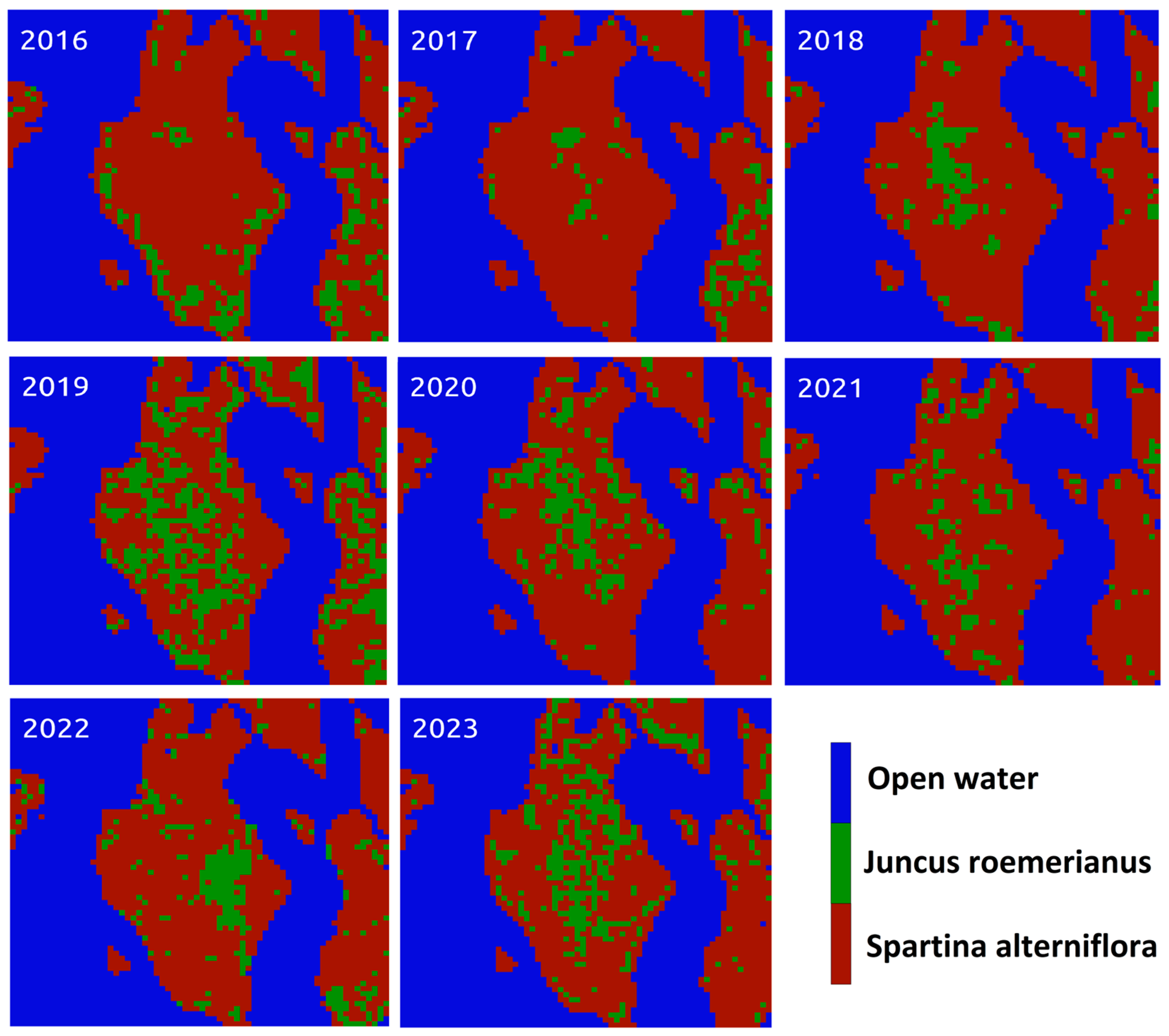
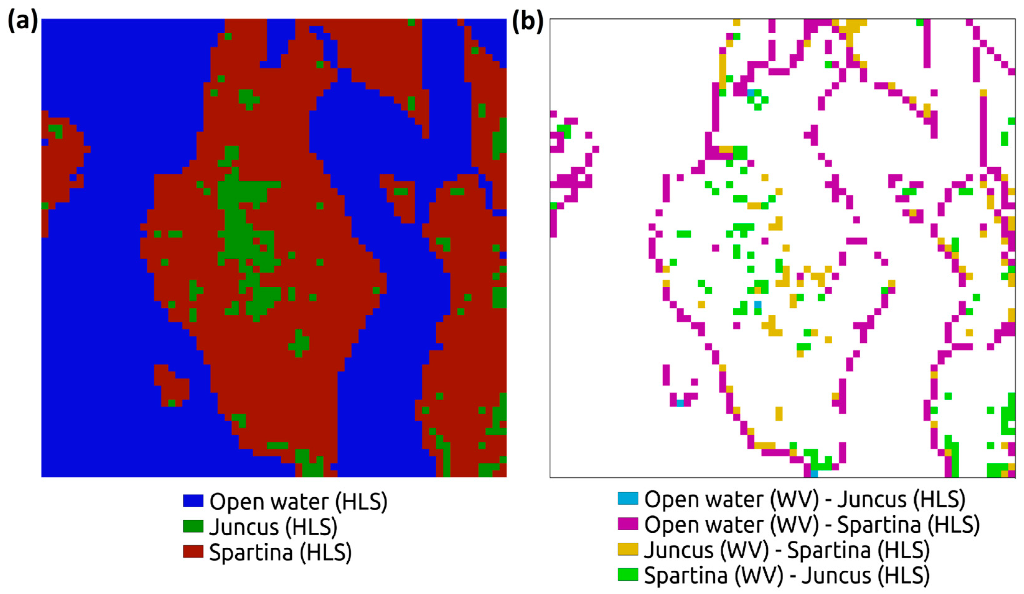
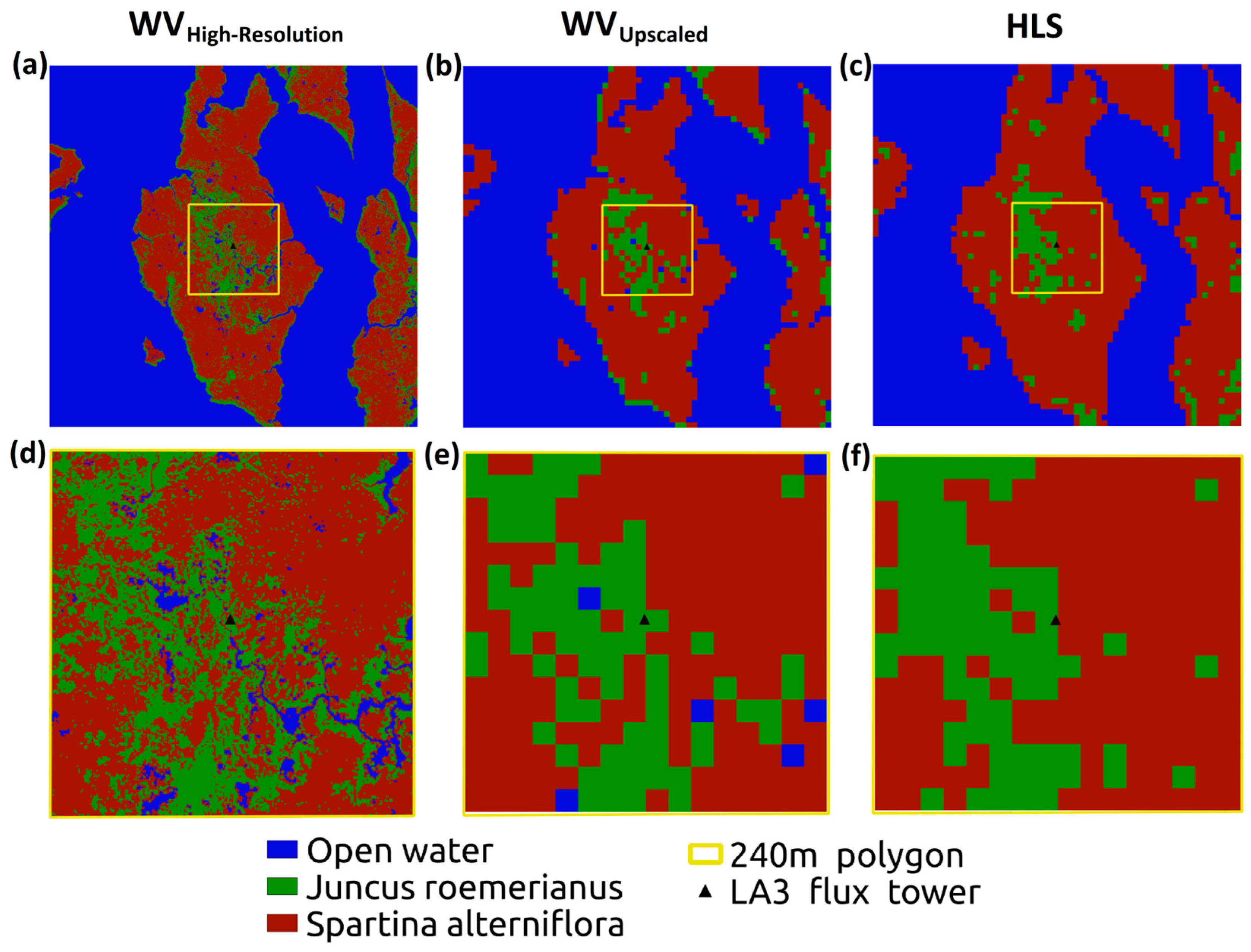
3.1. US-LA3 Classification
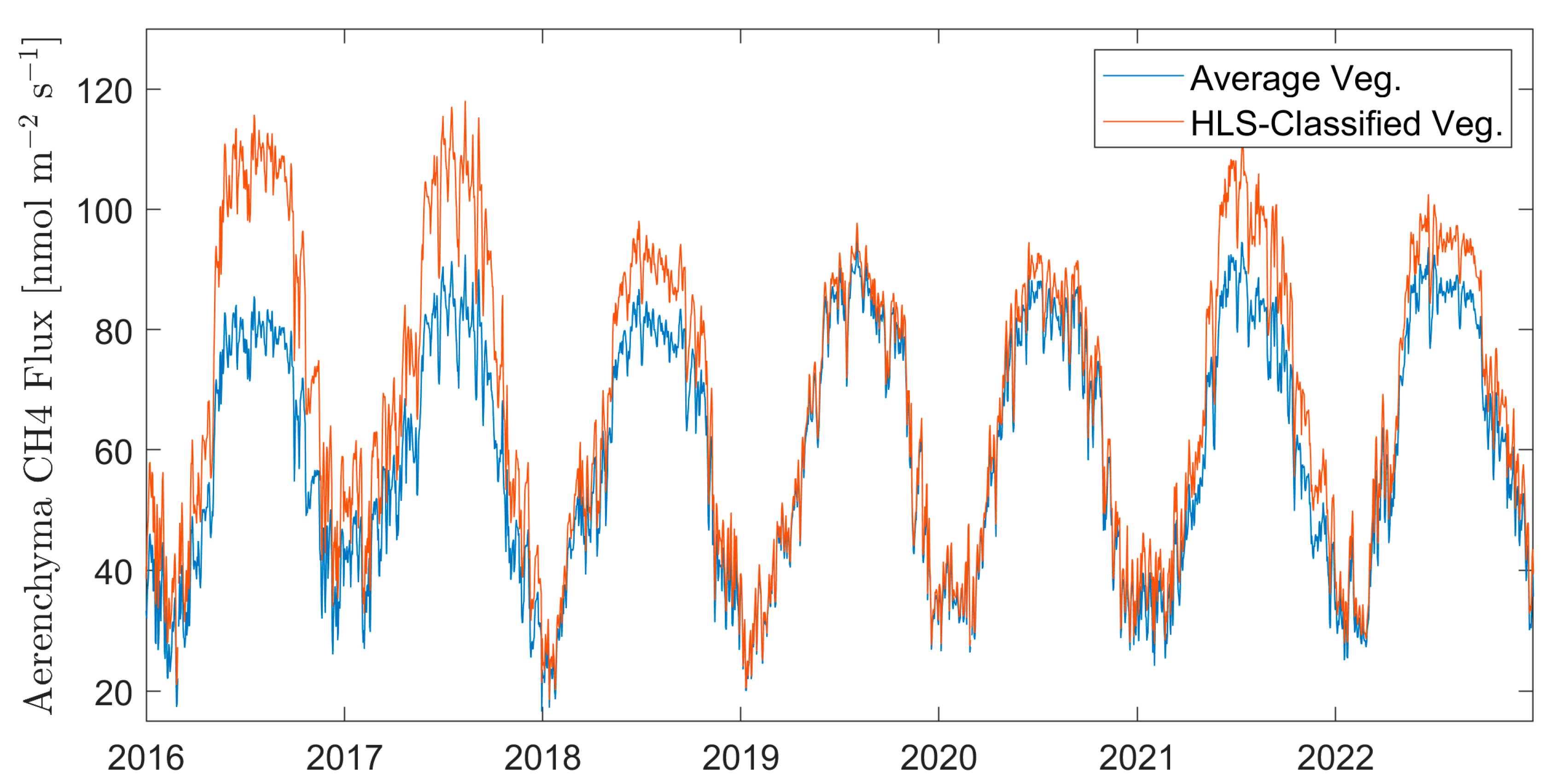
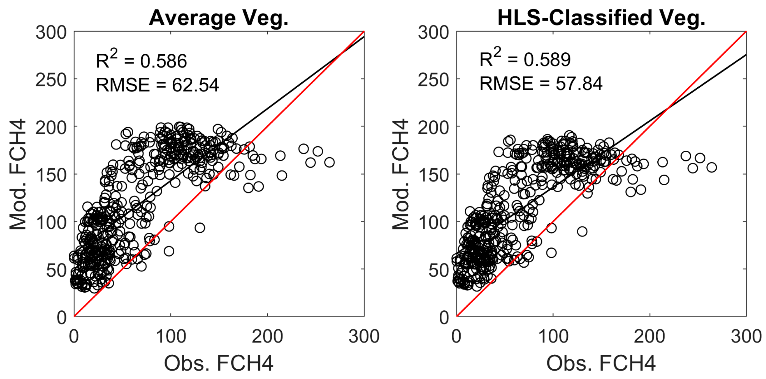
Since we considered the classification based on the WordView-3 data to be close to the truth based on the field observations, we evaluated the accuracy of the HLS classification through a confusion matrix of the WorldView-3 classification and the HLS classification results (Table 1). According to the HLS NDVI timeseries classification, open water and Spartina patches were recognized quite successfully (86.74% and 93.45%, respectively), while the Juncus classification had an accuracy of only 55.66%.
Using the NDVI-based method, the patch distribution for the years 2016 through 2023 were derived. Figure 4 shows the yearly classification for each of the three distinct patch-types in the wetland, and Table 2 summarizes the vegetation cover under the tower footprint based on the NDVI-based classification used as input for the ELM to derive the corresponding methane and carbon flux.

3.2. ELM Results

Two different sets of ELM simulations of US-LA3 were run from years 2016–2023. The first one used a constant vegetation coverage where the site was assumed to be 50% Spartina and 50% Juncus. The second one used the HLS-classification results listed in Table 2 to prescribe the yearly vegetation patch-type distribution. Our analysis focused on comparing the results from the two ELM simulations regarding aerenchyma flux (plant-mediated methane transport), which is one of the three components of total methane flux, and the most sensitive to vegetation type. Figure 5 shows that, when using HLS classification for vegetation cover to run the model, the aerenchyma flux shows high interannual variability, with high fluxes in years 2016–2017, followed by a significant decrease around years 2018–2021, and further followed by an increase in the following years.
In order to assess the impact of HLS data on the ELM’s methane estimations, we evaluated both simulations against the observed methane flux at the Eddy Covariance flux tower at US-LA3. The EC tower provides the data of the total methane flux over years 2021–2022 at a half-hourly timescale. As presented in Figure 6, model validation results (using a linear regression between the observed and modeled total methane flux) showed a slight improvement in R2, while a more significant improvement is observed in the Root Mean Square Error (RMSE) of the regression, which was decreased by 7.5% when using HLS-classified vegetation cover.

4. Discussion

The confusion matrix results show that Spartina-dominated patches were better classified than Juncus-dominated ones, where the base-year HLS classification for Spartina had a 93.45% match with the WorldView classification compared to 55.66% for Juncus, which was often misclassified as Spartina. This is largely due to the fact that both species’ NDVI timeseries are close in terms of absolute values, with a difference in that Juncus shows a distinct NDVI peak in July, i.e., an increase in the early growing season, that is then followed by a browning period at the end of the season, while Spartina is more constant over the year (Figure 3). The site is dominated by Spartina, where Juncus patches are dispersed within Spartina-dominated areas. As shown in Figure 7b, most of the misclassified pixels for both Juncus and Spartina are present in the middle of the wetland (away from water edges). We suspect that these pixels present a true near-equal mix of both vegetations, which led to this apparent misclassification. The abundance of these misclassified pixels (yellow and green pixels in Figure 7b) is similar for both vegetation types in that central area, but since Juncus is much less abundant than Spartina, they represent a large portion of the Juncus, leading to the high percentage of misclassified Juncus pixels. As for misclassified open water pixels, most were misclassified as Spartina and were mostly present at the vegetation–water edge (Figure 7b).
Our results correspond with those of several studies that made use of reflectance data to obtain NDVIs and use them as a tool for land cover classification [37,38], with a special focus on vegetation classification in inundated areas [39,40]. Ouyang et al. [41] showed that the differences in saltmarsh communities’ spectral characteristics is a function of their phenological stages, while Gao et al. [42] has showed that spectral characteristics across seasons improve saltmarsh vegetation classification. Thus, the inclusion of NDVI timeseries instead of relying on NDVI point measurements plays an important role in improving wetland mapping [43]. A similar approach to our NDVI-based classification of within-wetland vegetation type was presented by Sun et al. [44], where the HuanJing 1 (HJ-1) satellite was used to build monthly NDVI timeseries and classify saltmarshes in the coast of Jiangsu in east China, which resulted in accurate classifications of vegetation types, thus emphasizing the promising role that NDVI timeseries has in classifying within-wetland eco-hydrological patches [45].
Including the classification results as input in the ELM simulations led to substantial improvements in the plant-mediated methane flux, known as aerenchyma (Figure 5), whereby in including the yearly vegetation classification, the methane flux was then a function of the vegetation cover and the impact of the latter is shown in the ELM-output methane flux. Spartina is more conductive to methane flux compared to Juncus [36]; thus, whenever more Juncus is present on-site, a lesser total of aerenchyma flux should be emitted from the site. Note that this does not necessarily mean that more total methane flux would be emitted. Indeed, as shown in Figure 5, the increase in the Juncus presence over years 2018 and 2019 was reflected in a reduced aerenchyma flux when using HLS-derived classification, which was not the case when using a constant average vegetation cover over all simulated years.
The validation results using methane flux observations show that using HLS-derived classification reduced the estimation error of the predicted total methane flux by around 7.5%. It must be noted that the EC tower measures the total flux, which includes contributions from the three methane transport pathways: diffusion, ebullition, and aerenchyma. Using the HLS-derived classification is expected to particularly improve the representation of the dynamics of methane aerenchyma transport. In our version of an ELM, we resolved each vegetation as a separate soil column, where minimal feedback existed between the two simulated vegetation types. Therefore, the effect that HLS-derived classification had on the total methane flux was mostly through correctly weighting the methane transport dynamics (mostly ebullition and aerenchyma) between the different vegetations when deriving the total methane flux.

HLS-Classification Uncertainty and Its on Impact Simulated Methane Flux

There is a significant gap between the small scale of vegetation heterogeneity (scale of a few 10s of cm) and the HLS resolution (30 m × 30 m). Therefore, HLS NDVI-based classification will assign each pixel to the majority of its vegetation cover, thus over-representing the dominant patch-type and under-representing less common types that do not form large patches, which could provide a source of bias in the classification results. In addition, another source of uncertainty is attributed to the increased cloud presence during the early growing season. A main component of the NDVI-based classification method is the NDVI timeseries derived from the “pure pixels” used as a standard to classify all other pixels to their dominant patch-type. It is common to have missing NDVI observations in the early growing season due to increased cloud cover, which coincides with the increase in the vegetation NDVI, defining the trend or signature of this specific patch-type compared to others. These high-cloud-cover data points are usually filtered out during data processing, which would contribute to the uncertainty coupled with the NDVI-based classification.
In order to further analyze the uncertainty introduced with the use of the HLS-derived classification method, we compared its results to those of the WorldView-derived classification for year 2018 within our area of interest, i.e., 480 × 480 m2 around the EC tower. Using the supervised classification of the WV data, we obtained the high-resolution (1.24 m), high-accuracy classification (WVHigh-Resolution). Then, we upscaled the WV high-resolution grid to the HLS resolution (30 m × 30 m) and counted the majority patch-type in each upscaled pixel to obtain a WVUpscaled classification, matching the HLS resolution, but accounting for high-accuracy data. We compared these two classification results to those of the HLS-derived classification. Table 3 shows the results of the classification of each method and the difference (Δ) or mismatch between the three different methods. Figure 8 shows the corresponding classification map of the three techniques. The results show that upscaling to the HLS resolution leads to an underestimation of open water patches in the area of interest (where open water patches are rare and small), but with a minimal effect on the final overall results (Table 3).
In order to further investigate this impact on the total methane flux, we ran the ELM for 2018 using the WVHigh-Resolution classification results and obtained the RMSE between simulated methane flux using WVHigh-Resolution as input for the vegetation cover and simulated methane flux using HLS as input for vegetation cover. The RMSE between these two simulations is 3.14 nmol m−2 s−1, which we consider to be the error introduced to the total methane flux using the HLS-derived classification method. To have a better understanding of the uncertainty introduced by the HLS method, we compare it to the estimated error of the EC flux measurement, which in our case was 27 nmol m−2 s−1 at US-LA3 for the two years when measurements were available (2021–2022). Thus, the error introduced to the methane flux simulation results due to the HLS classification error is minimal, especially when compared to the existing uncertainty of methane flux observations.
Although NDVI-based classification using HLS data showed to be a good estimate of yearly vegetation cover at the wetland site and improved the estimation of methane flux, there are gaps that need to be addressed in order to further reduce the uncertainty in methane flux estimations. Our NDVI-based classification provides information about the vegetation cover map without accounting for the inundation dynamics at the site. We effectively assumed that the vegetation cover in a given pixel remains the same for the whole year, and that there are no other sources of environmental variability among patches of the same type (e.g., all open-water patches have the same depth). However, these vegetation covers are changing from a diurnal/weekly level due to daily changes in surface water elevation to other slower effects such as saline intrusion and herbivory, which should to be taken into consideration for more accurate estimations of the effects of vegetation cover on surface fluxes [46]. Although our version of the ELM uses observed water surface elevations to force the water dynamics of the wetland, we did not include high-resolution bathymetry information, which could help define the dynamics of intra-annual vegetation cover, and account for additional spatial heterogeneity. In addition, it must be noted that methane estimations in LSMs are subject to many sources of error other than those related to the accurate representation of the within-wetland eco-hydrological patch-types. These limitations include the bulk representation of methane production in LSMs, which is usually set to be a function of upland biogeochemistry while not representing the different pathways for methane production [47,48]. In addition, the lack of representation of lateral flow between grid-cells, which limits the ability of LSMs in resolving reactive transport, which in turn will result in biases with modeling methane oxidation and inundation dynamics. Many efforts are underway to overcome these limitations and have a better representation of methane dynamics in wetlands [49], and improved patch-type observations will serve these efforts well.

5. Conclusions

In this study, we implemented a within-wetland eco-hydrological patch classification using the NDVI-based technique using NASA’s Harmonized Landsat-Sentinel open-source dataset. The classification was applied on a coastal wetland in Louisiana, a brackish marsh dominated by intermittent Juncus and Spartina vegetation with sparse open water patches. The classification results were then used as input for the E3SM Land Model to provide the model with necessary information about the wetland’s vegetation cover over the simulated years and used to improve methane flux estimations from the site. Classification showed very good results for Spartina and open water that were mostly, successfully classified, while Juncus had a lower performance due to the close range of the NDVI compared to that of Spartina. The ELM simulations showed that accounting for the observed vegetation cover change over the years improved the representation of methane flux dynamics, while reducing the uncertainty of the total methane flux estimations. The error introduced by resampling WorldView data to the HLS resolution showed to have minimal effect on the classification and, consequently, the methane flux results. The NDVI-based classification approach offers a substitute for ground observations of vegetation patch-type distribution in wetlands worldwide. Using the processed remote sensing observations of vegetation patch-types will allow us to account for vegetation distribution impacts on the plant-mediated methane flux from wetlands, usually responsible for the significant methane emissions from coastal wetlands. Our study shows promising results for integrating the remote sensing-based mapping of land cover change into land surface models, which would significantly improve their performance and lead to more accurate predictions.

Author Contributions

This manuscript was written and prepared by T.Y. and O.S. under the supervision of G.B. The NDVI-based classification was originally conceived by Y.J. and G.B.; E.W., R.B. and J.A.V. contributed to the field data measurements and the validating of the results of US-LA3. All authors have read and agreed to the published version of the manuscript.

Funding

This research was funded in part by the U.S. Department of Energy awards DE-SC0023084 and DE-SC0021067 and NASA FINNEST Fellowship 80NSSC22K1527. Funding for eddy covariance data collection was provided by the USGS South Central Climate Adaptation Science Center, USGS LandCarbon Program and USGS Ecosystems Mission Area. Apache Louisiana Minerals provided access to the site of this study.

Data Availability Statement

HLS data can be found at https://lpdaac.usgs.gov/products/hlsl30v002/ (accessed on 1 August 2023) and https://lpdaac.usgs.gov/products/hlss30v002/ (accessed on 1 August 2023), for the Landsat and Sentinel datasets, respectively. Our site falls within tile 16RBT. The WorldView-3 multi-spectral image was requested through the Commercial SmallSat Data Acquisition (CSDA) Program as Pansharpened (level 2A). The Image ID is 10400100408C8100. The link to the CSDA program is as follows: https://www.earthdata.nasa.gov/esds/csda (accessed on 1 August 2023). The ELM version used in this study can be found at the following github repository: https://github.com/theresiayazbeck/ELM_WetlandLandunit_Perlmutter (accessed on 1 August 2023). US-LA3 flux and meteorological data can be found on the Ameriflux website: https://ameriflux.lbl.gov/sites/siteinfo/US-LA3 (accessed on 1 August 2023). Methane conductance and soil concentration can be found on the ESS dive database: https://data.ess-dive.lbl.gov/view/doi:10.15485/1997524 (accessed on 1 August 2023). Surface water depth data at US-LA3 can be found at the CRIMS database: https://lacoast.gov/crms/ (accessed on 1 August 2023). The BOA model is open source and can be found at https://doi.org/10.5281/zenodo.8253924.

Acknowledgments

We would like to thank the National Energy Research Scientific Computing Center (NERSC) where we ran the ELM simulations. Runs were performed on the Perlmutter cluster. We would like to thank William J. Riley and Qing Zhu from Lawrence Berkeley National Laboratory for their continuous support and insights in developing the wetland land-unit in ELM. We would like to thank Sergio Merino from the USGS Wetland and Aquatic Research Center for their continuous support with providing the required information about field measurements at US-LA3.

Conflicts of Interest

The funders had no role in the design of the study; in the collection, analyses, or interpretation of data; in the writing of the manuscript; or in the decision to publish the results.

References

  1. Forster, P.; Storelvmo, T.; Armour, K.; Collins, W.; Dufresne, J.-L.; Frame, D.; Lunt, D.J.; Mauritsen, T.; Palmer, M.D.; Watanabe, M.; et al. The Earth’s Energy Budget, Climate Feedbacks, and Climate Sensitivity. In Climate Change 2021: The Physical Science Basis. Contribution of Working Group I to the Sixth Assessment Report of the Intergovernmental Panel on Climate Change; Cambridge University Press: Cambridge, UK; New York, NY, USA, 2021; pp. 923–1054. ISBN 9781009157896. [Google Scholar]
  2. Riley, W.J.; Subin, Z.M.; Lawrence, D.M.; Swenson, S.C.; Torn, M.S.; Meng, L.; Mahowald, N.M.; Hess, P. Barriers to Predicting Changes in Global Terrestrial Methane Fluxes: Analyses Using CLM4Me, a Methane Biogeochemistry Model Integrated in CESM. Biogeosciences 2011, 8, 1925–1953. [Google Scholar] [CrossRef]
  3. Saunois, M.; Stavert, A.R.; Poulter, B.; Bousquet, P.; Canadell, J.G.; Jackson, R.B.; Raymond, P.A.; Dlugokencky, E.J.; Houweling, S.; Patra, P.K.; et al. The Global Methane Budget 2000–2017. Earth Syst. Sci. Data 2020, 12, 1561–1623. [Google Scholar] [CrossRef]
  4. Saunois, M.; Bousquet, P.; Poulter, B.; Peregon, A.; Ciais, P.; Canadell, J.G.; Dlugokencky, E.J.; Etiope, G.; Bastviken, D.; Houweling, S.; et al. Variability and Quasi-Decadal Changes in the Methane Budget over the Period 2000-2012. Atmos. Chem. Phys. 2017, 17, 11135–11161. [Google Scholar] [CrossRef]
  5. Villa, J.A.; Ju, Y.; Yazbeck, T.; Waldo, S.; Wrighton, K.C.; Bohrer, G. Ebullition Dominates Methane Fluxes from the Water Surface across Different Ecohydrological Patches in a Temperate Freshwater Marsh at the End of the Growing Season. Sci. Total Environ. 2021, 767, 144498. [Google Scholar] [CrossRef]
  6. Ge, M.; Korrensalo, A.; Laiho, R.; Lohila, A.; Makiranta, P.; Pihlatie, M.; Tuittila, E.-S.; Kohl, L.; Putkinen, A.; Koskinen, M. Plant Phenology and Species-Specific Traits Control Plant CH4 Emissions in a Northern Boreal Fen. New Phytol. 2023, 238, 1019–1032. [Google Scholar] [CrossRef] [PubMed]
  7. Jeffrey, L.C.; Maher, D.T.; Johnston, S.G.; Kelaher, B.P.; Steven, A.; Tait, D.R. Wetland Methane Emissions Dominated by Plant-Mediated Fluxes: Contrasting Emissions Pathways and Seasons within a Shallow Freshwater Subtropical Wetland. Limnol. Oceanogr. 2019, 64, 1895–1912. [Google Scholar] [CrossRef]
  8. Flato, G.M. Earth System Models: An Overview. Wiley Interdiscip. Rev. Clim. Chang. 2011, 2, 783–800. [Google Scholar] [CrossRef]
  9. LaFond-Hudson, S.; Sulman, B. Modeling Strategies and Data Needs for Representing Coastal Wetland Vegetation in Land Surface Models. New Phytol. 2023, 238, 938–951. [Google Scholar] [CrossRef]
  10. Ju, Y.; Bohrer, G. Classification of Wetland Vegetation Based on NDVI Timeseries from HLS Dataset. Remote Sens. 2022, 14, 2107. [Google Scholar] [CrossRef]
  11. Adam, E.; Mutanga, O.; Rugege, D. Multispectral and Hyperspectral Remote Sensing for Identification and Mapping of Wetland Vegetation: A Review. Wetl. Ecol. Manag. 2010, 18, 281–296. [Google Scholar] [CrossRef]
  12. Liao, T.H.; Simard, M.; Denbina, M.; Lamb, M.P. Monitoring Water Level Change and Seasonal Vegetation Change in the Coastal Wetlands of Louisiana Using L-Band Time-Series. Remote Sens. 2020, 12, 2351. [Google Scholar] [CrossRef]
  13. Bansal, S.; Katyal, D.; Saluja, R.; Chakraborty, M.; Garg, J.K. Remotely Sensed MODIS Wetland Components for Assessing the Variability of Methane Emissions in Indian Tropical/subtropical Wetlands. Int. J. Appl. Earth Obs. Geoinf. 2018, 64, 156–170. [Google Scholar] [CrossRef]
  14. Mousavi, S.M.; Falahatkar, S. Spatiotemporal Distribution Patterns of Atmospheric Methane Using GOSAT Data in Iran. Environ. Dev. Sustain. 2020, 22, 4191–4207. [Google Scholar] [CrossRef]
  15. Javadinejad, S.; Eslamian, S.; Ostad-Ali-Askari, K. Investigation of Monthly and Seasonal Changes of Methane Gas with Respect to Climate Change Using Satellite Data. Appl. Water Sci. 2019, 9, 180. [Google Scholar] [CrossRef]
  16. EarthData Harmonized Landsat Sentinel-2 (HLS). Available online: https://earthdata.nasa.gov/esds/harmonized-landsat-sentinel-2 (accessed on 1 June 2022).
  17. Claverie, M.; Ju, J.; Masek, J.G.; Dungan, J.L.; Vermote, E.F.; Roger, J.C.; Skakun, S.V.; Justice, C. The Harmonized Landsat and Sentinel-2 Surface Reflectance Data Set. Remote Sens. Environ. 2018, 219, 145–161. [Google Scholar] [CrossRef]
  18. Guo, M.; Li, J.; Sheng, C.; Xu, J.; Wu, L. A Review of Wetland Remote Sensing. Sensors 2017, 17, 777. [Google Scholar] [CrossRef]
  19. CPRA Coastwide Reference Monitoring System-Wetlands Monitoring Data. Available online: http://cims.coastal.louisiana.gov (accessed on 1 August 2023).
  20. Ward, E.; Merino, S.; Stagg, C.; Krauss, K. AmeriFlux BASE US-LA3 Barataria Bay Saline Marsh, Ver. 1-5, AmeriFlux AMP, (Dataset). 2023. Available online: https://ameriflux.lbl.gov/doi/AmeriFlux/US-LA3/ (accessed on 1 November 2023).
  21. Moffat, A.M.; Papale, D.; Reichstein, M.; Hollinger, D.Y.; Richardson, A.D.; Barr, A.G.; Beckstein, C.; Braswell, B.H.; Churkina, G.; Desai, A.R.; et al. Comprehensive Comparison of Gap-Filling Techniques for Eddy Covariance Net Carbon Fluxes. Agric. For. Meteorol. 2007, 147, 209–232. [Google Scholar] [CrossRef]
  22. Pastorello, G.; Trotta, C.; Canfora, E.; Chu, H.; Christianson, D.; Cheah, Y.W.; Poindexter, C.; Chen, J.; Elbashandy, A.; Humphrey, M.; et al. The FLUXNET2015 Dataset and the ONEFlux Processing Pipeline for Eddy Covariance Data. Sci. Data 2020, 7, 225. [Google Scholar] [CrossRef] [PubMed]
  23. Sakoe, H.; Chiba, S. Dynamic Programming Algorithm Optimization for Spoken Word Recognition. IEEE Trans. Acoust. 1978, 26, 43–49. [Google Scholar] [CrossRef]
  24. Zhu, Q.; Riley, W.J.; Tang, J.; Collier, N.; Hoffman, F.M.; Yang, X.; Bisht, G. Representing Nitrogen, Phosphorus, and Carbon Interactions in the E3SM Land Model: Development and Global Benchmarking. J. Adv. Model. Earth Syst. 2019, 11, 2238–2258. [Google Scholar] [CrossRef]
  25. Riley, W.J.; Zhu, Q.; Tang, J.Y. Weaker Land–climate Feedbacks from Nutrient Uptake during Photosynthesis-Inactive Periods. Nat. Clim. Chang. 2018, 8, 1002–1006. [Google Scholar] [CrossRef]
  26. Tang, J.; Riley, W.J. Predicted Land Carbon Dynamics Are Strongly Dependent on the Numerical Coupling of Nitrogen Mobilizing and Immobilizing Processes: A Demonstration with the E3SM Land Model. Earth Interact. 2018, 22, 1–18. [Google Scholar] [CrossRef]
  27. Yuan, F.; Wang, Y.; Ricciuto, D.M.; Shi, X.; Yuan, F.; Hanson, P.J.; Bridgham, S.; Keller, J.; Thornton, P.E.; Xu, X. An Integrative Model for Soil Biogeochemistry and Methane Processes. II: Warming and Elevated CO2 Effects on Peatland CH4 Emissions. J. Geophys. Res. Biogeosciences 2021, 126, e2020JG005963. [Google Scholar] [CrossRef]
  28. Li, L.; Bisht, G.; Leung, L.R. Spatial Heterogeneity Effects on Land Surface Modeling of Water and Energy Partitioning. Geosci. Model Dev. 2022, 15, 5489–5510. [Google Scholar] [CrossRef]
  29. Hao, D.; Bisht, G.; Rittger, K.; Bair, E.; He, C.; Huang, H.; Dang, C.; Stillinger, T.; Gu, Y.; Hailong, W.; et al. Improving Snow Albedo Modeling in the E3SM Land Model (Version 2.0) and Assessing Its Impacts on Snow and Surface Fluxes over the Tibetan Plateau. Geosci. Model Dev. 2023, 16, 75–94. [Google Scholar] [CrossRef]
  30. Hao, D.; Bisht, G.; Gu, Y.; Lee, W.L.; Liou, K.N.; Leung, L.R. A Parameterization of Sub-Grid Topographical Effects on Solar Radiation in the E3SM Land Model (Version 1.0): Implementation and Evaluation over the Tibetan Plateau. Geosci. Model Dev. 2021, 14, 6273–6289. [Google Scholar] [CrossRef]
  31. Burrows, S.M.; Maltrud, M.; Yang, X.; Zhu, Q.; Jeffery, N.; Shi, X.; Ricciuto, D.; Wang, S.; Bisht, G.; Tang, J.; et al. The DOE E3SM v1.1 Biogeochemistry Configuration: Description and Simulated Ecosystem-Climate Responses to Historical Changes in Forcing. J. Adv. Model. Earth Syst. 2020, 12, e2019MS001766. [Google Scholar] [CrossRef]
  32. Poulter, B.; Bousquet, P.; Canadell, J.G.; Ciais, P.; Peregon, A.; Saunois, M.; Arora, V.K.; Beerling, D.J.; Brovkin, V.; Jones, C.D.; et al. Global Wetland Contribution to 2000–2012 Atmospheric Methane Growth Rate Dynamics OPEN ACCESS Global Wetland Contribution to 2000–2012 Atmospheric Methane Growth Rate Dynamics. Environ. Res. Lett. 2017, 12, 094013. [Google Scholar] [CrossRef]
  33. Oleson, K.W.; Lawrence, D.M.; Bonan, G.B.; Drewniak, B.; Huang, M.; Charles, D.; Levis, S.; Li, F.; Riley, W.J.; Subin, Z.M.; et al. CLM 4.5 NCAR Technical Note. In Technical Description of Version 4.5 of the Community Land Model (CLM); National Center for Atmospheric Research: Boulder, CO, USA, 2013. [Google Scholar] [CrossRef]
  34. Dirmeyer, P.A.; Gao, X.; Zhao, M.; Guo, Z.; Oki, T.; Hanasaki, N. GSWP-2: Multimodel Analysis and Implications for Our Perception of the Land Surface. Bull. Am. Meteorol. Soc. 2006, 87, 1381–1397. [Google Scholar] [CrossRef]
  35. Scyphers, M.; Missik, J.; Paulson, J.; Bohrer, G. Bayesian Optimization for Anything (BOA) (0.10.2). Zenodo. 2023. Available online: https://zenodo.org/records/10067681 (accessed on 1 November 2023).
  36. Bordelon, R.; Villa, J.; Taj, D.; Moore, M.; Mina, J.; Merino, S.; Ward, E.; Bohrer, G. CO2 and CH4 Leaf-Level Fluxes and Soil Porewater Concentrations from Common Vegetation Patches in Louisiana’s Coastal Wetlands. Functional-Type Modeling Approach and Data-Driven Parameterization of Methane Emissions in Wetlands. Available online: https://data.ess-dive.lbl.gov/datasets/doi:10.15485/1997524 (accessed on 1 November 2023).
  37. Kayastha, N.; Thomas, V.; Galbraith, J.; Banskota, A. Monitoring Wetland Change Using Inter-Annual Landsat Time-Series Data. Wetlands 2012, 32, 1149–1162. [Google Scholar] [CrossRef]
  38. Arastoo, B.; Ghazaryan, S.; Avetyan, N. An Approach for Land Cover Classification System by Using NDVI Data in Arid and Semiarid Region. Elixir Remote Sens. 2013, 60, 16327–16332. [Google Scholar]
  39. Lane, C.R.; Liu, H.; Autrey, B.C.; Anenkhonov, O.A.; Chepinoga, V.V.; Wu, Q. Improved Wetland Classification Using Eight-Band High Resolution Satellite Imagery and a Hybrid Approach. Remote Sens. 2014, 6, 12187–12216. [Google Scholar] [CrossRef]
  40. Fernandes, M.R.; Aguiar, F.C.; Silva, J.M.N.; Ferreira, M.T.; Pereira, J.M.C. Spectral Discrimination of Giant Reed (Arundo donax L.): A Seasonal Study in Riparian Areas. ISPRS J. Photogramm. Remote Sens. 2013, 80, 80–90. [Google Scholar] [CrossRef]
  41. Ouyang, Z.T.; Gao, Y.; Xie, X.; Guo, H.Q.; Zhang, T.T.; Zhao, B. Spectral Discrimination of the Invasive Plant Spartina Alterniflora at Multiple Phenological Stages in a Saltmarsh Wetland. PLoS ONE 2013, 8, e67315. [Google Scholar] [CrossRef] [PubMed]
  42. Gao, Z.G.; Zhang, L.Q. Multi-Seasonal Spectral Characteristics Analysis of Coastal Salt Marsh Vegetation in Shanghai, China. Estuar. Coast. Shelf Sci. 2006, 69, 217–224. [Google Scholar] [CrossRef]
  43. Xu, P.; Niu, Z.; Tang, P. Comparison and Assessment of NDVI Timeseries for Seasonal Wetland Classification. Int. J. Digit. Earth 2018, 11, 1103–1131. [Google Scholar] [CrossRef]
  44. Sun, C.; Liu, Y.; Zhao, S.; Zhou, M.; Yang, Y.; Li, F. Classification Mapping and Species Identification of Salt Marshes Based on a Short-Time Interval NDVI Time-Series from HJ-1 Optical Imagery. Int. J. Appl. Earth Obs. Geoinf. 2016, 45, 27–41. [Google Scholar] [CrossRef]
  45. Li, H.; Wan, J.; Liu, S.; Sheng, H.; Xu, M. Wetland Vegetation Classification through Multi-Dimensional Feature Timeseries Remote Sensing Images Using Mahalanobis Distance-Based Dynamic Time Warping. Remote Sens. 2022, 14, 501. [Google Scholar] [CrossRef]
  46. Chen, L.; Jin, Z.; Michishita, R.; Cai, J.; Yue, T.; Chen, B.; Xu, B. Dynamic Monitoring of Wetland Cover Changes Using Time-Series Remote Sensing Imagery. Ecol. Inform. 2014, 24, 17–26. [Google Scholar] [CrossRef]
  47. Melton, J.R.; Wania, R.; Hodson, E.L.; Poulter, B.; Ringeval, B.; Spahni, R.; Bohn, T.; Avis, C.A.; Beerling, D.J.; Chen, G.; et al. Present State of Global Wetland Extent and Wetland Methane Modelling: Conclusions from a Model Inter-Comparison Project (WETCHIMP). Biogeosciences 2013, 10, 753–788. [Google Scholar] [CrossRef]
  48. Xu, X.; Yuan, F.; Hanson, P.J.; Wullschleger, S.D.; Thornton, P.E.; Riley, W.J.; Song, X.; Graham, D.E.; Song, C.; Tian, H. Reviews and Syntheses: Four Decades of Modeling Methane Cycling in Terrestrial Ecosystems. Biogeosciences 2016, 13, 3735–3755. [Google Scholar] [CrossRef]
  49. Yazbeck, T.; Bohrer, G. Uncertainties in Wetland Methane-flux Estimates. Glob. Chang. Biol. 2023, 29, 4175–4177. [Google Scholar] [CrossRef] [PubMed]
Figure 1. A schematic flowchart of the classification process of US-LA3.
Remotesensing 16 00946 g001
Figure 2. Result of patch-type classification using K-means approach: (a) WorldView-3 initial high-resolution classification (1.24 m grid) and (b) WorldView-3 upscaled classification to HLS resolution (30 m grid). Circular dots represent examples of “pure pixels” of uniform land cover used to derive the standard NDVI timeseries. The yellow square indicates a 480 × 480 m2 area centered at the flux tower, corresponding roughly with the area sampled by the flux tower observations.
Remotesensing 16 00946 g002
Figure 3. Standard NDVI timeseries for each patch-type around the US-LA3 flux tower for year 2018 derived from the identified pure pixels.
Remotesensing 16 00946 g003
Figure 4. Results of US-LA3 within-wetland eco-hydrological patch-type classification using the NDVI-based classification method for years 2016–2023 using HLS data.
Remotesensing 16 00946 g004
Figure 5. US-LA3 aerenchyma flux simulated with the ELM over years 2016–2023, for which we compare the ELM results using a constant average vegetation cover (blue line) and HLS-derived yearly vegetation cover (orange line).
Remotesensing 16 00946 g005
Figure 6. Regression of modeled vs. observed total methane flux over the years 2021–2022 (where flux observations were available) for ELM simulations using average vegetation coverage (left panel) and HLS-classified vegetation cover. The black line represents the regression fit, and the red line represents the ideal 1:1 line.
Remotesensing 16 00946 g006
Figure 7. The result of (a) the NDVI-based classification of the base year 2018 and (b) the locations of misclassified pixels in relation to the WorldView-3 (WV) classification for that same year (2018).
Remotesensing 16 00946 g007
Figure 8. Results of the different classification methods for year 2018. The upper row shows the results for the whole plot, and the lower row shows the results for the 480 m × 480 m square around the tower. The left column corresponds to the classification based on high-resolution WorldView data ((a) for whole plot and (d) for plot within tower footprint), i.e., expert-supervised classification with no resampling, and the second column corresponds to the classification based on WV data as well but upscaled to the HLS resolution by summing up all high-resolution pixels’ patch-types to determine the majority patch-type of each upscaled, low-resolution pixel ((b) for whole plot and (e) for plot within tower footprint), and the right column shows the results of the HLS classification method ((c) for whole plot and (f) for plot within tower footprint).
Remotesensing 16 00946 g008
Table 1. Confusion matrix of the WorldView-3 classification and the HLS classification results for year 2018.
HLS Classification Patch-Type, Number of PixelsTotal (WorldView-3)% HLS Pixels Matching WorldView-3
Open WaterJuncusSpartina
WorldView-3 classification patch-type, number of pixelsOpen water21784329251186.74%
Juncus01239822155.66%
Spartina01021456155893.45%
Total (HLS)21782291883
Table 2. Summary of vegetation cover within the EC tower footprint derived from NDVI-based classification.
YearVegetationPixel CountPercent Cover
2016Juncus62.3
Spartina25097.7
2017Juncus3212.5
Spartina22487.5
2018Juncus8432.8
Spartina17267.2
2019Juncus11745.7
Spartina13954.3
2020Juncus10842.2
Spartina14857.8
2021Juncus5923.0
Spartina19777.0
2022Juncus9135.5
Spartina16564.5
2023Juncus10942.6
Spartina14757.4
Table 3. Patch-type classification for year 2018 under tower footprint using the three different classification methods while evaluating the mismatch between them.
Percent of Pixels (%)Classification Mismatch Δ (%)
Patch-typeWVHigh-ResolutionWVUpscaledHLSΔ (WVUpscaled − WVHigh-Resolution)Δ (HLS − WVHigh-Resolution)Δ (HLS − WVUpscaled)
Open Water4.922.340−2.58−4.92−2.34
Juncus32.9831.2532.8−1.73−0.181.55
Spartina62.166.4167.24.35.10.79
Disclaimer/Publisher’s Note: The statements, opinions and data contained in all publications are solely those of the individual author(s) and contributor(s) and not of MDPI and/or the editor(s). MDPI and/or the editor(s) disclaim responsibility for any injury to people or property resulting from any ideas, methods, instructions or products referred to in the content.

