Abstract
Polarimetric target decomposition algorithms have played an important role in extracting the scattering characteristics of buildings, crops, and other fields. However, there is limited research on the scattering characteristics of grasslands and a lack of volume scattering models established for grasslands. To improve the accuracy of the polarimetric target decomposition algorithm applicable to grassland environments, this paper proposes an adaptive polarimetric target decomposition algorithm (APD) based on the anisotropy degree (A). The adaptive volume scattering model is used in APD to model volume scattering in forest and grassland regions separately by adjusting the value of A. When A > 1, the particle shape becomes a disk, and the grassland canopy is approximated as a cloud layer composed of randomly oriented disk particles; when A < 1, the particle shape is a needle, simulating the scattering mechanism of forests. APD is applied to an L-band AirSAR dataset from San Francisco, a C-band AirSAR dataset from Hunshandak grassland in Inner Mongolia Autonomous Region, and an X-band COSMO-SkyMed dataset from Xiwuqi grassland in Inner Mongolia Autonomous Region to verify the effectiveness of this method. Comparison studies are carried out to test the performance of APD over several target decomposition algorithms. The experimental results show that APD outperforms the algorithms tested in terms of this study in decomposition accuracy for grasslands and forests on different bands of data.
1. Introduction
Grassland ecosystems are an important component of the terrestrial ecosystem. Among them, typical grasslands are predominant, which are composed of typical xerophytic herbaceous plants, with bunchgrass as the main species, accompanied by a small number of xerophytic and mesoxerophytic mixed grasses; these are sometimes mixed with xerophytic shrubs, forming a unique shrub–grassland. In recent years, desertification in grasslands has become increasingly serious. The unique geographical and meteorological characteristics of grassland areas have further exacerbated this issue. Therefore, the monitoring of grassland areas is of great significance [1]. Compared to conventional optical and infrared systems, synthetic aperture radar (SAR) offers strong penetration capabilities, overcoming diurnal variations [2]. It is able to provide information regardless of the weather and sun illumination conditions [3]. Polarimetric target decomposition is one of the most widely used methods for polarization feature extraction in synthetic aperture radar (SAR) [4]. This approach represents target scattering by using several basic scattering mechanisms [5,6]. The obtained polarization characteristic parameters have seen widespread application in fields such as geological disaster monitoring [7,8], forest monitoring [9,10], soil moisture inversion [11,12], and land cover classification [13]. In the past few years, researchers have gained a better understanding of polarimetric target decomposition. From the perspective of coherent decomposition, polarimetric target decomposition methods can be divided into two categories: one consists of methods based on eigenvalue decomposition, which quantitatively analyzes the eigenvectors and eigenvalues of the coherent matrix or covariance matrix [14]; the other consists of methods based on model decomposition, which represents the physical scattering phenomenon [15,16,17,18]. Since Freeman and Durden proposed the three-component scattering model (FDD) for PolSAR data target decomposition in 1993 [19], the use of physical scattering models to simulate targets has become widespread with the application of PolSAR technology. The simple and clear model has good application benefits [20,21,22,23,24]. Subsequently, model-based decomposition has developed rapidly [25].
To improve the effectiveness of model-based approaches, scholars have conducted extensive research. In early research, model-based decomposition methods exhibited negative double-bounce and surface scattering components on some pixels. To address this issue, Cloude [26] proposed a hybrid Freeman/eigenvalue decomposition method, where surface scattering is orthogonal to double-bounce scattering. Singh [27] extended the volume scattering model and combined it with the rotation transformation of the coherence matrix to overcome the negative power and improve the decomposition accuracy. Maurya [28] introduced a hybrid technique for polarimetric synthetic aperture radar data decomposition, aiming to address the negative power issue encountered in model-based decomposition methods. With the development of model-based approaches, researchers have developed a large number of polarimetric target decomposition algorithms based on different feature scattering characteristics and specific application scenarios, by developing corresponding volume scattering models to be combined with surface and double-bounce scattering. For instance, Chen et al. [29] used the Yamaguchi four-component decomposition with rotation transformation (Y4R) [30] model in conjunction with the polarization angle (PO); with this method, the amount of damage to the structure of an urban area after a tsunami was examined, which is important for the assessment of natural disasters. In addition, in an urban setting, using the rotated dihedral model, Xiang et al. [31] effectively separate the cross scattering caused by oriented buildings from the overall HV component.. Meanwhile, Hu et al. [32] described buildings at different azimuthal angles and distinguished built-up and natural areas by using the rotated dihedral model. The refined volume scattering model proposed by Wang et al. [33] can rationally explain the scattering mechanisms of various terrain types (especially built-up areas with large azimuths), overcome the overestimation of volume scattering, and reduce the percentage of negatively scattered power pixels. For the forest region, they also introduced a new model to distinguish artificial structures with compensated directional angles and natural media [34], combining the dihedral corner reflector scattering model and the polarimetric orientation angle (POA) to better separate the forest from the buildings [35]. Regarding the multi-target region, Yue [36] used the expectation–maximization (EM)-based G0 distributions to fit the different target regions of the SAR scene, and obtained the different structures in the SAR of the target backscatter.
Although these models play an important role in overcoming the negative power and improving the accuracy of the decomposition, these models always provide a unique mathematical result. Thus, some approximations must be applied to interpret the results in terms of known scattering mechanisms, but different targets exhibit different scattering mechanisms [37]. In order to solve this problem, scholars have introduced adaptive parameters into scattering models, where the adaptive parameters are matched with the data in the scattering model [37,38,39]. Cui et al. [40], Chen et al. [41], Wang et al. [42], and Wang, T. et al. [43] used the similarity parameters, coherence parameters, wave anisotropy, and full parameters of the remainder matrix as adaptive parameters. This enabled them to automatically adjust the coherence matrix or covariance matrix to adapt to different models. Wang, Z. et al. [44] proposed a novel adaptive decomposition approach in which they established a dipole aggregation model to fit every pixel in a PolSAR image to an independent volume scattering mechanism, resulting in a reduction in negative power and an improvement in the adaptive capabilities of the decomposition models. However, most of these volume scattering models are applied to forest and urban areas; there are fewer reports on the modeling of the scattering characteristics of grasslands. Consequently, the accuracy of the polarimetric target decomposition algorithms when used in grasslands can be further improved. Therefore, we aim to propose a novel volume scattering model and its corresponding polarimetric target decomposition algorithm for the grassland canopy.
In this paper, we present an adaptive polarimetric target decomposition algorithm based on the anisotropy degree (A). By simulating a cloud layer composed of randomly oriented ellipsoid scatterers, the method more accurately reflects the radar scattering mechanism in grassland areas. By adjusting the value of A, we can simulate different vegetation types, such as grassland and forest, thereby enhancing the synthetic aperture radar’s resolution and identification capabilities for different ground cover types. To demonstrate the effectiveness of the proposed method, we use an L-band AirSAR dataset from San Francisco, a C-band AirSAR dataset from Hunshandak grassland in Inner Mongolia, and an X-band COSMO-SkyMed dataset from Xiwuqi in Inner Mongolia as empirical cases. Compared with the Freeman2 decomposition (FRE2) [45], Yamaguchi four-component decomposition with rotation transformation (Y4R) [30], model-free four-component decomposition (MF4CF) [46], hybrid three-component decomposition (HTCD) [47], and hybrid polarimetric target decomposition (GRH) [48] algorithms, our method shows significantly improved accuracy in extracting decomposed components.
2. Methodology
In this study, we utilized the scattering characteristics of grasslands and forests to construct a volume scattering model employing a random particle cloud model. Firstly, we computed the coherency matrix along the radar line-of-sight direction using the polarimetric angle compensation method, aiming to minimize the volume scattering component. Subsequently, we constructed covariance matrices for different regions of grasslands and forests by introducing A. Finally, by solving the positive definite equations, we derived the polarimetric target decomposition algorithm and successfully extracted the decomposition components of these regions, enabling a more in-depth analysis of the polarization scattering characteristics of target objects under various environmental conditions.
2.1. Orientation Angle Compensation
For full PolSAR, the complete polarization information can be represented in the form of a scattering matrix, which is defined as follows:
If the PolSAR target obeys the reciprocity condition (i.e., SHV = SVH), the PolSAR data can be expressed in terms of Pauli scattering vectors:
Multiview PolSAR data can be represented by a 3 × 3 coherence matrix:
where < > denotes multiview processing, superscript H denotes a conjugate transpose, and the coherence matrix is a Hermitian matrix.
Orientation angle compensation is a commonly used method in the processing of polarimetric target decomposition data to reduce the cross-polarization term T33. The coherence matrix is subjected to an angular rotation of θ around the line-of-sight direction [30], which yields the oriented coherence matrix T3(θ) as
where R(θ) is
In order to minimize T33(θ) to bound the volume scattering overestimation problem, it is necessary to rotate T33(θ) to a position where the derivative is 0 [49], where
Let T33′(θ) = 0, which leads to
where Re(T23) is the real part of T23.
Using directional angle compensation, the cross-polarization term T33(θ) decreases and the negative power decreases. Then, the covariance matrix of the fully measured PolSAR data can be expressed as
where
Using Equation (8), we can obtain the covariance matrix from the coherence matrix and use the obtained covariance matrix of the polarimetric target decomposition algorithm.
2.2. Construction of Polarimetric Target Decomposition Algorithm
In this section, we construct a polarimetric target decomposition algorithm based on a random particle model. By utilizing the random particle model, we can accurately describe the scattering mechanism of the target and derive the covariance matrix required by the algorithm.
2.2.1. Random Particle Model
The random particle model is obtained via three different Eulerian rotations of the particle through two of the three mutually perpendicular axes. A comprehensive illustration of these rotations is depicted in Figure 1, where the original triad of axes is denoted as (x, y, z). The initial axis is rotated in a counterclockwise direction around the z-axis, thereby forming the new axis, which is represented as (x′, y′, z′). The angular distance between the y-axis and the y′ axis is denoted by ϕ, and it is important to note that ϕ falls within the range of 0 ≤ ϕ ≤ 2 π. Subsequently, it is rotated clockwise around the y′ axis, thereby forming the new axis, which is represented as (x″, y″, z″). The angular distance between the z-axis and the z″ axis is denoted by τ. It is important to note that τ falls within the range of 0 ≤ τ ≤ π. Finally, it is rotated counterclockwise around the z″ axis. This rotation gives rise to a new axis, which is represented as (x″, y‴, z‴). The angle between the x″ axis and the x‴ axis is denoted by θ, and it is important to note that θ falls within the range of 0 ≤ θ ≤ 2 π [50]. After the above rotations, we can obtain the object particles at any angle in space.
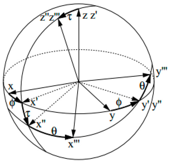
Figure 1.
Illustration of Euler angles and three axes of rotation.
The three angles are referred to as the spin angle ϕ, tilt angle τ, and rotation angle θ. For each rotation, the original axis can be represented as a new axis using a rotation matrix, and the expressions for the three rotation matrices are [50]
Based on the above equation, we can obtain the rotation matrix B, which provides the theoretical basis for the subsequent calculation of the individual particle scattering matrix.
2.2.2. Volume Scattering Model
For the modeling of scattering from forest and grass canopies, which are approximated as a cloud of randomly oriented ellipsoidal scatterers, we assume that each particle in the cloud is independent. Based on the physical model described above, we can obtain a matrix of backward scattering coefficients for the particles and their derivation equations as follows [50]:
From Equation (14),
where Bi1, Bi2, Bi3, Bk1, Bk2, and Bk3 (i,k = 1,2) are the elements in Equation (14) and ρ denotes the polarizability of the small particles. According to reciprocity, it is obtained that S12 = S21, i.e.,
By normalizing ρ and using A to denote it by taking ρ1 = 1, ρ2 = ρ3 = A, we change the particle shape by changing the value of A. For A = 1, the particle has a spherical shape or is a low-dielectric material; for A < 1, the particle has the shape of a needle; and for A > 1, the particle has the shape of a flat disk [50]. From the above calculations, we can obtain the scattering matrix S of individual particles. Then, by calculating the coherence matrix of individual particles, we can derive the volume scattering model by using the algorithm described in this paper.
From Equation (15), we can calculate the coherence matrix T of a single particle, which can be expressed as
The coherence matrix elements tij in Equation (20) are all functions of θ, ϕ, and τ, which are denoted as tij(θ, τ, ϕ). Then, the overall average coherence matrix elements ˂tij˃ of the randomly distributed ellipsoidal particles can be obtained by integrating tij (θ, τ, ϕ)sinτ over all angles as follows [50]:
According to Equations (20) and (21), we can obtain coherence matrix <T3> of the ellipsoidal particles in this algorithm as follows [50]:
Then, we derive the covariance matrix C3 in our own algorithm based on Equation (22):
Based on the aforementioned equations, we can derive the covariance matrix of the volume scattering model. In this paper, for grassland vegetation, as shown in Figure 2a, the vegetation grows uniformly, it is short and dense, and the grass leaves are slender and soft. The flat particles can be utilized to model the volume scattering components (A > 1) [51]. For forest vegetation, as shown in Figure 2b, this vegetation grows uniformly, it is tall and dense, and the needle particles can be utilized to model the volume scattering components (A < 1) [51].
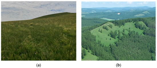
Figure 2.
Data collection on growth in areas of grassland and forest vegetation. (a) Appearance characteristics of grass; (b) Appearance characteristics of forests.
2.3. Polarimetric Target Decomposition Algorithm
SAR backscatter mainly arises from vegetation and the ground surface. In this paper, we use the above volume scattering model combined with the surface scattering component of FER2 [45] to derive the polarimetric target decomposition algorithm. We use Equation (23) to model volume scattering, and a second-order statistical covariance matrix C3V can be derived:
where the contribution of the volume scattering component is represented by ƒV. The ground scattering is modeled using FRE2 [45], and the covariance matrix C3G can be expressed as
where the contribution of the double-bounce scattering or surface scattering component is represented by ƒG and α. Then, the second-order covariance matrix C of the fully measured PolSAR data can be expressed as
According to Equation (26), we can obtain the following four equations:
By solving Equation (27), we can obtain
From Equation (32), we can calculate the magnitude of the A-value, which in turn is used to determine whether to simulate grassland or forest.
The total contribution of the various scattering mechanisms to Span is calculated as follows:
where PV denotes the volume scattering power and PG denotes the ground scattering power. When the ground scattering term is double-bounce scattering, and the parameter α satisfies |α| ≤ 1 and arg(α) = ±π, then Pd = PG; when the ground scattering term is surface scattering, and the parameter α satisfies |α| ≥ 1 and arg(α) = 2Ψ, where Ψ is the phase difference between the co-polarized HH, VV, then Ps = PG, where Pd denotes the double-bounce power and Ps denotes the surface scattering power.
2.4. Flowchart and Specific Steps of the Algorithm
The flowchart of the above adaptive polarimetric target decomposition algorithm (APD) based on A is shown in Figure 3. The specific steps are as follows:
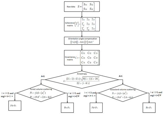
Figure 3.
The flowchart of the algorithm.
Step 1: Extract scattering matrix S from the fully measured PolSAR data using PolSARpro 6.0 software;
Step 2: Obtain coherence matrix T3 by using scattering matrix S and boxcar filtering with a 3 × 3 window for the elements of the coherence matrix to reduce speckle noise;
Step 3: Calculate θ according to Equation (7), a critical step in reducing the cross-polarization term T33, which helps to constrain the potential overestimation of volume scattering and coherence matrix T3 after orientation angle compensation is obtained from Equation (4);
Step 4: Transform coherence matrix T3 into covariance matrix C3 using Equation (8);
Step 5: Calculate A, a useful metric to determine the shape of particles and further aiding in the determination of whether volume scattering is modeled for the grass canopy or the forest canopy;
Step 6: Obtain the value of each scattering component for each pixel by calculating the target decomposition component in the polarimetric target decomposition algorithm using the value of A calculated in step 5.
3. Experimental Results and Analysis
Our intention in this study is to establish a polarimetric target decomposition algorithm that is applicable to grass volume scattering models, and we illustrate the feasibility of our proposed algorithm by comparing it with classical algorithms and some comparatively new algorithms. In order to verify the universality of APD, experiments were conducted on different bands and different types of SAR datasets: an L-band AirSAR dataset from San Francisco Bridge, a C-band AirSAR dataset from Hunshandak grassland in Inner Mongolia Autonomous Region, and an X-band COSMO-SkyMed dataset from Xiwuqi grassland in Inner Mongolia Autonomous Region.
3.1. Experiments on L-Band AirSAR Dataset
The L-band AirSAR dataset used in this paper is a four-view fully measured PolSAR dataset with a spatial resolution of 10 m and incidence angles of 5°–60° [16]. The data were downloaded from the Institute of Electronics and Telecommunications of Rennes (IETR) (URL: https://ietr-lab.univ-rennes1.fr/polsarpro-bio/san-francisco/, accessed on 2 December 2022). The original image has a size of 900 × 1024 pixels, and the Pauli RGB image is shown in Figure 4.
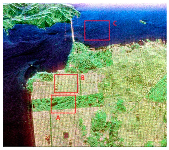
Figure 4.
Pauli RGB image from L-band San Francisco Bridge dataset. A: situated in forest; B: located in urban area; C: positioned in ocean.
We compared APD with FRE2, Y4R, MF4CF, HTCD, and GRH on the L-band AirSAR dataset to illustrate the effectiveness of the proposed algorithms. The RGB synthesis images of the above six algorithms are shown in Figure 5, with each pixel’s color represented by the double-bounce scattering power (Pd), volume scattering power (Pv), and surface scattering power (Ps). Specifically, Pd, Pv, and Ps correspond to red, green, and blue, respectively. Consequently, each pixel exhibits a color that indicates the intensity of the three scattering components. We use the color visualization in Figure 5 to compare APD with several of the algorithms described above.
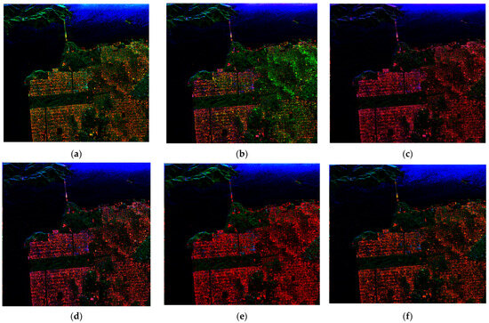
Figure 5.
RGB syntheses of polarized target decomposition algorithm. Red: double-bounce scattering (Pd); green: volume scattering (Pv); blue: surface scattering (Ps). (a) FRE2; (b) Y4R; (c) MF4CF; (d) HTCD; (e) GRH; (f) APD.
The pseudo-color map of the proposed APD is shown in Figure 5f. Based on the color visualization, it is found that the urban area’s volume scattering is overestimated, as seen in Figure 5a,b. In Figure 5c, MF4CF shows the dark color of the vegetation area, which is due to the underestimation of the volume scattering. In Figure 5d, the scattering mechanism is more reasonable compared with Figure 5c, but compared with the results of APD, the vegetation area in the middle has lower volume scattering components. In Figure 5e, GRH shows a greater red area than APD in the upper middle vegetation region and presents many double-bounce scattering components in the right vegetation triangle. Therefore, the result shown in Figure 5f is more consistent with the scattering characteristics of the region.
In order to quantitatively evaluate the scattering components, three test regions were carefully selected for use in a specific data analysis, as in Figure 4: region A, situated in the forest; region B, located in the urban area; and region C, positioned in the ocean. Each of these regions had a size of 80 × 100 pixels, and they were named region A, region B, and region C, respectively. The polarimetric target decomposition components accounted for by the various algorithms for region A, region B, and region C are given in Table 1 as percentages.

Table 1.
The percentage of each polarization component of L-band AirSAR dataset (%).
As can be observed from Table 1, in forest area A, the volume scattering power stands out as the dominant component, with the FRE2 and Y4R volume scattering percentages reaching 82.31% and 72.27%, respectively, which is due to the overestimation of volume scattering in combination with the color visualization of Figure 5. MF4CF’s volume scattering power is 55.28%, HTCD’s volume scattering power is 59.45%, GRH’s volume scattering power is 58.38%, and APD’s volume scattering power is 65.42%. APD has the highest volume scattering compared to MF4CF, HTCD, and GRH. According to the color visualization in Figure 5f, there is no overestimation of the volume scattering, which indicates that APD’s result is more consistent with the characteristics of the area.
In urban area B, double-bounce scattering is dominant and surface scattering is higher than volume scattering. For FRE2, Y4R, and GRH, the volume scattering power is higher than the surface scattering power, which is not consistent with the characteristics of the region. For MF4CF, combined with the color visualization in Figure 5c, it is found that the double-bounce scattering is overestimated. The results for HTCD and APD are more consistent with the characteristics of the region.
In marine region C, surface scattering dominates, and the percentage of surface scattering power for the six decomposition algorithms is relatively high. Among them, the proportion of double-bounce scattering power in FRE2 and GRH is not zero. From the above analysis, it can be deduced that APD is more successful in the forested area; in the urban area, the results of both HTCD and APD are consistent with the scattering characteristics of the target in the area. Moreover, in combination with the color visualization of Figure 5, it is found that the result of APD is more consistent with the scattering characteristics of every area.
For a clearer view of the results, we transformed Table 1 above into a bar chart. Figure 6 shows the bar charts for each polarization component, for all methods applied in the three regions. By combining data in Table 1 and Figure 6, we can find that APD is better than the other algorithms in terms of decomposition accuracy.
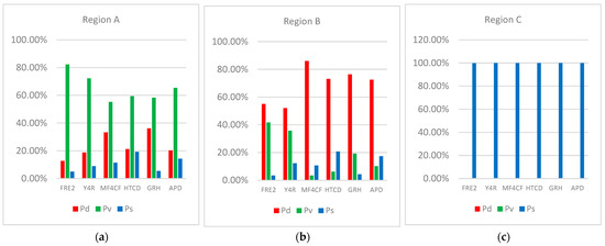
Figure 6.
Bar charts of each polarization component of L-band AirSAR dataset. (a) In forest area A; (b) In urban area B; (c) In marine region C.
3.2. Experiments on C-Band AirSAR Dataset
The C-band AirSAR dataset utilized in this section is sourced from Hunsandak grassland area, situated within Inner Mongolia Autonomous Region, with a spatial resolution of 1 m. The data were collected on 14 July 2021. The original image, which serves as the basis for our analysis, encompasses a substantial area, with dimensions of 3027 × 4096 pixels. This comprehensive image was further processed to generate a corresponding Pauli RGB map and an optical map, both of which are visually represented, in Figure 7 and Figure 8, respectively.
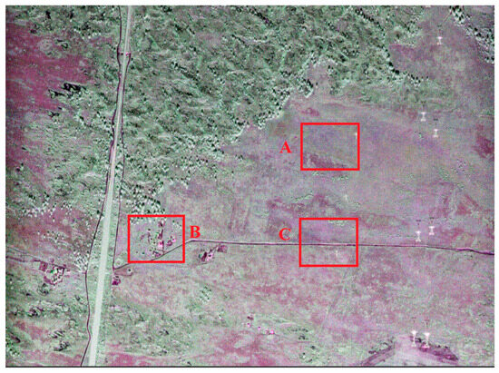
Figure 7.
Pauli RGB map of C-band Hunsandak grassland in Inner Mongolia Autonomous Region AirSAR dataset. (A): situated in vast grassland area; (B): located in urban area; (C): located on grassland road.
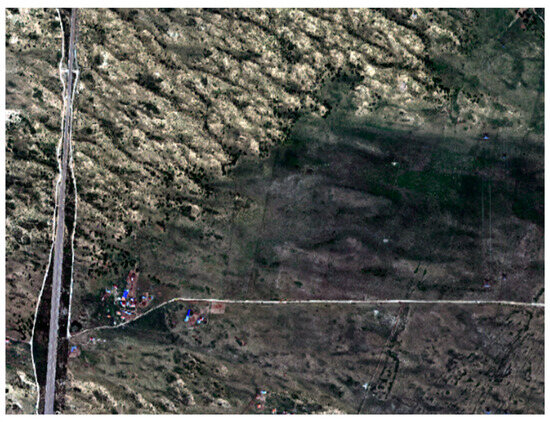
Figure 8.
Optical map of Hunsandak grassland in Inner Mongolia Autonomous Region.
The comparison methods used in the experiments described in this section are (1) FRE2, (2) Y4R, (3) MF4CF, (4) HTCD, (5) GRH, and (6) APD. The RGB syntheses of the six algorithms are shown in Figure 9. The color of each pixel is represented by the double-bounce scattering power (Pd), volume scattering power (Pv), and surface scattering power (Ps), where Pd, Pv, and Ps correspond to red, green, and blue, respectively. Thus, the color presented by each pixel indicates the intensity of the three scattering components. We also compare APD to several of the algorithms described above using the color visualization in Figure 9.
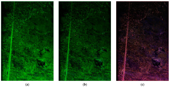
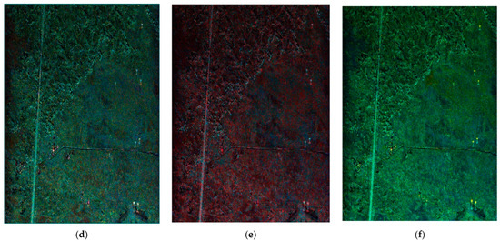
Figure 9.
RGB syntheses of polarized target decomposition algorithm. (a) FRE2; (b) Y4R; (c) MF4CF; (d) HTCD; (e) GRH; (f) APD.
The pseudo-color map of the proposed APD is shown in Figure 9f. Compared with the result of FRE2 in Figure 9a, the urban area appears redder, the road is not completely green, and there is an overestimation of the volume scattering in Figure 9a. For Y4R in Figure 9b, there is also an overestimation of the volume scattering; the red color of the RGB for MF4CF in Figure 9c and for GRH in Figure 9e is prominent, which indicates that double-bounce scattering is dominant, and it does not align with the characteristics of the grassland area. For HTCD in Figure 9d, the scattering mechanism is more reasonable; however, when comparing it with the result of APD in Figure 9f, the volume scattering of APD is better in the grassland area. Thus, Figure 9f is more reasonable, with double-bounce scattering, surface scattering in the urban area, and volume scattering and surface scattering in the grassland area.
In order to conduct a comprehensive quantitative evaluation of the scattering components, the research team strategically selected three distinct test regions for use in a specific data analysis, as depicted in Figure 7. These regions, each measuring a size of 100 × 120 pixels, are labeled as region A, region B, and region C. Region A is situated in a vast grassland area, region B is located in an urban area, and region C is located on a grassland road. Table 2 shows the percentage of each polarization component for all methods in the three regions. For a more intuitive, clearer view of the results, we transformed Table 2 above into a bar chart, shown in Figure 10. The polarimetric target decomposition components for a range of algorithms are detailed in Figure 10, indicating the percentage of components in each of the three regions.
Table 2.
The percentage of each polarization component of C-band AirSAR dataset (%).
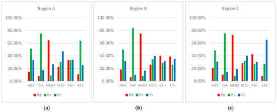
Figure 10.
Bar charts of each polarization component of C-band AirSAR dataset. (a) Situated in vast grassland area; (b) Located in urban area; (c) Located on grassland road.
For region A, the main scattering mechanisms are volume scattering and surface scattering. As can be seen in Figure 10a, FRE2, Y4R, and APD have higher volume scattering percentages relative to the other algorithms. Combined with the color visualization of Figure 7, it can be found that there is an overestimation of volume scattering in FRE2 and Y4R. MF4CF’s double-bounce scattering power percentage is much higher than that of volume scattering and surface scattering, and HTCD’s surface-scattered power percentage is greater than its volume-scattered power percentage. These two algorithms cannot match the scattering mechanism in this region. GRH is close in terms of the volume, surface, and double-bounce scattering power percentages; however, double-bounce scattering is more prominent than volume scattering, and the result does not match the target scattering characteristics of the region.
In region B, the main scattering mechanisms are double-bounce scattering and surface scattering. As can be seen in Figure 10b, for FRE2 and Y4R, the volume scattering percentages are higher, and they do not match the scattering mechanism in this region. HTCD has a higher percentage of volumetric scattering power than double-bounce scattering power, which is not consistent with the scattering characteristics of the region. Compared with the other algorithms, MF4CF has the highest percentage of double-bounce scattering. MF4CF, GRH, and APD are all dominated by surface scattering and double-bounce scattering, making their results more consistent with the scattering characteristics of the targets in the region.
In region C, the main scattering mechanisms are surface scattering and volume scattering. For FRE2 and Y4R, the volume scattering percentage is much higher than that of double-bounce scattering and surface scattering. Moreover, Figure 9 reveals that both algorithms suffer from volume scattering overestimation; thus, their results are not consistent with the scattering mechanism of this region. The MF4CF and GRH algorithms show predominantly double-bounce scattering and do not match the scattering mechanisms in the region. HTCD and APD show mainly surface scattering and volume scattering, where the surface scattering power percentage of APD is higher than the surface scattering power percentage of HTCD, so APD is more closely aligned with the scattering mechanism in this region. According to the above analysis, it is found that APD is more suitable for the grassland region.
3.3. Experiments on X-Band COSMO-SkyMed Dataset
In order to further verify the feasibility of the algorithm on high-band remote images, experiments were conducted on the X-band COSMO-SkyMed dataset from Xiwuqi in the Inner Mongolia Autonomous Region. It is pertinent to note that this region has a spatial resolution of 3 m, and the data collection date was 28 August 2023. The original image had a size of 18,663 × 7637 pixels. The corresponding Pauli RGB and optical images are shown in Figure 11.

Figure 11.
(a) Pauli RGB map of X-band Xiwuqi grassland in Inner Mongolia Autonomous RegioCOSMO-SkyMed dataset. A: located in grassland area; B: located in urban area; C: road located on grassland. (b) Optical map of part of Xiwuqi Grassland in Inner Mongolia Autonomous Region.
We compared the performance of APD with that of FRE2, Y4R, MF4CF, HTCD, and GRH on the COSMO-SkyMed dataset. The RGB syntheses of the six algorithms are shown in Figure 12. In the figure, the color of each pixel is represented by the double-bounce scattering power (Pd), volume scattering power (Pv), and surface scattering power (Pd), where Pd, Pv, and Ps correspond to red, green, and blue, respectively. Thus, the color presented by each pixel indicates the intensity of the three scattering components. We compared APD with the aforementioned algorithms based on the visual color effect shown in Figure 12.
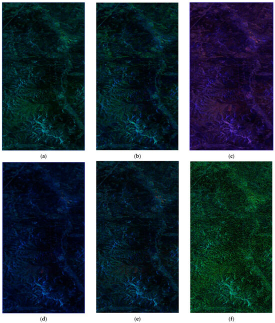
Figure 12.
RGB syntheses of polarimetric target decomposition algorithm. (a) FRE2; (b) Y4R; (c) MF4CF; (d) HTCD; (e) GRH; (f) APD.
This section proposes the use of the APD to decompose pseudo-color images, as shown in Figure 12f. Similar to FRE2 in Figure 12a and Y4R in Figure 12b, these algorithms mainly focus on volume scattering and surface scattering. Among them, FRE2 and Y4R show stronger surface scattering, while APD shows stronger volume scattering. MF4CF, as shown in Figure 12c, is mainly based on double-bounce scattering and surface scattering, and its result does not conform with the characteristics of grassland areas. Considering HTCD in Figure 12d and GRH in Figure 12e, these algorithms are mainly based on surface scattering and the results do not conform with the characteristics of grassland areas. Compared with the above results, Figure 12f shows that our algorithm is more reasonably effective and can reflect the characteristics of grassland areas.
In order to quantitatively evaluate the scattering components, three test regions were selected for use in a specific data analysis, as shown in Figure 11: region A, located in a grassland area; region B, located in an urban area; and region C, a road located on grassland. All of the test regions had a size of 100 × 200 pixels. Table 3 presents the distribution percentages of each polarization component across all methods in the three regions. To enhance data comprehension, we conducted a detailed analysis of Table 3, resulting in the compilation of a data bar chart, shown in Figure 13. The percentages of polarimetric target decomposition components of the various algorithms for region A, region B, and region C are given in Figure 13.
Table 3.
The percentages of each polarization component of X-band COSMO-SkyMed dataset (%).
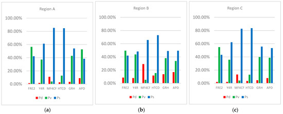
Figure 13.
Bar charts of each polarization component of X-band COSMO-SkyMed dataset. (a) Located in a grassland area; (b) Located in an urban area; (c) a road located on grassland.
For region A, the main scattering mechanisms are volume scattering and surface scattering, but volume scattering is more prominent than surface scattering. As can be seen from Figure 13a, for FRE2, Y4R, GRH, and APD, the volume scattering percentage is higher compared to other algorithms, where the surface scattering percentages of Y4R and GRH are higher than the volume scattering percentages. This does not match the scattering mechanism in this region. Similarly, MF4CF and HTCD have higher surface scattering power percentages than volume scattering power percentages and are not suitable for the target scattering characteristics in this region.
In region B, the main scattering mechanisms are double-bounce scattering and surface scattering. As shown in Figure 13b, MF4CF has the highest percentage of double-bounce scattering power compared to the other algorithms, and its surface scattering is also relatively high, which is consistent with the urban area’s scattering mechanism. Compared with the other algorithms, FRE2 and Y4R show a higher percentage of volume scattering power and lower double-bounce scattering power, which does not conform with the scattering characteristics of the target in this region. In the comparison experiments, HTCD, GRH, and APD show relatively higher percentages of surface scattering power, but APD shows higher double-bounce scattering, which is more consistent with the feature characteristics of this region.
In region C, the main scattering mechanism is surface scattering, in which there are grasses on both sides of the road, and there is volume scattering present. The percentage of volume scattering power of FRE2 is higher than that of surface scattering, which is inconsistent with the scattering mechanism in this region. The remaining algorithms Y4R, MF4CF, HTCD, GRH, and APD, are dominated by surface scattering, where the percentage of double-bounce scattering power of MF4CF is higher than its percentage of volume scattering power. Therefore, MF4CF does not match the scattering characteristics of this region. Combining the scattering target characteristics of the above three regions, it is obvious that the result of the proposed APD is more consistent with the scattering mechanism in this dataset.
We found that the scattering characteristics of different bands were different when analyzing the above AirSAR dataset in the C-band and COSMO-SkyMed dataset in the X-band, as shown in Figure 13. It was found that the three regions as a whole were dominated by surface scattering. A further analysis of the three regions in different bands of the two grassland datasets was performed. From the grassland regions shown in Figure 10a and Figure 13a, it can be seen that APD has a higher percentage of volume scattering power in the C-band data than in the X-band data, which is more consistent with the characteristics of grassland scattering. From the urban regions shown in Figure 10b and Figure 13b, it can be found that APD has a higher percentage of double-bounce scattering power than volume scattering and surface scattering for the C-band data, while the X-band data show higher volume scattering than double-bounce scattering. In Figure 10c and Figure 13c, depicting the grassland road, it is seen that the surface scattering power percentage of APD in the C-band data is much higher than that of surface scattering in the X-band data. Therefore, C-band data are more suitable for the study of scattering target characteristics in grassland.
4. Conclusions
In this paper, we present a novel adaptive polarimetric target decomposition algorithm based on the anisotropy degree to simulate the scattering mechanisms of grasslands and forests. Compared with FER2, Y4R, MF4CF, HTCD, and GRH, the volume scattering model of APD is more consistent with the characteristics of various terrain features, effectively improving the volume scattering model. By applying the model to an L-band AirSAR dataset from San Francisco Bridge, it is found that the forest’s volume scattering can be successfully simulated by changing the value of A so that the particle shape is a needle. On a C-band AirSAR dataset from Hunshandak grassland in Inner Mongolia Autonomous Region, it is found that when the particle shape is changed to a disk, the scattering mechanism of the grassland area can be better simulated. In order to further verify the reliability of this algorithm, an X-band COSMO-SkyMed dataset from Xiwuqi, Inner Mongolia Autonomous Region was used for verification, and it is found that APD better reflects the grassland region compared to the other algorithms applied in the experiments. The results show that C-band data are more suitable for the study of scattering target characteristics in grasslands.
With the deepening research on polarimetric target decomposition algorithms, various methods have emerged. Although these algorithms have achieved significant results, the complexity of polarimetric SAR data leads to shortcomings. The environment is complex, and the distinction between the scattering mechanisms is not clear, especially in grassland areas. In future research, the combination of polarimetric decomposition with deep learning could improve the classification accuracy.
Author Contributions
Conceptualization, P.H. and B.L.; methodology, P.H. and B.L.; software, P.H. and B.L.; investigation, X.L. and W.T.; visualization, P.H. and X.L.; writing—original draft preparation, P.H. and W.X.; writing—review and editing, X.L., W.T. and Y.C.; project administration, P.H. and X.L. All authors have read and agreed to the published version of the manuscript.
Funding
This work was supported in part by the Joint Funds of the National Natural Science Foundation of China (Nos. U22A2010); in part by the Center for Applied Mathematics of Inner Mongolia (Nos. ZZYJZD2022001); and in part by the National Natural Science Foundation of China (Nos. 62071258, 52064039 and 52304173).
Data Availability Statement
The data presented in this study are available on request from the corresponding author. The data are not publicly available due to privacy.
Conflicts of Interest
The authors declare no conflicts of interest.
References
- Ali, I.; Cawkwell, F.; Dwyer, E.; Barrett, B.; Green, S. Satellite remote sensing of grasslands: From observation to management. J. Plant Ecol. 2016, 9, 649–671. [Google Scholar] [CrossRef]
- Hajnsek, I.; Jagdhuber, T.; Schon, H.; Papathanassiou, K.P. Potential of Estimating Soil Moisture Under Vegetation Cover by Means of PolSAR. IEEE Trans. Geosci. Remote Sens. 2009, 47, 442–454. [Google Scholar] [CrossRef]
- Sun, Y.; Montazeri, S.; Wang, Y.; Zhu, X.X. Automatic registration of a single SAR image and GIS building footprints in a large-scale urban area. ISPRS J. Photogramm. Remote Sens. 2020, 170, 1–14. [Google Scholar] [CrossRef]
- Chen, G.; Wang, L.; Kamruzzaman, M.M. Spectral Classification of Ecological Spatial Polarization SAR Image Based on Target Decomposition Algorithm and Machine Learning. Neural. Comput. Appl. 2020, 32, 5449–5460. [Google Scholar] [CrossRef]
- Alvarez-Perez, J.L. Coherence, Polarization, and Statistical Independence in Cloude–Pottier’s Radar Polarimetry. IEEE Trans. Geosci. Remote Sens. 2011, 49, 426–441. [Google Scholar] [CrossRef]
- Song, Q.; Xu, F. Polarimetric SAR Target Decomposition based on sparse NMF. In Proceedings of the 2016 Progress in Electromagnetic Research Symposium (PIERS), Shanghai, China, 8–11 August 2016. [Google Scholar] [CrossRef]
- Chen, S.; Wang, X.; Xiao, S. Urban Damage Level Mapping Based on Co-Polarization Coherence Pattern Using Multitemporal Polarimetric SAR Data. IEEE J. Sel. Top. Appl. Earth Obs. Remote Sens. 2018, 11, 2657–2667. [Google Scholar] [CrossRef]
- Chen, S.; Wang, X.; Sato, M. Urban Damage Level Mapping Based on Scattering Mechanism Investigation Using Fully Polarimetric SAR Data for the 3.11 East Japan Earthquake. IEEE Trans. Geosci. Remote Sens. 2016, 54, 6919–6929. [Google Scholar] [CrossRef]
- Musthafa, M.; Khati, U.; Singh, G. Sensitivity of PolSAR decomposition to forest disturbance and regrowth dynamics in a managed forest. Adv. Space Res. 2020, 66, 1863–1875. [Google Scholar] [CrossRef]
- Varghese, A.O.; Suryavanshi, A.; Joshi, A.K. Analysis of different polarimetric target decomposition methods in forest density classification using C band SAR data. Int. J. Remote Sens. 2016, 37, 694–709. [Google Scholar] [CrossRef]
- Acar, H.; Ozerdem, M.S.; Acar, E. Soil Moisture Inversion Via Semiempirical and Machine Learning Methods with Full-Polarization Radarsat-2 and Polarimetric Target Decomposition Data: A Comparative Study. IEEE Access 2020, 8, 197896–197907. [Google Scholar] [CrossRef]
- Zhang, L.; Meng, Q.; Zeng, J.; Wei, X.; Shi, H. Evaluation of Gaofen-3 C-Band SAR for Soil Moisture Retrieval Using Different Polarimetric Decomposition Models. IEEE J. Sel. Top. Appl. Earth Obs. Remote Sens. 2021, 14, 5707–5719. [Google Scholar] [CrossRef]
- Zhang, X.; Xu, J.; Chen, Y.; Xu, K.; Wang, D. Coastal Wetland Classification with GF-3 Polarimetric SAR Imagery by Using Object-Oriented Random Forest Algorithm. Sensors 2021, 21, 3395. [Google Scholar] [CrossRef] [PubMed]
- Cloude, S.R.; Pottier, E. A Review of Target Decomposition Theorems in Radar Polarimetry. IEEE Trans. Geosci. Remote Sens. 1996, 34, 498–518. [Google Scholar] [CrossRef]
- Wang, Y.; Yu, W.; Wang, C.; Liu, X. A Modified Four-Component Decomposition Method With Refined Volume Scattering Models. IEEE J. Sel. Top. Appl. Earth Obs. Remote Sens. 2020, 13, 1946–1958. [Google Scholar] [CrossRef]
- Yamaguchi, Y.; Yajima, Y.; Yamada, H. A Four-Component Decomposition of POLSAR Images Based on the Coherency Matrix. IEEE Geosci. Remote Sens. Lett. 2006, 3, 292–296. [Google Scholar] [CrossRef]
- Sato, A.; Yamaguchi, Y.; Singh, G.; Park, S.-E. Four-Component Scattering Power Decomposition with Extended Volume Scattering Model. IEEE Geosci. Remote Sens. Lett. 2012, 9, 166–170. [Google Scholar] [CrossRef]
- Kumar, A.; Maurya, H.; Misra, A.R.; Panigrahi, R.K. An Improved Decomposition as a Trade-Off Between Utilizing Unitary Matrix Rotations and New Scattering Models. IEEE Access 2021, 9, 77482–77492. [Google Scholar] [CrossRef]
- Freeman, A.; Durden, S.L. Three-component scattering model to describe polarimetric SAR data. In Proceedings of the International Society for Optics and Photonics, San Diego, CA, USA, 12 February 1993. [Google Scholar] [CrossRef]
- Jagdhuber, T.; Hajnsek, I.; Papathanassiou, K.P. An Iterative Generalized Hybrid Decomposition for Soil Moisture Retrieval Under Vegetation Cover Using Fully Polarimetric SAR. IEEE J. Sel. Top. Appl. Earth Obs. Remote Sens. 2015, 8, 3911–3922. [Google Scholar] [CrossRef]
- Van Zyl, J.J.; Arii, M.; Kim, Y. Requirements for Model-Based Polarimetric Decompositions. In Proceedings of the International Geoscience and Remote Sensing Symposium (IGARSS), Boston, MA, USA, 8–11 July 2008; IEEE: New York, NY, USA, 2008; Volume 5, pp. 417–420. [Google Scholar]
- Van Zyl, J.J.; Arii, M.; Kim, Y. Model-based Decomposition of Polarimetric SAR Covariance Matrices Constrained for Nonnegative Eigenvalues. IEEE Trans. Geosci. Remote Sens. 2011, 49, 3452–3459. [Google Scholar] [CrossRef]
- Lee, J.S.; Ainsworth, T.L. The Effect of Orientation Angle Compensation on Coherency Matrix and Polarimetric Target Decompositions. IEEE Trans. Geosci. Remote Sens. 2011, 49, 53–64. [Google Scholar] [CrossRef]
- Yin, J.; Yang, J. Target Decomposition Based on Symmetric Scattering Model for Hybrid Polarization SAR Imagery. IEEE Geosci. Remote Sens. Lett. 2021, 18, 494–498. [Google Scholar] [CrossRef]
- Chen, S.-W.; Li, Y.-Z.; Wang, X.-S.; Xiao, S.-P.; Sato, M. Modeling and Interpretation of Scattering Mechanisms in Polarimetric Synthetic Aperture Radar: Advances and perspectives. IEEE Signal Process. Mag. 2014, 31, 79–89. [Google Scholar] [CrossRef]
- Cloude, S.R. Polarisation: Applications in Remote Sensing; Oxford University Press: New York, NY, USA, 2010. [Google Scholar]
- Singh, G.; Yamaguchi, Y.; Park, S.; Cui, Y.; Kobayashi, H. Hybrid Freeman/Eigenvalue Decomposition Method with Extended Volume Scattering Model. IEEE Geosci. Remote Sens. Lett. 2013, 10, 81–85. [Google Scholar] [CrossRef]
- Maurya, H.; Bhattacharya, A.; Mishra, A.K.; Panigrahi, R.K. Hybrid Three-Component Scattering Power Characterization From Polarimetric SAR Data Isolating Dominant Scattering Mechanisms. IEEE Trans. Geosci. Remote Sens. 2022, 60, 1–15. [Google Scholar] [CrossRef]
- Chen, S.-W.; Sato, M. Tsunami Damage Investigation of Built-Up Areas Using Multitemporal Spaceborne Full Polarimetric SAR Images. IEEE Trans. Geosci. Remote Sens. 2013, 51, 1985–1997. [Google Scholar] [CrossRef]
- Yamaguchi, Y.; Sato, A.; Boerner, W.; Sato, R.; Yamada, H. Four-component scattering power decomposition with rotation of coherency matrix. IEEE Trans. Geosci. Remote Sens. 2011, 49, 2251–2258. [Google Scholar] [CrossRef]
- Xiang, D.; Ban, Y.; Su, Y. Model-Based Decomposition with Cross Scattering for Polarimetric SAR Urban Areas. IEEE Geosci. Remote Sens. Lett. 2015, 12, 2496–2500. [Google Scholar] [CrossRef]
- Hu, C.; Wang, Y.; Sun, X.; Quan, S.; Xiang, D. Model-Based Polarimetric Target Decomposition with Power Redistribution for Urban Areas. IEEE J. Sel. Top. Appl. Earth Obs. Remote Sens. 2023, 16, 8795–8808. [Google Scholar] [CrossRef]
- Wang, Y.; Yu, W.; Liu, X.; Wang, C. Seven-Component Decomposition Using Refined Volume Scattering Models and New Configurations of Mixed Dipoles. IEEE J. Sel. Top. Appl. Earth Obs. Remote Sens. 2020, 13, 4339–4351. [Google Scholar] [CrossRef]
- Zhang, S.; Yu, X.; Wang, L. Modified version of three-component model-based decomposition for polarimetric SAR data. J. Syst. Eng. Electron. 2019, 30, 270–277. [Google Scholar] [CrossRef]
- Han, W.; Fu, H.; Zhu, J.; Wang, C.; Xie, Q. Polarimetric SAR Decomposition by Incorporating a Rotated Dihedral Scattering Model. IEEE Geosci. Remote Sens. Lett. 2022, 19, 1–5. [Google Scholar] [CrossRef]
- Yue, X.; Teng, F.; Lin, Y.; Hong, W. Target Scattering Feature Extraction Based on Parametric Model Using Multi-Aspect SAR Data. Remote Sens. 2023, 15, 1883. [Google Scholar] [CrossRef]
- Arii, M.; van Zyl, J.J.; Kim, Y. Adaptive Model-Based Decomposition of Polarimetric SAR Covariance Matrices. IEEE Trans. Geosci. Remote Sens. 2010, 49, 1104–1113. [Google Scholar] [CrossRef]
- Chen, S.-W.; Wang, X.-S.; Xiao, S.-P.; Sato, M. General Polarimetric Model-Based Decomposition for Coherency Matrix. IEEE Trans. Geosci. Remote Sens. 2013, 52, 1843–1855. [Google Scholar] [CrossRef]
- Bhattacharya, A.; Singh, G.; Manickam, S.; Yamaguchi, Y. An adaptive general four-component scattering power decomposition with unitary transformation of coherency matrix (AG4U). IEEE Geosci. Remote Sens. Lett. 2015, 12, 2110–2114. [Google Scholar] [CrossRef]
- Cui, Y.; Yamaguchi, Y.; Yang, J.; Park, S.-E.; Kobayashi, H.; Singh, G. Three-Component Power Decomposition for Polarimetric SAR Data Based on Adaptive Volume Scatter Modeling. Remote Sens. 2012, 4, 1559–1572. [Google Scholar] [CrossRef]
- Chen, S.-W.; Wang, X.-S.; Li, Y.-Z.; Sato, M. Adaptive Model-Based Polarimetric Decomposition Using PolInSAR Coherence. IEEE Trans. Geosci. Remote Sens. 2013, 52, 1705–1718. [Google Scholar] [CrossRef]
- Wang, Y.; Yu, W.; Liu, X.; Wang, C.; Kuijper, A.; Guthe, S. Demonstration and Analysis of an Extended Adaptive General Four-Component Decomposition. IEEE J. Sel. Top. Appl. Earth Obs. Remote Sens. 2020, 13, 2573–2586. [Google Scholar] [CrossRef]
- Wang, T.; Suo, Z.; Jiang, P.; Ti, J.; Ding, Z.; Qin, T. An Optimal Polarization SAR Three-Component Target Decomposition Based on Semi-Definite Programming. Remote Sens. 2023, 15, 5292. [Google Scholar] [CrossRef]
- Wang, Z.; Zeng, Q.; Jiao, J. An Adaptive Decomposition Approach with Dipole Aggregation Model for Polarimetric SAR Data. Remote Sens. 2021, 13, 2583. [Google Scholar] [CrossRef]
- Freeman, A. Fitting a Two-Component Scattering Model to Polarimetric SAR Data from Forests. IEEE Trans. Geosci. Remote Sens. 2007, 45, 2583–2592. [Google Scholar] [CrossRef]
- Dey, S.; Bhattacharya, A.; Frery, A.C.; Lopez-Martinez, C.; Rao, Y.S. A Model-Free Four Component Scattering Power Decomposition for Polarimetric SAR Data. IEEE J. Sel. Top. Appl. Earth Obs. Remote Sens. 2021, 14, 3887–3902. [Google Scholar] [CrossRef]
- Maurya, H.; Panigrahi, R.K. Non-negative scattering power decomposition for PolSAR data interpretation. IET Radar Sonar Navig. 2018, 12, 593–602. [Google Scholar] [CrossRef]
- Li, X.; Liu, Y.; Huang, P.; Liu, X.; Tan, W.; Fu, W.; Li, C. A Hybrid Polarimetric Target Decomposition Algorithm with Adaptive Volume Scattering Model. Remote Sens. 2022, 14, 2441. [Google Scholar] [CrossRef]
- Maurya, H.; Panigrahi, R.K. PolSAR Coherency Matrix Optimization Through Selective Unitary Rotations for Model-Based Decomposition Scheme. IEEE Geosci. Remote Sens. Lett. 2018, 16, 658–662. [Google Scholar] [CrossRef]
- Manuel, L. Analysis and Estimation of Biophysical Parameters of Vegetation by Radar Polarimetry. Ph.D. Thesis, Universidad Politecnica de Valencia, Valencia, Spain, 2000. [Google Scholar]
- Liu, L. Research on Composite Electromagnetic Scattering from Grass-Containing Rough Surfaces and Targets; Xidian University: Xi’an, China, 2020. [Google Scholar] [CrossRef]
Disclaimer/Publisher’s Note: The statements, opinions and data contained in all publications are solely those of the individual author(s) and contributor(s) and not of MDPI and/or the editor(s). MDPI and/or the editor(s) disclaim responsibility for any injury to people or property resulting from any ideas, methods, instructions or products referred to in the content. |
© 2024 by the authors. Licensee MDPI, Basel, Switzerland. This article is an open access article distributed under the terms and conditions of the Creative Commons Attribution (CC BY) license (https://creativecommons.org/licenses/by/4.0/).