Synthetic Aperture Radar Radio Frequency Interference Suppression Method Based on Fusing Segmentation and Inpainting Networks

Abstract

Synthetic Aperture Radar (SAR) is a high-resolution imaging sensor commonly mounted on platforms such as airplanes and satellites for widespread use. In complex electromagnetic environments, radio frequency interference (RFI) severely degrades the quality of SAR images due to its widely varying bandwidth and numerous unknown emission sources. Although traditional deep learning-based methods have achieved remarkable results by directly processing SAR images as visual ones, there is still considerable room for improvement in their performance due to the wide coverage and high intensity of RFI. To address these issues, this paper proposes the fusion of segmentation and inpainting networks (FuSINet) to suppress SAR RFI in the time-frequency domain. Firstly, to weaken the dominance of RFI in SAR images caused by high-intensity interference, a simple CCN-based network is employed to learn and segment the RFI. This results in the removal of most of the original interference, leaving blanks that allow the targets to regain dominance in the overall image. Secondly, considering the wide coverage characteristic of RFI, a U-former network with global information capture capabilities is utilized to learn the content covered by the interference and fill in the blanks created by the segmentation network. Compared to the traditional Transformer, this paper enhances its global information capture capabilities through shift-windows and down-sampling layers. Finally, the segmentation and inpainting networks are fused together through a weighted parameter for joint training. This not only accelerates the learning speed but also enables better coordination between the two networks, leading to improved RFI suppression performance. Extensive experimental results demonstrate the substantial performance enhancement of the proposed FuSINet. Compared to the PISNet+, the proposed attention mechanism achieves a 2.49 dB improvement in peak signal-to-noise ratio (PSNR). Furthermore, compared to Uformer, the FuSINet achieves an additional 4.16 dB improvement in PSNR.

1. Introduction

Synthetic aperture radar (SAR) is a high-resolution imaging radar, whose resolution can surpass the diffraction limit of the aperture, and even reach the centimeter level [1,2]. SAR satellites with various frequency bands have been widely deployed, including the European Sentinel satellites, Chinese Haisi satellites, and the Canadian Radarsat satellites [3]. While SAR satellites hold significant economic value in ocean monitoring, geospatial mapping, and target recognition [4,5,6], they also face complex electromagnetic interference. Common interference sources include co-frequency radars, satellite communication systems, and radar jammers [7,8]. Radio frequency interference (RFI) is a prevalent pattern, and because of its high intensity and wide coverage, it severely degrades the quality of SAR images [9]. Figure 1 shows a common RFI in Sentinel-1 satellites, with interference region typically exceeding 0.5 million pixels, corresponding to areas larger than 30 square kilometers.

Satellite cross-interference and military conflicts can lead to SAR satellite blindness. To solve the above problems, numerous methods have been proposed. According to the different stages of anti-interference, radar anti-interference can be divided into system-level anti-interference and signal-level anti-interference. System-level anti-interference technology mainly uses array antennas to cancel interference, and this technology has achieved long-term development. However, SAR is a single-antenna radar imaging system, and currently deployed SAR satellites generally lack system-level anti-interference capability. In addition, the overlap between interference signals and radar signals in time and frequency is high, and simple filtering algorithms are difficult to be effective. Therefore, signal-level anti-interference technology has important research value.

Traditional interference suppression methods can be broadly classified into three categories: non-parametric methods, parametric methods, and semi-parametric methods [10]. Non-parametric methods mainly include subspace projection [11,12,13] and notch filtering [14,15,16,17,18]. Although non-parametric methods are simple to implement, they lack protection for targets. Parametric methods are required to model RFI signals, and in complex imaging scenarios, the performance is constrained by the models [19]. Instead of directly modeling the RFI, semi-parametric interference suppression algorithms establish an optimization model to perform matrix decomposition. Semi-parametric methods can effectively eliminate interference while maximizing target preservation, thus receiving widespread attention. With the rise of compressive sensing, sparse reconstruction algorithms have gradually become a commonly used semi-parametric method [20]. The earliest proposals for mitigating RFI using iterative models were made by Nguyen [21] and Nguyen and Tran [22], who explored the sparsity of scenes and the correlation between transmitted and received signals in the time domain, and proposed a sparse recovery theory applicable to SAR images. By utilizing different characteristics in various domains (image domain, time domain, Doppler domain, wavelet domain, etc.), various iterative relations and models have been explored, including sparse models [23,24], low-rank models [25,26], joint sparse low-rank models [27,28,29,30,31], and variations in robust PCA [32,33]. Although the aforementioned semi-parametric algorithms have achieved excellent performance, they require iterations for each individual data with the selection of specific hyperparameters, resulting in high computational complexity and poor generalization ability.

Based on deep learning, interference suppression methods have also gained widespread attention, but they still face two major challenges. First, RFI holds a wide coverage and high interference intensity, making it difficult to be removed in the image domain. However, in the signal domain, the overlap between the targets and interference may not be very high. Therefore, one challenge is how to find a transformation domain with higher discrimination between the targets and interference. Second, although the performance of deep learning has surpassed traditional methods such as robust PCA, the published networks have limited capability in extracting prior information. Therefore, there is still significant room for improvement. To address these issues, this paper proposes a robust RFI network (FuSINet), the performance of which is shown in Figure 2, and the innovations are as follows:

1. It is challenging to eliminate RFI in the image domain due to its high interference intensity and wide coverage. Based on the analysis of radar signals, it is found that the overlap between targets and interference is relatively low in the time-frequency domain. Therefore, a time-frequency domain interference suppression method is proposed in this paper, and RFI suppression is integrated into the SAR imaging process.

2. Based on the time-frequency analysis of radar signals and interference signals, it is found that the signals hold global characteristics on the time-frequency graph. Therefore, a Transformer-based network can better capture global information. And the computational cost is reduced by adopting a non-overlapping window attention mechanism. Additionally, by analyzing the distribution characteristics of RFI, we found that variable interference components have a negative contribution to image restoration. Therefore, it inspires us to remove the interference before restoration by modifying the network structure and reconstructing the loss function.

3. The experimental results demonstrate a significant performance improvement. Compared to the PISNet+, the global attention mechanism achieves a 2.49 dB improvement in PSNR. Furthermore, compared to the global attention network, the proposed FuSINet achieves an additional 4.16 dB improvement in PSNR.

The organization of this paper is as follows: Section 2 introduces the related work. Section 3 presents the method. Section 4 presents the experimental results. Section 5 provides a summary of the entire paper.

2. Related Works

2.1. Interference Suppression Networks

SAR is a type of microwave imaging radar, and RFI produces similar noise effects in images, so deep learning has been naturally introduced into SAR interference suppression. In terms of the image domain, refs. [34,35] introduce residual networks and attention mechanisms into the networks. However, these algorithms lack an understanding of SAR principles and only treat interference as noise. When interference intensity is high, the performance is poor. In the time-frequency domain, ref. [36] introduces neural networks for the first time in interference suppression. The authors of [37] propose to adopt properties of RFI and SAR data as prior knowledge to inject into the network; this algorithm achieves better performance than traditional non-deep learning methods (including semi-parametric methods) and it serves as one of the main comparative methods in this paper.

2.2. Transformer

Transformer has achieved great success in natural language processing (NLP), especially in GPTs [38,39,40] and ChatGPT [41]. Unlike CNN architecture, Transformer-based networks hold global attention mechanisms, making it easier to capture global information. Pretrained models based on BERT [42,43] have demonstrated state-of-the-art performance in various downstream NLP tasks. These results indicate that the Transformer holds excellent feature extraction capabilities, which naturally inspires other tasks such as computer vision. In visual tasks, the pioneering work of VIT [44,45] achieves state-of-the-art results in the image classification task.

Although Transformer has shown great success in many tasks, it also presents two limitations in visual tasks. First, visual tasks often involve high redundancy and large amounts of data, resulting in significant computational costs. Second, local information is often important, but Transformer lacks the ability to capture local information. To address the first limitation, some works [46,47,48] explore local attention windows to reduce computational costs. Other works employ mask mechanisms and discard most mask pixels to reduce computational costs [49]. To address the second limitation, some works propose a pyramid Transformer [50,51] to enable multi-dimensional information interaction. Also, some works combine Transformer with CNN in network architectures to capture both local and global information. Due to the excellent feature extraction capabilities, a series of Transformer-based models have been proposed in high-dimensional visual tasks [52,53] and low-dimensional generative tasks [48,54].

3. Approach

The main body of the proposed SAR RFI suppression approach based on fusing seg-mentation and inpainting networks is presented in this section. Section 3.1 discusses the mathematical principles of radio frequency interference. Section 3.2 describes the pipeline of RFI suppression, where the diagram of the whole of the proposed method is present. The detail of the fusion of segmentation and inpainting network is given in Section 3.3.

3.1. Mathematical Principles of RFI

Common RFI can be divided into narrowband interference and wideband interference, with the latter further categorized into chirp-modulated wideband interference and sinusoidal-modulated wideband interference. Narrowband interference can be represented as follows:

$$s_{\mathrm{nbi}}\left(t\right)={\displaystyle {\sum }_{n=1}^N{A}_n\exp \left(j2\pi f_{c}t+j2\pi f_{n}t\right)},$$

(1)

where $f_c$, $A_n$, and $f_n$ are sequentially represented as carrier frequency, the amplitude of the n-th interference signal, and the frequency offset of the n-th interference signal, which is the number of interference signals. The chirp modulation interference can be represented as follows:

$$s_{{\mathrm{wbi}}_{\mathrm{cm}}}\left(t\right)={\displaystyle {\sum }_{n=1}^N{B}_n\exp \left(j2\pi f_{c}t+j\pi k_n{t}^2\right)},$$

(2)

where $B_n$ and $k_n$ are sequentially represented as the amplitude of the n-th interference signal, and the chirp rate of the n-th interference signal. The sinusoidal modulation interference can be represented as follows:

$$s_{{\mathrm{wbi}}_{\mathrm{sm}}}\left(t\right)={\displaystyle {\sum }_{n=1}^N{C}_n\exp \left(j2\pi f_{c}t+{\beta }_n\sin \left(2\pi f_{n}t\right)\right)},$$

(3)

where $C_n$, ${\beta }_n$, and $f_n$ are sequentially represented as the amplitude of the n-th interference signal, carrier frequency, modulation coefficient of the n-th interference signal, and modulation frequency of the n-th interference signal.

According to the Bessel formula, sinusoidal modulated broadband interference can be expressed as follows:

$$\begin{array}{l}{s}_{{\mathrm{wbi}}_{\mathrm{sm}}}\left(t\right)={\displaystyle {\sum }_{n=1}^N\left(C_n\exp \left(j2\pi f_{c}t+{\beta }_n\sin \left(2\pi f_{n}t\right)\right)\right)}\\ ={\displaystyle {\sum }_{n=1}^N\left(C_n{\displaystyle {\sum }_{m=-\infty }^{m=\infty }\left({\beta }_n\sin \left(2\pi f_{c}t+2\pi m{f}_{n}t\right)+{\beta }_n\cos \left(2\pi f_{c}t+2\pi m{f}_{n}t\right)\right)}\right)}\end{array},$$

(4)

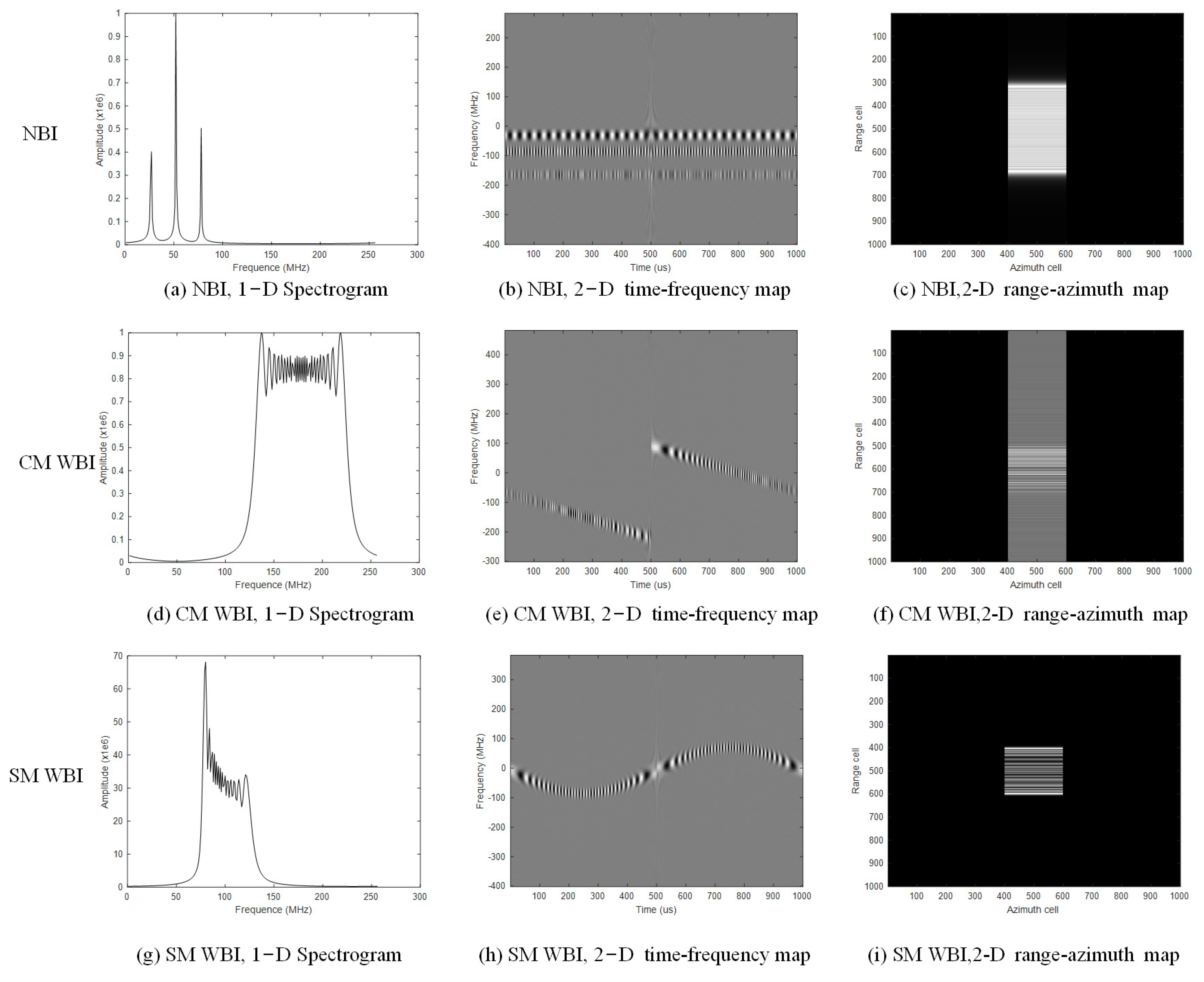
According to Equation (4), sinusoidal modulated broadband interference is composed of a series of narrowband interferences, approximating a specific form of chirp modulated broadband interference. The spectrum and time-frequency graphs of the interference signals are illustrated in Figure 3. Each row represents a type of interference paradigm, where the first row represents narrowband interference, the second row represents chirp modulation interference, and the third row represents sinusoidal modulation interference. Each column represents a representation dimension of the interference signal, with the first column depicting the interference spectrum, the second column displaying the time-frequency map of the interference, and the third column displaying the interfered SAR images.

To simplify the analysis, the radio frequency interference signal can be unified and represented as follows:

$$s_{rfi}\left(t\right)=\exp \left(j2\pi f_{c}t+j\pi k_{rfi}{t}^2\right),$$

(5)

where $k_{rfi}$ is tuning rate, $k_{rfi}\cdot t_r$ is the bandwidth of interference; when $k_{rfi}$ is large, the interference signal is a broadband signal, and when $k_{rfi}$ is small, the interference signal is a narrowband signal.

The range matched filter is given by the following:

$$h_{mf}\left(t\right)=\exp \left(j2\pi f_{c}t+j\pi k_r{t}^2\right),$$

(6)

After performing range-matched filtering, RFI can be expressed as follows:

$$s_{rfi\_mf}\left(t\right)={\displaystyle {\int }_{-\infty }^{\infty }{s}_{rfi}\left(\tau \right)}{h}_{mf}\left(t-\tau \right)d\tau =rect\left(\frac{t}{t_r}\right)\exp \left(j\pi \left(k_{rfi}-k_r\right)t^2\right),$$

(7)

According to Equation (7), after matched filtering, the interference signal is also a wideband signal, which appears as a block-like coverage.

3.2. RFI Suppression Pipeline

The RFI suppression pipeline is schematically represented in Figure 4, where the interference image undergoes Fourier transformation and is subsequently divided into two paths. One path involves the amplitude spectrum, which passes through two cascaded networks to suppress interference, while the other path concerns the phase spectrum, which remains unchanged or has slight adjustments. Following the processing of both paths, the results are recombined and undergo inverse Fourier transformation to reconstruct the azimuth-range image. The specific details are as follows.

As SAR images are like visual data, visual image inpainting methods based on neural networks are becoming more and more popular for suppressing SAR RFI. In this framework, the image inpainting model based on maximum posterior probability can be formulated as follows:

$$\underset{Y}{\max }\log \left(P\left(Y/X\right)\right)\propto \log \left(P\left(X/Y\right)\right)+\log \left(P\left(Y\right)\right),$$

(8)

where X and Y represent the disturbed image and inpainting image, respectively; log(P(X/Y)) denotes the loss function and $\log \left(P\left(Y\right)\right)$ is the prior information of X. Equation (8) can be compactly expressed as follows:

$$\underset{X}{\min }l\left(X,Y\right)+\lambda R\left(Y\right).$$

(9)

From Equation (9), one can see that with more prior information, higher performance can be achieved while using the same model. In fact, the motivation of most famous deep neural networks is to mine the prior information of the data to be dealt with.

Using Equations (6) and (7) from Section 3.1, the relationship between frequency and time is as follows:

$$f_{rfi}=k_{rfi}\cdot t,$$

(10)

$$f_{radar}=k_r\cdot t.$$

(11)

According to Equations (10) and (11), both the target signal and RFI signal appear as linear functions over time, leading to global characteristics in the time-frequency domain. We state that this is an obvious prior information that can help us achieve better performance of RFI suppression.

Prior1. Both the interference signal and the target signal hold global features.

Prior1 guides us to seek a network that can capture global feature information to achieve interference suppression. In the prosperous field of deep learning with various network models, adjusting existing models is a better choice compared to designing a delicate neural network from scratch since it can also achieve very good results in most cases. Based on this, we choose U-Transformer (Uformer) with an attention mechanism and the ability to capture fine texture information as the backbone network.

The cornerstone of transformer-based methods is the attention mechanism which allows for parallel computation of the similarity between every interested token or query token and other tokens without limitations on distance. Here, a token usually refers to the linear mapping (embedding by matrix) of image patches in the time-frequency diagram. By visualizing and analyzing the output content of various layers of deep neural networks, there is increasing evidence that transformer-based image inpainting can generate content for the damaged areas that do not have semantic conflicts with the entire image. The crucial semantics mainly refer to edge contours or geometric structures within the damaged areas, which are often referred to as latent patterns in high-level image processing tasks such as classification, recognition, segmentation, and more. Therefore, to generate desirable undistorted content for the interfered area, we need to extract patterns of the original image content from undisturbed areas that are below the interfered areas.

It is assumed that $\{{\pi }_1,\cdots ,{\pi }_{Z_1}\}$ and $\{{\phi }_1,\cdots ,{\phi }_{Z_2}\}$ are sets of Z₁ + Z₂ distinct patterns embranced in the training data set, where ${\pi }_i,i\in \left[Z_1\right]$ and ${\phi }_j,j\in \left[Z_2\right]$ come from clean and RFI regions of disturbed SAR images, respectively. Since $\{{\pi }_1,\cdots ,{\pi }_{Z_1}\}$ is beneficial to reconstructing the damaged SAR image, we call ${\pi }_i,i\in \left[Z_1\right]$ train-related pattern. Accordingly, ${\phi }_j,j\in \left[Z_2\right]$ is a train-unrelated pattern due to he negative effect on reconstruction. A token used to train a Transformer can be represented as

$$x_k^{(n)}={\alpha }_k^{(n)}{\pi }_i+{\beta }_k^{(n)}{\phi }_j+n_k^{(n)},$$

(12)

where superscript $n\in [N]$ and subscript $k\in [K]$ indicate that the kth token is extracted from nth training sample; $n_i^{(n)}$ is gaussian noise $\mathcal{N}(0,{\sigma }^2)$ iid for different i and n; ${\alpha }^{*}=\underset{k,n}{\min }({\alpha }_k^{(n)})$ and $\overline{\alpha }={\displaystyle {\sum }_n{\displaystyle {\sum }_k{\alpha }_k^{(n)}}}$ denote the minimum and mean fraction of train-related patterns, respectively. Ref. [55] states the following theorem.

Theorem 1.

For a self-attention-based transformer whose attention block is followed by a feed-forward network, as long as the number of neurons m is large enough that $m\ge {(c_1{Z}_1)}^2\log N$ for constant $c_1\ge 2$, the mini-batch size $B>\Omega (Z_1\log Z_1)$. Then, after

$$T=\Theta \left(\frac{1}{{\alpha }^{*}\overline{\alpha }{c}_2}\sqrt{\frac{Z_1+Z_2}{1-c_1^{-1}-\sigma Z_1}}\right),$$

(13)

the number of iterations, the trained model achieves zero generalization error with a sufficiently large probability. c₁ and c₂ are some constants related to the characteristics of the dataset. $u(\cdot )=\Omega \left(v(\cdot )\right)$ and $u(\cdot )=\Theta \left(v(\cdot )\right)$ indicate that $u(\cdot )$ increases at least or in the order of $v(\cdot )$, respectively.

From Theorem 1, the sample complex N = TB can be a reduced scale with $1/{\alpha }^{*}$ or $1/\overline{\alpha }$. On the other hand, while N = TB remains unchanged, lower $1/{\alpha }^{*}$ or $1/\overline{\alpha }$ means higher generalization. Recalling Equation (13), minor $1/{\alpha }^{*}$ or $1/\overline{\alpha }$ can be achieved by decreasing ${\beta }_k^{(n)}$ weighting the pattern exhibited by RFI. Thus, we can conclude the following prior information of Transformer-based RFI suppression method.

Prior2. Variable interference components have a negative contribution to image inpainting.

A deeper foundation of Prior2 is the interference energy usually significantly higher than the target energy. The structure of the interference is the most prominent feature observed in a damaged training TF image patch, as seen in Figure 3b,e,h. To enhance the dominance of clean TF image patterns and achieve a desired transformer, a straightforward approach is to reduce the intensity of RF interference. Fortunately, numerous methods for RFI elimination in the TF domain have been proposed, and even relatively inexpensive methods can effectively remove most of the interference energy, such as segment networks and so on.

Based on Prior1 and Prior2, we fused the Uformer model inspired by Prior1 and the segment networks model inspired by Prior2 to create a new network architecture, called FuSINet, to improve SAR RFI suppression performance in the time-frequency domain. The proposed FuSINet is shown in Figure 4, and the whole process is given in Algorithm 1. Firstly, if there are SAR echoes, we locate the corresponding interfered echoes by disturbed SAR images; if there are no SAR echoes, we convert the SAR images into SAR echoes by inverse imaging algorithm. Secondly, STFT pulse-by-pulse is performed in a one-dimensional range profile. Thirdly, the short-time magnitude spectra are passed through a cascade CNN formed segment network, followed by a Uformer. Meanwhile, the short-time phase spectrum is slightly adjusted through the pipeline. Fourthly, ISTFT is performed pulse-by-pulse based on the repaired magnitude spectra and the adjusted phase spectrum. Finally, a clean SAR image is obtained from echoes with the RFI suppressed.

Algorithm 1. The whole process of RFI suppression pipeline based on FuSINet.

1. Detect RFI in SAR images;

2. If there are SAR echoes:

Locate interference echoes;

Else:

Convert interfered images into echoes;

3.  Perform STFT pulse-by-pulse;

4.  Repair time-frequency map by FuSINet;

5.  Perform ISTFT pulse-by-pulse;

6.  Convert SAR echoes into SAR images.

end

Remark 1.

In our method, the segment network will detect RFI in the time-frequency domain as much as possible, while the Uformer aims to restore hidden target information in the interference region under the action of the attention mechanism and skip connection. Furthermore, these two purposes are achieved simultaneously by fusing their loss functions into a single one. This is significantly different from traditional CNN-based methods that directly inpaint the interference region on the original interfered image. Traditional methods not only fail to match the patterns in a larger range of the interference region but also often suffer from strong RFI effects, making it difficult to significantly improve performance.

3.3. FuSINet

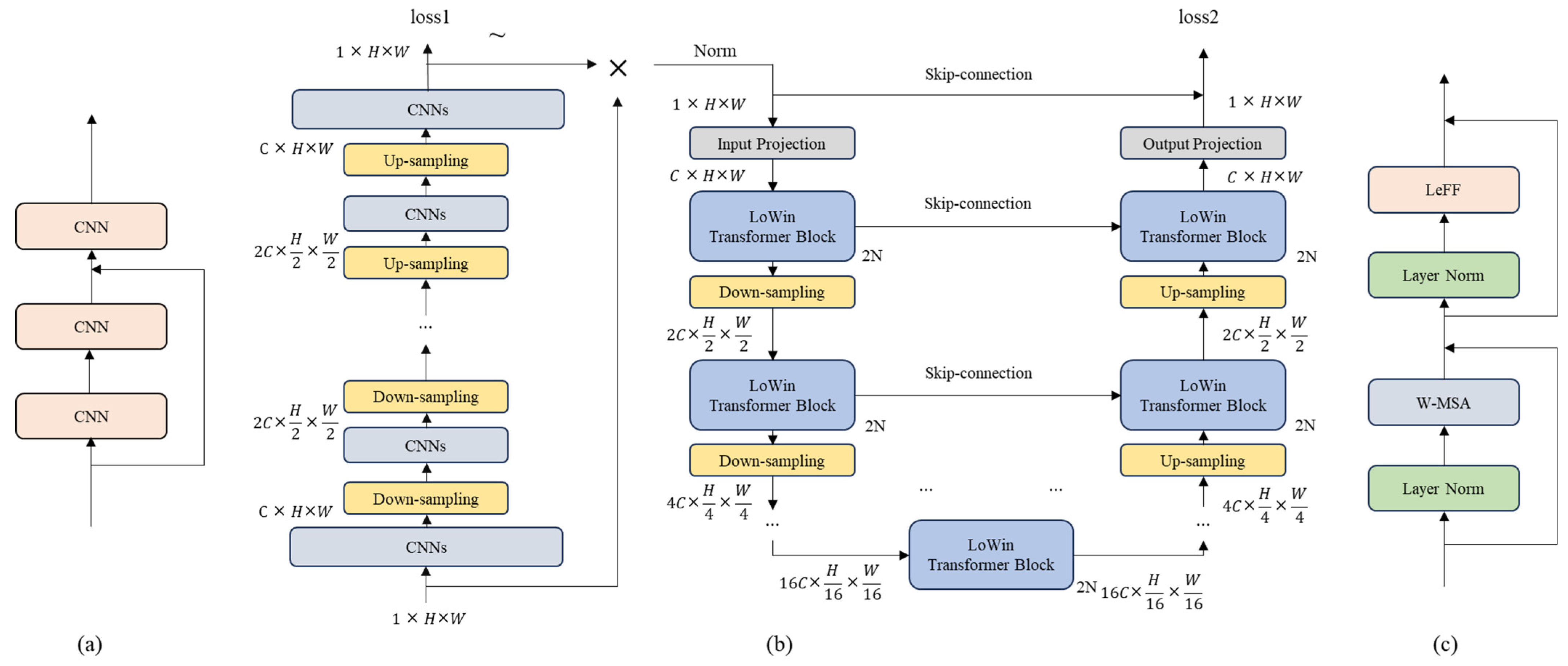
The proposed FuSINet is illustrated in Figure 5, Figure 5a is the structure of CNNs, Figure 5b shows the overall network diagram, and Figure 5b depicts the LoWin Transformer block. In Figure 5b, the network consists of two parts. The first part is a cascaded CNN, and the second part is a Uformer network. The first part only requires segmenting the interfered region, so we only built a simple CNN-based network. The second part aims to repair the image, so we built a Uformer network.

The network is constructed by fusing a segment and inpainting a network. In the first part, the network consists of an encoder and a decoder, both composed of multiple CNN layers. Each encoder layer reduces the image size and increases the number of channels, while each decoder layer increases the image size and decreases the number of channels.

In the first part, the encoder consists of L encoding layers, each encoding layer is composed of CNNs and a down-sampling layer, and the down-sampling layer reduces the length and width of the input data by half while doubling the number of channels. Each encoding layer can be represented as follows:

$$E_l=\mathrm{Down}-\mathrm{Sampling}\left(\mathrm{CNNs}\left({\mathrm{E}}_{l-1}\right)\right),$$

(14)

The decoder consists of L decoding layers. Each decoding layer is composed of an up-sampling layer and CNNs. The up-sampling layer, composed of convolutional layers, increases the feature resolution while reducing the number of channels. Each decoding layer can be represented as follows:

$$D_l=\mathrm{CNNs}\left(\mathrm{Up}-\mathrm{Sampling}\left(D_{l-1}\right)\right),$$

(15)

In the second part, like all autoencoders, the Uformer consists of an encoder and a decode, and skip connections are added between the encoder and decoder because the skip connections often show good performance in low-dimensional visual tasks. Additionally, two layers of LoWin Transformer blocks are added at the bottom of the U-shaped structure to further extract information and capture longer-range dependencies. In FuSINet, the input of the second part network consists of two parts. The first part is the raw input, and the second part is the output of the first part network. In this case, the input of the second part network can be represented as follows:

$$X_0=Norm\left(X-\left(H_{1}X\right)X\right),$$

(16)

where $Norm$ is the regularization function, $H_1$ is the matrix of the first stage network, and $X$ is the raw input.

The encoder consists of an input projection layer and L encoding layers. Each encoding layer is composed of 2N LoWin Transformer blocks and a down-sampling layer. The input projection layer is composed of convolutional layers and is responsible for extracting low-level features, denoted as $X_0\in R^{C\times H\times W}$, where C represents the number of channels. The two LoWin Transformer blocks within an encoding layer are designed by shift-windows to achieve global interaction, as shown in Figure 6. The down-sampling layer reduces the length and width of the input data by half while doubling the number of channels to increase the receptive field. Due to the reduction in image size, a larger field of view can be felt under the same patch. Given an input $X_0\in R^{C\times H\times W}$, the output feature map of the l-th encoding layer can be represented as $X_l\in R^{2^{l}C\times \frac{H}{2^k}\times \frac{W}{2^k}}$. Each encoding layer can be represented as follows:

$$E_l=\mathrm{Down}-\mathrm{Sampling}\left(\mathrm{LoWin}-\mathrm{Transformer}{\left({\mathrm{E}}_{l-1}\right)}_{2N}\right),$$

(17)

The decoder consists of an output projection layer and L decoding layers. Each decoding layer is composed of an up-sampling layer and 2N LoWin Transformer blocks. The up-sampling layer, composed of convolutional layers, increases the feature resolution while reducing the number of channels. The up-sampling features, along with the features from the corresponding encoding layer, are passed through the LoWin Transformer block. After L decoding layers, the features obtained by the decoder are restored to the original image by an output projection layer. Each decoding layer can be represented as follows:

$$D_l=\mathrm{LoWin}-\mathrm{Transformer}{\left(\mathrm{Up}-\mathrm{Sampling}\left(D_{l-1}\right)+E_l\right)}_{2N},$$

(18)

The proposed local attention windows have limited receptive fields, so in order to increase the receptive field, a double-layer LoWin Transformer block is employed, and the shift-windows between the two LoWin Transformer blocks are shown in Figure 6. The first layer represents the receptive field of the first LoWin Transformer block, where each differently colored block represents an attention window. The second layer represents the receptive field of the second LoWin Transformer block. Compared to the first layer, the second layer shifts the entire image by half of the window length along both dimensions. As a result, a single window in the second layer contains all four colors from the first layer, meaning the second layer’s receptive field includes all four independent regions from the first layer. Theoretically, with these two layers of LoWin Transformer blocks, global information interaction can be achieved.

The LoWin Transformer Block consists of W-MSA (Window-based Multi-head Self-Attention) and FFN (Feed-Forward Network). This module has the following advantages: 1. Compared to the standard Transformer, it significantly reduces computational costs. The standard Transformer computes global self-attention across the entire image, resulting in high computational costs. In contrast, the proposed method uses non-overlapping local window attention modules, which greatly reduces the computational costs. 2. This module can better capture both global and local information. W-MSA captures long-range information, while FFN captures local information.

The LoWin Transformer module can be represented as follows:

$$X_l^{\prime }=\mathrm{W}-\mathrm{MSA}\left(\mathrm{LN}\left(X_{l-1}\right)\right)+X_{l-1},$$

(19)

$$X_l=\mathrm{FFN}\left(\mathrm{LN}\left(X_l^{\prime }\right)\right)+X_l^{\prime },$$

(20)

Unlike the global self-attention in the standard Transformer, the non-overlapping local window self-attention mechanism efficiently reduces computational complexity. We first split $X\in R^{C\times H\times W}$ into non-overlapping blocks of size M × M, resulting in the input to W-MSA as $X^i\in R^{C\times M\times M}$. Next, we perform self-attention operations on each window. The computation process of the k-th head can be described as follows:

$$X=\left\{X^1,X^2,\cdots ,X^N\right\},N=HW/M^2,$$

(21)

$$Y_k^i=Attention\left(X^i{W}_k^Q,X^i{W}_k^K,X^i{W}_k^V\right),i=1,\cdots ,N,$$

(22)

$${\widehat{Y}}_k=\left\{Y_k^1,Y_k^2,\cdots ,Y_k^1\right\},$$

(23)

All the results of the heads are concatenated and linearly projected to obtain the final result. Inspired by the Swin Transformer, we also introduce relative position encoding B in the attention module. Therefore, the attention calculation process can be represented as follows:

$$Attention(Q,K,V)=Soft\max \left(\frac{Q{K}^T}{\sqrt{d_k}}+B\right)V,$$

(24)

Compared to global self-attention, the computational complexity of a single W-MSA is reduced from $O\left(H^2{W}^{2}C\right)$ to $O\left(M^{2}HWC\right)$, where M is the window size, which is generally much smaller than H and W. Since this network contains a large number of multi-head W-MSA blocks, the final computational complexity is significantly reduced.

The standard Transformer has limited capability to capture local contextual information. Considering the importance of neighboring pixels in image tasks, to further enhance the capture of local information, we add a feed-forward network (FFN) after W-SMA. The FFN consists of three convolutional layers.

3.4. Loss Function

The loss function consists of two parts, and the first part is as follows:

$$los{s}_1=\sqrt{{\left(H_{1}X-Y_1\right)}^2+{\epsilon }_1},$$

(25)

$$Y_1=\{\begin{array}{c}1,X_{pixel}\in RFI\\ 0,X_{pixel}\notin RFI\end{array},$$

(26)

The second part is as follows:

$$los{s}_2=\sqrt{{\left(H_2\cdot Norm\left(~\left(H_{1}X\right)\cdot X\right)-Y_2\right)}^2+{\epsilon }_2},$$

(27)

The final loss function is as follows:

$$loss=\alpha \cdot los{s}_1+\left(1-\alpha \right)\cdot los{s}_2,$$

(28)

$H_1$ is the matrix of the first stage network; $X$ is the input; $Y_1$ is the label of the first stage network; $H_2$ is the matrix of the second stage network; $Y_2$ is the label of the second stage network; ${\epsilon }_1$, ${\epsilon }_2$, and $\alpha$ are hyper-parameters. In this experiment, we set $\alpha =0.5$.

4. Experiments

In this section, three sets of experiments are conducted. The first set is ablation experiments, and this test set is the most complex, with randomly varying intensity and frequency of interference signal. This set aims to evaluate the performance of the proposed method. The second set is from MiniSAR with an imaging resolution of 0.1 m × 0.1 m, and the interference patterns include narrowband interference, chirp modulated wideband interference, and sinusoidal modulated wideband interference. This set aims to verify the effectiveness of the proposed algorithm on the three types of interference patterns. The third set is from the European Sentinel satellite with an imaging resolution of 3 m × 14 m. This set aims to demonstrate the performance of the proposed method on satellite data.

The network parameters are set as follows: we use the AdamW optimizer with momentum parameters (0.9, 0.999), weight decay exponent of 0.02, and initial learning rate of 2 × 10⁻⁴. The window size in LoWin Transformer is set to 8 × 8. Both the encoder and decoder have four layers. In W-MSA, the number of heads is 8. Two variants of the proposed network are provided in this paper: FuSINet (C = 16) and FuSINet-L (C = 32). The depth of the encoder and decoder is {2, 2, 2, 2}.

To quantitatively evaluate the experimental results, we use PSNR, SSIM, AG [37], and ME [30] as image quality assessment metrics. According to SAR characteristics, all input/output data are single-channel data with a size of 512 × 512 × 1. The data normalization is defined as follows:

$$\begin{array}{l}s=\frac{s-\min \left(s\right)}{\max \left(s\right)-\min \left(s\right)}\approx \frac{s}{\max \left(s\right)}\\ st.\max \left(s\right)>>\min \left(s\right)\end{array},$$

(29)

The mean entropy (ME) is defined as follows:

$$\mathrm{ME}=E\left(s\right)\cdot \mathrm{Entropy}\left(s\right),$$

(30)

The average gradient (AG) is defined as follows:

$$\mathrm{AG}=\frac{1}{\left(\mathrm{M}-1\right)\left(\mathrm{N}-1\right)}{\displaystyle {\sum }_{i=1}^{\mathrm{M}-1}{\displaystyle {\sum }_{j=1}^{\mathrm{N}-1}\sqrt{\frac{{\left(s\left(i+1,j\right)-s\left(i,j\right)\right)}^2+{\left(s\left(i,j+1\right)-s\left(i,j\right)\right)}^2}{2}}}}$$

(31)

A smaller mean value indicates that most of the interference has been eliminated, and a smaller entropy value indicates better image quality, so a smaller ME, a better performance, and a smaller AG indicates that the image is smoother.

4.1. Ablation Experiments

The parameters of RFI are shown in

Table 1. Interference parameters in ablation experiments.

Parameters	Value
Interference mode	Chirp
Radar bandwidth	150 MHz
Interference bandwidth	30 MHz~150 MHz
SIR	−20 dB~0 dB
Interference source	4

, and the interference pattern is chirp-modulated wideband interference. According to Equation (2), under the chirp-modulated wideband interference, the interference signal contains two variable parameters: the interference bandwidth and the interference power. The interference bandwidth randomly varies from 30 MHz to 150 MHz, and the signal-to-interference ratio (SIR) randomly varies from −20 dB to 0 dB. The proposed method is carried out in two stages. In the first stage, a segmentation network is used to remove RFI. In the second stage, an image restoration network is used to restore the clean image. The proposed algorithm [37], which directly restores the clean image from the interfered image, is referred to as the one-stage image restoration network. In the one-stage restoration network, due to variable interference power, the network needs more parameters to fit the changing values. In contrast, in the two-stage restoration algorithm, the highly perturbed components have been removed, making the network less sensitive to fluctuations in interference power. Therefore, theoretically, the proposed two-stage network holds better performance.

4.1.1. Time-Frequency Inpainting

The restored time-frequency maps are shown in Figure 7, and the performance metrics are shown in

Table 2. Performance indicators of repaired time-frequency maps.

Parameters	Algorithm	Size	PSNR/dB	SSIM
Non-parametric methods	DIFNet [56]	/	20.83 ± 0.05	/
One-stage Restoration Network	UNet [36]	28 M	28.16 ± 0.02	94.45%
	PISNet+ [37]	28 M	28.82 ± 0.03	94.81%
	Uformer	16 M	31.31 ± 0.02	96.32%
Two-stage Restoration Network	FuSINet	32 M	35.47 ± 0.03	98.12%
	FuSINet-L	72 M	36.22 ± 0.03	98.52%

. The compared methods can be roughly divided into three groups: non-parameterized methods, one-stage image restoration network, and two-stage image restoration network. The non-parameterized methods directly remove the interference from the time-frequency map without any restoration, resulting in the worst performance. In the one-stage image restoration network, the first two methods are CNN-based networks. To make a fair comparison, Dncnn in [36] is replaced by UNet. And the backbone CNN in PISNet [37] is replaced by UNet, referred to as PISNet+. The third method is the proposed Uformer. In the two-stage image restoration network, two model sizes are provided: FuSINet with fewer parameters and FuSINet-L with larger parameters.

Comparing UNet and Uformer, it can be observed that the Transformer-based network achieves significantly better performance than the CNN-based network. The Uformer improves PSNR by 3.15 dB and SSIM by 1.87% compared to UNet. Referring to Figure 7a, since radar signals and interference signals are wideband signals, the relationship between frequency and time is linear, indicating global characteristics. Therefore, the Transformer network, which is capable of capturing global features, performs better. Comparing the one-stage image restoration networks with the two-stage image restoration networks, it can be observed that, with the same parameters, the two-stage restoration network achieves a PSNR improvement of 4.16 dB and an SSIM improvement of 1.8% because the two-stage network has a simpler data distribution, resulting in better performance. Ultimately, the FuSINet-L with larger parameters achieves a PSNR of 36.22 dB and an SSIM of 98.52%.

4.1.2. SAR Image Inpainting

The results of SAR image inpainting are shown in Figure 8, and the performance metrics are shown in

Table 3. Performance indicators.

Parameters	Performance
	PSNR	SSIM
DIFNet [56]	23.01	67.06%
UNet [36]	27.12	83.90%
PISNet+ [37]	27.22	83.95%
Uformer	29.61	89.62%
FuSINet	34.00	95.69%
FuSINet-L	34.21	95.55%

. Referring to Table 3, compared to PISNet+, the proposed Uformer improves PSNR by 2.39 dB and SSIM by 5.67%. Compared to Uformer, the final proposed FuSINet achieves a PSNR improvement of 4.39 dB and an SSIM improvement of 6.07%. The larger-parameter version, FuSINet-L, achieves similar performance to FuSINet, indicating that larger network models do not significantly improve performance.

4.2. MiniSAR Data

In general, common RFI can be roughly divided into three categories: narrowband interference, chirp-modulated broadband interference, and sinusoidal-modulated broadband interference. This article conducts relevant experiments on these three types of interference, and the interference parameters are shown in

Table 4. Interference parameters in MiniSAR.

Parameters	Narrowband	Chirp	Sinusoidal
Interference bandwidth	<10 MHz	30 MHz~150 MHz	30 MHz~100 MHz
SIR	−15 dB~0 dB	−15 dB~0 dB	−15 dB~0 dB
Interference source	2	4	1

. In this chapter, PISNet+, Uformer, and FuSINet are used as comparative methods.

The time-frequency diagram of the narrowband interference is shown in Figure 9a, which contains two interference sources corresponding to the two straight lines. The test results of narrowband interference are shown in Figure 9 and Figure 10, where Figure 9 represents the restored time-frequency diagrams and Figure 10 represents the restored SAR images. The performance indicators for image restoration are shown in

Table 5. The performance indicators under single frequency interference.

Algorithm	Time-Frequency Map		SAR Image
	PSNR	SSIM	PSNR	PSNR
PISNet+	29.21	96.38%	28.49	88.82%
Uformer	32.71	96.21%	30.25	93.45%
FuSINet	34.20	97.88%	32.04	94.09%

. In the restored time-frequency map, compared to PISNet+, Uformer shows a PSNR improvement of 3.5 dB. Compared to Uformer, FuSINet exhibits a PSNR improvement of 1.49 dB, and the SSIM values of the three methods are relatively close. In the restored SAR image, compared to PISNet+, Uformer demonstrates a PSNR improvement of 1.76 dB and an SSIM improvement of 4.65%. Compared to Uformer, FuSINet shows a PSNR improvement of 1.79 dB, and the SSIM values are relatively close.

The time-frequency map of chirp-modulated broadband interference in MiniSAR is shown in Figure 11a, which includes four interference sources corresponding to the four diagonal lines. The test results of chirp broadband interference are shown in Figure 11 and Figure 12, where Figure 11 represents the restored time-frequency map, and Figure 12 represents the restored SAR image. The performance indicators for image restoration are shown in

Table 6. The performance indicators under chirp interference.

Algorithm	Time-Frequency Map		SAR Image
	PSNR	SSIM	PSNR	PSNR
PISNet+	27.13	94.59%	27.66	86.62%
Uformer	29.55	94.24%	29.44	90.59%
FuSINet	35.89	98.23%	34.59	96.48%

. In the restored time-frequency diagram, compared to PISNet+, Uformer shows a PSNR improvement of 2.42 dB and a similar SSIM value. Compared to Uformer, FuSINet exhibits a PSNR improvement of 6.34 dB and an SSIM improvement of 3.99%. In the restored SAR image, compared to PISNet+, Uformer demonstrates a PSNR improvement of 1.78 dB and an SSIM improvement of 3.97%. Compared to Uformer, FuSINet shows a PSNR improvement of 5.15 dB and an SSIM improvement of 5.89%.

The time-frequency map of the sinusoidal wideband interference in MiniSAR is shown in Figure 13a, which contains one interference source corresponding to a sinusoidal curve. The interference parameters are shown in Table 4, the interference bandwidth is 30 M~100 M, and the signal-to-interference ratio is −15 dB~0 dB. The results of the restoration are shown in Figure 13 and Figure 14, where Figure 13 shows the restored time-frequency map and Figure 14 shows the restored SAR image. The image restoration performance metrics are shown in

Table 7. The performance indicators under chirp interference.

Algorithm	Time-Frequency Map		SAR Image
	PSNR	SSIM	PSNR	PSNR
PISNet+	30.73	97.04%	29.88	91.31%
Uformer	35.18	97.07%	33.77	94.64%
FuSINet	37.09	98.27%	35.02	96.78%

. In the restored time-frequency map, compared to PISNet+, Uformer achieves a PSNR improvement of 4.45 dB and a similar SSIM value. Compared to Uformer, FuSINet achieves a PSNR improvement of 1.91 dB and an SSIM improvement of 1.2%. In the restored SAR image, compared to PISNet+, Uformer achieves a PSNR improvement of 3.89 dB and an SSIM improvement of 3.33%. Compared to Uformer, FuSINet achieves a PSNR improvement of 1.25 dB and an SSIM improvement of 2.14%.

Based on the above experiments, it can be concluded that among the three interference patterns, the proposed Robust Uformer performs exceptionally well and is relatively stable, while the one-stage algorithm is more significantly influenced by the interference patterns and intensity. So, the proposed FuSINet exhibits better robustness and performance.

4.3. Satellite Data

To verify the effectiveness of the proposed method on satellite data, the interfered image selected for the experiment is the third scene image shown in Figure 1, which is from the Sentinel-1 satellite, captured in February 2019 in South Korea. In this image, the interfered region contains rich targets and the intensity of the interfered region is high, making it suitable for testing. The time-frequency map of the interfered region is shown in Figure 15a, indicating that the interference is chirp-modulated wideband interference. The DIFNet, PISNet+, and FuSINet are selected as the compared methods. The restored time-frequency maps are shown in Figure 15, and the restored SAR images are shown in Figure 16 and Figure 17, with Figure 17 showing a close-up of the interfered region from Figure 16. It can be observed from Figure 16 and Figure 17 that most of the interference has been effectively filtered out. Under the same training data conditions, the proposed FuSINet achieves a better result, retains more targets compared to DIFNet, and has a cleaner interference removal effect compared to PISNet+.

In satellite data, we do not have interference data and clean data from the same region, so PSNR and SSIM metrics are no longer applicable. Instead, AG and ME are selected as image evaluation metrics. ME is equal to the product of the image mean and the image entropy. Theoretically, the lower the interference power, the smaller the image mean and image entropy, indicating better image quality. Therefore, ME can partially evaluate the effectiveness of interference suppression. However, when most of the targets are filtered out, the ME value will further decrease, so ME can only be used for approximate evaluation. In

Table 8. Performance indicators on Sentinel-1.

Algorithm	ME	AG
RFI data	3.35	1062
DIFNet	2.55	1127
PISNet+	2.65	1132
FuSINet	2.55	1110

, DIFNet loses more targets, resulting in a smaller ME value. Comparing Figure 15c,d, it can be seen that the FuSINet achieves a better image, with a decrease of 0.10 in ME. The AG metric represents image smoothness, where a lower value indicates better image quality. However, in interfered SAR images, the interfered region tends to be relatively homogeneous, while the targets exhibit more fluctuations due to the lower resolution of Sentinel-1. Therefore, the interfered image obtains the lowest AG value. In the filtered images, interference is theoretically eliminated, so a lower AG value indicates a smoother image. Compared to PISNet+, the FuSINet achieves better image restoration, with a decrease of 22 in AG.

5. Conclusions

SAR is a high-resolution imaging radar, and with an increase in carrier frequency, the imaging resolution of SAR can even reach the centimeter level, providing significant military and civilian value. However, SAR also faces complex electromagnetic interference. As a common interference pattern, RFI holds a high interference intensity and a wide coverage. For example, in Sentinel-1, the interfered region is generally larger than 30 square kilometers (0.5 M pixels). Additionally, compared to CV images, SAR images have lower information redundancy, making it challenging for traditional CV algorithms to restore SAR images. To address these issues, this paper proposes a robust time-frequency interference suppression method by fusing a segment and inpainting a network. And the FuSINet is embedded into the SAR imaging process. Compared to existing methods, the proposed method holds great improvements. First, the proposed global attention mechanism is more capable of capturing global features, resulting in significantly improved performance. Among them, the improvement of the receptive field is mainly achieved through Transformer, shift-windows, and down-sampling layers. Second, this article reconstructs the network structure to remove interference, resulting in better image restoration quality in the second stage. Since the currently deployed SAR satellites usually do not hold system-level anti-interference capabilities, our proposed method can liberate clean images from the interfered images, thereby preventing satellites from being blinded by interference. However, due to modeling limitations, the theory analysis and experiments of this paper did not cover complex interference patterns such as compound RFI. We leave this for future studies.

References

1. Zhu, X.X.; Bamler, R. Very High Resolution Spaceborne SAR Tomography in Urban Environment. IEEE Trans. Geosci. Remote Sens. 2010, 48, 4296–4308. [Google Scholar] [CrossRef]
2. Pu, W. Deep SAR Imaging and Motion Compensation. IEEE Trans. Image Process. 2021, 30, 2232–2247. [Google Scholar] [CrossRef]
3. Hou, X.; Ao, W.; Song, Q.; Lai, J.; Wang, H.; Xu, F. FUSAR-Ship: Building a high-resolution SAR-AIS matchup dataset of Gaofen-3 for ship detection and recognition. Sci. China-Inf. Sci. 2020, 63, 140303. [Google Scholar] [CrossRef]
4. Adeli, S.; Salehi, B.; Mahdianpari, M.; Quackenbush, L.J.; Brisco, B.; Tamiminia, H.; Shaw, S. Wetland Monitoring Using SAR Data: A Meta-Analysis and Comprehensive Review. Remote Sens. 2020, 12, 2190. [Google Scholar] [CrossRef]
5. Tebaldini, S.; Manzoni, M.; Tagliaferri, D.; Rizzi, M.; Monti-Guarnieri, A.V.; Prati, C.M.; Spagnolini, U.; Nicoli, M.; Russo, I.; Mazzucco, C. Sensing the Urban Environment by Automotive SAR Imaging: Potentials and Challenges. Remote Sens. 2022, 14, 3602. [Google Scholar] [CrossRef]
6. Li, M.-D.; Cui, X.-C.; Chen, S.-W. Adaptive Superpixel-Level CFAR Detector for SAR Inshore Dense Ship Detection. IEEE Geosci. Remote Sens. Lett. 2021, 19, 4010405. [Google Scholar] [CrossRef]
7. Li, N.; Lv, Z.; Guo, Z.; Zhao, J. Time-Domain Notch Filtering Method for Pulse RFI Mitigation in Synthetic Aperture Radar. IEEE Geosci. Remote Sens. Lett. 2021, 19, 4013805. [Google Scholar] [CrossRef]
8. Cai, Y.; Li, J.; Yang, Q.; Liang, D.; Liu, K.; Zhang, H.; Lu, P.; Wang, R. First Demonstration of RFI Mitigation in the Phase Synchronization of LT-1 Bistatic SAR. IEEE Trans. Geosci. Remote Sens. 2023, 61, 5217319. [Google Scholar] [CrossRef]
9. Yang, H.; He, Y.; Du, Y.; Zhang, T.; Yin, J.; Yang, J. Two-Dimensional Spectral Analysis Filter for Removal of LFM Radar Interference in Spaceborne SAR Imagery. IEEE Trans. Geosci. Remote Sens. 2021, 60, 5219016. [Google Scholar] [CrossRef]
10. Tao, M.; Su, J.; Huang, Y.; Wang, L. Mitigation of Radio Frequency Interference in Synthetic Aperture Radar Data: Current Status and Future Trends. Remote Sens. 2019, 11, 2438. [Google Scholar] [CrossRef]
11. Zhou, F.; Wu, R.; Xing, M.; Bao, Z. Eigensubspace-based filtering with application in narrow-band interference suppression for SAR. IEEE Geosci. Remote Sens. Lett. 2007, 4, 75–79. [Google Scholar] [CrossRef]
12. Yang, H.; Li, K.; Li, J.; Du, Y.; Yang, J. BSF: Block Subspace Filter for Removing Narrowband and Wideband Radio Interference Artifacts in Single-Look Complex SAR Images. IEEE Trans. Geosci. Remote Sens. 2022, 60, 5211916. [Google Scholar] [CrossRef]
13. Zhou, F.; Tao, M.; Bai, X.; Liu, J. Narrow-Band Interference Suppression for SAR Based on Independent Component Analysis. IEEE Trans. Geosci. Remote Sens. 2013, 51, 4952–4960. [Google Scholar] [CrossRef]
14. Buckreuss, S.; Horn, R. E-SAR P-band SAR subsystem design and RF-interference suppression. In Proceedings of the IGARSS ‘98. Sensing and Managing the Environment, 1998 IEEE International Geoscience and Remote Sensing, Symposium Proceedings, (Cat. No.98CH36174), Seattle, WA, USA, 6–10 July 1998; Volume 1, pp. 466–468. [Google Scholar]
15. Cazzaniga, G.; Guarnieri, A.M. Removing RF interferences from P-band airplane SAR data. In Proceedings of the IGARSS ‘96. 1996 International Geoscience and Remote Sensing Symposium, Lincoln, NE, USA, 31 May 1996; Volume 3, pp. 1845–1847. [Google Scholar]
16. Reigber, A.; Ferro-Famil, L. Interference suppression in synthesized SAR images. IEEE Geosci. Remote Sens. Lett. 2005, 2, 45–49. [Google Scholar] [CrossRef]
17. Xu, W.; Xing, W.; Fang, C.; Huang, P.; Tan, W. RFI Suppression Based on Linear Prediction in Synthetic Aperture Radar Data. IEEE Geosci. Remote Sens. Lett. 2020, 18, 2127–2131. [Google Scholar] [CrossRef]
18. Fu, Z.; Zhang, H.; Zhao, J.; Li, N.; Zheng, F. A Modified 2-D Notch Filter Based on Image Segmentation for RFI Mitigation in Synthetic Aperture Radar. Remote Sens. 2023, 15, 846. [Google Scholar] [CrossRef]
19. Yi, J.; Wan, X.; Cheng, F.; Gong, Z. Computationally Efficient RF Interference Suppression Method with Closed-Form Maximum Likelihood Estimator for HF Surface Wave Over-The-Horizon Radars. IEEE Trans. Geosci. Remote Sens. 2012, 51, 2361–2372. [Google Scholar] [CrossRef]
20. Shi, J.R.; Zhen, X.Y.; Wei, Z.T.; Yang, W. Survey on algorithms of low-rank matrix recovery. Appl. Res. Comput. 2013, 30, 1601–1605. [Google Scholar]
21. Nguyen, L.H.; Tran, T.; Do, T. Sparse Models and Sparse Recovery for Ultra-Wideband SAR Applications. IEEE Trans. Aerosp. Electron. Syst. 2014, 50, 940–958. [Google Scholar] [CrossRef]
22. Nguyen, L.H.; Tran, T.D. Efficient and Robust RFI Extraction Via Sparse Recovery. IEEE J. Sel. Top. Appl. Earth Obs. Remote Sens. 2016, 9, 2104–2117. [Google Scholar] [CrossRef]
23. Liu, H.; Li, D.; Zhou, Y.; Truong, T.-K. Joint Wideband Interference Suppression and SAR Signal Recovery Based on Sparse Representations. IEEE Geosci. Remote Sens. Lett. 2017, 14, 1542–1546. [Google Scholar] [CrossRef]
24. Liu, H.; Li, D.; Zhou, Y.; Truong, T.-K. Simultaneous Radio Frequency and Wideband Interference Suppression in SAR Signals via Sparsity Exploitation in Time-Frequency Domain. IEEE Trans. Geosci. Remote Sens. 2018, 56, 5780–5793. [Google Scholar] [CrossRef]
25. Su, J.; Tao, H.; Tao, M.; Wang, L.; Xie, J. Narrow-Band Interference Suppression via RPCA-Based Signal Separation in Time–Frequency Domain. IEEE J. Sel. Top. Appl. Earth Obs. Remote Sens. 2017, 10, 5016–5025. [Google Scholar] [CrossRef]
26. Tao, M.; Li, J.; Su, J.; Fan, Y.; Wang, L.; Zhang, Z. Interference Mitigation for Synthetic Aperture Radar Data using Tensor Representation and Low-Rank Approximation. In Proceedings of the 2020 33rd General Assembly and Scientific Symposium of the International Union of Radio Science, Rome, Italy, 29 August–5 September 2020. [Google Scholar]
27. Joy, S.; Nguyen, L.H.; Tran, T.D. Radio frequency interference suppression in ultra-wideband synthetic aperture radar using range-azimuth sparse and low-rank model. In Proceedings of the 2016 IEEE Radar Conference (RadarConf), Philadelphia, PA, USA, 2–6 May 2016; pp. 433–436. [Google Scholar]
28. Huang, Y.; Liao, G.; Li, J.; Xu, J. Narrowband RFI Suppression for SAR System via Fast Implementation of Joint Sparsity and Low-Rank Property. IEEE Trans. Geosci. Remote Sens. 2018, 56, 2748–2761. [Google Scholar] [CrossRef]
29. Lyu, Q.; Han, B.; Li, G.; Sun, W.; Pan, Z.; Hong, W.; Hu, Y. SAR interference suppression algorithm based on low-rank and sparse matrix decomposition in time–frequency domain. IEEE Geosci. Remote Sens. Lett. 2021, 19, 4008305. [Google Scholar] [CrossRef]
30. Huang, Y.; Zhang, L.; Yang, X.; Chen, Z.; Liu, J.; Li, J.; Hong, W. An Efficient Graph-Based Algorithm for Time-Varying Narrowband Interference Suppression on SAR System. IEEE Trans. Geosci. Remote Sens. 2021, 59, 8418–8432. [Google Scholar] [CrossRef]
31. Huang, Y.; Wen, C.; Chen, Z.; Chen, J.; Liu, Y.; Li, J.; Hong, W. HRWS SAR Narrowband Interference Mitigation Using Low-Rank Recovery and Image-Domain Sparse Regularization. IEEE Trans. Geosci. Remote Sens. 2021, 60, 5217914. [Google Scholar] [CrossRef]
32. Huang, Y.; Zhang, L.; Li, J.; Hong, W.; Nehorai, A. A Novel Tensor Technique for Simultaneous Narrowband and Wideband Interference Suppression on Single-Channel SAR System. IEEE Trans. Geosci. Remote Sens. 2019, 57, 9575–9588. [Google Scholar] [CrossRef]
33. Chen, S.; Lin, Y.; Yuan, Y.; Li, X.; Hou, L.; Zhang, S. Suppressive Interference Suppression for Airborne SAR Using BSS for Singular Value and Eigenvalue Decomposition Based on Information Entropy. IEEE Trans. Geosci. Remote Sens. 2023, 61, 5205611. [Google Scholar] [CrossRef]
34. Wei, S.; Zhang, H.; Zeng, X.; Zhou, Z.; Shi, J.; Zhang, X. CARNet: An effective method for SAR image interference suppression. Int. J. Appl. Earth Obs. Geoinf. 2022, 114, 103019–103026. [Google Scholar] [CrossRef]
35. Li, X.; Ran, J.; Zhang, H. ISRNet: An Effective Network for SAR Interference Suppression and Recognition. In Proceedings of the 2022 IEEE 9th International Symposium on Microwave, Antenna, Propagation and EMC Technologies for Wireless Communications (MAPE), Chengdu, China, 26–29 August 2022; pp. 428–431. [Google Scholar]
36. Fan, W.; Zhou, F.; Tao, M.; Bai, X.; Rong, P.; Yang, S.; Tian, T. Interference Mitigation for Synthetic Aperture Radar Based on Deep Residual Network. Remote Sens. 2019, 11, 1654. [Google Scholar] [CrossRef]
37. Shen, J.; Han, B.; Pan, Z.; Li, G.; Hu, Y.; Ding, C. Learning Time–Frequency Information With Prior for SAR Radio Frequency Interference Suppression. IEEE Trans. Geosci. Remote Sens. 2022, 60, 5239716. [Google Scholar] [CrossRef]
38. Dong, L.; Yang, N.; Wang, W.; Wei, F.; Liu, X.; Wang, Y.; Gao, J.; Zhou, M.; Hon, H.W. Unified language model pre-training for natural language understanding and generation. In Proceedings of the 33rd International Conference on Neural Information Processing Systems, Vancouver, BC, Canada, 8–14 December 2019; pp. 13063–13075. [Google Scholar]
39. Radford, A.; Wu, J.; Child, R.; Luan, D.; Amodei, D.; Sutskever, I. Language models are unsupervised multitask learners. OpenAI Blog 2019, 1, 9. [Google Scholar]
40. Brown, T.; Mann, B.; Ryder, N.; Subbiah, M.; Kaplan, J.D.; Dhariwal, P.; Neelakantan, A.; Shyam, P.; Sastry, G.; Askell, A.; et al. Language models are few-shot learners. Adv. Neural Inf. Process. Syst. 2020, 33, 1877–1901. [Google Scholar]
41. Kocoń, J.; Cichecki, I.; Kaszyca, O.; Kochanek, M.; Szydło, D.; Baran, J.; Bielaniewicz, J.; Gruza, M.; Janz, A.; Kanclerz, K.; et al. ChatGPT: Jack of all trades, master of none. Inf. Fusion 2023, 99, 101861. [Google Scholar] [CrossRef]
42. Devlin, J.; Chang, M.-W.; Lee, K.; Toutanova, K.; Computat, L.A. BERT: Pre-training of Deep Bidirectional Transformers for Language Understanding. In Proceedings of the Conference of the North-American-Chapter of the Association-for-Computational-Linguistics-Human Language Technologies (NAACL-HLT), Minneapolis, MN, USA, 2–7 June 2019; pp. 4171–4186. [Google Scholar]
43. Liu, Y.; Ott, M.; Goyal, N.; Du, J.; Joshi, M.; Chen, D.; Levy, O.; Lewis, M.; Zettlemoyer, L.; Stoyanov, V. RoBERTa: A Robustly Optimized BERT Pretraining Approach. Inf. Syst. Res. 2019. [Google Scholar]
44. Dosovitskiy, A.; Beyer, L.; Kolesnikov, A.; Weissenborn, D.; Zhai, X.; Unterthiner, T.; Dehghani, M.; Minderer, M.; Heigold, G.; Gelly, S.; et al. An Image is Worth 16 × 16 Words: Transformers for Image Recognition at Scale. arXiv 2021, arXiv:2010.11929. [Google Scholar]
45. Han, K.; Wang, Y.; Chen, H.; Chen, X.; Guo, J.; Liu, Z.; Tang, Y.; Xiao, A.; Xu, C.; Xu, Y.; et al. A Survey on Vision Transformer. IEEE Trans. Pattern Anal. Mach. Intell. 2023, 45, 87–110. [Google Scholar] [CrossRef] [PubMed]
46. Wang, X.; Girshick, R.; Gupta, A.; He, K. Non-local Neural Networks. In Proceedings of the IEEE Conference on Computer Vision and Pattern Recognition (CVPR), Salt Lake City, UT, USA, 18–23 June 2018; Volume 2. [Google Scholar]
47. Hu, J.; Shen, L.; Sun, G. Squeeze-and-Excitation Networks. In Proceedings of the 2018 IEEE/CVF Conference on Computer Vision and Pattern Recognition, Salt Lake City, UT, USA, 18–23 June 2018; Volume 2. [Google Scholar]
48. Wang, Z.; Cun, X.; Bao, J.; Zhou, W.; Liu, J.; Li, H. Uformer: A general u-shaped transformer for image restoration. In Proceedings of the IEEE/CVF Conference on Computer Vision and Pattern Recognition, New Orleans, LA, USA, 18–24 June 2022; pp. 17683–17693. [Google Scholar]
49. He, K.; Chen, X.; Xie, S.; Li, Y.; Dollár, P.; Girshick, R. Masked autoencoders are scalable vision learners. In Proceedings of the IEEE/CVF Conference on Computer Vision and Pattern Recognition, New Orleans, LA, USA, 18–24 June 2022; pp. 16000–16009. [Google Scholar]
50. Heo, B.; Yun, S.; Han, D.; Chun, S.; Choe, J.; Oh, S.J. Rethinking Spatial Dimensions of Vision Transformers. In Proceedings of the 2021 IEEE/CVF International Conference on Computer Vision (ICCV), Montreal, QC, Canada, 10–17 October 2021. [Google Scholar]
51. Wang, W.; Xie, E.; Li, X.; Fan, D.-P.; Song, K.; Liang, D.; Lu, T.; Luo, P.; Shao, L. Pyramid Vision Transformer: A Versatile Backbone for Dense Prediction without Convolutions. In Proceedings of the 2021 IEEE/CVF International Conference on Computer Vision (ICCV), Montreal, QC, Canada, 10–17 October 2021. [Google Scholar]
52. Dong, X.; Bao, J.; Chen, D.; Zhang, W.; Yu, N.; Yuan, L.; Chen, D.; Guo, B. Cswin transformer: A general vision transformer backbone with cross-shaped windows. In Proceedings of the IEEE/CVF Conference on Computer Vision and Pattern Recognition, New Orleans, LA, USA, 18–24 June 2022; pp. 12124–12134. [Google Scholar]
53. Liu, Y.; Zhang, Y.; Wang, Y.; Hou, F.; Yuan, J.; Tian, J.; Zhang, Y.; Shi, Z.; Fan, J.; He, Z. A survey of visual transformers. IEEE Trans. Neural Netw. Learn. Syst. 2023, 1–21. [Google Scholar] [CrossRef] [PubMed]
54. Khan, S.; Naseer, M.; Hayat, M.; Zamir, S.W.; Khan, F.S.; Shah, M. Transformers in Vision: A Survey. ACM Comput. Surv. 2022, 54, 1–41. [Google Scholar] [CrossRef]
55. Li, H.; Wang, M.; Lu, S.; Wan, H.; Cui, X.; Chen, P.-Y. Transformers as Multi-Task Feature Selectors: Generalization Analysis of In-Context Learning. In Proceedings of the NeurIPS 2023 Workshop on Mathematics of Modern Machine Learning, New Orleans, LA, USA, 16 December 2023. [Google Scholar]
56. Fang, F.; Lv, W.; Dai, D. DIFNet: SAR RFI Suppression Based on domain invariant feartures. arXiv 2024, arXiv:2403.02894. [Google Scholar]
Figure 1. Common RFI in Sentinel-1 satellites.
Remotesensing 16 01013 g001
Figure 2. Algorithm performance diagram.
Remotesensing 16 01013 g002
Figure 3. Diagram of radio frequency interference.
Remotesensing 16 01013 g003
Figure 4. RFI suppression pipeline based on fusing segmentation and inpainting networks in the time-frequency domain.
Remotesensing 16 01013 g004
Figure 5. Network diagram: (a) CNNs; (b) FuSINet; (c) LoWin Transformer block.
Remotesensing 16 01013 g005
Figure 6. Receptive field of double-layer LoWin Transformer block.
Remotesensing 16 01013 g006
Figure 7. Restored time-frequency maps: (a) Jamming data; (b) Label; (c) DIFNet; (d) UNet; (e) PISNet+; (f) Uformer; (g) FuSINet; (h) FuSINet-L.
Remotesensing 16 01013 g007
Figure 8. SAR images: (a) Jamming data; (b) Label; (c) DIFNet; (d) UNet; (e) PISNet+; (f) Uformer; (g) FuSINet; (h) FuSINet-L.
Remotesensing 16 01013 g008
Figure 9. Time-frequency map under single frequency interference: (a) Jamming data; (b) Label; (c) PISNet+; (d) Uformer; (e) FuSINet.
Remotesensing 16 01013 g009
Figure 10. SAR image under single frequency interference: (a) Jamming data; (b) Label; (c) PISNet+; (d) Uformer; (e) FuSINet.
Remotesensing 16 01013 g010
Figure 11. Time-frequency map under chirp interference: (a) Jamming data; (b) Label; (c) PISNet+; (d) Uformer; (e) FuSINet.
Remotesensing 16 01013 g011
Figure 12. SAR image under chirp interference: (a) Jamming data; (b) Label; (c) PISNet+; (d) Uformer; (e) FuSINet.
Remotesensing 16 01013 g012
Figure 13. Time-frequency map under sinusoidal interference: (a) Jamming data; (b) Label; (c) PISNet+; (d) Uformer; (e) FuSINet.
Remotesensing 16 01013 g013
Figure 14. SAR image under sinusoidal interference: (a) Jamming data; (b) Label; (c) PISNet+; (d) Uformer; (e) FuSINet.
Remotesensing 16 01013 g014
Figure 15. The restored time-frequency diagram on Sentinel-1: (a) Jamming data; (b) DIFNet; (c) PISNet+; (d) FuSINet.
Remotesensing 16 01013 g015
Figure 16. The restored SAR image on Sentinel-1: (a) Jamming data, The red rectangular box indicates the location where the interference occurs; (b) DIFNet; (c) PISNet+; (d) FuSINet.
Remotesensing 16 01013 g016
Figure 17. The restored local SAR image on Sentinel-1: (a) Jamming data; (b) DIFNet; (c) PISNet+; (d) FuSINet.
Remotesensing 16 01013 g017