Abstract
The vertical profiles of aerosol optical properties are vital to clarify their transboundary transport, climate forcing and environmental health influences. Based on synergistic measurements of multiple advanced detection techniques, this study investigated aerosol vertical structure and optical characteristics during two dust and haze events in Lanzhou of northwest China. Dust particles originated from remote deserts traveled eastward at different altitudes and reached Lanzhou on 10 April 2020. The trans-regional aloft (~4.0 km) dust particles were entrained into the ground, and significantly modified aerosol optical properties over Lanzhou. The maximum aerosol extinction coefficient (σ), volumetric depolarization ratio (VDR), optical depth at 500 nm (AOD500), and surface PM10 and PM2.5 concentrations were 0.4~1.5 km−1, 0.15~0.30, 0.5~3.0, 200~590 μg/m3 and 134 μg/m3, respectively, under the heavy dust event, which were 3 to 11 times greater than those at the background level. The corresponding Ångström exponent (AE440–870), fine-mode fraction (FMF) and PM2.5/PM10 values consistently persisted within the ranges of 0.10 to 0.50, 0.20 to 0.50, and 0.20 to 0.50, respectively. These findings implied a prevailing dominance of coarse-mode and irregular non-spherical particles. A severe haze episode stemming from local emissions appeared at Lanzhou from 30 December 2020 to 2 January 2021. The low-altitude transboundary transport aerosols seriously deteriorated the air quality level in Lanzhou, and aerosol loading, surface air pollutants and fine-mode particles strikingly increased during the gradual strengthening of haze process. The maximum AOD500, AE440–870nm, FMF, PM2.5 and PM10 concentrations, and PM2.5/PM10 were 0.65, 1.50, 0.85, 110 μg/m3, 180 μg/m3 and 0.68 on 2 January 2021, respectively, while the corresponding σ and VDR at 0.20–0.80 km height were maintained at 0.68 km−1 and 0.03~0.12, implying that fine-mode and spherical small particles were predominant. The profile of ozone concentration exhibited a prominent two-layer structure (0.60–1.40 km and 0.10–0.30 km), and both concentrations at two heights always remained at high levels (60~72 μg/m3) during the entire haze event. Conversely, surface ozone concentration showed a significant decrease during severe haze period, with the peak value of 20~30 μg/m3, which was much smaller than that before haze pollution (~80 μg/m3 on 30 December). Our results also highlighted that the vertical profile of aerosol extinction coefficient was a good proxy for evaluating mass concentrations of surface particulate matters under uniform mixing layers, which was of great scientific significance for retrieving surface air pollutants in remote desert or ocean regions. These statistics of the aerosol vertical profiles and optical properties under heavy dust and haze events in Lanzhou would contribute to investigate and validate the transboundary transport and radiative forcing of aloft aerosols in the application of climate models or satellite remote sensing.
1. Introduction
Airborne aerosol particles play a crucial role in modulating the radiation energy budget balance of the Earth–atmosphere system [1,2,3] and altering cloud microphysical characteristics through diverse complex physical and chemical mechanisms [4,5,6], and thus exert a far-reaching influence on the regional precipitation pattern and climate change [3,7]. Aerosol optical properties and vertical profiles of the extinction coefficient are two key parameters for accurately evaluating their transboundary transport and climatic and environmental impacts [8,9,10]. Moreover, the ground-truth aerosol vertical distribution from Lidar was widely used to validate the retrievals of satellite-based aerosol products and projections of aerosol climate models.
To date, the scientific community has made numerous efforts to quantitatively explore aerosol vertical structures and assess their climate radiative forcing throughout the world. Liu et al. [11] presented a height-resolved global distribution of dust aerosols for the first time from Cloud-Aerosol Lidar Infrared Pathfinder Satellite (CALIPSO) lidar measurements, and indicated that global dust aerosol showed a significantly latitude and spatiotemporal distribution, and a strong seasonal cycle, which was primarily reliant on the desert source regions and prevailing atmospheric general circulation. Huang et al. [12] analyzed the vertical structures and long-range transport of dust aerosol observed by three micro-pulse lidar systems and suggested that the height of dust layer was mainly located at an altitude of 2–3 km in northwest China during spring 2008. These uplifted dust particles would travel easterly over long-range on a subcontinental scale, even across the Pacific Ocean, and produced remarkable shortwave and longwave radiative heating rates on atmospheric layer, eventually had an important influence on the dynamic and thermal structure of the atmosphere [1,13]. Sheng et al. [14] studied the aerosol vertical distribution and optical properties in different pollution events in Beijing during autumn 2017, and found that coarse-mode and irregular particles with a large linear depolarization ratio played a leading role during dust events, whereas the aerosols were dominant by highly spherical water soluble particles, weak light-scattering and small depolarization ratio during haze events. Sun et al. [15] examined the aerosol optical characteristics and vertical distributions under enhanced haze pollution events in Yangtze River Delta region during 2013–2015 by using micro-pulse lidar and sun-photometer observations and elucidated the effect of regional transport of different aerosol types over eastern China. Qin et al. [16] investigated several transboundary aloft transport events of haze aerosols to Xuzhou, eastern China, through a synergic approach and highlighted that the transported aloft aerosols led to the rapid formation of secondary inorganic substances, which strongly contributed to haze event formation. Huang et al. [17] provided observational evidences on aloft aerosol and planetary boundary layer (PBL) interaction and its impact on pollution aggravation. They revealed that aerosols could exert a significant heating in upper PBL and a substantial dimming near surface under enhanced haze pollution in Beijing. Therefore, a complete knowledge of aerosol vertical profile and optical properties is pivotal to ascertain their transboundary transport, environmental and climatic impacts on a regional scale.
Lanzhou, the capital city of Gansu province, is situated at the junction of Loess Plateau, Qinghai-Tibet Plateau, and Inner Mongolian Plateau, which is an important industrial base over northwest China. Petrochemical refinery, non-ferrous metal smelting, and manufacturing are heavily polluted industries and combustion of coal fuel is a major energy source in Lanzhou [18]. Lanzhou has once become one of the heaviest air-polluted cities in China before 2013. The earliest photochemical smog pollution event in China was found at Xigu district of Lanzhou in 1980s [19], which has attracted a considerable attention all over the world. In order to control the ambient air pollution in Lanzhou, the local government and environmental protection bureau have promulgated various stringent regulations and mitigation strategies since 2013. Consequently, the air quality of Lanzhou has been greatly improved and the so-called ‘Lanzhou Blue’ appeared frequently in recent decades. For instance, the total number of fine days with low concentrations of particulate matter (PM2.5 and PM10) and other gaseous precursors (SO2, NO2, CO, and O3) increased distinctly from 2013 to 2016 [20]. Hence, Lanzhou was awarded the Today’s Transformative Progress Award 2015 by the United Nations attributed to its significant improvement in urban air quality. However, the annual growth rate of motor vehicle was more than 80 thousand since 2010 with total amount exceeding 1.32 million at present, and it would unavoidably release massive automobile exhaust gas, eventually exacerbated air pollution level of the city. Zhao et al. [20,21] indicated that although the particulate matter pollution in Lanzhou has become very light in recent years, vehicle exhaust and ozone pollution was increasingly severe. Due to unique valley basin terrain, the calm weather and strong temperature inversion layer frequently appeared in Lanzhou during winter; thus, the air pollutants were usually trapped inside the basin [22]. The international media often reported that a gray and thick smog layer frequently hung over the urban area of Lanzhou during the domestic heating period, which was greatly harmful to public health.
Thus far, there have been a great number of studies focusing on particulate mass loading and ambient air pollutants in Lanzhou. Ta et al. [23] revealed that concentrations of gaseous and particulate pollutants in urban Lanzhou had an obvious seasonal variation, with a winter maximum for SO2 (90~210 μgm−3) and NO2 (70~90 μgm−3), and a spring maximum for total suspended particulate (890~1040 μgm−3). Chu et al. [22] analyzed SO2 pollution in Lanzhou metropolitan area utilizing air quality measurements of Air Pollution and Control in Lanzhou (APCL) project, and simulated diffusion and transport of SO2 using HYPACT regional model. They suggested that SO2 pollution in Lanzhou was largely dependent upon the emission source and stable stratification during daytime and nighttime. Wang et al. [18] sampled different size particulate matters (TSP, PM10, PM2.5 and PM1.0) in Lanzhou during 2005 and showed that the monthly average concentrations of coarse particles (TSP and PM10) were bimodal with the highest peak in April, while the annual distributions of fine particles (PM1.0 and PM2.5) were unimodal with the peak value in December. Wang et al. [24] implied that dust particles commonly mixed with local anthropogenic air pollutants at SACOL (a rural site of Lanzhou) during spring 2007, which might bring major uncertainties in quantification of regional climatic effect. Xu et al. [25] indicated that the mean chemical compositions of submicron particulate matter (PM1.0) consisted of 47% organics, 16% sulfate, 12% black carbon, 11% ammonium, 10% nitrate, and 4% chloride in urban Lanzhou during summertime of 2012, measuring by an Aerodyne high-resolution time-of-flight aerosol mass spectrometer (HR-ToF-AMS). In terms of aerosol optical characteristics and vertical profile, Bi et al. [26] and Che et al. [27] manifested that aerosol optical properties at suburban and urban Lanzhou showed a pronounced annual cycle, with maximum aerosol loading in spring or winter periods. Cao et al. [28] revealed that the aerosol extinction coefficient at SACOL was mostly located below a height of 3 km and decreased with height from November 2010 to February 2011. Zhao et al. [29] studied a dust event that occurred at Lanzhou during 9–14 March 2013, and identified sources of the dust based on CALIPSO, MODIS satellite data and a backward trajectory model. Nevertheless, the previous studies mainly focused on the daytime variations in aerosol optical properties, and the knowledge on nighttime aerosol optical features and its vertical profiles in Lanzhou still remain insufficient, which restrains our understanding of the influences of aerosol on transboundary transport and regional climate change.
To this end, this study investigated the diurnal variations of aerosol vertical profiles and optical properties in Lanzhou during two dust and haze episodes and quantitatively evaluated the relative contributions of the trans-regional transport of aloft aerosols advected into urban Lanzhou. We mainly analyzed the vertical structures of the aerosol extinction coefficient, particle linear depolarization ratio, and ozone concentration, spectral aerosol optical depth, Ångström exponent (440–870 nm), fine-mode fraction, and mass concentrations of six air pollutants (PM2.5, PM10, SO2, NO2, CO and O3) and explored the potential sources of dust and haze aerosols, combined with ground-based synergistic observations and backward trajectory model. The structure of this article is organized as follows. Section 2 introduces site information and instruments. Section 3 presents the retrieval methods and methodology and Section 4 shows the results analysis and discussion. The primary findings and Summary are given in Section 5.
2. Site Description and Measurement
2.1. Site Information
Lanzhou site (36.047°N, 103.854°E, 1621 m above m.s.l.) is located at the southeastern urban area of Lanzhou (i.e., Chengguan district). A new CE318-T photometer was set up on the rooftop of a 22-floor Guanyun building (about 100 m above ground) in the main campus of Lanzhou University in December 2019. The Chengguan district is a metropolitan area and comprises governmental, commercial, cultural, and residential elements [22]. The topography of Lanzhou is characterized by a narrow north–south-oriented (2~8 km) and long northwest–southeast-oriented (about 35 km) valley basin along Yellow River. The total urban area covers 13,085.6 km2, including five municipal districts, and the residential population is nearly 4.40 million. The climatic pattern of this region belongs to typical temperate continental semiarid climate with four distinct seasons. The annual average temperature and precipitation here are 10.3 °C and 327.8 mm, respectively, concentrated from June to September, whereas the total annual evaporation is as high as 1437 mm. Annual mean wind speed is 1.2 m/s and the frequency of calm wind is about 60% with more than 82% for winter. Due to its special trough-shaped topography of valley basin and climatic condition, the thermal inversion of atmospheric boundary layer occurs frequently in Lanzhou during wintertime [30].
2.2. Sun-Sky-Lunar Photometer Measurements
Recently, the French Cimel Electronique has manufactured a new sun-sky-lunar photometer (Type CE318-T), which greatly enhanced the operational functionalities based on the normal CE318-N sun-sky photometer widely used in AERONET project [31,32]. The CE318-T is significantly improved the sun/moon tracking precision (<0.003° resolution) and added a four-quadrant photodetector (including a new signal amplifier and signal-to-noise ratio less than 60 dB). A detailed introduction of the photometer, observation protocol, data collection, and standardized calibration procedure was referred to Barreto et al. [31,33]. The CE318-T photometer is designed to automatically observe the direct solar irradiances at 340, 380, 440, 500, 675, 870, 940, 1020 and 1640 nm (nominal wavelengths) and scans the angular distribution of sky diffuse radiance in an almucantar and solar principal plane at 440, 675, 870 and 1020 nm. Additionally, it can also make nocturnal lunar irradiance measurements at 440, 500, 675, 870, 936, 1020, and 1640 nm, with a high gain and full-angle field of view (FOV) of 1.26°. The nighttime AOD values at 340 and 380 nm are not available ascribed to very weak moonlight signals in UV channels. Furthermore, the photometer can implement a consecutive sequence of triplet direct-sun or nocturnal photometric measurements every 30 s at each wavelength, which are applied to effectively distinguish and eliminate cloud contaminations data as well as checking the stability of instrument [31,32]. It is worth noting that the spectral sky radiances at solar aureole and direct lunar irradiance are measured with the same photodiode detector of direct sun irradiance, but with an electronic amplification factor and gain of 128 and G = 4096, respectively.
2.3. Ozone and Aerosol Lidar System
A differential absorption ozone lidar (DIAL, model LGO-01) developed by Anhui Landun Photoelectron Co. Ltd., China, is a highly integrated and unattended device for simultaneously retrieving the vertical profiles of ozone concentration within 3 km height and aerosol extinction coefficient and depolarization ratio within 10 km. The key specification of lidar is summarized in Table 1. The DIAL system transmits four laser pulses beams at specific wavelength (266, 289, 316 and 532 nm) into the atmosphere after laser collimation and beam expansion, and then receives the backscattering signals from aerosol particles and ozone gas with a 7.5 m vertical resolution and a 15 min temporal resolution. The maximum emitted pulse energies (Nd: YAG, solid-state laser) at diverse channels vary from 10 to 50 mJ. Based on the principle of advanced and sophisticated UV differential absorption of ozone gas, we can attain the ozone concentration within 0–3 km by analyzing the different backscattering signals of O3 at 266 and 289 nm, and at 289 and 316 nm. In addition, the attenuated backscattering and orthogonal direction signals at 532 nm can be utilized to retrieve the vertical structures of aerosol extinction coefficient and volumetric depolarization ratio within 10 km. In order to effectively suppress the background noise, we recalculated the backscattering signals at 30 m vertical resolution and 1 h time interval by smoothing method [34]. The inversion results of DIAL lidar were calibrated and validated by synchronous upper air sounding data, and showed that the differences between two techniques were less than 15% [35]. Because the ozone lidar is affected by incomplete overlap effect and inherent detected blind zone (~100–200 m), here we only analyzed the retrieval results above 100 m height.

Table 1.
The key specifications of differential absorption ozone and aerosol lidar system (DIAL).
2.4. Air Quality and Reanalysis Data
The real-time surface measurements of hourly averaged six air pollutants (PM2.5, PM10, SO2, NO2, CO and O3) at Lanzhou Railway Design Institute monitoring station are provided by China National Environmental Monitoring Center (CNEMC) and released to the public (http://www.cnemc.cn/ (accessed on 13 November 2021)). The station is located about 1.6 km southwest of Lanzhou University. The new-generation ERA5 reanalysis dataset from European Centre for Medium-Range Weather Forecasts (ECMWF) assimilate multi-source data from conventional observations (i.e., air temperature, relative humidity, barometric pressure, geopotential height, wind vector components, and emission inventory of different air pollutants) from surface weather stations, radiosonde balloons, aircraft, ships, buoys, and satellite from 1980 to the present and primarily devote to improving the air pollution, energy budget, and hydrologic cycle for scientific community [36,37]. The spatial resolution of ERA5 product is 0.25° × 0.25° and has 17 isobaric surfaces (i.e., 1000, 925, 850, 700, …, 20 and 10 hPa). In this study, we made use of 1-hourly wind fields, air temperature, relative humidity fields and geopotential height from the ERA5 reanalysis datasets to delineate the cold front synoptic system and its potential influences during the dust haze transboundary transport.
2.5. Backward Trajectory Model
The Hybrid-Single Particle Lagrangian Integrated Trajectory (HYSPLIT 4.0) model is extensively utilized in calculating and analyzing the regional transport and diffusion trajectory of air pollutants at different altitudes, which is jointly developed by the Air Resources Laboratory of the National Oceanic and Atmospheric Administration (NOAA) and Australian Bureau of Meteorology [38]. The Global Data Assimilation System (GDAS) meteorological dataset with a horizontal resolution of 1° × 1° (ftp://arlftp.arlhq.noaa.gov/pub/archives/gdas1 (accessed on 29 November 2021)) was used as the initial field of HYSPLIT model, and the main campus of Lanzhou University (103.854°E, 36.047°N) was taken as the end point of the backward trajectory, with initial altitudes of 500 m (lower layer), 1500 m (middle layer), and 3000 m (upper layer) above ground level (AGL) and a trajectory duration of 72 h. In this study, we analyzed 500 m, 1500 m, and 3000 m above AGL as the starting heights because there were representative of long-range transport and likely free of local wind patterns.
3. Methodology
3.1. Calculation of Aerosol Optical Depth
The monochromatic solar or lunar irradiance Ij (W/m2/nm) conforms to Beer-Bouguer-Lambert law. The output voltages (Vj) of photometer are proportional to the incident irradiances, so the daytime and nocturnal aerosol optical depth () can be expressed as,
where is extinction optical depth of diverse atmospheric components at wavelength j, the subscripts of a, R, g of denote as the aerosol optical depth, Rayleigh molecular scattering and the absorption of gases (e.g., O3 and NO2), respectively. m(θ) is relative optical air mass, which is a function of solar or moon’s zenith angle θ (in radian) and calculated with high precision from the observation geometry. Vj,Sun and Vj,Moon are output voltages of sun or lunar irradiances measured by CE318-T photometer, respectively. The solar calibration coefficients (V0,j,Sun) were newly provided by French Cimel Electronique manufacturer, which were carried out by transfer calibration method with a reference photometer in laboratory.
For lunar irradiance measurements, the extraterrestrial voltages at TOA (V0,j,Moon) significantly varied with moon phase angle and lunar libration even in throughout one single night, due to the changing position of Sun, Moon, and Earth. Therefore, V0,j,Moon were calculated by the product of lunar disk-equivalent reflectance (Aj), Moon’s solid angle ( = 6.4177 × 10⁻⁵ sr), extraterrestrial solar irradiance (I0,j,Sun), and moon calibration coefficients () [31,32,33]. Aj and were determined from the ROLO model [39], I0,j,Sun was calculated from the convolution of spectral solar irradiance at TOA [40] and the filter transmittance function of photometer. Once the solar or moon calibration coefficient at a specific wavelength was known, the daytime and nighttime AOD could be readily available according to Equation (1).
Here, we apply a cloud screening algorithm and data quality procedure proposed by Pérez-Ramírez et al. [41] and Barreto et al. [33], to eliminate the cloud contamination influences from clear-sky data. The fundamental hypothesis is that temporal variations of cloud are significantly larger than those of aerosol particles. Hence, diurnal stability check, smoothness criteria and three standard deviation criteria were successively applied in cloud screening procedure. Additionally, the stability criteria of CE318-T triplets during one minute were used to establish an empirical threshold in normalizing the range of three consecutive measurements as well (i.e., the difference between maximum and minimum, divided by the average value of triplets).
3.2. Lunar Langley Calibration Method
In this study, the Lunar Langley calibration method is utilized to determine the moon calibration coefficients () of photometer, as follows,
As described above, was the output voltage of lunar irradiance measured by photometer, and m(θ) were calculated from ROLO model. Hence, we could infer by implementing a least square fitting for versus m(θ). The intercept of Y-axis is , and the corresponding negative slope is total extinction optical depth (). This is so-called the classical Lunar Langley plot method, which is widely used in determining of lunar photometer [31,33,42].
Figure 1 depicts the moon calibration coefficients at six channels were inferred from the Lunar Langley plot technique with ROLO model based on nocturnal lunar irradiance measurements of Cimel#1662 photometer at Lanzhou on 2 and 3 May 2020. The air optical mass of m(θ) changed from 2.0 to 5.0. The selected two nighttime cases were clean, stable and clear-sky atmospheric conditions, with a relatively low aerosol loading and water vapor content (WVC). For instance, the AOD at 500 nm (AOD500) remained relatively stable during the whole nighttime and ranged from 0.29 to 0.32 on 2 May with the amplitude of variation and standard deviation of 5.37% and 0.007, respectively. The corresponding WVC values vary from 0.90 cm to 1.08 cm from 08:33 pm on 2 May to 02:57 am on the following day. These AOD values fell within the aerosol background levels of typical northern cities in China [26,27,43]. The stable lunar irradiances afforded us with a good chance to perform the Lunar-Langley plot to determine moon calibration coefficients. The results showed that the optimal linear fits at six wavelengths all exhibited a very excellent correlation (R2 ≥ 0.990), suggesting the robustness and reliability of the calibration technique. For example, the R2 at 500 nm were better than 0.996 for two cases. And we eliminated those fitting data points with correlation coefficients smaller than 0.960 for each channel. After a careful examination of gained moon calibration coefficients, we separately determined a best value of for each wavelength during the whole period. Thereby, we could calculate nocturnal AOD values at all wavelengths according to Equation (1).
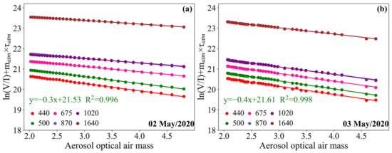
Figure 1.
The Lunar-Langley plots with ROLO model of Cimel#1662 performed in Lanzhou, China, on (a) 2 May and (b) 3 May 2020. The optimal least square linear fitting equation and correlation coefficient (R2) at 500 nm wavelength are displayed. The subscript ‘atm’ in Y-axis denotes the optical depth of Rayleigh scattering for air molecules.
3.3. Spectral Deconvolution Algorithm (SDA)
Ångström exponent (α) is defined as the slope of logarithm of versus logarithm of wavelength, which is usually utilized to represent the spectral wavelength dependence of and to supply a qualitative knowledge on aerosol particle size. In this study, we made use of a Log-linear fitting based on four wavelengths of 440, 500, 675 and 870 nm to calculate α according to the formula of . A spectral deconvolution algorithm (SDA) was used to extract the components of fine- and coarse-mode optical depths at 500 nm from the spectral total extinction AOD [44,45]. The SDA technique was mainly based on two basic hypotheses. The first was that the aerosol particle size distribution was effectively bimodal. The second assumption was that the coarse-mode Ångström exponent and its spectral variation were both approximately neutral. Specifically, the Ångström exponent and its second derivative () were the key inputs for running SDA procedure. These continuous function derivatives (generally computed at a reference wavelength of 500 nm) were acquired from a second-order polynomial fit of versus . The spectral AOD values used as input to SDA were limited to six wavelengths at 380, 440, 500, 675, 870 and 1020 nm.
3.4. Retrieval of Aerosol Vertical Profiles
The famous Mie scattering elastic lidar equation can be described as,
where z is the range-height between scattered particles and lidar, X(z) is the normalized range-corrected backscattering signal after dark-count, after-pulse noise, and incomplete geometric overlap factor corrections, C is a calibration constant of lidar, E is laser emitted pulse energy, β(z) and σ(z) are backscattering coefficient and extinction coefficient at z. The subscripts of a and m denote aerosol particle and air molecule, respectively.
The Mie scattering lidar equation is difficult to be directly solved, since there are two unknown variables (i.e., β(z) and σ(z)) in one equation. A lidar ratio is defined as the ratio of extinction coefficient to backscattering coefficient. Fernald [46] first designated a typical value of lidar ratio for a specific aerosol type and successfully attained an analytical solution of Mie lidar equation. Consequently, the vertical profiles of β(z) and σ(z) can be accurately calculated according to Equation (3). The lidar ratio of air molecule (Sm) has a constant value of 8π/3 which can be computed by the standard atmospheric profiles. The aerosol lidar ratio (Sa) is primarily reliant on aerosol species, chemical composition, and size distribution of particles, as well as on the wavelength of incident light [47]. As recommended by earlier researches [48,49,50], we designated Sa = 50 sr for dust aerosols, and Sa = 70 sr for urban polluted particles to retrieve the vertical profiles of backscattering and extinction coefficients in this study. The volumetric depolarization ratio (VDR) reflects the regular or irregular shapes of scattering particles. Overall, small VDR values (~0–0.1) correspond to fine-mode and spherical aerosols or cloud droplet particles, while large VDR values represent coarse-mode and nonspherical dust or ice crystal particles [51,52]. VDR was derived from the ratio of cross-polarized () and parallel () backscattering coefficients.
4. Results and Analysis
4.1. Two Heavy Dust Events Detected by Ground-Based Ozone Lidar
Figure 2 shows the spatial and temporal distributions of diverse meteorological element fields at Lanzhou obtained from hourly mean ERA5 reanalysis data from 5 to 12 April 2020. The distribution of air temperature (T) field presented an obvious stratified structure from the surface (~850 hPa) to 5.5 km height (~500 hPa) and a prominent diurnal variation within 3 km (~700 hPa). That is, the highest T (~292 K) appeared at the ground during daytime (i.e., 8 and 9 April) and the lowest T (~276 K) appeared at nighttime (i.e., 7 April), and T gradually decreased with the increase in altitude, which was mainly controlled by the incident net radiation flux. By contrast, the relative humidity field (RH) showed a more complex spatiotemporal variation and was dominated by dry and low RH (10~30% mostly after 8 April) airmass below 3 km. The wind vector fields at altitude of 500–700 hPa were dominated by the apparent prevailing westerlies in the mid-latitudes. The wind speed at 750–850 hPa height during clear-sky condition was relatively weak (2~4 m/s) and corresponding near-surface wind direction was complex and irregular. There were two intense cold front synoptic systems passing through Lanzhou on 6 to 7 April, and 9 to 10 April, respectively. The wind vector fields displayed a moderate intensity convergence ascending motion at low altitude (0~3 km) and a strong divergence sinking motion at high altitude from 3 to 5.5 km. The two cold front processes led to an intense sinking movement of upper air mass with maximum vertical wind speed of 1.0 Pa/s, which caused a sudden increase in vertical RH (70~95% on 6 and 7 April) and remarkable decrease in surface T (~284 K) during daytime. Accompanied by the cold front airmass, this was undoubtedly favorable to transport dust aerosols or air pollutants from surrounding areas to Lanzhou.
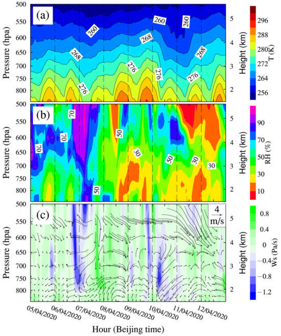
Figure 2.
Spatial and temporal distributions of diverse meteorological element fields obtained from hourly mean ERA5 reanalysis data. (a) Air temperature (T) in K, (b) relative humidity (RH) in %, and (c) horizontal wind vector in m/s (black arrows) and vertical wind speed in Pa/s (Ws, color bars) from 5 to 12 April 2020.
As mentioned above, Lanzhou is an important dust aerosol transport route and is often affected by dust storms every spring season. The ground-based DIAL lidar also successfully detected two strong dust events from 5 to 12 April 2020 appeared over Lanzhou. The first event occurred between 12:00 (local time) on April 6 and 20:00 on 7 April 2020, and the second dust intrusion appeared between 08:00 on 10 April and 13:00 on 11 April 2020, which corresponded well to the passing two cold fronts. Figure 3 illustrates the temporal evolution of vertical profiles of aerosol extinction coefficient, volumetric depolarization ratio, and ozone concentration derived from ozone lidar at Lanzhou during the period. We could see that aerosol extinction coefficients (σ) kept relatively low values (0.05~0.30 km−1) below 1 km height during 00:00–12:00 on 6 April, and there was an intense mixed layer of dust and clouds hanging over at 1.0–4.0 km from 12:00 on 6 April to 20:00 on 7 April, with σ values varying from 0.30 to 0.90 km−1, which was regarded as the transported dust particles from the remote desert regions. And the corresponding VDR changed from 0.03 to 0.10 below 1 km height before the first dust event, implying the dominated by fine-mode spherical particles, whereas the VDR values ranged from 0.15 to 0.55 at 1.0–4.0 km during the invasion of dust event, suggesting that the coarse-mode and non-spherical particles were predominant. Refs. [14,29] also indicated that the VDR was generally greater than 0.15 when dust events took place in Beijing and Lanzhou. There were some discrete and discontinuous signals of σ and VDR at 2.0–4.0 km, attributed to the influences of cloud layers, which were rejected after implementing quality control scheme. And the σ returned to background levels of 0.0~0.3 km−1 during the non-dusty days from 20:00 on 7 April to 06:00 on 10 April and the aerosol pollutants mainly accumulated below 500 m height, with the corresponding VDR of 0.03~0.12. However, there was an apparent layer of irregular aerosol particle continuously suspending at an altitude of 2.0–4.0 km with VDR of 0.15~0.22 during the non-dusty period where the vertical profiles of σ values stayed at a low level. Afterwards another intense dust layer occurred at 200 m to 4.0 km height from 08:00 on 10 April to 13:00 on 11 April 2020, with σ and VDR values of 0.4~1.5 km−1 and 0.15~0.30, respectively. The transregional dust aerosols were obviously transported from high altitude (~4.0 km) to the surface detected by DIAL lidar, which would seriously affect the air pollutions in both upper atmospheric layer and near the ground.
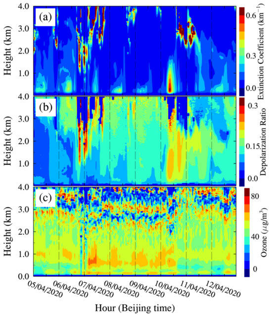
Figure 3.
Temporal evolution of vertical profiles of (a) aerosol extinction coefficient (km−1, top panel), (b) depolarization ratio (middle panel) and (c) ozone concentration in μg/m3 (bottom panel) derived from DIAL at Lanzhou from 5 to 12 April 2020.
Note that the intermittent interference signals at above 2 km height of ozone molecules were considered to be noise, which was possibly influenced by cloud layers or precipitation. Therefore, in this paper, we mainly investigated the ozone concentration distributions at 0.10–2.0 km. Figure 3c shows that the vertical structures of ozone concentrations were distinct and continuous with high values (52~80 μg/m3) located at 0.10–1.5 km. The diurnal variations of ozone concentrations exhibited a remarkable pattern that the maximum ozone value at 0.50–1.30 km was found during nighttime (i.e., from 6 April to 10), while the highest ozone concentration at 0.20 km usually appeared during the afternoon of daytime. In other words, the low-level ozone concentrations gradually increased with the intensity of incoming solar radiation in the morning, and reached a maximum peak of ~80 μg/m3 at 14:00–16:00, and then gradually decreased with the weakening of solar radiation before sunset. Affected by cold front processes, the gaseous precursors (e.g., NO2 and VOCs) and incoming solar radiation near the ground were significantly reduced. Therefore, the diurnal changes of ozone concentration were very weak and even disappeared at 0.50–1.3 km after the two dust events, as presented in Figure 3c. Nevertheless, near-surface ozone concentration still showed an evident diurnal variation after dust process.
4.2. Aerosol Vertical Profiles and Optical Properties Affected by Dust Events
Figure 4 delineates the hourly average vertical profiles of σ and VDR at different hours during the incursion of second heavy dust event. There were two evident dust layers appearing at 300 m and 2.5–3.0 km heights on 10 April, which were highly consistent with the aforementioned aerosol vertical structures. At 08:00 on 10 April, the σ apparently increased from 0.15 km−1 at 100 m to 0.62 km−1 at 300 m, and linearly decreased with the altitude, up to a minimum value of 0.01 km−1 at 2 km. And the corresponding VDR remained at a stable value of 0.20~0.23 from 300 m to 1.50 km and decreased up to 0.12 at about 2.0 km. At 14:00 on 10 April, the σ varied from 0.10 km−1 to 0.19 km−1 within 200 m to 2.0 km, and corresponding VDR kept at 0.15 to 0.18. During the intrusion of dust plume, several obvious dust layers were majorly located at altitudes between 2 and 4 km with maximum σ and VDR of 1.30 km−1 and 0.35. For instance, the σ below 2.3 km at 20:00 on 10 April kept a steady low value of 0.08 km−1 and markedly increased with height, and up to a maximum of 1.16 km−1 at 2.80 km. The corresponding VDR at 0.10–2.3 km ranged from 0.15 to 0.20 and reached a maximum of 0.30. The error bars of σ and VDR clearly increased with the altitude and attained a maximum value at the intense dust layer. Note that the VDR obviously decreased with the height from 2.3 km to 2.8 km, attributing to the influences of cloud contamination that had been eliminated after data quality control. At 14:00 on 11 April, the intensity of dust event significantly reduced, and the σ and VDR remained at 0.10~0.16 km−1 and 0.10~0.18, respectively from 100 m to 3.0 km height. This indicated that the dust event gradually abated and vanished. The intensities of two dust events were comparable to that of the dust storm occurred in Lanzhou from 9 to 12 March 2013 [29].
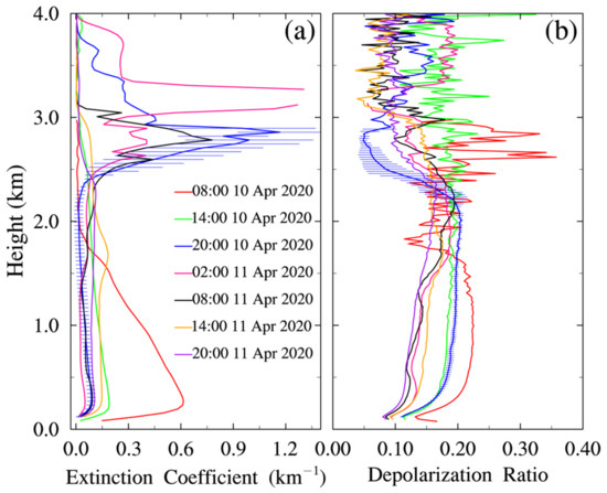
Figure 4.
Vertical profiles of (a) aerosol extinction coefficient (km−1) and (b) depolarization ratio at different hours during the invasion of a heavy dust event from 10 to 11 April 2020. Two distinct dust layers appear at 300 m and 2.5–3.0 km heights on 10 April 2020, respectively. The error bars represent the hourly average values plus or minus one standard deviation.
Figure 5 draws daytime and nighttime variations of spectral AOD, Ångström exponent (AE440–870nm), SDA coarse-mode and fine-mode AOD500, and fine-mode fraction (FMF) at Lanzhou from 5 to 12 April 2020. The gray backdrop represents the nighttime measurement from CE318-T photometer. The FMF is defined as fine-mode AOD500 divided by total AOD500, which reflects the proportion of fine-mode particles in the columnar atmosphere. It is obvious that columnar AOD500 maintained a steady low value of 0.20~0.40 under non-dusty days and corresponding AE440–870nm and FMF varied from 0.60 to 1.50, and from 0.50 to 0.82, which suggested that fine-mode particles were dominant under clear-sky conditions. In contrast, AOD500 values were larger than 0.50 (0.50~3.0) and AE440–870nm were less than 0.50 (0.10~0.50) under dusty cases, and corresponding FMF values rangeed from 0.20 to 0.50, which implied that coarse particles were mainly predominated [26,27]. This indicated that the atmospheric columnar AOD values in Lanzhou increased by three to eight times under the influences of trans-regional transport of high-altitude dust events. The missing measurements of AOD due to cloud contamination impacts corresponded well to the two intense dust invasion periods, which directly demonstrated that the cloud screening algorithm used in this study was robust and also further corroborated that the cloud and dust layers detected by DIAL Lidar during two dust events in Figure 3 were reliable.
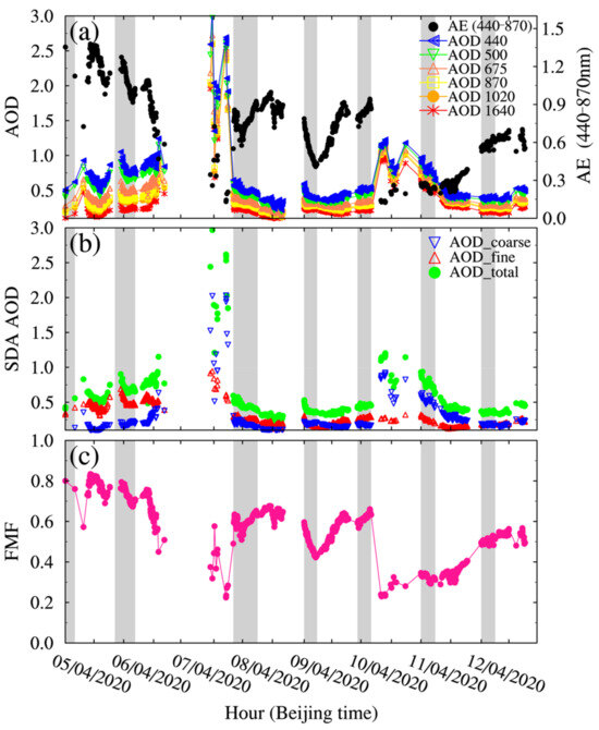
Figure 5.
Time series of (a) spectral aerosol optical depth (AOD) at diverse wavelengths vs. Ångström exponent (440–870 nm), (b) spectral deconvolution algorithm (SDA) calculated coarse-mode (blue), fine-mode (red) and total (green) AOD at 500 nm, and (c) SDA fine-mode fraction (FMF) at Lanzhou from 5 to 12 April 2020. The gray backdrop indicates the nighttime observations from CE318-T sun-sky-lunar photometer.
Figure 6 describes the time evolutions of hourly mean mass concentrations of six air pollutants and the ratio of PM2.5/PM10 at Lanzhou derived from China National Environmental Monitoring Center (CNEMC). Before the invasion of dust events, the surface particle mass concentrations in Lanzhou remained at a stable background level from 5 to 9 April 2020, with PM2.5, PM10 concentrations and PM2.5/PM10 of 50 μg/m3, 100 μg/m3, and 0.40~0.75, respectively. It seemed that the concentrations of surface particulate matters were not significantly influenced by the intrusion of first dust event. Affected by the contribution of second strong dust event transportation, the surface PM10 concentrations sharply rose and strikingly increased from 100 μg/m3 at 06:00 to 200~590 μg/m3 at 07:00–10:00 on 10 April, which were about 3~11 times greater than World Health Organization Air Quality Guidelines of 50 μg/m3 for PM10 (24 h average) [53]. And the increases of PM2.5 concentrations were relatively smaller, ranging from 50 to 134 μg/m3, and corresponding ratios of PM2.5/PM10 were less than 0.15. This again confirmed that the coarse-mode particles significantly were dominated at near-surface during the invasion of second dust event. After the dust process, the PM10 concentrations rapidly decreased (~150 μg/m3) but were slightly higher than the background level (~100 μg/m3), with PM2.5/PM10 ratio of 0.20~0.50, revealing that coarse-mode particles were still predominated. The concentrations of other air pollutants exhibited a noticeable single-peak diurnalvariation. The SO2 and CO concentrations usually appeared a maximum value at every 08:00–10:00 and O3 generally reached a peak value at 14:00–16:00. The maximum NO2 concentration occurred at 22:00–00:00 under dust cases, but commonly occurred at 08:00–12:00 under non-dusty conditions. This was primarily dependent on emissions from various human activities, complex photochemical reactions of air pollutant and diluted diffusion conditions (e.g., vertical convection exchange). The concentrations of SO2, NO2, CO, and O3 ranged from 0~72 μg/m3, 0~150 μg/m3, 0~6.0 mg/m3, and 0~135 μg/m3, respectively. It was distinct that concentrations of air pollutants displayed a pronounced decrease after the second dust event, mainly attributable to powerful dilutive diffusion ability caused by the cold front. However, the corresponding O3 concentrations firstly presented a slight decrease (70~85 μg/m3), and quickly returned to high values of 110~135 μg/m3, owing to the complexity of formation process of ozone. These results were well coincident with the vertical profile of ozone concentration detected by DIAL lidar. The surface O3 concentrations usually attained a minimum value (8~10 μg/m3) appeared at nighttime period, which was due to the synergistic effect of calm weather and NO titration [35].
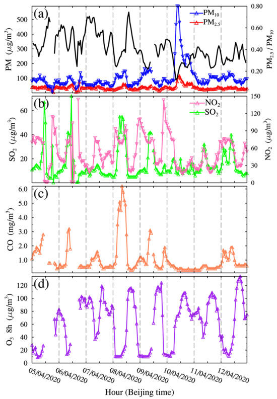
Figure 6.
Time evolutions of hourly mean mass concentrations of six different air pollutants at Lanzhou derived from China National Environmental Monitoring Center (CNEMC). (a) PM10 and PM2.5 in μg/m3 vs. the ratio of PM2.5/PM10 (black curve), (b) SO2 vs. NO2 in μg/m3, (c) CO in mg/m3, and (d) 8 h mean of O3 in μg/m3 from 5 April to 12 April 2020.
4.3. A Serious Haze Episode Identified by Ground-based Ozone Lidar
Figure 7 is the same as Figure 2, except that the dates are from 30 December 2020 to 2 January 2021. The stratified structure of air temperature field from the surface (~850 hPa) to 5.5 km (~500 hPa) height still existed during the winter cases, but the diurnal variation of T from 0 to 2.5 km was relatively weak, with the highest T (~275 K) occurring at 15:00 on 1 January 2021, which was clearly lower than that on 8 April 2020 (~292 K). This was majorly due to the significantly weaker solar radiation intensity and shorter sunshine duration reaching the surface during winter period. The RH field showed that the upper layer (3~5.5 km) was overwhelmingly dominated by very dry and cold air masses (RH of 10~30%) during the whole period, while the lower layer (0~3.0 km) was dominated by weakly warm and humid air masses (RH of 30~70%). The RH value at nighttime (50~70%) was slightly higher than that in daytime (30~40%), which was opposite to diurnal variation of T and could be explained by the classical Clausius-Clapeyron equation. The wind vector field in upper layer (500~700 hPa) presented strong and stable westerlies with wind speeds greater than 12 m/s, while the lower layer (0~3.0 km) displayed irregular wind direction and very weak wind speed (<1.0 m/s). This intense calm and stable atmosphere inversion layer were very conducive to the widespread accumulation of low-level air pollutants and deteriorated the local ambient air quality. The calm and stable weather processes lasted until 12:00 on 2 January 2021, and a strong northeasterly wind (3~6 m/s) and a moderate vertical ascending convective movement (−0.6 Pa/s) began to appear in Lanzhou since 13:00, which would greatly strengthen the dilution and diffusion capacity of surface air pollutants. An interesting phenomenon was that the upper layer air masses exhibited a distinct subsiding motion during 00:00–12:00 on 30 December 2020 and there was a strong cold and moist Tongue extending from 3.0 km to the surface, with T of 255~260 K and RH of 60~90%.
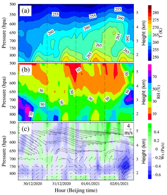
Figure 7.
The same as Figure 2, except that the dates are from 30 December 2020 to 2 January 2021.
The DIAL lidar perfectly captured a heavy haze pollution process from 31 December 2020 to 2 February 2021, as showed in Figure 8. From 00:00 to 03:00 on 30 December 2020, an obvious layer with high σ appeared at an altitude of 1.0–2.0 km over Lanzhou and the corresponding σ and VDR values varied from 0.30 km−1 to 0.65 km−1, and from 0.06 to 0.15, respectively. This was most likely caused by the aloft aerosols particles subsiding into the lower-layer atmosphere carried by the cold and moist Tongue system, as confirmed in Section 4.3. A gradual increasing pollution level of a heavy haze episode from 31 December 2020 to 2 January 2021 occurred over Lanzhou was completely detected by ground-based DIAL lidar. From Figure 8a, we knew that the air pollutants and aerosol particles primarily accumulated within 0.10–1.0 km height, and the largest σ value was located at 0.20–0.80 km. And the maximum σ changed from 0.50 km−1 on 31 December 2020 to 0.60 km−1 on 1 January and 0.68 km−1 on 2 January 2021, whereas the VDR value remained stably at 0.03~0.12 throughout the haze pollution process. This directly demonstrated that the fine-mode and spherical aerosol particles were predominant during the heavy haze period [14,16]. Diverse gaseous precursors emitted by human activities were firmly trapped in PBL under calm and stable thermal inversion layer and hard to spread out, which readily generated different types of aerosol particles through various complex liquid phase chemical reactions or photochemical reactions. Therefore, the heavy haze episode was gradually intensified and lasted for several days under high moist and strong sunlight conditions. Note that the worsening haze pollution process began to weaken since 16:00 on 2 January, attributable to a strong northeasterly wind (3~6 m/s) and a moderate vertical ascending convective movement (−0.6 Pa/s) appearing in Lanzhou since 13:00, as indicated in Section 4.3.
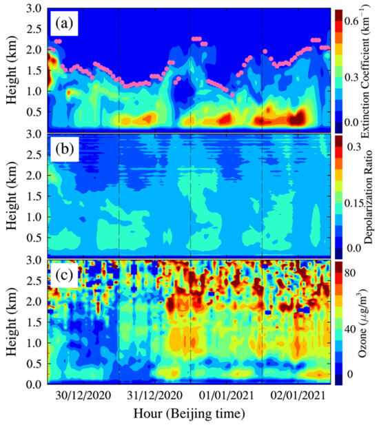
Figure 8.
The same as Figure 3, except that the dates are from 30 December 2020 to 2 January 2021. And the aerosol mixing layer heights (pink solid circle) determined from DIAL are superimposed in (a).
In contrast, the profile of ozone concentration exhibited a distinct two-layer structure, with the first layer at 0.60–1.40 km height and the second layer at 0.10–0.30 km. A discernible characteristic was that the highest O3 concentration of the first ozone layer generally appeared between 20:00–02:00 at nighttime, with a maximum of 72 μg/m3, while the second layer commonly occurred between 14:00–16:00 at daytime, with a maximum of 60 μg/m3. This suggested that the formation mechanism and process of ozone at diverse altitudes were different in Lanzhou, which was worth investigating in the future study. And there was also a distinct ozone layer of high O3 concentration at the altitude of 0.10–1.0 km from 00:00 to 03:00 on 30 December 2020.
As mentioned-above, the concentrations of aerosol particles or air pollutants are very high in the atmospheric boundary layer (ABL), whereas they sharply decrease in free atmosphere. Thereby, the aerosol mixing layer height (AMLH) is defined as the height at which aerosol particles gradient is apparently discontinuous. Note that the AMLH majorly represents the vertical distribution of aerosol in lower atmosphere, and is slightly different from the traditional ABL height. The range-corrected backscattering signal profile X(z) = P(z)z2 can represent the vertical distribution of aerosol concentrations, hence AMLH is calculated by the gradient method. In this study, the AMLH was designated as the height at which X(z) evidently decreased with z, and corresponding height at the minimum of [34,54]. From Figure 8a, the AMLH showed a prominent pattern of diurnal variation, with the highest value of 1.5~2.0 km occurring during daytime and the lowest value of 0.80~1.0 km occurring at nighttime or during haze periods. The AMLH at Lanzhou from 5 to 12 April 2020 could not reasonably be retrieved according to the gradient method, mainly because of the drastic fluctuations of backscattering signals caused by elevated dust aerosol and cloud layer.
4.4. Aerosol Vertical Profiles and Optical Properties Affected by Haze Episode
Figure 9 once again completely outlines the gradual intensification process of severe haze pollution episode in Lanzhou from 22:00 on 1 to 12:00 on 2 January 2021. The large σ values (0.50~0.68 km−1) were primarily concentrated at a height of 0.10–0.70 km, and the highest σ of ~0.68 km−1 appeared at 0.30 km on 13:00 of 2 January. Afterwards, the heavy haze process began to weaken since 14:00 on 2 January and the maximum σ was 0.35 km−1, which was consonant with the results of Figure 8. In comparison, the VDR values at 0.10–2.0 km always remained stable in the range of 0.08~0.11 throughout the haze episode, which indicated that the spherical and fine aerosol particles were dominant in Lanzhou during the winter domestic heating period.
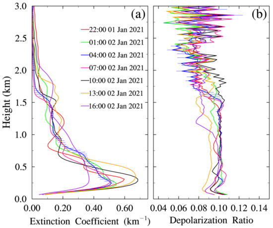
Figure 9.
The same as Figure 4, except that the dates are from 1 to 2 January 2021. There is an apparent layer of air pollutant at 100–700 m height, and the air pollutant concentrations significantly increase from 22:00 on 1 January to 13:00 on 2 January 2021.
Figure 10 characterizes time series of spectral AOD, AE440–870nm, SDA coarse- and fine-mode AOD500, and FMF at Lanzhou from 30 December 2020 to 2 January 2021. It is clear that the columnar AOD, AE440–870nm, and fine-mode AOD500 values increased significantly with the gradual aggravation of heavy haze process, and the AOD500 increased from 0.25~0.36 on 30 December to 0.40~0.45 on 31 December 2020 to 0.35~0.50 on 1 January, and eventually attained the largest value of 0.55~0.65 on 2 January 2021. And the corresponding AE440–870nm remained consistently elevated values (0.80~1.50) with the increase in AOD during the whole haze period. Note that the fine-mode AOD500 of haze particles showed a prominent diurnal variation, while the coarse-mode AOD500 was usually low and nearly constant. The FMF values steadily increased from 0.60 on 30 December to 0.85 on 2 January. This confirmed that fine pollution particles were the major contributors to AOD in Lanzhou during the severe haze event in January 2021. There were only a few cases of coarse-mode AOD500 to be comparable with the fine-mode AOD500 (e.g., 30 and 31 December, with FMF of 0.35~0.50), probably attributed to the dust intrusion or the residual cloud contamination. Ref. [16] uncovered that the maximum of σ, VDR, AOD500, AE440–870nm and FMF in Xuzhou were 1.0 km−1, 0.10 ± 0.01, 0.68 ± 0.26, 1.30 ± 0.12 and 0.81 ± 0.09, respectively, during heavy haze event, which were comparable to the results of this study.
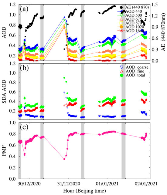
Figure 10.
The same as Figure 5, except that the dates are from 30 December 2020 to 2 January 2021. This is a typical haze pollution process during the winter domestic heating period.
From Figure 11, we could see that the mass concentrations of surface six air pollutants and ratio of PM2.5/PM10 increased strikingly from 30 December 2020 to 2 January 2021, and reached a highest value at 13:00 on 2 January, then suddenly decrease since 14:00 on 2 January, which was coincident with the aerosol vertical profiles and variations of spectral AOD behaviors. For example, the PM2.5 and PM10 concentrations and ratio of PM2.5/PM10 steadily increased from 15 μg/m3, 30 μg/m3, and 0.45 on 30 December to 110 μg/m3, 180 μg/m3, and 0.68 on 2 January, respectively, and then sharply reduced up to 20 μg/m3, 40 μg/m3, 0.58 at 00:00 on 3 January. The time series of PM concentrations exhibited a consistent variation with the total and fine-mode AOD500. The SO2, NO2, and CO concentrations ranged from 8~60 μg/m3, 20~112 μg/m3, and 0.5~4.5 mg/m3 during the entire period, and dramatically decreased up to 15 μg/m3, 46 μg/m3, and 1.0 mg/m3 at 00:00 on 3rd January, respectively, which were smaller than the corresponding maximums of 163.5 ± 7.4 μg/m3, 159.2 ± 9.3 μg/m3, and 5.4 ± 0.06 mg/m3 in Lanzhou during domestic heating seasons from 2013–2016 [20]. These findings well corroborated that air pollutants or aerosol particles produced in the heavy haze event presented a consistent variation characteristic at both ground level and upper atmospheric layer observed by different techniques. In contrast, the diurnal variation of surface ozone concentration was different from that of other gaseous pollutants and upper-level vertical profiles of ozone concentration. That was, the surface O3 concentration reached a maximum of 80 μg/m3 appeared at 12:00 on 30 December, and rapidly declined with time and attained a minimum value of 5 μg/m3 on 2 January. Although the ozone concentration also displayed a largest value in the afternoon during daytime and a lowest value at nighttime, the peak value of O3 was only 30 μg/m3 during the heavy haze episode, which was much smaller than that before haze event (~80 μg/m3) and the value at lower atmospheric layer of 0.10–1.4 km (60~72 μg/m3). This was because the large accumulation of high concentration haze particles in upper air effectively impeded and reduced solar radiation arriving at the Earth’s surface, weakened the photochemical reaction rate, and ultimately were not conducive to the production of ground-level ozone gas.
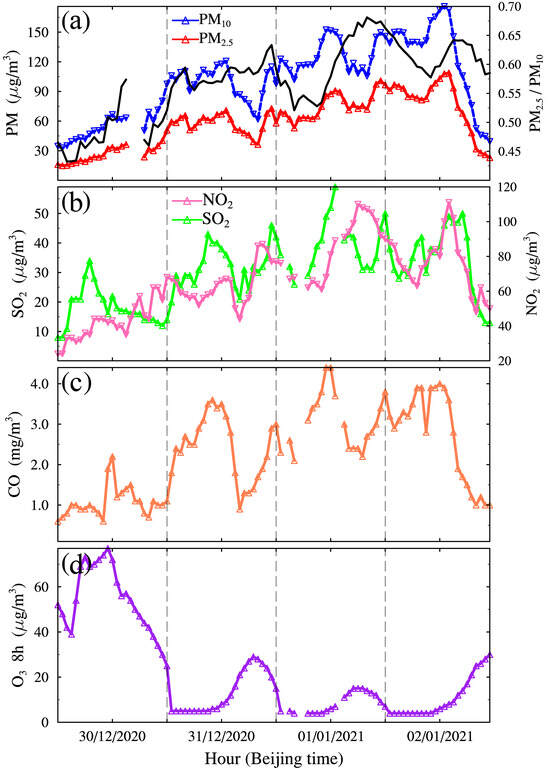
Figure 11.
The same as Figure 6, except that the dates are from 30 December 2020 to 2 January 2021.
4.5. Retrieval of Surface Particulate Mass Concentration
As mentioned-above, the aerosol extinction coefficient profile is a good indicator for characterizing aerosol particle concentration. When the aerosol particles in ABL are uniformly mixed, the σ at a certain height would have a good linear relationship with the surface particulate mass concentrations (i.e., PM2.5, PM10). Table 2 summarizes the linear fitting formulae and correlation coefficients (R) between ground-based measured dry PM2.5 and PM10 concentrations and 532 nm σ at different levels of height (0.09~0.21 km) from 5 to 12 April 2020. Note that σ profiles in the real atmosphere were observed by DIAL lidar. In order to improve the reasonability of fitting equation, we removed the data points with RH exceeding 80% in this study. It was clear that σ at 0.09 km height exhibited the best linear fitting result. For instance, the fitting formula and R of dry PM2.5 were y = 286.41x + 28.96 and 0.71, respectively. The fitting results showed a gradual decrease with the increase in height, which was mainly caused by the intrusion of dust events and transported of aloft dust particles into the ground in different degrees. Table 3 is the same as Table 2, except that the dates are from 30 December 2020 to 2 January 2021. In general, the linear fitting formulae between σ at different heights and surface PM2.5 or PM10 concentrations presented a better relationship under heavy haze episodes than those in dust cases, which implied that the degree of uniform mixing of aerosol particles from near the ground to 210 m in haze pollution conditions was better than that in dust events. Interestingly, the fitting results showed an apparent increase with the increase in height and the fitting formula and R between σ at 0.21 km and surface PM10 concentration were y = 164.01x − 0.46, and 0.934, respectively. Therefore, we made use of the σ at 0.09 km (or 0.21 km) with RH < 80% to implement the best linear fitting with surface dry PM2.5 and PM10 concentrations under dust events (or heavy haze episodes) in this study.
Table 2.
The linear fitting results between surface PM2.5, PM10 concentrations and 532 nm aerosol extinction coefficients at different heights (0.09~0.21 km) from 5 to12 April 2020.
Table 3.
The same as Table 2, except that the dates are from 30 December 2020 to 2 January 2021.
Figure 12 depicts the time series of hourly average σ at 0.09 km (RH < 80%) observed by DIAL lidar versus surface PM2.5 or PM10 concentrations at Lanzhou from 5 to 12 April 2020. The scatterplots of linear fitting PM2.5 and PM10 concentrations from σ at 0.09 km and PM2.5 and PM10 concentrations are also given in Figure 12. Generally, hourly average σ at 0.09 km displayed a good diurnal variation with surface PM2.5 and PM10 concentrations, especially under severe dust events. And the consistency between mean σ and PM10 concentration seemed to be better than that for PM2.5 concentration, which was expected. Overall, the linear fitting PM2.5 and PM10 concentrations were consistent with the in situ PM concentrations, and the fitting values were somewhat smaller than those in situ measurements. For example, the root mean square error (RMSE) between estimated and measured PM10 concentration was 51.27 μg/m3, with relative bias (RE) of 31.21%. And the RMSE between estimated and measured PM2.5 concentration was 12.47 μg/m3, with the RE of 20.16%.
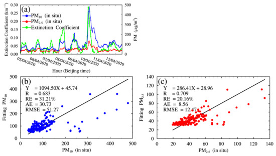
Figure 12.
(a) Time series of hourly average aerosol extinction coefficient at 90 m height observed by DIAL Lidar vs. mass concentrations of PM10 and PM2.5 at Lanzhou from 5 to 12 April, 2020. (b) Fitting PM10 concentrations by extinction coefficient at 0.09 km height and PM10 in situ. (c) Fitting PM2.5 concentrations by extinction coefficient at 0.09 km height and PM2.5 in situ. The linear fitting equations of PM mass concentration and extinction coefficient are shown in the figure.
As well know that, AOD is the total integral of columnar aerosol extinction coefficient in actual atmosphere, while PM2.5 represents the mass concentration of surface dry aerosol particle. The PM2.5 mass concentration is estimated based on measured AOD values and has to be successively carried out humidity correction and vertical height correction. A simplified PM2.5 remote sensing method (PMRS) was generally used to estimate the surface dry PM2.5 concentration by synergistic observations of daytime and nighttime AOD, RH, AMLH, constraint of AOD particle size, relative humidity and vertical height correction, volume conversion and mass transformation [55,56]. The PMRS model is majorly based on three basic assumptions: (i) All of aerosol particulate matters are uniformly mixed in a homogeneous layer within the PBLH; (ii) Aerosol light-absorption properties and size distributions are independent with height; (iii) The hygroscopic properties of aerosols are independent of particle size. The estimated PM2.5 mass concentration (PM2.5,estimated) can be expressed as,
where AOD and FMF are measured by CE318-T photometer, VEf is volumetric visualization factor that is a quadratic polynomial function of FMF, PBLH is planetary atmospheric boundary layer height, which is equivalent to AMLH in this study, f(RH) is the humidity correction factor, and is density of dry PM2.5 particulate, which is designated as a typical value of 1.50 g/cm3 in northern China [57]. According to Li et al. [56], the VEf and f(RH) are given by,
where RH is obtained from ERA5 products. For a typical continental aerosol, the coefficients of a and b are 0.99 and 0.16, respectively. Therefore, we can reasonably estimate PM2.5 mass concentration based on the daytime and nocturnal AOD values.
Figure 13 delineates the time series of hourly average σ at 0.21 km observed by DIAL lidar versus surface PM2.5 and PM10 concentrations as well as PM2.5,estimated (PMRS) at Lanzhou from 30 December 2020 to 2 January 2021. The scatterplots of between PM2.5,estimated (PMRS), fitting PM2.5 or PM10 and in situ PM concentrations were showed in Figure 13b,c. It was distinct that the hourly mean σ at 0.21 km displayed a consistent variation with surface PM10 or PM2.5 concentrations during the entire period. Note that the linear fitting PM concentrations from σ at 0.21 km were obviously better than that in PMRS method. Namely, the PM2.5,estimated (PMRS) at Lanzhou were much lower than the surface measured PM2.5 concentration, suggesting that larger uncertainty of PMRS model might be originated from the retrieval errors of FMF, VEf, , AMLH, and f(RH), which should be greatly improved in the future. The RMSE between estimated and measured PM10 concentration was 13.35 μg/m3, with the RE of 13.38%. And the RMSE between estimated and measured PM2.5 concentration was 10.96 μg/m3, with RE of 19.81%. These results demonstrated that the aerosol extinction coefficient profile observed from lidar was a good surrogate to estimate surface PM2.5 and PM10 mass concentrations, which was deserved to further study at diverse sites and under different polluted conditions in the future.
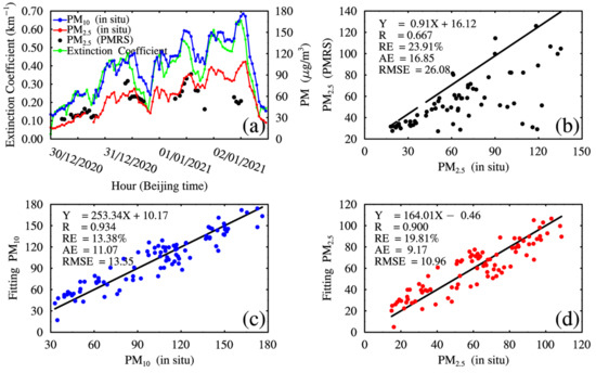
Figure 13.
(a) Time series of hourly average aerosol extinction coefficient at 210 m height observed by DIAL vs. mass concentrations of PM10 and PM2.5, and PM2.5 concentration calculated by PMRS method at Lanzhou from 30 December 2020 to 2 January 2021. (b) Scatterplot of the PM2.5 mass concentration measured by ground-based observations and calculated by PMRS method. (c) Fitting PM10 concentrations by extinction coefficient at 0.21 km height and PM10 in situ. (d) Fitting PM2.5 concentrations by extinction coefficient at 0.21 km height and PM2.5 in situ. The linear fitting equation is displayed with thick black line.
4.6. Source and Aerosol Types during Dust Haze Events
Figure 14 shows the NOAA HYSPLIT Model simulated 72 h backward trajectories at 500 m (red), 1500 m (blue) and 3000 m (green) above ground level reaching Lanzhou at (a) UTC 00 on 10 April 2020 and (b) UTC 06 on 2 January 2021. The altitude of each back-trajectory as a function of time is also reported. It is clear that three major air masses at different altitudes originated from remote Taklimakan desert or Gobi deserts and reached at Lanzhou on 10 April 2020, which contributed abundant dust particles to the upper layer and the ground of Lanzhou. This result was firmly corroborated by the synergistic observations of DIAL lidar, CE318-T photometer, and surface particulate concentrations at Lanzhou. The low-level (500 m AGL) airmass mainly stemed from the Great Gobi desert in southwest of Mongolia, and traveled northwest and passed through northern Inner Mongolia. At UTC 00:00 on 9 April, the airmass suddenly turned to northeast, and arrived at Lanzhou. The middle-level (1500 m AGL) airmass descended from the Gobi deserts of Hexi Corridor in northwest China and reached at Lanzhou. And the upper-level (3000 m AGL) airmass originated from Taklimakan Desert, and transfered to northwest, eventually arrived at the upper atmosphere above Lanzhou. In contrast, the low-altitude (500 m AGL) airmass on 2 January 2021 primarily arose from the surrounding area of Lanzhou, which produced a great amount of air pollutants during the domestic heating season. This would directly exacerbate the intensity of haze polluted episode in Lanzhou and the heavy haze events lasted for a long period under calm and stable atmospheric conditions. Both the middle-level (1500 m AGL) and upper-level (3000 m AGL) airmasses resulted from Afghanistan, Pakistan, and western China, and traveled westward through Qaidam Basin and arrived at Lanzhou. Compared with the dust cases in April 2020, the main airmass of heavy haze episode in January 2021 at Lanzhou mostly came from the lower atmosphere around the neighboring regions.
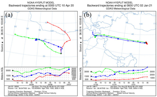
Figure 14.
The NOAA HYSPLIT Model simulated the 72 h backward trajectories at 500 m (red), 1500 m (blue) and 3000 m (green) above ground level reaching Lanzhou at (a) UTC 00 on 10 April 2020 and (b) UTC 06 on 2 January 2021. The altitude of each back-trajectory as a function of time is also reported. The five-pointed star represents Lanzhou site.
5. Summary
Based on synergistic observations of ground-based DIAL ozone lidar, CE318-T sun-sky-lunar photometer, particulate matter mass concentrations and reanalysis datasets, this study comprehensively investigated aerosol vertical structure and optical properties during two heavy dust and haze events in a typical valley basin city, Lanzhou of northwest China. The main conclusions are summarized as followings.
Dust particles originated from Taklimakan Desert in Xinjiang and the Great Gobi desert in southwest Mongolia traveled eastward or northeastward at different altitudes under intense cold front synoptic systems, and reached Lanzhou at 08:00 on 10 April 2020, which was demonstrated by the HYSPLIT 4.0 backward trajectory model. The DIAL lidar also successfully detected the entire strong dust event from 5 to 12 April 2020 appeared over Lanzhou. The trans-regional aloft dust particles were entrained into the ground from high altitude (~4.0 km), and led to significant changes of vertical profiles of aerosol optical properties in Lanzhou. The maximum σ, VDR, AOD500, surface PM10 and PM2.5 concentrations attained 0.4~1.5 km−1, 0.15~0.30, 0.5~3.0, 200~590 μg/m3 and 134 μg/m3, respectively under heavy dust event, which were 3 to 11 times greater than those at background level. While the corresponding AE440–870, FMF and PM2.5/PM10 values steadily remained at 0.10~0.50, 0.20~0.50, and 0.20~0.50, respectively, suggesting that coarse-mode and irregular non-spherical particles were overwhelmingly dominant. The surface air pollutants (SO2, NO2, and CO) at Lanzhou exhibited a pronounced decrease after the dust event, whereas the corresponding O3 concentrations firstly showed a slight decrease (70~85 μg/m3), and quickly returned to high values of 110~135 μg/m3, owing to the complexity of formation process of ozone. In contrast, the maximum O3 concentrations at 0.50–1.30 km appeared in nighttime (from 6 to 10 April) and became very weak after the dust event, while the maximum O3 concentrations at 0.20 km occurred in the afternoon and still showed an evident diurnal variation after dust plume.
A heavy haze episode stemmed from local emissions appeared at Lanzhou from 30 December 2020 to 2 January 2021. The low-altitude transboundary transport aerosols seriously deteriorated the air quality level in Lanzhou, and the aerosol loading, surface air pollutants and fine-mode particles markedly increased during the gradual strengthening of haze process. The maximum σ at 0.20–0.80 km, AOD500, AE440–870nm, FMF, PM2.5 and PM10 concentrations, and PM2.5/PM10 remarkably increased from 0.50 km−1, 0.25, 0.80, 0.60, 15 μg/m3, 30 μg/m3, 0.45 at 30 December 2020 to 0.68 km−1, 0.65, 1.50, 0.85, 110 μg/m3, 180 μg/m3, 0.68 at 2 January, while the corresponding VDR steadily kept at 0.03~0.12, implying that the fine-mode and spherical small particles were predominant during the haze episode. The profile of ozone concentration exhibited a prominent two-layer structure, with the first layer at 0.60–1.40 km height appearing between 20:00–02:00 during nighttime and the second layer at 0.10–0.30 km occurring between 14:00–16:00 during daytime. Both ozone concentrations at two heights always kept high levels (i.e., 72 and 60 μg/m3) during the entire period. Conversely, surface ozone concentration showed a significant decrease during severe haze period, with the peak value of 20~30 μg/m3, which was much smaller than that before haze pollution (~80 μg/m3 on 30 December). This indicated that the sources of ozone formation at diverse altitudes during haze episode in Lanzhou were different and very complex, which deserved to be further explored.
The aerosol extinction coefficients at different heights (0.09~0.21 km) showed a good positive correlation with surface PM10 or PM2.5 mass concentrations in Lanzhou during dust or haze events when aerosol particles were uniformly mixed within PBLH. The linear fitting relationship between hourly average σ at 0.21 km and surface PM2.5 or PM10 concentration during severe haze episode presented much better than that in PMRS method, attributable to larger uncertainty of PMRS model’s inputs. This result implied that the vertical profile of aerosol extinction coefficient was a good surrogate for evaluating the mass concentrations of surface particulate matters under uniformly mixed aerosol layers conditions, which was of great scientific significance for retrieving surface air pollutants in remote desert or ocean regions. These statistics of the aerosol vertical profiles and optical properties under heavy dust and haze events in Lanzhou were helpful to investigate and validate the trans-regional transportation and radiative forcing of aloft aerosols in the application of climate models or satellite remote sensing.
Author Contributions
Conceptualization, J.M. and J.B.; methodology, J.M. and J.B.; software, J.M., J.B., B.L. and D.Z.; investigation, J.M. and J.B.; Writing—Original draft preparation, J.M. and J.B.; Writing—Review and editing, B.L., D.Z. and X.W.; visualization, J.M. and J.B.; data observation and instruments maintenance, Z.M. and J.S.; supervision, J.B.; project administration, J.B.; funding acquisition, J.B. All authors have read and agreed to the published version of the manuscript.
Funding
This work is jointly supported by the National Natural Science Foundation of China (42075126), Gansu Provincial Science and Technology Innovative Talent Program: High-level Talent and Innovative Team Special Project (Chief Scientist System, No. 22JR9KA001), Project of Field Scientific Observation and Research Station of Gansu Province (18JR2RA013), and the Fundamental Research Funds for the Central Universities (lzujbky-2022-kb11).
Data Availability Statement
The surface hourly averaged six air pollutants (PM2.5, PM10, SO2, NO2, CO and O3) at Lanzhou station were provided by CNEMC (http://www.cnemc.cn/, accessed on 8 March 2023). ERA5 reanalysis datasets were acquired from the ECMWF (https://cds.climate.copernicus.eu/cdsapp#!/search?type=dataset, accessed on 16 March 2023). The HYSPLIT 4.0 model was downloaded from Air Resources Laboratory of NOAA (https://www.ready.noaa.gov/HYSPLIT.php, accessed on 18 March 2023). The original contributions presented in the study are included in the article, further inquiries can be directed to the corresponding author.
Acknowledgments
The authors thank the CNEMC, ECMWF, NOAA’s HYSPLIT and NASA-USGS teams for supplying the ground-based observations, reanalysis products, and ROLO model used in this study. We also appreciate the editors and all reviewers for their insightful and valuable comments.
Conflicts of Interest
The authors declare no conflicts of interest.
References
- Huang, J.; Wang, T.; Wang, W.; Li, Z.; Yan, H. Climate effects of dust aerosols over East Asian arid and semiarid regions. J. Geophys. Res. 2014, 119, 11398–11416. [Google Scholar] [CrossRef]
- Bi, J.; Huang, J.; Holben, B.; Zhang, G. Comparison of key absorption and optical properties between pure and transported anthropogenic dust over East and Central Asia. Atmos. Chem. Phys. 2016, 16, 15501–15516. [Google Scholar] [CrossRef]
- Li, Z.; Lau, W.K.-M.; Ramanathan, V.; Wu, G.; Ding, Y.; Manoj, M.G.; Liu, J.; Qian, Y.; Li, J.; Zhou, T.; et al. Aerosol and monsoon climate interactions over Asia. Rev. Geophys. 2016, 54, 866–929. [Google Scholar] [CrossRef]
- Twomey, S. The influence of pollution on the shortwave albedo of clouds. J. Atmos. Sci. 1977, 34, 1149–1152. [Google Scholar] [CrossRef]
- Huang, J.; Minnis, P.; Lin, B.; Wang, T.; Yi, Y.; Hu, Y.; Sun-Mack, S.; Ayers, K. Possible influences of Asian dust aerosols on cloud properties and radiative forcing observed from MODIS and CERES. Geophys. Res. Lett. 2006, 33, L06824. [Google Scholar] [CrossRef]
- Creamean, J.M.; Suski, K.J.; Rosenfeld, D.; Cazorla, A.; DeMott, P.J.; Sullivan, R.C.; White, A.B.; Ralph, F.M.; Minnis, P.; Comstock, J.M.; et al. Dust and biological aerosols from the Sahara and Asia influence precipitation in the western U.S. Science 2013, 339, 1572–1578. [Google Scholar] [CrossRef]
- Rosenfeld, D.; Lohmann, U.; Raga, G.B.; O’Dowd, C.D.; Kulmala, M.; Fuzzi, S.; Reissell, A.; Andreae, M.O. Flood or drought: How do aerosols affect precipitation? Science 2008, 321, 1309–1313. [Google Scholar] [CrossRef] [PubMed]
- Huang, J.; Minnis, P.; Chen, B.; Huang, Z.; Liu, Z.; Zhang, Q.; Yi, Y.; Ayers, J.K. Long-range transport and vertical structure of Asian dust from CALIPSO and surface measurements during PACDEX. J. Geophys. Res. 2008, 113, D23212. [Google Scholar] [CrossRef]
- Guo, J.; Liu, H.; Wang, F.; Huang, J.; Xia, F.; Luo, M.; Wu, Y.; Jiang, J.H.; Xie, T.; Zhaxi, Y.; et al. Three-Dimensional Structure of Aerosol in China: A Perspective from Multi-Satellite Observations. Atmos. Res. 2016, 178–179, 580–589. [Google Scholar] [CrossRef]
- Hu, Z.; Huang, J.; Zhao, C.; Jin, Q.; Ma, Y.; Yang, B. Modeling Dust Sources, Transport, and Radiative Effects at Different Altitudes over the Tibetan Plateau. Atmos. Chem. Phys. 2020, 20, 1507–1529. [Google Scholar] [CrossRef]
- Liu, D.; Wang, Z.; Liu, Z.; Winker, D.; Trepte, C. A height resolved global view of dust aerosols from the first year CALIPSO lidar measurements. J. Geophys. Res. 2008, 113, D16214. [Google Scholar] [CrossRef]
- Huang, Z.; Huang, J.; Bi, J.; Wang, G.; Wang, W.; Fu, Q.; Li, Z.; Tsay, S.-C.; Shi, J. Dust aerosol vertical structure measurements using three MPL lidars during 2008 China–U.S. joint dust field experiment. J. Geophys. Res. 2010, 115, D00K15. [Google Scholar] [CrossRef]
- Uno, I.; Eguchi, K.; Yumimoto, K.; Takemura, T.; Shimizu, A.; Uematsu, M.; Liu, Z.; Wang, Z.; Hara, Y.; Sugimoto, N. Asian dust transported one full circuit around the globe. Nature Geosci. 2009, 2, 557–560. [Google Scholar] [CrossRef]
- Sheng, Z.; Che, H.; Chen, Q.; Xia, X.; Liu, D.; Wang, Z.; Zhao, H.; Gui, K.; Zheng, Y.; Sun, T.; et al. Aerosol vertical distribution and optical properties of different pollution events in Beijing in autumn 2017. Atmos. Res. 2019, 215, 193–207. [Google Scholar] [CrossRef]
- Sun, T.; Che, H.; Qi, B.; Wang, Y.; Dong, Y.; Xia, X.; Wang, H.; Gui, K.; Zheng, Y.; Zhao, H.; et al. Aerosol optical characteristics and their vertical distributions under enhanced haze pollution events: Effect of the regional transport of different aerosol types over eastern China. Atmos. Chem. Phys. 2018, 18, 2949–2971. [Google Scholar] [CrossRef]
- Qin, K.; He, Q.; Zhang, Y.; Cohen, J.B.; Tiwari, P.; Lolli, S. Aloft Transport of Haze Aerosols to Xuzhou, Eastern China: Optical Properties, Sources, Type, and Components. Remote Sens. 2022, 14, 1589. [Google Scholar] [CrossRef]
- Huang, X.; Wang, Z.; Ding, A. Impact of aerosol-PBL interaction on haze pollution-multiyear observational evidences in north China: Multiyear observational evidences in North China. Geophys. Res. Lett. 2018, 45, 8596–8603. [Google Scholar] [CrossRef]
- Wang, S.; Feng, X.; Zeng, X.; Ma, Y.; Shang, K. A study on variations of concentrations of particulate matter with different sizes in Lanzhou, China. Atmos. Environ. 2009, 43, 2823–2828. [Google Scholar] [CrossRef]
- Chen, C.H.; Huang, J.G.; Ren, Z.H.; Peng, X.A. Meteorological conditions of photochemical smog pollution during summer in Xigu industrial area. Acta Sci. Circumst. 1986, 6, 334–342. (In Chinese) [Google Scholar]
- Zhao, S.P.; Yu, Y.; Qin, D.H. From highly polluted inland city of China to “Lanzhou Blue”: The air-pollution characteristics. Sci. Cold Arid Reg. 2018, 10, 12–26. [Google Scholar]
- Zhao, S.; Yu, Y.; Li, J.; Yin, D.; Qi, S.; Qin, D. Response of particle number concentrations to the clean air action plan: Lessons from the first long-term aerosol measurements in a typical urban valley in western China. Atmos. Chem. Phys. 2021, 21, 14959–14981. [Google Scholar] [CrossRef]
- Chu, P.C.; Chen, Y.; Lu, S. Atmospheric effects on winter SO2 pollution in Lanzhou, China. Atmos. Res. 2008, 89, 365–373. [Google Scholar] [CrossRef]
- Ta, W.; Wang, T.; Xiao, H.; Zhu, X.; Xiao, Z. Gaseous and particulate air pollution in the Lanzhou Valley, China. Sci. Total Environ. 2004, 320, 163–176. [Google Scholar] [CrossRef] [PubMed]
- Wang, X.; Pu, W.; Shi, J.; Bi, J.; Zhou, T.; Zhang, X.; Ren, Y. A comparison of the physical and optical properties of anthropogenic air pollutants and mineral dust over Northwest China. J. Meteorol. Res. 2015, 29, 180–200. [Google Scholar] [CrossRef]
- Xu, J.; Zhang, Q.; Chen, M.; Ge, X.; Ren, J.; Qin, D. Chemical composition, sources, and processes of urban aerosols during summertime in northwest China: Insights from high-resolution aerosol mass spectrometry. Atmos. Chem. Phys. 2014, 14, 12593–12611. [Google Scholar] [CrossRef]
- Bi, J.; Huang, J.; Fu, Q.; Wang, X.; Shi, J.; Zhang, W.; Huang, Z.; Zhang, B. Toward characterization of the aerosol optical properties over Loess Plateau of Northwestern China. J. Quant. Spectrosc. Radiat. Transf. 2011, 112, 346–360. [Google Scholar] [CrossRef]
- Che, H.; Zhang, X.-Y.; Xia, X.; Goloub, P.; Holben, B.; Zhao, H.; Wang, Y.; Zhang, X.-C.; Wang, H.; Blarel, L.; et al. Ground-based aerosol climatology of China: Aerosol optical depths from the China Aerosol Remote Sensing Network (CARSNET) 2002–2013. Atmos. Chem. Phys. 2015, 15, 7619–7652. [Google Scholar] [CrossRef]
- Cao, X.; Liang, J.; Tian, P.; Zhang, L.; Quan, X.; Liu, W. The mass concentration and optical properties of black carbon aerosols over a semi-arid region in the northwest of China. Atmos. Pollut. Res. 2014, 5, 601–609. [Google Scholar] [CrossRef]
- Zhao, S.; Yin, D.; Qu, J. Identifying sources of dust based on CALIPSO, MODIS satellite data and backward trajectory model. Atmos. Pollut. Res. 2015, 6, 36–44. [Google Scholar] [CrossRef]
- Zhang, Q.; Li, H.Y. A study of the relationship between air pollutants and inversion in the ABL over the city of Lanzhou. Adv. Atmos. Sci. 2011, 28, 879–886. [Google Scholar] [CrossRef]
- Barreto, Á.; Cuevas, E.; Granados-Munñoz, M.-J.; Alados-Arboledas, L.; Romero, P.M.; Gröbner, J.; Kouremeti, N.; Almansa, A.F.; Stone, T.; Toledano, C.; et al. The new Sun-sky-lunar Cimel CE318-T multiband photometer-a comprehensive performance evaluation. Atmos. Meas. Tech. 2016, 9, 631–654. [Google Scholar] [CrossRef]
- Giles, D.M.; Sinyuk, A.; Sorokin, M.G.; Schafer, J.S.; Smirnov, A.; Slutsker, I.; Eck, T.F.; Holben, B.N.; Lewis, J.R.; Campbell, J.R.; et al. Advancements in the Aerosol Robotic Network (AERONET) Version 3 database–automated near-real-time quality control algorithm with improved cloud screening for Sun photometer aerosol optical depth (AOD) measurements. Atmos. Meas. Tech. 2019, 12, 169–209. [Google Scholar] [CrossRef]
- Barreto, Á.; Román, R.; Cuevas, E.; Pérez-Ramírez, D.; Berjón, A.J.; Kouremeti, N.; Kazadzis, S.; Gröbner, J.; Mazzola, M.; Toledano, C.; et al. Evaluation of night-time aerosols measurements and lunar irradiance models in the frame of the first multi-instrument nocturnal intercomparison campaign. Atmos. Environ. 2019, 202, 190–211. [Google Scholar] [CrossRef]
- Bi, J.; Li, Z.; Zuo, D.; Yang, F.; Li, B.; Ma, J.; Huang, Z.; He, Q. Dust aerosol vertical profiles in the hinterland of Taklimakan Desert during summer 2019. Front. Environ. Sci. 2022, 10, 203. [Google Scholar] [CrossRef]
- He, Y.; Li, L.; Wang, H.; Xu, X.; Li, Y.; Fan, S. A cold front induced co-occurrence of O3 and PM2.5 pollution in a Pearl River Delta city: Temporal variation, vertical structure, and mechanism. Environ. Pollut. 2022, 306, 119464. [Google Scholar] [CrossRef] [PubMed]
- Hoffmann, L.; Günther, G.; Li, D.; Stein, O.; Wu, X.; Griessbach, S.; Heng, Y.; Konopka, P.; Müller, R.; Vogel, B.; et al. From ERA-Interim to ERA5: The considerable impact of ECMWF’s next-generation reanalysis on Lagrangian transport simulations. Atmos. Chem. Phys. 2019, 19, 3097–3124. [Google Scholar] [CrossRef]
- Hersbach, H.; Bell, B.; Berrisford, P.; Hirahara, S.; Horányi, A.; Muñoz-Sabater, J.; Nicolas, J.; Peubey, C.; Radu, R.; Schepers, D.; et al. The ERA5 global reanalysis. Q. J. R. Meteorol. Soc. 2020, 146, 1999–2049. [Google Scholar] [CrossRef]
- Stein, A.F.; Draxler, R.R.; Rolph, G.D.; Stunder, B.J.; Cohen, M.D.; Ngan, F. NOAA’s HYSPLIT atmospheric transport and dispersion modeling system. Bull. Am. Meteorol. Soc. 2015, 96, 2059–2077. [Google Scholar] [CrossRef]
- Kieffer, H.H.; Stone, T.C. The spectral irradiance of the moon. Astron. J. 2005, 129, 2887–2901. [Google Scholar] [CrossRef]
- Wehrli, C. Spectral Solar Irradiance Data; WMO: Geneva, Switzerland, 1986. [Google Scholar]
- Pérez-Ramírez, D.; Lyamani, H.; Olmo, F.J.; Whiteman, D.N.; Navas-Guzmán, F.; Alados-Arboledas, L. Cloud screening and quality control algorithm for star photometer data: Assessment with lidar measurements and with all-sky images. Atmos. Meas. Tech. 2012, 5, 1585–1599. [Google Scholar] [CrossRef]
- Barreto, Á.; Cuevas, E.; Damiri, B.; Guirado, C.; Berkoff, T.; Berjón, A.J.; Hernández, Y.; Almansa, F.; Gil, M. A new method for nocturnal aerosol measurements with a lunar photometer prototype. Atmos. Meas. Tech. 2013, 6, 585–598. [Google Scholar] [CrossRef]
- Che, H.; Xia, X.; Zhao, H.; Dubovik, O.; Holben, B.N.; Goloub, P.; Cuevas-Agulló, E.; Estelles, V.; Wang, Y.; Zhu, J.; et al. Spatial distribution of aerosol microphysical and optical properties and direct radiative effect from the China Aerosol Remote Sensing Network. Atmos. Chem. Phys. 2019, 19, 11843–11864. [Google Scholar] [CrossRef]
- O’Neill, N.T.; Dubovik, O.; Eck, T.F. A modified Ångström coefficient for the characterization of sub-micron aerosols. Appl. Opt. 2001, 40, 2368–2374. [Google Scholar] [CrossRef]
- O’Neill, N.T.; Eck, T.F.; Smirnov, A.; Holben, B.N.; Thulasiraman, S. Spectral discrimination of coarse and fine mode optical depth. J. Geophys. Res. 2003, 108, 4559–4573. [Google Scholar] [CrossRef]
- Fernald, F.G. Analysis of atmospheric lidar observations: Some comments. Appl. Opt. 1984, 23, 652–653. [Google Scholar] [CrossRef]
- Ackermann, J. The extinction-to-backscatter ratio of tropospheric aerosol: A numerical study. J. Atmos. Ocean. Technol. 1998, 15, 1043–1050. [Google Scholar] [CrossRef]
- Liu, Z.; Sugimoto, N.; Murayama, T. Extinction-to-backscatter ratio of Asian dust observed with high-spectral-resolution lidar and Raman Lidar. Appl. Opt. 2002, 41, 2760–2767. [Google Scholar] [CrossRef] [PubMed]
- Ansmann, A.; Engelmann, R.; Althausen, D.; Wandinger, U. High aerosol load over the Pearl River Delta, South China, observed with Raman lidar and Sun photometer. Geophys. Res. Lett. 2005, 32, L13815. [Google Scholar] [CrossRef]
- Cattrall, C.; Reagan, J.; Thome, K.; Dubovik, O. Variability of aerosol and spectral lidar and backscatter and extinction ratios of key aerosol types derived from selected AERONET locations. J. Geophys. Res. 2005, 110, D10S11. [Google Scholar] [CrossRef]
- Hu, Y.; Vaughan, M.; Liu, Z.; Lin, B.; Yang, P.; Flittner, D.; Hunt, B.; Kuehn, R.; Huang, J.; Wu, D.; et al. The depolarization-attenuated backscatter relation: CALIPSO lidar measurements vs. theory. Opt. Express 2007, 15, 5327–5332. [Google Scholar] [CrossRef] [PubMed]
- Zhou, T.; Huang, J.; Huang, Z.; Liu, J.; Wang, W.; Lin, L. The depolarization-attenuated backscatter relationship for dust plumes. Opt. Express 2013, 21, 15195–15204. [Google Scholar] [CrossRef] [PubMed]
- World Health Organization. Air Quality Guidelines: Global Update 2005: Particulate Matter, Ozone, Nitrogen Dioxide, and Sulfur Dioxide; E87950; World Health Organization: Geneva, Switzerland, 2006. [Google Scholar]
- Sawyer, V.; Li, Z. Detection, variations and intercomparison of the planetary boundary layer depth from radiosonde, lidar and infrared spectrometer. Atmos. Environ. 2013, 79, 518–528. [Google Scholar] [CrossRef]
- Zhang, Y.; Li, Z. Remote sensing of atmospheric fine particulate matter (PM2.5) mass concentration near the ground from satellite observation. Remote Sens. Environ. 2015, 160, 252–262. [Google Scholar] [CrossRef]
- Li, Z.; Zhang, Y.; Shao, J.; Li, B.; Hong, J.; Liu, D.; Li, D.; Wei, P.; Li, W.; Li, L.; et al. Remote Sensing of atmospheric particulate mass of dry PM2.5 near the ground: Method validation using ground-based measurements. Remote Sens. Environ. 2016, 173, 59–68. [Google Scholar] [CrossRef]
- Gao, J.; Zhou, Y.; Wang, J.; Wang, W. Inter-comparison of WPSTM-TEOMTM-MOUDITM and investigation on particle density. Environ. Sci. 2007, 28, 1929–1934. [Google Scholar]
Disclaimer/Publisher’s Note: The statements, opinions and data contained in all publications are solely those of the individual author(s) and contributor(s) and not of MDPI and/or the editor(s). MDPI and/or the editor(s) disclaim responsibility for any injury to people or property resulting from any ideas, methods, instructions or products referred to in the content. |
© 2024 by the authors. Licensee MDPI, Basel, Switzerland. This article is an open access article distributed under the terms and conditions of the Creative Commons Attribution (CC BY) license (https://creativecommons.org/licenses/by/4.0/).