Article

Remote Sensing of Aerosols and Water-Leaving Radiance from Chinese FY-3/MERSI Based on a Simultaneous Method

1
National Satellite Meteorological Center (National Centre for Space Weather), Innovation Center for FengYun Meteorological Satellite (FYSIC), Key Laboratory of Radiometric Calibration and Validation for Environmental Satellites, CMA, Beijing 100081, China
2
State Key Laboratory of Satellite Ocean Environment Dynamics, Second Institute of Oceanography, Ministry of Natural Resources (MNR), Hangzhou 310012, China
3
State Key Laboratory of Remote Sensing Science, Aerospace Information Research Institute, Chinese Academy of Sciences, Beijing 100101, China
4
Beijing Huayun ShineTek Technologies Co., Ltd., Beijing 100081, China
*
Author to whom correspondence should be addressed.
Remote Sens. 2023, 15(24), 5650; https://doi.org/10.3390/rs15245650
Submission received: 14 October 2023 / Revised: 25 November 2023 / Accepted: 29 November 2023 / Published: 6 December 2023

Abstract

:
In this paper, a new simultaneous retrieval method of the SIRAW algorithm is introduced and carried out on FY3D/MERSI-II satellite images to obtain the aerosol optical thickness (AOT) and normalized water-leaving radiance (WLR) over the ocean. In order to improve the operation efficiency of SIRAW, a machine learning solver is developed to improve the speed of forward radiative transfer computation during retrieval. Ground-based measurement data from AERONET-OC and satellite products from VIIRS are used for comparative verification. The results show that the retrieved AOT and WLR from SIRAW are both in good agreement with those of AERONET-OC and VIIRS. Further, considering the degradation of the MERSI sensor, a new calibration scheme on 412 nm and 443 nm is adopted and an evaluation is carried out. Inter-comparison of derived WLR between MERSI and VIIRS indicates that the new calibration scheme could effectively improve the WLR retrieval accuracy of MERSI with better consistency to the official data of VIIRS. Therefore, this paper confirms that a simultaneous retrieval scheme combined with effective calibration coefficients can be used for high-precision retrieval of real aerosol and water-leaving radiation.

Graphical Abstract

1. Introduction

The rapid development of spaceborne remote sensing technology has made it the most important means of global marine information acquisition and service. After the networking of multiple multi-type satellites, satellites have become an irreplaceable tool for understanding, researching, developing, and utilizing the ocean, becoming one of the leading means of modern ocean observation. Atmospheric aerosols and oceanic water-leaving reflectance (WLR) observations are essential in work concerning atmosphere and water environment monitoring and assessment, being used to reveal air pollution, algal blooms, phytoplankton community structure, primary productivity, oil spills, and seafloor life [1]. Due to the lack of traditional observing platforms, such as ships, free-drifting floats, and even aircraft, it is difficult to provide large-scale, high-frequency data collection to cope with vast ocean areas. Therefore, satellite instrument observation shows its advantages.
The Fengyun meteorologic satellite system was developed by the China Meteorological Administration (CMA) to monitor meteorological changes. It has the ability to detect weather, climate, ocean, and other fields. By the end of 21 August 2023, nine meteorological satellites were in orbit, covering both stationary and polar orbits and providing data services to 129 countries and regions around the world. FY-3D belongs to the Fengyun-3 polar orbit satellite system, and its onboard Medium-Resolution Spectrum ImagerⅡ (MERSI-II) sensor is capable of processing aerosol and WLR data based on atmospheric correction (AC).
The remote sensing signals detected by the satellite over the ocean are divided into atmospheric and oceanic contributions, which contain information concerning the concentrations of aerosols and water substances, respectively. AC is mainly used to extract the WLR signal from the total signal of satellites by extracting the contribution of aerosol scattering. The difficulty of AC is that the WLR only accounts for approximately 10% of the satellite signal [2], indicating that a small bias of AC could introduce a large uncertainty in terms of WLR estimation. A previous study has shown that a 5% error in radiometric calibration and AC can lead to more than 100% inversion errors in the concentration of water constituents [3]. Aerosol optical thickness (AOT) is an important atmospheric parameter for AC and ocean color (OC) remote sensing research, and their retrieval accuracy will directly affect the accuracy of the data products of WLR.
The classic AC algorithm approach comes from the works of Gordon [4] and Gordon and Wang [5], which clearly explain the principles in the determination of atmosphere scattering and WLR based on multiple-spectrum observations from satellites, which have been widely used in lots of operational satellite OC products [6,7,8]. This approach is based on the assumption of zero WLR in the red and near-infrared bands, in which the spectral AOT can be determined via the best fitting of radiance between satellite observations and simulations via the use of pre-calculated lookup tables (LUTs) of different aerosol modes. Then, the aerosol scattering in the shorter wavelengths can be calculated to obtain the WLR. However, AC in coastal or turbid areas is challenging since the zero WLR assumption in red and near-infrared bands is more questionable due to the obvious backscattering effects of oceanic sediments in those areas, resulting in the overestimation of AOT and negative WLR in some cases [9]. Based on the classic AC approach, some improved algorithms have been developed by using other bands to derive aerosol scattering in coastal or turbid waters [10,11,12], solving the difficulties of inversion error caused by AOT overestimation in those regions. Wang et al. [12] extended the assumption of zero WLR in the near-infrared band to the short-wave infrared (SWIR) band and assumed that turbid water could be regarded as dark pixels in the SWIR band, therein proposing the SWIR atmospheric correction algorithm. He et al. [11] developed an algorithm using the ultraviolet band to improve AC accuracy in highly turbid water regions due to the strong absorption by detritus and colored dissolved organic matter (CDOM) in those areas. In addition, Hu et al. [13] proposed an AC algorithm, assuming that the types of aerosols remain unchanged within a space range of 50~100 km from clear to coastal waters, in which the aerosol parameters are calculated from the clean water and then transferred to the neighboring turbid water to complete the AC. The above methods are all based on the black-pixel assumption.
To treat non-black-pixel calculation and derive aerosols and remote sensing reflectance ( R r s ) simultaneously, another way is to construct a bio-optical model to calculate infrared or near-infrared WLR for AC [14,15,16]. The bio-optical model builds on a variety of fundamental theories of optics and forms a rigorous set of equations to describe and predict the bio-optical status of the ocean. These bulk inherent optical properties (IOPs) can then be combined with appropriate boundary conditions via the radiative transfer equation (RTE) to calculate apparent optical properties (AOPs) to complete the atmospheric correction process. Furthermore, another approach is to minimize an error criterion between the measured top-of-atmosphere (TOA) reflectance and the simulation from a radiation transfer (RT) model [17,18,19,20]. Compared with the Gordon classic approach, it shows the ability to manage situations of both Case-I (ocean water body) and Case-II (coastal water body) water regions [21]. The whole idea is to obtain the best fitting of the spectral reflectance on visible light and near-infrared bands at the top of the atmosphere by systematically changing the candidate aerosol model, AOT, pure aerosol backscattering coefficient, yellow matter absorption, and chlorophyll-a concentration or a subset of these parameters iteratively. To improve the calculation efficiency, Brajard et al. [22] and Jamet et al. [23] propose a variation scheme that approximates the operator associated with the RT model through a function that executes faster processing than RT code. However, it is still a difficult problem to separate the aerosol and water components in the presence of absorptive aerosols. Another method regards AC as a statistical data inversion problem and uses Bayesian theory [24] to simulate the reflectance of TOA and construct the mapping relationship between TOA reflectance and WLR. This method extracts estimates and covariance of WLR and gives its uncertainties. Saulquin et al. [25] used the Gaussian mixture model to represent the prior distribution of the reference water and aerosol reflection spectra and used the maximum a posteriori estimation method for numerical inversion. The performance of such statistical algorithms depends on the accuracy of prior knowledge of aerosol parameters, water reflectance, and noise in the satellite measurement.
Since the above approaches linearized the RT process into mutually independent atmospheric and oceanic systems, other AC methods have been developed based on the coupled atmosphere–ocean radiative transfer model without the zero WLR assumption [9,26,27,28]. These coupled models consider the multiple scattering processes between atmospheric and ocean systems, which further improves the simulated radiance during the retrieval, particularly for the opaque atmosphere–ocean system.
In this study, the Simultaneous Retrieval of Aerosol and Water-leaving radiance method—SIRAW [9,20,29], which considers the coupled atmosphere–ocean process—is used to process the AC based on FY-3D/MERSI-II data. Then, the retrieved WLR is validated by the in situ measurement data from AERONET-OC and compared with the VIIRS official OC product. Considering that the deviation of optical remote sensing load calibration could lead to error transmission for the retrieval and affect the quantification of remote sensing data and products, an integrated method for on-orbit-wide dynamic vicarious calibration was used to calibrate FY-3D/MERSI-II L1 data and to verify the effect of the calibration on the accuracy of AC from SIRAW. The SIRAW algorithm, its modification, and settings used on FY-3D/MERSI-II, as well as the data and criteria for the algorithm, are introduced in Section 2. The typical coastal region results and validations are discussed in Section 3. Investigation of the effect of radiometric calibration error transfer on the algorithm is explained in Section 4. The conclusions of this research are provided in Section 5.

2. Materials and Methods

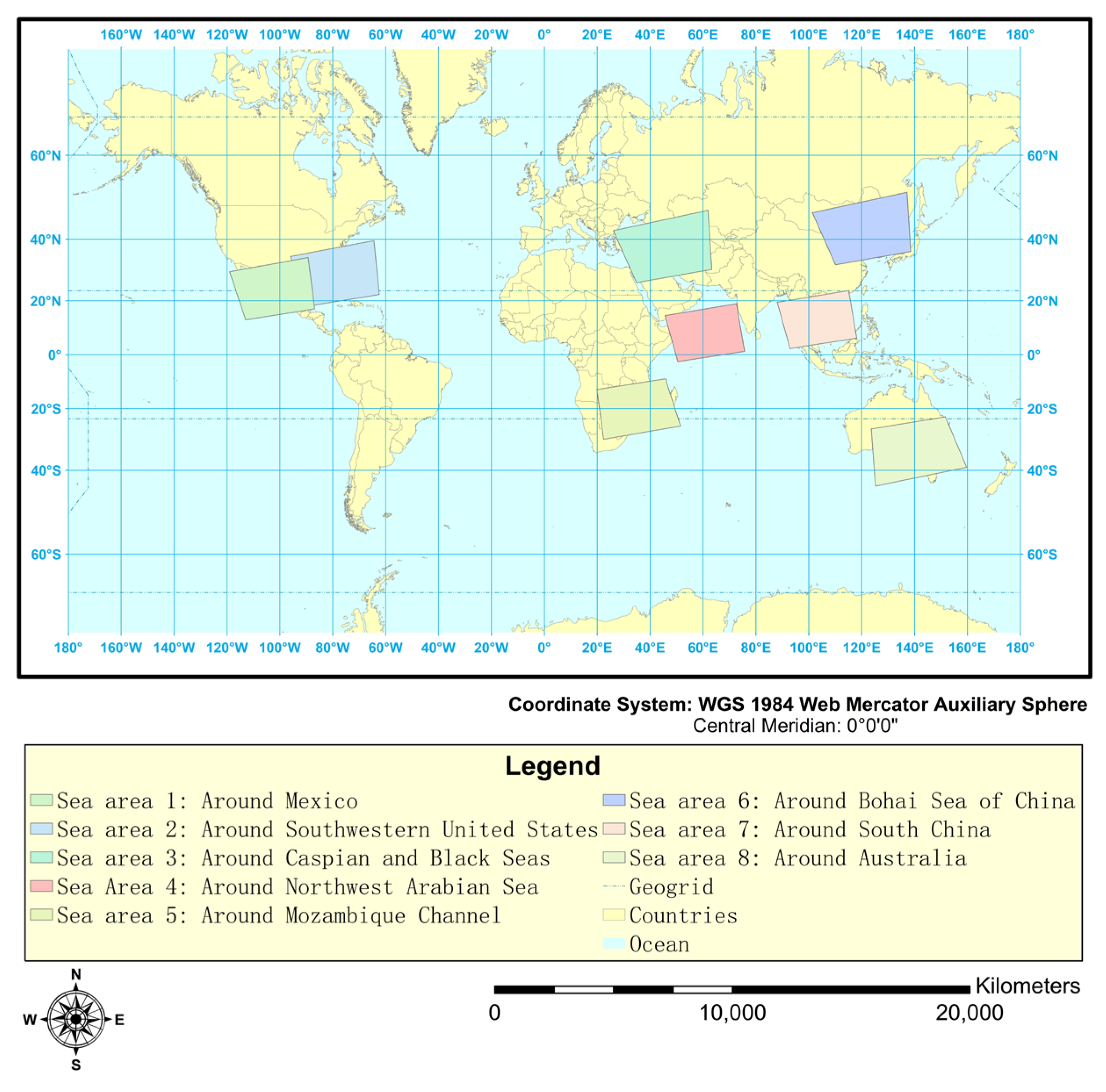
2.1. Data and Study Area

2.1.1. FY-3D/MERSI-II Satellite Data

MERSI-II is the second generation of optical imaging payload with improved performance carried out by the FY-3D satellite since it was launched in November 2017. It integrates two imaging instruments from the original FY-3 satellite—the visible and infrared radiometer (VIRR) and the first-generation MERSI function. FY-3D MERSI-II has a total of 25 bands, and it has 6 channels in the visible light band, 10 channels in the visible light/near-infrared band, 3 channels in the short-wave infrared band, and 6 channels in the medium- and long-wave infrared band [30,31]. The instrument can obtain abundant Earth–gas radiation images at the same time. In this study, 8 bands of visible light and near-infrared band are selected for AC. The information for these bands is listed in Table 1. The National Satellite Meteorological Center (NSMC) of China provides L1 data, and after calibration correction, they are converted into apparent reflectance.

2.1.2. Global/Regional Assimilation and Prediction Enhanced System (GRAPES) Data

The CMA independently developed the Global and Regional Assimilation and Prediction System (GRAPES), which is widely used for numerical weather and climate forecasting. GRAPES has three major systems, including the Global Medium-Range Numerical Forecast System (GRAPES-GFS), the Regional Mesoscale Forecast System (GRAPES-MESO), and the Typhoon Model Forecast System (GRAPES-TYM) numerical weather forecasting systems with independent intellectual property rights in China. At present, it provides the highest horizontal resolution of 0.25° × 0.25°, with 60 vertical layers [32]. GRAPES also has a complete physical process framework for weather forecasting and has been formally applied to the field of weather forecasting in China. Seven forecast data of satellite areas across similar times are applied as the input source of the algorithm to participate in the calculation (Table 2). In this study, we use the GRAPES data as the meteorological ancillary data in the SIRAW algorithm.

2.1.3. AERONET-OC In Situ Measurement Data

The AErosol RObotic NETwork (AERONET) is a worldwide system of autonomous solar photometers set up in the early 1990s to support atmospheric research at various scales by standardized measurements of direct Sun and sky radiation [33]. AERONET has played an important role in the study of the optical properties of aerosols, the creation of global climate aerosols, and the validation of atmospheric remote sensing products. Since 2006, the network has been extended by a new component called AERONET ocean color (AERONET-OC), which provides additional capacity for identifying ocean WLR, and the data are collected by an improved solar photometer installed on a fixed offshore platform.
Data observation is based on the CIMEL CE-318 automated Sun photometers. It shows the ability to perform marine radiometric measurements for determining WLR in addition to the regular measurements for retrieving aerosol optical properties. A system based on the Sea-Viewing Wide Field-of-View Sensor (SeaWiFS) and Photometer Revision for Incident Surface Measurements (SeaPRISM) performs multiple sky and sea radiance measurements at given viewing and azimuth angles at eight center wavelengths in the 412–1020 nm spectral range [34,35].
The newest version 3 level 2.0 data are obtained to validate the retrieved SIRAW WLR, because after completing pre- and post-field calibration with differences smaller than 5%, automatic cloud removal, and manual inspection, they have been fully quality-controlled. Compared to the same sea area as shown in the study area map, the 2021 whole-year WLR data are downloaded to carry out the validation (Figure 1).

2.1.4. Visible Infrared Imaging Radiometer Suite (VIIRS) OC Satellite Data

In October 2011, the Suomi-NPP US watercolor satellite equipped with VIIRS sensors was successfully launched, which is the mainstream of current international ocean color observation. The Suomi-NPP orbits the Earth at an altitude of approximately 834 km and completes a single orbit in approximately 101 min. It completes daily global coverage after about 14 orbital flights. VIIRS is one of 5 sensors carried by Suomi-NPP for Earth observation. It collects visible light and infrared bands in the 0.4~12 μm range and combines some of the key capacities of traditional instruments, such as Medium Resolution Imaging Spectroradiometer (MODIS), Advanced Very High-Resolution Radiometer (AVHRR), and Operational Line Scanning System (OLS) [36]. The open-access VIIRS WLR product covers from 410 nm to 671 nm, so we chose a similar MERSI-II band to carry out the comparison. Therefore, this study only shows 5 bands’ comparison results among 412 nm, 443 nm, 490 nm, 555 nm, and 670 nm. The description of these wavelengths is shown in Table 3.

2.1.5. Match-Up Procedure

In this study, data from 2021 from the ground-based observation station AERONET-OC are selected to carry out verification work. In the model retrieval scheme, we select the data without the Sun glint contamination when the reflected solar angle is over 36.0 degrees in the clear sky. The cloudy pixels are excluded from the validation when the standard deviation of 550 nm apparent reflectance within 5 × 5 pixels is less than 0.0025, and the standard deviation of 490 nm apparent reflectance is less than 0.4. In addition, the data of ground observation and satellite transit time difference within 1.5 h are selected to ensure the time matching of the two kinds of data. The average WLR of 3 × 3 pixels is selected as the verification data of satellite inversion. We compared the relative error (RE) and root mean square error (RMSE) to analyze the comparison between SIRAW and ground-based measurement data.
For the inter-comparison with VIIRS, satellite images are down-sampled to 4 km, excluding pixels where the viewing and solar zenith angles exceed 60 and 75 degrees, respectively. Spatial and temporal matching of the SIRAW retrieval and VIIRS WLR are based on the same locations and similar overpass times. VIIRS- and SIRAW-retrieved WLRs are converted to R r s as Equation (1). All samples are compared in this research. The difference is quantified by the following statistical parameters: the coefficient of determination (R), the RMSE, the bias, the mean bias error (MBE), MRB represents bias/mean (VIIRS), and r_RMSE stands for RMSE/mean (VIIRS).
R r s = n L w F 0
To compare the spatial distribution of retrieved AOT and WLR from MERSI, we make an inter-comparison with those of VIIRS in different oceanic areas. There are 8 coastal sea areas chosen for the inter-comparison in the global scale on 11 March 2020, around Mexico, the southwestern United States, the Caspian and Black Seas, the northwest Arabian Sea, the Mozambique Channel, the Bohai Sea of China, south China, and Australia, of which the spatial region is shown in Figure 2. The FY-3D/MERSI-II L1 5 min 1 km orbital data images of these 8 turbidity CASE-II water bodies are selected as the input data. The area of these images depends on the orbital data obtained by the satellite at the transit time there. In addition, to investigate the effects of calibration coefficients on the retrieval, we conduct the inter-comparison of retrieved WLR between MERSI and VIIRS around the South China Sea (see Figure 3), where the high-value condition of WLR occurred according to the VIIRS observation on 30 August 2022. The research flowchart is shown in Figure 4 below.

2.2. Methods

The SIRAW method was jointly constructed by Shi et al. [9,20,29]. It has been applied to the Japan Aerospace Exploration Agency (JAXA) scientific research platform, Greenhouse gases Observing SATellite-2 (GOSAT-2), and Global Change Observation Mission-Climate (GCOM-C) and proved to have a high ability to retrieve the aerosols and WLR [9,29,37,38].
The forward radiation calculation was performed by the improved vector radiative transfer model named Pstar [9,20,37,39]. In this model, a three-component bio-optical module was used for the turbid waters and a full-physical WLR calculation scheme was developed [20]. Pstar is a vector-coupled atmosphere–ocean RT model for forward RT simulation combined with discrete ordinate and matrix operator methods proposed by Ota et al. [39], which inherits from the classic Nakajima–Tanaka scheme [40,41,42,43]. The result has proved to be precise in simulating radiation in atmospheric and ocean systems [44,45]. The source function term in the RTE increases the effect of direct solar beams reflected or transmitted by the ocean surface, as shown below in Equation (2):
μ d L ( τ ; μ , φ ) d τ = L τ ; μ , φ + ω 1 1 0 2 π P μ , φ ; μ , φ L τ ; μ , φ d φ d μ + S + 1 ω B ( τ )
where τ is the optical depth measured from the top of the atmosphere (TOA), μ is the cosine of the viewing zenith angle, φ is the azimuth angle. The scalar ω represents the single scattering albedo, which is defined as the ratio of the scattering coefficient to the extinction coefficient. Additionally, P is the phase matrix, and S is the source function for single scattering. It is defined differently in atmospheric and oceanic systems. These two systems’ formulas are listed below in Equation (3) and Equation (4), respectively.
S = ω P μ , φ ; μ 0 , φ 0 F 0 e τ μ 0 + ω P μ , φ ; μ 0 , φ 0 R s μ 0 , φ 0 ; μ 0 , φ 0 F 0 e 2 r a τ μ 0
S = ω μ 0 μ ~ 0 P μ , φ ; μ 0 , φ 0 T s μ ~ 0 , φ 0 ; μ 0 , φ 0 F 0 e τ a μ 0 e τ τ a μ ~ 0
where F 0 is the solar flux vector, τ a is the optical thickness of the whole atmosphere, and μ ~ 0 is the refraction cosine of the solar zenith angle in the ocean. R s and T s represent the reflection matrix and transmission matrix of the sea surface, respectively. These two parameters can be calculated using Nakajima and Tanaka’s [43] algorithm for rough ocean surfaces.
In the inhomogeneous atmospheric and oceanic layers, the solutions of RTE are computed based on the discrete ordinate and matrix operator methods [38], as well as a highly accurate and efficient truncation method [41]. Pstar has been shown to have good accuracy in simulating radiation processes in both the atmosphere and the ocean [20]. In the atmosphere system, three aerosol types, including fine, sea salt, and dust particles, are considered. In addition, the fine particles are assumed to be an internal mixture of water-soluble, soot, and dust-like particles. In the ocean system, a three-component bio-optical ocean module is developed to simulate the inherent optical properties of the water constituent concentration (WCC), which includes chlorophyll-a (CHL-a), suspended sediment (Ss), and colored dissolved organic matter (CDOM). The ocean surface is modeled using the Nakajima and Tanaka scheme [43], of which the reflection and transmission matrix consider the effect of wind-generated waves on the solar radiation transfer in the atmosphere–ocean system.
The SIRAW algorithm uses the optimal estimation theory to construct the inversion module. In non-linear atmospheric and oceanic systems, the measurement vector y , such as the observed radiance or reflectivity, can be divided into the expression of the forward radiative transfer model F x and error ε which consists of the measurement error and the model error (Equation (5)). Then, under the condition of prior information constraints, the maximum a posteriori optimization method is used to minimize the cost function in an iterative way (Equation (6)).
y = F x + ε
x i + 1 = x i + K i T S ε 1 K i + S a 1 1 K i T S ε 1 y F x i S a 1 x i x a
where x i is the state vector to be retrieved at the i iteration, which includes the AOTs of fine, sea salt, and dust particles, soot fraction of fine particles, Chl-a, Ss, and CDOM; x a is the prior state vector, S ε is the measurement error covariance matrix, S a is the prior state value determined error covariance matrix; K denotes the Jacobian matrix or weighting function, which is derived from the forward model to the state vector, and can be defined as the equation K = ∂F(x)/ ∂x.
To improve the calculation efficiency of the SIRAW algorithm, a radiative transfer neural network (NN) solver is constructed to perform the forward radiation calculation. In this study, we randomly generated a huge training dataset based on the coupled atmosphere–ocean radiative transfer model. The training dataset covers various atmospheric and oceanic parameters, including AOT of fine particles, AOT of sea salt, AOT of dust, soot fraction, Chla, Ss, CDOM, sea level pressure, 10 m height wind speed from ocean surface, total column ozone, relative humidity, solar zenith angle, satellite zenith angle, relative azimuth angle, and simulated satellite reflectance and WLR at the wavelength of MERSI OC channels from 412 nm to 865 nm. To further improve the learning efficiency of the NN solver, we use an advanced self-adoption varied learning scheme developed by Shi et al. [29] to adjust the learning rate of each neuron.
Then, the simulated apparent reflectance of the top atmosphere is solved by using the deep-learning-based fast radiative transfer solver described above. Based on the Bayesian optimal estimation theory, the relevant parameter information is constantly optimized through several iterations. The error of the apparent reflectance of satellite observation and NN solver simulation is minimized, and the retrieved state vector is determined. Finally, the WLR is calculated based on the retrieved atmospheric and oceanic parameters through the NN radiative transfer solver.
In the full physical technology model of WLR and underwater light field, the algorithm from Shi et al. [9] is used to solve L w . The equations are shown below in Equation (7):
L w λ ; μ , φ ; C h l , S s , a y 440 , A O T , W i n d = m = 0 M 1 L W m ( λ ; μ ; C h l , S s , a y 440 , A O T , W i n d ) cos m φ π ( 1 + δ 0 m )
where λ is the wavelength, δ 0 m is Kronecker’s delta; μ is the cosine of the viewing zenith angle and φ is the cosine of the relative azimuth angle. [Chl], Ss, and a y (440) represent the concentrations of chlorophyll, sediment, and absorption coefficient of CDOM at 440 nm, respectively. L w in a single direction can be decomposed into Equations (8) and (9).
L W m λ ; μ ; C h l , S s , a y 440 , A O T , W i n d = i = 1 N s L u m λ ; τ 0 ; μ i ; C h l , S s , a y 440 , A O T , W i n d T m λ ; μ , μ i
T m λ ; μ , μ i = 1 μ i μ i 1 2 μ i + 1 2 μ d μ 0 2 π T λ ; μ , μ ; φ cos m φ   d φ
T λ ; μ , μ ; φ is the rough sea surface’s diffuse transmission function and is related to the incident zenith angle and the exit zenith angle μ and μ above and below the sea surface. T m is the M-order Fourier component of the diffuse transmission matrix of the rough ocean surface. According to the sea surface model of Nakajima et al. [43], T λ ; μ , μ ; φ can be derived from model inversion wind speed parameters. Finally, obtaining the value of L w , after parameter derivation, the W L R data of 412 nm, 443 nm, 490 nm, 555 nm, and 670 nm are generated.
L w converts into W L R in Equation (10):
W L R λ ; C h l , S s , a y 440 = d 0 d 2 L w { λ ; N a d i r ; C h l , S s , a y 440 , A O T , W i n d } E d 0 + λ F 0 λ
where d 0 is the Earth–Sun average distance, F 0 is solar irradiance, d is the Earth–Sun distance at the time of measurement, E d 0 + is the downward solar irradiance over the sea.
SIRAW makes up for the shortcomings of the large uncertainty of traditional coastal region AC schemes in a complex environment. By constructing a fast coupled atmosphere–ocean radiation transmission model and combining it with the optimal estimation theory, the coastal region AC method with multi-parameter synchronous inversion is developed to meet the physical mechanism requirements of the combined influence of atmospheric and ocean parameters on satellite spectra. At the same time, it solves the bottleneck problem that the calculation efficiency of traditional optimal estimation theory is too low to meet the demand of the practical application. In addition, the WLR is calculated by using the fast RT solver, avoiding the inefficient problem based on the traditional physical-based optimal estimation (OE) method, which further avoids the negative phenomenon of the short-wave WLR retrieved by the traditional algorithm.

3. Results

3.1. Validation of NN Radiative Transfer Solver

In the SIRAW algorithm, the retrieved AOT and WLR are determined based on the optimal estimation method in an iterative way, as shown in Equations (5)–(10). Compared with the traditional LUT method, the optimal estimation method is more feasible in the retrieval of multiple parameters from multiple observation information, which has been commonly used in the remote sensing of aerosols, gases, ocean color, etc. However, studies indicate that the calculation efficiency of the optimal estimation method is much lower than that of the LUT-based method [21] due to the frequent operation of forward radiative transfer calculation during the retrieval, which constrains its performance in the operational process of satellite imager data.
In this study, we develop an NN radiative transfer solver to replace the coupled radiative transfer model for the forward radiation calculation. Compared with the LUT method, the NN technique is more flexible and efficient for forward calculation when multiple input parameters are varied coordinately, particularly in the non-linear system. In contrast, it has to take a huge calculation loading in the LUT method since a high-dimensional LUT volume needs to be constructed to make the LUT-based radiation calculation unpractical.
To develop the NN solver used in the AC of FY-3/MERSI, 2 million simulated datasets are produced based on the full physical radiative transfer model, combined with the developed adaptive learning rate neural network algorithm. We constructed an individual NN solver for each OC channel of MERSI. Each NN solver has one input layer, three hidden layers, and one output layer with 14, 120, 80, 50, and 1 neuron in each layer. We randomly split the entire prior dataset and divided it into training, test, and validation data in an 8:1:1 ratio. A large amount of training data are used to iteratively optimize the weight and bias of the neural network. At the same time, test data are used to control the reliability of the simulation parameters of the neural network to avoid overfitting in the training process. Finally, the optimal NN solver is obtained based on the validation data.
Figure 5 shows the accuracy of the NN radiative transfer solver validated by the full-physical coupled radiative transfer model, i.e., Pstar. Results show that a very good consistency between the NN solver and RT model is identified. The relative errors of simulated TOA reflectance below 600 nm are generally less than 0.5%, and those above 600 nm are less than 0.7%, which are significantly lower than the uncertainties of MERSI observation. As for the calculation efficiency, the running speed of a single pixel is less than 0.00002 s, which greatly improves the radiation calculation efficiency. In comparison, the calculation time of the original full physical radiation model is about 3.9 s. Based on the NN solver, we adopted it in the SIRAW algorithm for the forward radiation calculation, i.e., F x i in Equation (5), during each iteration.

3.2. Validation with AERONET-OC

Based on the developed NN radiative transfer solver for the forward radiation calculation, combined with the MERSI-measured observation spectrum, the inversion results of the SIRAW are validated with the ground-based observation network of AERONET-OC in different coastal regions around the world in 2021 (see Figure 6). This validation involves 412, 443, 490, and 555 nm, and the number of matching verification points is 30. The reason for choosing validated wavelengths from 412~555 nm is that those bands are mostly used in the retrieval of chlorophyll concentration, which is the most significant parameter in the OC. In addition, observation of WLR from AERONET-OC also indicates a typically below 5% uncertainty at 412~551 nm and approximately 8% uncertainty at 667 nm [46]. As can be seen from Figure 6, there is generally good consistency of WLR in each channel between MERSI and in situ measurement. In detail, 490 nm showed the best WLR retrieval results with a deviation of 23% and an RMSE of 0.191. The inversion results at 412 nm and 443 nm were also good, with deviations of about 28% and RMSE of 0.188 and 0.204, respectively, while a slight underestimation is identified in the high-value condition. To sum up, the results show that the inversion error Re of WLR below 600 nm is generally within 35%. There is no extreme deviation in the SIRAW inversion results compared with AERONET-OC, with a generally good agreement with the observed values, which support the availability of SIRAW in the retrieval of aerosols and WLR in coastal water and performance of MERSI for monitoring the aerosols and OC signals.

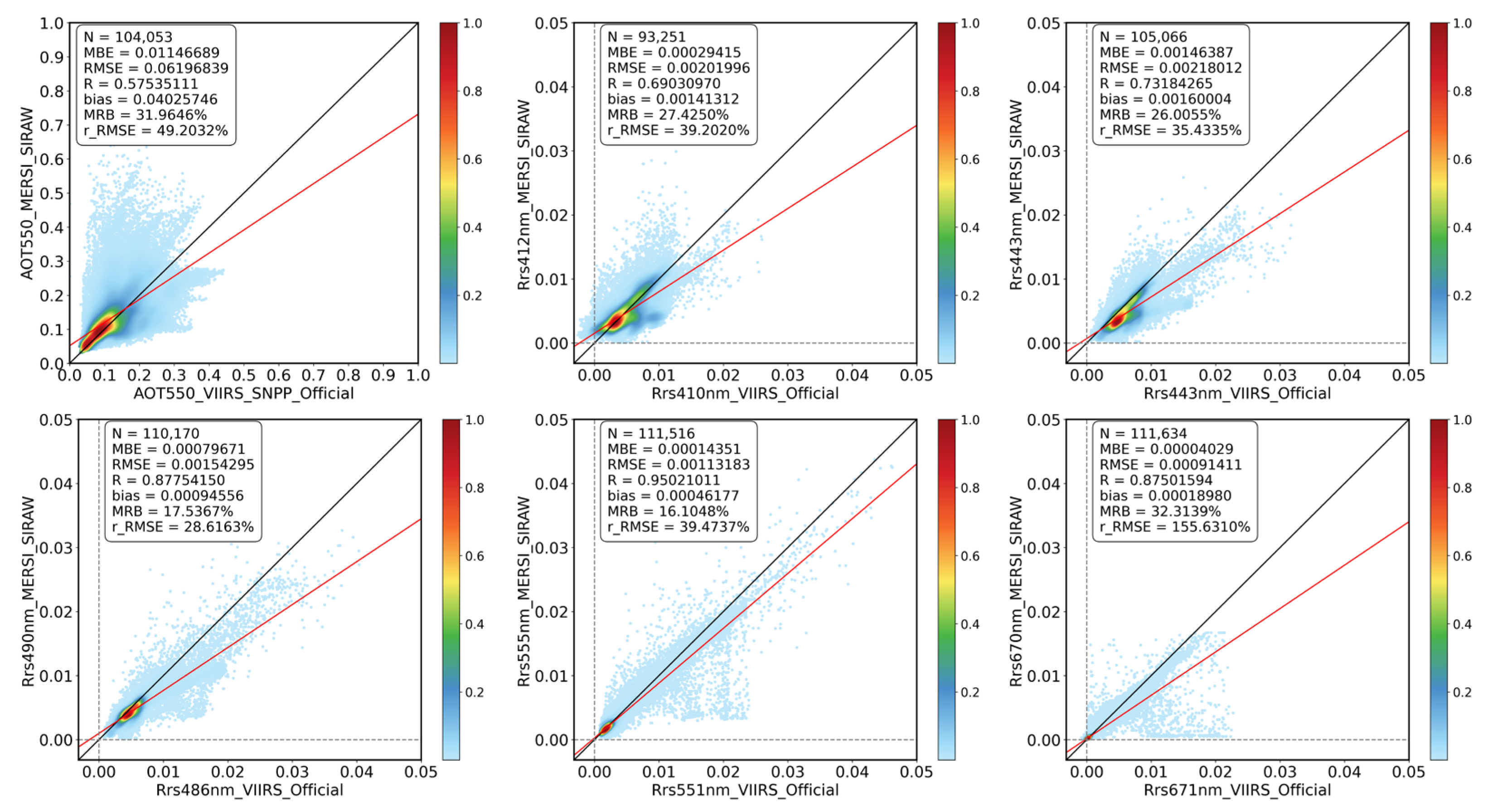
3.3. Inter-Comparison with VIIRS Images

Figure 7 shows the verification and inter-comparison results of SIRAW-retrieved AOT and WLR with VIIRS official products and shows the two types of data have a strong spatial consistency. The traditional algorithm used for the VIIRS official product still presents the phenomenon of “over-correction”, and many WLR values less than 0 are shown in the scatter plot, i.e., 410 nm and 671 nm of VIIRS. On the contrary, the SIRAW effectively avoids this phenomenon, and there are no WLR values less than 0 in the result. AOT inversion in 550 nm has a deviation of about 0.04 compared with VIIRS. On the basis of this precision, we invert the WLR and, additionally, further solve the R r s to make the comparison. The result shows that the SIRAW-retrieved R r s strongly correlates with VIIRS R r s among eight typical Case-II water regions, and the best matching results appear at bands 490 nm and 555 nm. Of which, the fitting results of 555 nm are the best, with the highest correlation at 0.95. The RMSEs of 490 nm, 555 nm, and 670 nm are around 0.001, showing only minimal data bias from the validated data. For the remaining two bands, RMSE is around 0.002, and this inversion result still shows a relatively reliable data statement. From the data distribution of the scatter plot, it can be seen that the scatter distribution of 443 nm, 490 nm, and 555 nm bands is more concentrated. On the whole, the WLR retrieval capability of the SIRAW algorithm is close to that of VIIRS retrieval in typical near-shore muddy waters around the world, and the spatial state distribution of the two data is similar. Inter-comparison of R r s at the near-ultraviolet channel, i.e., 412 nm of MERSI and 410 nm of VIIRS, indicates that there are still negative R r s values of the VIIRS official product. In comparison, the SIRAW-based MERSI R r s product is promising to avoid this phenomenon. The existence of negative R r s on band 443 nm further confirms the difficulties of the AC algorithm in the coastal areas due to the overestimation of aerosols.

4. Discussion

This section discusses the influence of the radiometric calibration coefficient correction for the FY-3D/MERSI visible light bands on the accuracy of SIRAW WLR inversion.
To obtain an accurate oceancolor signal, the detection ability of the sensor needs to reach a very high level. Due to the detection sensitivity of the traditional satellite sensor not being enough, auxiliary optical remote sensing load calibration needs to be carried out. In the field of water constituent inversion, the uncertainty of TOA reflectance is required to be better than 0.5%, and to achieve this accuracy level, the contribution of uncertainty caused by polarization, stray light, response non-linearity, and other factors needs to be controlled in the order of 0.1% [47]. Radiometric calibration mainly refers to the process of converting the remote sensing values observed from the satellite sensor into absolute values of physical quantities. Outside the atmosphere, the irradiance of the Sun can be identified as a constant, so the Sun can be selected as the reference light source to carry out radiometric calibration of the space-borne imaging spectrometer through the solar calibration system, that is, on-board calibration, such as MODIS data. The radiometric calibration coefficients for this type of data are provided in the header file, the same as FY-3D.
The FY-3D satellite launched on 15 November 2017, and it has been in operation in orbit for more than 5 years. NSMC provides the MERSI-II L1 calibration coefficients, which were calibrated in January 2019. Due to the influence of instrument attenuation and atmospheric environment factors, the calibration ability of calibration parameters deteriorates, which makes the radiation correction deviation and the product accuracy not as high as that of the satellite launch [48]. It is necessary to evaluate the absolute radiometric calibration accuracy of MERSI-II’s visible light bands for the purpose of the possible influences of calibration uncertainties on WLR products.

4.1. Calibration Coefficient Correction

Normal methods of atmospheric–ocean AC use visible light and near-infrared bands. For MERSI-II, 412 nm to 865 nm bands are designed to study ocean water color, plankton, and biogeochemicals. Section 3 shows the results of the SIRAW algorithm on the FY-3D/MERSI-II sensor in early 2020, and demonstrates that SIRAW had a better performance in eliminating the effect of aerosol scattering to obtain a more accurate watercolor signal. However, in the test of the South China Sea WLR retrieval work in August 2022 (the study area is shown in Figure 3), it is found that the accuracy of the algorithm has attenuated recently, which probably depends to a certain extent on the attenuation of the MERSI-II blue light channel, when considering that lots of research proved that 412 nm and 443 nm bands are confirmed to damp gradually [49,50,51]. In order to explore the relatively poor inversion accuracy results and the recent attenuation of verification results of these channels, calibration correction of visible light band coefficients was carried out for the bands 412 nm and 443 nm of FY-3D.
Excluding the reason of the method itself, the state of MERSI-II L1 data in different time periods will also affect the reliability of the SIRAW. The instrument’s radiation detection error will propagate with the extrapolation calculation and directly affect the inversion result. In order to ensure the accuracy of remote sensing data, radiometric calibration of satellite-borne sensors should be carried out regularly. Therefore, we carried out the accuracy check of the calibration coefficients of the MERSI-II L1 data. It can be seen from Table 4 that the calibration accuracy at 412 nm decreases sharply from 2.35% to 19.32%, and the calibration accuracy at 443 nm decreases from 1.86% to 11.31%. Both blue bands show at least 10% scaling accuracy attenuation. In order to verify whether the algorithm accuracy attenuation is caused by the MERSI L1 data calibration accuracy reduction, the subsequent re-calibration is carried out and the verification accuracy is compared.
The integrated method for on-orbit-wide dynamic vicarious calibration [52] is used for FY-3D/MERSI-II reflective solar bands. This method integrates a variety of alternative schemes that do not rely on ground synchronization measurement and uses the multi-level reflectance characteristics of the calibrated samples by each scheme to realize the radiometric calibration of remote sensors in a wide dynamic range. The calibration samples of each scheme were fused with equal weights by the piecewise average method, and the final calibration coefficient was obtained by weighted fitting regression based on the fused samples. The non-linear features were corrected using the quadratic coefficients analyzed in outdoor calibration experiments before launch, and the calibration slope and intercept were calculated in orbit.
The coefficient changes are shown in Table 5.

4.2. Inversion of Water-Leaving Radiance Based on FY-3D Data

The scatter density plots below (Figure 8 and Figure 9) show the comparison of R r s retrieval results using old and re-calibrated coefficients, respectively, and present the accuracy improvement of the AC work in the South China Sea area before and after correction. Compared to the output AOT and 5-band retrieval WLR, the correlation of all channels is increased significantly, and the RMSE shows an obvious decreasing trend. Table 6 shows that each accuracy index has been greatly improved in each band. This proves that the inverted WLR after re-calibration is more consistent with VIIRS than before, and the re-calibrated coefficients are more accurate. Figure 10 is the R r s spatial distribution map of SIRAW inversion, which shows that the spatial state of the inverse performance of the new calibration coefficients is closer to VIIRS products. All indicators revealed that WLR derived from the optimized calibration coefficients has obvious correlation improvement and error reduction compared with VIIRS’s official OC product. In addition, although only 412 nm and 443 nm were calibrated, the accuracy and error have been significantly enhanced and reduced for all channels of the WLR. The results confirm that re-calibrated coefficients can improve retrieval accuracy and that the accurate blue light band calibration coefficients of FY-3D/MERSI can effectively avoid the inversion error caused by error transmission.

5. Conclusions

This article presents a simultaneous retrieval algorithm of SIRAW and utilizes it in the FY3D/MERSI-II bands 8~15 to retrieve aerosols and WLR. The SIRAW algorithm uses a neural network-based radiative transfer solver and Bayesian optimal estimation theory, considering the coupled radiation process in the atmosphere–ocean system. After validation and inter-comparison with the ground-based measurement data from AERONET-OC and VIIRS WLR products, it is confirmed that the retrieved aerosols and WLR data have high accuracy and reliable results in different Case-II turbid ocean areas. The SIRAW algorithm avoids the negative phenomenon of the WLR retrieval that classic AC algorithms have, even for the current VIIRS OC products. The application of SIRAW in FY-3D/MERSI-II is promising for estimating the influence of aerosol scattering on the satellite signal by providing reliable aerosol and WLR. At the same time, this paper takes the South China Sea as an example to demonstrate the sensitivity of radiometric calibration to reduce error transmission and obtain accurate watercolor signals in AC work. The optimization of the visible light calibration coefficients of 412 and 443 nm bands has a significant improvement in the accuracy of each band in the WLR inversion for the MERSI sensor. This result also gives strong evidence to prove that the correction of the blue band calibration coefficients can reduce the error transmission via inversion, and proves the radiometric calibration is of great significance for the SIRAW inversion of aerosol and WLR data.
In the future, orbit-by-orbit and day-by-day WLR data will be regularly produced by SIRAW, and these datasets will continue to be validated and inter-compared with AERONET-OC in situ measurement data and VIIRS satellite product data, respectively. We will continue to pay attention to the stability of the inversion of SIRAW on the FY-3/MERSI series data, check and evaluate the state of the algorithm, and calibrate MERSI on the aerosols and OC detection.

Author Contributions

Conceptualization, X.Z. and C.S.; methodology, C.S., X.H. and H.L.; validation, X.Z., C.S., Y.S., L.W., C.T. and Z.Z.; investigation, X.Z.; writing—original draft preparation, X.Z.; writing—review and editing, X.Z., C.S., Y.S., S.Y., L.C. and N.X.; project administration, L.C. and N.X.; funding acquisition, L.C. All authors have read and agreed to the published version of the manuscript.

Funding

This work is supported by the National Key Technology Research and Development Program of China (2021YFB3901000 and 2021YFB3901005) and supported by the Youth Innovation Team of the “Fengyun Satellite Remote Sensing Product Verification” (CMA2023QN12) of the China Meteorological Administration and funding by Fengyun Application Pioneering Project (FY-APP-2022.0304). This article is also supported by the open fund of the State Key Laboratory of Satellite Ocean Environment Dynamics, Second Institute of Oceanography, MNR (No. QNHX2207) and supported by the National Natural Science Foundation of China (grant number 42275145). The Joint Research Project for Meteorological Capacity Improvement (No.2023QN083) also supported this article.

Data Availability Statement

The FY-3D/MERSI data and meteorological data used in this article are from the National Satellite Meteorological Center (National Center for Space Weather). The validation data of AERONET-OC and VIIRS were downloaded from https://aeronet.gsfc.nasa.gov/new_web/download_all_v3_lwn.html (accessed on 30 August 2023) and ftp://ftp.star.nesdis.noaa.gov/pub/socd1/mecb/coastwatch/viirs/science/L3/global/nlw (accessed on 30 August 2023), respectively.

Acknowledgments

Thanks to AERONET-OC and VIIRS for providing valuable comparative data for this article. The authors would like to thank the anonymous reviewers for their constructive comments.

Conflicts of Interest

Author Zhihua Zhang was employed by the Beijing Huayun ShineTek Technologies Co. The remaining authors declare that the research was conducted in the absence of any commercial or financial relationships that could be construed as a potential conflict of interest.

References

  1. Platt, T.; Sathyendranath, S.; Forget, M.H.; White, G.N.; Caverhill, C.; Bouman, H.; Devred, E.; Son, S.H. Operational estimation of primary production at large geographical scales. Remote Sens. Environ. 2008, 112, 3437–3448. [Google Scholar] [CrossRef]
  2. Kirk, J.T.O. Light and Photosynthesis in Aquatic Ecosystems, 3rd ed.; Cambridge University Press: Cambridge, UK, 2010; pp. 1–651. [Google Scholar] [CrossRef]
  3. Jun, C.; Jun, F.; Jihong, S. Influences of geometric correction on the accuracy of dark pixel atmospheric correction algorithm and water leaving irradiance retrieval:a case study of Lake Taihu. J. Lake Sci. 2011, 23, 89–94. [Google Scholar] [CrossRef]
  4. Gordon, H.R. Removal of atmospheric effects from satellite imagery of the oceans. Appl. Opt. 1978, 17, 1631–1636. [Google Scholar] [CrossRef] [PubMed]
  5. Gordon, H.R.; Wang, M. Retrieval of water-leaving radiance and aerosol optical thickness over the oceans with SeaWiFS: A preliminary algorithm. Appl. Opt. 1994, 33, 443–452. [Google Scholar] [CrossRef] [PubMed]
  6. Ahmad, Z.; Montes, M.J.; Davis, C.O.; Gao, B.-C. Atmospheric correction algorithm for hyperspectral remote sensing of ocean color from space. Appl. Opt. 2000, 39, 887–896. [Google Scholar] [CrossRef]
  7. Antoine, D.; Morel, A. A multiple scattering algorithm for atmospheric correction of remotely sensed ocean colour (MERIS instrument): Principle and implementation for atmospheres carrying various aerosols including absorbing ones. Int. J. Remote Sens. 1999, 20, 1875–1916. [Google Scholar] [CrossRef]
  8. Fukushima, H.; Higurashi, A.; Mitomi, Y.; Nakajima, T.; Noguchi, T.; Tanaka, T.; Toratani, M. Correction of atmospheric effect on ADEOS/OCTS ocean color data: Algorithm description and evaluation of its performance. J. Oceanogr. 1998, 54, 417–430. [Google Scholar] [CrossRef]
  9. Shi, C.; Nakajima, T. Simultaneous determination of aerosol optical thickness and water-leaving radiance from multispectral measurements in coastal waters. Atmos. Chem. Phys. 2018, 18, 3865–3884. [Google Scholar] [CrossRef]
  10. He, X.; Pan, D.; Mao, Z. Atmospheric correction of Sea WiFS imagery for turbid coastal and inland waters. Acta Oceanol. Sin. 2004, 23, 609–615. [Google Scholar] [CrossRef]
  11. He, X.; Bai, Y.; Pan, D.; Tang, J.; Wang, D. Atmospheric correction of satellite ocean color imagery using the ultraviolet wavelength for highly turbid waters. Opt. Express 2012, 20, 20754–20770. [Google Scholar] [CrossRef]
  12. Wang, M.; Shi, W.; Esaias, W.E.; Abbott, M.R.; Barton, I.; Brown, O.B.; Campbell, J.W.; Carder, K.L.; Clark, D.K.; Evans, R.L.; et al. The NIR-SWIR combined atmospheric correction approach for MODIS ocean color data processing. Opt. Express 2007, 15, 15722–15733. [Google Scholar] [CrossRef] [PubMed]
  13. Hu, C.; Carder, K.L.; Muller-Karger, F.E. Atmospheric Correction of SeaWiFS Imagery over Turbid Coastal Waters: A Practical Method. Remote Sens. Environ. 2000, 74, 195–206. [Google Scholar] [CrossRef]
  14. Bailey, S.W.; Franz, B.A.; Werdell, P.J. Estimation of near-infrared water-leaving reflectance for satellite ocean color data processing. Opt. Express 2010, 18, 7521–7527. [Google Scholar] [CrossRef]
  15. Moore, G.F.; Aiken, J.; Lavender, S.J. The atmospheric correction of water colour and the quantitative retrieval of suspended particulate matter in Case II waters: Application to MERIS. Int. J. Remote Sens. 2010, 20, 1713–1733. [Google Scholar] [CrossRef]
  16. Siegel, D.A.; Wang, M.; Maritorena, S.; Robinson, W. Atmospheric correction of satellite ocean color imagery: The black pixel assumption. Appl. Opt. 2000, 39, 3582–3591. [Google Scholar] [CrossRef] [PubMed]
  17. Chomko, R.M.; Gordon, H.R. Atmospheric correction of ocean color imagery: Use of the junge power-law aerosol size distribution with variable refractive index to handle aerosol absorption. Appl. Opt. 1998, 37, 5560–5572. [Google Scholar] [CrossRef] [PubMed]
  18. Kuchinke, C.P.; Gordon, H.R.; Franz, B.A. Spectral optimization for constituent retrieval in Case 2 waters I: Implementation and performance. Remote Sens. Environ. 2009, 113, 571–587. [Google Scholar] [CrossRef]
  19. Land, P.E.; Haigh, J.D. Atmospheric correction over case 2 waters with an iterative fitting algorithm: Relative humidity effects. Appl. Opt. 1997, 36, 9448–9455. [Google Scholar] [CrossRef]
  20. Shi, C.; Nakajima, T.; Hashimoto, M. Simultaneous retrieval of aerosol optical thickness and chlorophyll concentration from multiwavelength measurement over east China sea. J. Geophys. Res. 2016, 121, 14,084–14,101. [Google Scholar] [CrossRef]
  21. Frouin, R.J.; Franz, B.A.; Ibrahim, A.; Knobelspiesse, K.; Ahmad, Z.; Cairns, B.; Chowdhary, J.; Dierssen, H.M.; Tan, J.; Dubovik, O.; et al. Atmospheric Correction of Satellite Ocean-Color Imagery during the PACE Era. Front. Earth Sci. 2019, 7, 145. [Google Scholar] [CrossRef]
  22. Brajard, J.; Jamet, C.; Moulin, C.; Thiria, S. Use of a neuro-variational inversion for retrieving oceanic and atmospheric constituents from satellite ocean colour sensor: Application to absorbing aerosols. Neural Netw. 2006, 19, 178–185. [Google Scholar] [CrossRef] [PubMed]
  23. Jamet, C.; Thiria, S.; Moulin, C.; Crepon, M. Use of a Neurovariational Inversion for Retrieving Oceanic and Atmospheric Constituents from Ocean Color Imagery: A Feasibility Study. J. Atmos. Ocean. Technol. 2005, 22, 460–475. [Google Scholar] [CrossRef]
  24. Schroeder, T.; Behnert, I.; Schaale, M.; Fischer, J.; Doerffer, R. Atmospheric correction algorithm for MERIS above case-2 waters. Int. J. Remote Sens. 2007, 28, 1469–1486. [Google Scholar] [CrossRef]
  25. Saulquin, B.; Fablet, R.; Bourg, L.; Mercier, G.; d’Andon, O.F. MEETC2: Ocean color atmospheric corrections in coastal complex waters using a Bayesian latent class model and potential for the incoming sentinel 3—OLCI mission. Remote Sens. Environ. 2016, 172, 39–49. [Google Scholar] [CrossRef]
  26. Stamnes, K.; Li, W.; Yan, B.; Eide, H.; Barnard, A.; Pegau, W.S.; Stamnes, J.J. Accurate and self-consistent ocean color algorithm: Simultaneous retrieval of aerosol optical properties and chlorophyll concentrations. Appl. Opt. 2003, 42, 939–951. [Google Scholar] [CrossRef] [PubMed]
  27. Gao, M.; Zhai, P.W.; Franz, B.; Hu, Y.; Knobelspiesse, K.; Werdell, P.J.; Ibrahim, A.; Xu, F.; Cairns, B. Retrieval of aerosol properties and water-leaving reflectance from multi-angular polarimetric measurements over coastal waters. Opt. Express 2018, 26, 8968–8989. [Google Scholar] [CrossRef] [PubMed]
  28. Fan, Y.; Li, W.; Gatebe, C.K.; Jamet, C.; Zibordi, G.; Schroeder, T.; Stamnes, K. Atmospheric correction over coastal waters using multilayer neural networks. Remote Sens. Environ. 2017, 199, 218–240. [Google Scholar] [CrossRef]
  29. Shi, C.; Hashimoto, M.; Shiomi, K.; Nakajima, T. Development of an Algorithm to Retrieve Aerosol Optical Properties over Water Using an Artificial Neural Network Radiative Transfer Scheme: First Result from GOSAT-2/CAI-2. IEEE Trans. Geosci. Remote Sens. 2021, 59, 9861–9872. [Google Scholar] [CrossRef]
  30. Si, Y.; Chen, L.; Zheng, Z.; Yang, L.; Wang, F.; Xu, N.; Zhang, X. A Novel Algorithm of Haze Identification Based on FY3D/MERSI-II Remote Sensing Data. Remote Sens. 2023, 15, 438. [Google Scholar] [CrossRef]
  31. Zhang, Y.X.; Li, X.; Zhang, M.; Kang, Q.; Wei, W.; Zheng, X.B.; Zhang, Y. On-orbit Radiometric Calibration for Thermal Infrared Band of FY3D/MERSI-II Satellite Remote Sensor Based on Qinghai Lake Radiation Calibration Test-site. Guangzi Xuebao/Acta Photonica Sin. 2020, 49, 0528002. [Google Scholar] [CrossRef]
  32. Zhang, Y.; Bonetti, S.; Yuan, Z.; Wei, N. Coupling a New Version of the Common Land Model (CoLM) to the Global/Regional Assimilation and Prediction System (GRAPES): Implementation, Experiment, and Preliminary Evaluation. Land 2022, 11, 770. [Google Scholar] [CrossRef]
  33. Holben, B.N.; Tanr, D.; Smirnov, A.; Eck, T.F.; Slutsker, I.; Abuhassan, N.; Newcomb, W.W.; Schafer, J.S.; Chatenet, B.; Lavenu, F.; et al. An emerging ground-based aerosol climatology: Aerosol optical depth from AERONET. J. Geophys. Res. Atmos. 2001, 106, 12067–12097. [Google Scholar] [CrossRef]
  34. Zibordi, G.; Mélin, F.; Berthon, J.F. Comparison of SeaWiFS, MODIS and MERIS radiometric products at a coastal site. Geophys. Res. Lett. 2006, 33, 6617. [Google Scholar] [CrossRef]
  35. Zibordi, G.; Holben, B.; Hooker, S.; Mélin, F.; Berthon, J.F.; Slutsker, I.; Giles, D.; Vandemark, D.; Feng, H.; Rutledge, K.; et al. A network for standardized ocean color validation measurements. Eos Trans. Am. Geophys. Union 2006, 87, 293–297. [Google Scholar] [CrossRef]
  36. Straka, W.C.; Seaman, C.J.; Baugh, K.; Cole, K.; Stevens, E.; Miller, S.D. Utilization of the Suomi National Polar-Orbiting Partnership (NPP) Visible Infrared Imaging Radiometer Suite (VIIRS) Day/Night Band for Arctic Ship Tracking and Fisheries Management. Remote Sens. 2015, 7, 971–989. [Google Scholar] [CrossRef]
  37. Sekiguchi, M.; Shi, C.; Hashimoto, M.; Nakajima, T. Analysis and validation of ocean color and aerosol properties over coastal regions from SGLI based on a simultaneous method. J. Oceanogr. 2022, 78, 229–243. [Google Scholar] [CrossRef]
  38. Ishizaka, J.; Hirawake, T.; Toratani, M.; Frouin, R. Special section for second-generation global imager (SGLI). J. Oceanogr. 2022, 78, 185–186. [Google Scholar] [CrossRef]
  39. Ota, Y.; Higurashi, A.; Nakajima, T.; Yokota, T. Matrix formulations of radiative transfer including the polarization effect in a coupled atmosphere–ocean system. J. Quant. Spectrosc. Radiat. Transf. 2010, 111, 878–894. [Google Scholar] [CrossRef]
  40. Nakajima, T.; Tsukamoto, M.; Tsushima, Y.; Numaguti, A.; Kimura, T. Modeling of the radiative process in an atmospheric general circulation model. Appl. Opt. 2000, 39, 4869–4878. [Google Scholar] [CrossRef]
  41. Nakajima, T.; Tanaka, M. Matrix formulations for the transfer of solar radiation in a plane-parallel scattering atmosphere. J. Quant. Spectrosc. Radiat. Transf. 1986, 35, 13–21. [Google Scholar] [CrossRef]
  42. Nakajima, T.; Tanaka, M. Algorithms for radiative intensity calculations in moderately thick atmospheres using a truncation approximation. J. Quant. Spectrosc. Radiat. Transf. 1988, 40, 51–69. [Google Scholar] [CrossRef]
  43. Nakajima, T.; Tanaka, M. Effect of wind-generated waves on the transfer of solar radiation in the atmosphere-ocean system. J. Quant. Spectrosc. Radiat. Transf. 1983, 29, 521–537. [Google Scholar] [CrossRef]
  44. Shi, C.; Wang, P.; Nakajima, T.; Ota, Y.; Tan, S.; Shi, G.; Shi, C.; Wang, P.; Nakajima, T.; Ota, Y.; et al. Effects of ocean particles on the upwelling radiance and polarized radiance in the atmosphere-ocean system. Adv. Atmos. Sci. 2015, 32, 1186–1196. [Google Scholar] [CrossRef]
  45. Kokhanovsky, A.A.; Budak, V.P.; Cornet, C.; Duan, M.; Emde, C.; Katsev, I.L.; Klyukov, D.A.; Korkin, S.V.; C-Labonnote, L.; Mayer, B.; et al. Benchmark results in vector atmospheric radiative transfer. J. Quant. Spectrosc. Radiat. Transf. 2010, 111, 1931–1946. [Google Scholar] [CrossRef]
  46. Zibordi, G.; Holben, B.; Slutsker, I.; Giles, D.; D’alimonte, D.; Mélin, F.; Berthon, J.F.; Vandemark, D.; Feng, H.; Schuster, G.; et al. AERONET-OC: A Network for the Validation of Ocean Color Primary Products. J. Atmos. Ocean. Technol. 2009, 26, 1634–1651. [Google Scholar] [CrossRef]
  47. Tansock, J.; Bancroft, D.; Butler, J.; Cao, C.; Datla, R.; Hansen, S.; Helder, D.; Kacker, R.; Latvakoski, H.; Mlynczak, M.; et al. NISTHB 157 Guidelines for Radiometric Calibration of Electro-Optical Instruments for Remote Sensing; U.S. Department of Commerce: Gaithersburg, MD, USA, 2015. [CrossRef]
  48. Chen, S.; Zheng, X.; Li, X.; Wei, W.; Du, S.; Guo, F. Vicarious radiometric calibration of ocean color bands for fy-3d/mersi-ii at lake Qinghai, China. Sensors 2021, 21, 139. [Google Scholar] [CrossRef]
  49. Shi, J.-M.; Hu, X.-Q.; Xu, W.-B.; Zheng, X.-B. Analysis on Response Degradation of Medium Resolution Spectral Imager on FY-3B. J. Atmos. Environ. Opt. 2014, 9, 376–383. [Google Scholar]
  50. Sun, L.; Guo, M.-H.; Xu, N.; Zhang, L.-J.; Liu, J.-J.; Hu, X.-Q.; Li, Y.; Rong, Z.-G.; Zhao, Z.-H. On-Orbit Response Variation Analysis of FY-3 MERSI Reflective Solar Bands Based on Dunhuang Site Calibration. Spectrosc. Spectr. Anal. 2012, 32, 1869–1877. [Google Scholar]
  51. Wang, J.; Hu, X.; He, Y.; Gao, K. Response Degradation Analysis of Fengyun-3A Medium-Resolution Spectral Imager Based on Intelligent Detection of Invariant Pixels. Acta Opt. Sin. 2019, 39, 0912001. [Google Scholar] [CrossRef]
  52. Xu, N.; Wu, R.; Hu, X.; Chen, L.; Wang, L.; Sun, L. Integrated method for on-obit wide dynamic vicarious calibration of FY-3C mersi reflective solar bands. Guangxue Xuebao/Acta Opt. Sin. 2015, 35, 1228001. [Google Scholar] [CrossRef]
Figure 1. AERONET-OC WLR observation site distribution map.
Remotesensing 15 05650 g001
Figure 2. Study area map of 8 different coastal sea areas chosen for the retrieving from SIRAW and inter-comparison of WLR between MERSI and VIIRS in March 2020.
Remotesensing 15 05650 g002
Figure 3. Study area map of the South China Sea in August 2022.
Remotesensing 15 05650 g003
Figure 4. Research flowchart in this study. It is divided into three parts. The first part (blue area) is used for model inversion to obtain WLR results, corresponding to the model introduction section of Section 2.1. The second part (yellow area) uses AERONET-OC and VIIRS data to verify the model results, corresponding to Section 3. The third part (gray area) corrects the calibration parameters for the attenuation of two blue bands and brings them into the model for calibration optimization and verification, corresponding to Section 4.
Remotesensing 15 05650 g004
Figure 5. Comparison of the simulated TOA reflectance inversion error between the full physical radiative transfer model (true value) and the neural network solver (predicted value) under different MERSI OC channels.
Remotesensing 15 05650 g005
Figure 6. Validation result of the MERSI-II-L1-retrieved WLR and the ground-based AERONET-OC WLR observations (the red line is a 1:1 line and the blue X marks represent verification points).
Remotesensing 15 05650 g006
Figure 7. Comparison of the AOT and the retrieved WLR based on MERSI-II-L1-measured data and the VIIRS official product.
Remotesensing 15 05650 g007
Figure 8. Comparison of the MERSI-retrieved R r s and the VIIRS official product under the old visible light calibration coefficients.
Remotesensing 15 05650 g008
Figure 9. Comparison of the MERSI-retrieved R r s and the VIIRS official product under the new visible light re-calibrated coefficients.
Remotesensing 15 05650 g009
Figure 10. Comparison of the inverted FY3D R r s results under the old (top) and new (middle) visible light calibration coefficients and the VIIRS product (bottom).
Remotesensing 15 05650 g010
Table 1. Introduction to the FY-3D MERSI-II ocean color channel.
PurposeBandCentral
Wavelength (μm)
Spectral Bandwidth (nm)Spatial Resolution/IFOV at S.S.P. (m)SNR or NEΔT (K)Maximum Reflectance ρ
or Dynamic Range (K)
Ocean watercolor, plankton, biogeochemical remote sensing80.41220100030030%
90.443300
100.490300
110.555500
120.670500
130.709500
140.746500
150.865500
Table 2. GRAPES data introduction.
DataDataset NameUnitSize
101 layers of pressure valueplevpa101 × 720 × 1440
surface pressure (PRES)psfcpa720 × 1440
Mean sea level pressure (PRMSL)pmslpa720 × 1440
10 m u-component of wind (UGRD)u-sigmam/s720 × 1440
10 m v-component of wind (VGRD)v-sigmam/s720 × 1440
Total column ozoneO3colDu720 × 1440
Relative humidity (RH)rhlev%101 × 720 × 1440
Table 3. The VIIRS visible light and near-infrared band names, positions, full widths at half maximum (FWHMs), and characteristics of the corresponding MODIS ocean color bands.
BandWavelength (µm)FWHM (µm)
M10.4100.020
M20.4430.018
M30.4860.020
M40.5510.020
M50.6710.020
Table 4. Original Calibration Coefficient Accuracy Table for Different Periods.
Calibration Relative Deviation (%)
March 2020August 2022
Band 8−2.35−19.32
Band 9−1.86−11.31
Table 5. Coefficient Change Table.
Wavelength (nm)K0K1
Original412−1.6828000.010300
443−1.5732600.008719
Newest412−2.2305080.012328
443−1.7556040.009795
Table 6. Accuracy Compared before and after the Calibration Coefficient Correction.
BeforeAfter
RMBERMSEBIASMRBRMBERMSEBIASMRB
412 nm0.420.00760.0090.00865.74%0.870.00160.0040.00323.00%
443 nm0.370.00410.0050.00448.00%0.870.00130.0030.00221.70%
490 nm0.290.00090.0010.00224.49%0.750.00060.0010.00113.22%
555 nm0.750.00150.0020.00255.26%0.810.00100.0010.00130.32%
670 nm0.690.00020.0010.001153.50%0.740.00010.0010.00170.38%
Disclaimer/Publisher’s Note: The statements, opinions and data contained in all publications are solely those of the individual author(s) and contributor(s) and not of MDPI and/or the editor(s). MDPI and/or the editor(s) disclaim responsibility for any injury to people or property resulting from any ideas, methods, instructions or products referred to in the content.

