Performance Comparison of Deep Learning (DL)-Based Tabular Models for Building Mapping Using High-Resolution Red, Green, and Blue Imagery and the Geographic Object-Based Image Analysis Framework

Abstract

Identifying urban buildings in high-resolution RGB images presents challenges, mainly due to the absence of near-infrared bands in UAVs and Google Earth imagery and the diversity in building attributes. Deep learning (DL) methods, especially Convolutional Neural Networks (CNNs), are widely used for building extraction but are primarily pixel-based. Geographic Object-Based Image Analysis (GEOBIA) has emerged as an essential approach for high-resolution imagery. However, integrating GEOBIA with DL models presents challenges, including adapting DL models for irregular-shaped segments and effectively merging DL outputs with object-based features. Recent developments include tabular DL models that align well with GEOBIA. GEOBIA stores various features for image segments in a tabular format, yet the effectiveness of these tabular DL models for building extraction still needs to be explored. It also needs to clarify which features are crucial for distinguishing buildings from other land-cover types. Typically, GEOBIA employs shallow learning (SL) classifiers. Thus, this study evaluates SL and tabular DL classifiers for their ability to differentiate buildings from non-building features. Furthermore, these classifiers are assessed for their capacity to handle roof heterogeneity caused by sun exposure and roof materials. This study concludes that some SL classifiers perform similarly to their DL counterparts, and it identifies critical features for building extraction.

1. Introduction

Anthropogenic land covers are generally concentrated in a small area in an urban space. Thus, finer spatial resolution images are required for mapping urban features [1]. Therefore, aerial photographs have been used for decades to map urban land covers. However, there was a move from aerial photographs to satellite images after the advent of satellites such as IKONOS, QuickBird, and WorldView1, which provide high-spatial-resolution images. In addition, Unmanned Aerial Vehicles (UAVs) provide even higher-spatial-resolution images and are also used for mapping urban land covers. Unlike satellite images, UAV and aerial images typically only have visible bands (RGB). Even though researchers have extracted buildings from RGB images, including a near-infrared band can assist in distinguishing buildings from different land covers, such as shadows, vegetation, and water [2].

Automatic extraction of artificial objects, such as buildings and roads, in urban areas is a growing interest in remote sensing and photogrammetry communities [3]. Building extraction is more complex and challenging than other urban land-cover types as it displays various intensity values [4]. Although building extraction has been studied for decades, it still faces many challenges for successful implementation [5]. Developing a simple and uniform model is difficult due to buildings’ diverse shapes and spectral characteristics, the disturbances created by other land-cover types such as tree canopies, roads, and shadows, and the occlusion of an entire building or part of it due to other nearby buildings [2]. In addition, in gable, hip, and complex roofs, the spectral properties of individual roof patches vary significantly due to the sun’s orientation during image acquisition. This variation also arises from the use of contrasting materials in different roof sections. Thus, the extraction of buildings from high-resolution images warrants different approaches than other feature extraction methods.

So far, a variety of building extraction methods have been proposed in the remote-sensing literature, including line- or edge-based methods [6,7], template matching [3,8], and knowledge-based [9,10], auxiliary data-based [11,12,13], and morphological operations [14,15]. However, these methods have limitations, as noted in [16]. Most of those methods rely on pixel-based image analysis techniques developed for analyzing low- and moderate-resolution images. Despite the drawbacks of pixel-based methods, such as creating a salt-and-pepper effect, producing inaccurate boundaries, and needing high computational power [17], they remain the preferred approach for most building extraction algorithms. On the other hand, Geographic Object-Based Image Analysis (GEOBIA) [18] has emerged for analyzing high-spatial-resolution images, and a considerable number of GEOBIA studies are available in the literature [19,20,21]. However, only a few of these studies have utilized this approach to extract buildings.

The steps in GEOBIA involve image segmentation, feature extraction, classification, and post-classification analysis. Image segmentation is the first step in GEOBIA, and hundreds of algorithms are available for this purpose [22]. Even so, achieving perfect segmentation is unattainable, and over-segmentation is preferred over under-segmentation [16]. In over-segmentation, the dissection of individual land covers, such as buildings, occurs in two or more segments. These fragments can later be amalgamated if they fall under the same land-cover category in a classified map, ultimately reconstructing the complete representation of the building. Conversely, under-segmentation occurs when two or more distinct land covers are encapsulated within a single segment, leading to a compromised level of accuracy in the classification process [23]. After segmentation, the next step in GEOBIA is to extract features from each image object. Features can be within-object information (such as spectral, textural, and shape) or between-object information (such as connectivity, contiguity, distance, and direction) [24], which can be calculated from images such as spectral, elevation, principal component, vegetation index, etc. Tons of features are extracted and utilized in the literature for classifying image objects. Ghanea et al. [2] conducted a literature review and identified various indices used to distinguish buildings from other features. Their review revealed that near-infrared-based indices were predominantly utilized for this purpose. However, to the best of our knowledge, there is no clear indication in the literature regarding which RGB features or indices are significant in differentiating buildings from other objects [25].

Broadly, two methods are used for classification in GEOBIA: the rules-based approach and the supervised approach [26]. From 2010 onwards, supervised classification has been mainly practiced in GEOBIA for land-cover classification [27]. Sampling design and classification are the two fundamental processes in supervised classification [26]. The sampling design determines the minimal per-class sample size and the locations for the training and validation samples. A class imbalance can result in the under-prediction of less common classes and the over-prediction of more common classes; hence, it is optimal to have an equal number of samples for each class [28]. Researchers frequently encounter class imbalances when attempting to extract buildings of various colors from an area, as it is improbable to find an equal number of buildings of each color in any given location. Chawla et al. [29] introduced the Synthetic Minority Over-Sampling Technique (SMOTE) to synthetically balance over- and under-samples to reduce over- and under-prediction. Researchers have reported mixed impacts [30,31,32,33] of using SMOTE in remote-sensing data. To create sample locations, probabilistic techniques, including simple random, stratified random, and systematic sampling, are utilized; however, creating random points on the image is not advised because it favors larger image objects. The list-frame method, which involves making a list of image objects, randomizing the list, and then choosing the first n image objects as samples, was advised by Kucharczyk et al. [26] for object-based classification.

Shallow learning (SL) classifiers such as Support Vector Machines (SVMs), Random Forests (RFs), Maximum Likelihood Classification (MLC), and Decision Trees (DTs) are primarily used as supervised classifiers in the GEOBIA literature. Ma et al. [27] reported that RF classification provides the highest overall accuracy, followed in descending order by SVM, DT, and MLC. Shallow classifiers used for building extraction under the GEOBIA framework resulted in lower accuracy than pixel-based methods. However, none of the previous research has attempted to analyze which shallow classifiers perform poorly. All previous GEOBIA building extraction research has utilized the multiclass classification technique; thus, it is challenging to comprehend which non-building objects are hard to differentiate from buildings.

In recent years, Convolutional Neural Networks (CNNs) based on Artificial Neural Networks (ANNs) have gained widespread popularity in computer vision. CNNs are a Deep Learning (DL) model that works with data arrays, such as one-dimensional audio signals or two-dimensional image bands. They have been used for semantic image segmentation [26]. As shown in Figure 1, CNNs take an image patch as an input, utilize convolution for feature extraction, pooling operation to reduce parameters and boost semantic information, and prediction to assign a specific class to each pixel. CNNs can train on large datasets (even millions of samples) with high generalization capabilities. There are numerous CNN algorithms available for implementation.

CNNs use the per-pixel classification method, which labels each pixel [26]. Even though those algorithms have been reported to have the highest accuracy, they often generate a salt-and-pepper effect. The pooling operations used in these methods to enhance semantic information create blurred boundaries [16] in classification. By witnessing the success of CNNs, several researchers integrated CNNs with GEOBIA. Those studies utilized CNNs to extract deep features and GEOBIA to extract spectral and spatial information. However, this faced two-folded issues [34]: learning deep features for irregularly shaped objects and integrating the output of CNNs with object-based features. In their study, Jozdani et al. [32] implemented a CNN for GEOBIA urban land-cover classification and concluded that the CNN did not provide better accuracy than shallow classifiers.

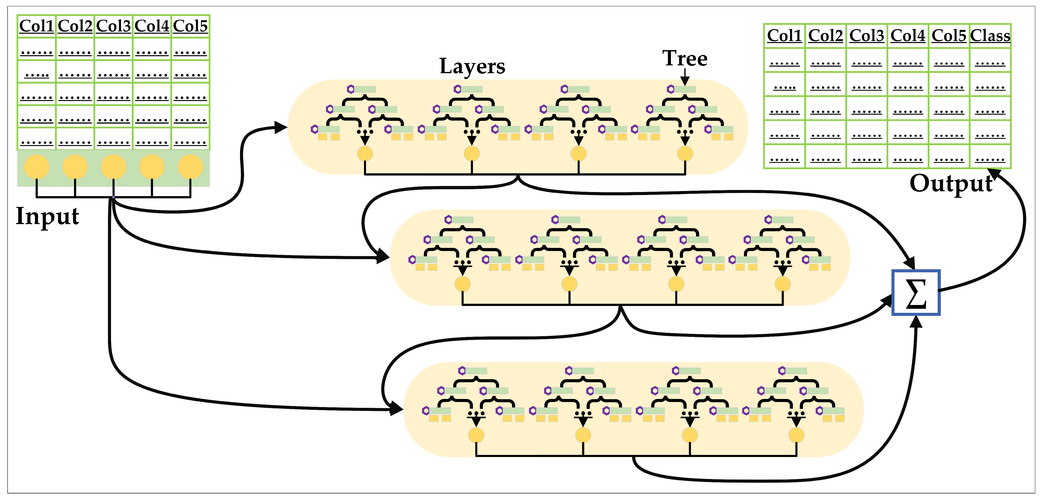
Many DL models for tabular data have also been introduced [35]. As depicted in Figure 2, those models take a completely different approach when compared with CNNs. For instance, the input for those models is a table (could be a table of features extracted for each segment), and the output is a class label for each row (each segment). Tabular DL models can be divided into differentiable trees and attention-based models [36]. The DT ensembles that exhibit robust performance with tabular data inspire differentiable tree models. DTs, however, do not support gradient optimization and are not differentiable. The smooth decision function and differentiable tree routine have been proposed in multiple studies [37,38]. Newer attention-based models [39,40,41] use inter- and intra-sample attention to account for the interaction between the properties of a particular sample and data points. Compared to shallow classifiers, outcomes from DL models are superior for tabular data [37,39,42]. Even though those tabular models align with the GEOBIA workflow, their effectiveness in extracting buildings using the GEOBIA framework has not yet been studied.

The major challenge of extracting buildings from high-resolution RGB images is retrieving spectral detail and improving the discrimination of buildings from other non-building objects. Although hundreds of features can be extracted for each segment based on their spectral, geometric, and textural properties, there is no clear indication of which RGB features are important for differentiating buildings from other objects. Classifiers used in the GEOBIA method take features that are a statistical summary of all pixels in a segment as input. However, as inter-segment homogeneity and intra-segment heterogeneity are usually high in high-resolution images, segment-level summaries exaggerate these characteristics and lead to misclassification [43] when using the shallow classifier. None of the previous studies have examined how well DL tabular models handle segment-level summaries when extracting features.

To address the challenges mentioned above and to evaluate the performance of different classifiers’ building extraction accuracy, this study utilized both SL and tabular DL classifiers simultaneously to examine their effectiveness in extracting buildings under the GEOBIA framework. The objective of this article was to conduct a detailed evaluation of the effectiveness of DL tabular models in the differentiation of buildings from diverse land covers. The article outlines the challenges faced by different classifiers during this differentiation process. Additionally, it emphasizes situations where SL classifiers demonstrated performance comparable to their DL counterparts. As a result, this study presents its findings separately to offer a thorough comprehension, opting not to amalgamate them into a final classification map.

First, the image was segmented using a hybrid segmentation method, and then spectral, textural, and geometrical features were extracted and stored in tabular format for each segment. Following the guideline of Ghanea et al. [2], buildings were identified from non-buildings such as shadows, vegetation, soil, and roads using different SL and tabular DL classifiers. The remaining sections of this paper are organized as follows: Section 2 presents the methodological framework, which includes image segmentation, feature extraction, classifiers, and accuracy assessment measures. Section 3 describes the study area and data used in this research. Section 4 presents the performance of the classifiers in distinguishing buildings from other non-building features, as well as heterogeneity within a roof. Section 5 offers a discussion based on the results obtained in the previous section. Finally, Section 6 presents the conclusions and future work.

2. Methodological Framework

2.1. Image Segmentation

Image segmentation in GEOBIA involves dividing an image into disjointed regions and grouping pixels into image objects. There are four main categories of image segmentation: pixel-based, edge-based, region-based, and hybrid [22]. Pixel-based methods involve thresholding and segmentation in the feature space, while edge-based segmentation involves identifying edges between regions and determining the segments within these edges. Region-based segmentation starts within an object and expands outward until it reaches its boundaries. Hybrid methods attempt to combine the strengths of edge- and region-based methods to improve results. This study employed a hybrid segmentation algorithm proposed by Hossain and Chen [16], which combines both edge-based and region-based methods. Initially, segments were generated using an edge-based approach, and subsequently merged using a region-based method. The watershed transformation was applied to the gradient image derived from RGB images to produce over-segmented initial segments. Following this, a region adjacency graph (RAG) was employed to delineate the adjacent relationships between segments.

To determine the suitability of merging, various metrics, including homogeneity, heterogeneity, illumination difference, rectangularity, and compactness between neighboring segments, were computed. Sample buildings were introduced to establish the threshold value for segment merging. Segments meeting the threshold and compactness criteria were merged, with the process iterated in loops. Each loop involved the utilization of reference buildings to ascertain the merging threshold. In cases where no segments met the merging criteria and a segment had only an encompassing neighbor, it was merged with said neighbor, disregarding the threshold. Unlike conventional segmentation algorithms, this approach utilized reference buildings to derive merging criteria, thus requiring minimal user input. Notably, the algorithm demonstrated the ability to segment buildings with minimal under-segmentation, despite the presence of over-segmentation, as depicted in Figure 3.

2.2. Object-Based Feature Extraction

The image segments were analyzed using object-based features considering spectral, geometric, and contextual characteristics. A previous study [27] found that spectral features are the most important in analyzing UAV images using the GEOBIA framework and that shape features should receive more attention. The GLCM (gray-level co-occurrence matrix) measures of homogeneity, angular second moment, and mean were found to be important in various scales. Another study [44] also utilized spectral, geometric, and textural features in their GEOCNN (geographic convolutional neural network) for object classification. This approach extracted the image objects’ spectral, geometric, and textural features according to these guidelines. The equation and its components for the selected object features are represented in

Table 1. Features extracted for GEOBIA classification.

Feature	Attribute	Mathematical Formulation
Spectral	Brightness [44]	$B=\frac{1}{n_{vis}}{\displaystyle \sum _{i=1}^{n_{vis}}}{\overline{b}}_{i\left(vis\right)}$ where B is an object’s average brightness, ${\overline{b}}_{i\left(vis\right)}$ is its average brightness in the visible bands, and $n_{vis}$ is its band count
	Mean band [44]	${\overline{C}}_k\left(v\right)={\overline{C}}_k\left(P_v\right)=\frac{1}{\#P_v}{\displaystyle {\displaystyle \sum }_{\left(x, y, z\right)ϵP_v}}{\overline{C}}_k\left(x, y, z\right)\left[C_k^{min}, C_k^{max}\right]$
	Standard deviation [44]	${\sigma }_k\left(v\right)={\sigma }_k\left(P_v\right)\sqrt{\frac{1}{\#P_v} \left({\displaystyle {\displaystyle \sum }_{\left(x, y, z\right)ϵP_v}}{C}_k^2\left(x,y,z\right)-\frac{1}{\#P_v}({\displaystyle {\displaystyle \sum }_{\left(x, y, z\right)ϵP_v}}{C}_k^2{\left(x,y,z\right)}^2)\right)}\left[0, \frac{1}{2}{C}_k^{range}\right]$ where ${\sigma }_k\left(v\right)$ represents the standard deviation of the intensity values for image layer k of all pixels that form an image object v; the set of pixels that belong to the image object v is denoted by $P_v$; the total number of pixels in $P_v$ is represented by $\#P_v$; the pixel coordinates are presented by $\left(x, y, z\right)$ and the image layer intensity value at each pixel is represented by $C_k\left(x, y, z\right)$; and $C_k^{range}$is the data range of image layer k, with $C_k^{range}$=$C_k^{max}-C_k^{min}$
	ExG [45]	$Ex{G}_v=2\ast {\overline{C}}_G\left(v\right)-{\overline{C}}_R\left(v\right)-{\overline{C}}_B\left(v\right)$ where $Ex{G}_v$ is the ExG value of a segment v, ${\overline{C}}_G\left(v\right)$ is the mean green band’s value for the segment v, ${\overline{C}}_R\left(v\right)$ is the mean red band’s value for the segment v, and ${\overline{C}}_B\left(v\right)$ is the mean blue band’s value for the segment v
	VIgreen [45]	$VIgree{n}_v=\frac{{\overline{C}}_G\left(v\right)}{{\overline{C}}_G{\left(v\right)}^a\ast {\overline{C}}_B{\left(v\right)}^{1-a}}$ where $VIgree{n}_v$ is the vegetation index of a segment v, ${\overline{C}}_G\left(v\right)$ is the mean green band’s value for the segment v, and ${\overline{C}}_B\left(v\right)$ is the mean blue band’s value for the segment v. a is a constant with a reference value of 0.667
	MGRVI [46]	$MGRV{I}_v=\frac{{\overline{C}}_G{\left(v\right)}^2-{\overline{C}}_R{\left(v\right)}^2}{{\overline{C}}_G{\left(v\right)}^2-{\overline{C}}_R{\left(v\right)}^2}$ where $MGRV{I}_v$ is the modified green–red vegetation indices of a segment v, ${\overline{C}}_G\left(v\right)$ is the mean green band’s value for the segment v, and ${\overline{C}}_R\left(v\right)$ is the mean red band’s value for the segment v.
	CIVE [45]	$CIV{E}_v=0.441 {\overline{C}}_R\left(v\right)-0.881 {\overline{C}}_G\left(v\right)+0.385 {\overline{C}}_B\left(v\right)+18.78745$ where $CIV{E}_v$ is the color index of vegetation of a segment v, ${\overline{C}}_R\left(v\right)$ is the mean red band’s value for the segment v, ${\overline{C}}_G\left(v\right)$ is the mean green band’s value for the segment v, and ${\overline{C}}_B\left(v\right)$ is the mean blue band’s value for the segment v.
	SAVI [45]	$SAV{I}_v=\frac{1.5\ast \left({\overline{C}}_G\left(v\right)-{\overline{C}}_R\left(v\right)\right)}{{\overline{C}}_G\left(v\right)+ {\overline{C}}_R\left(v\right)+0.5}$ where $SAV{I}_v$ is the soil adjusted vegetation index of a segment v, ${\overline{C}}_R\left(v\right)$ is the mean red band’s value for the segment v, and ${\overline{C}}_G\left(v\right)$ is the mean green band’s value for the segment v.
	ExGR [45]	$ExG{R}_v=Ex{G}_v-\left(1.4 {\overline{C}}_R\left(v\right)-{\overline{C}}_G\left(v\right)\right)$ where $ExG{R}_v$ is the excess green minus excess red index of a segment v, $Ex{G}_v$ is the excessive green for the segment v, ${\overline{C}}_R\left(v\right)$ is the mean red band’s value for the segment v, and ${\overline{C}}_G\left(v\right)$ is the mean green band’s value for the segment v.
	NGRDI [45]	$NGRD{I}_v=\frac{{\overline{C}}_G\left(v\right)-{\overline{C}}_R\left(v\right)}{{\overline{C}}_G\left(v\right)+ {\overline{C}}_R\left(v\right)}$ where $NGRD{I}_v$ is the normalized green–red difference index of a segment v, ${\overline{C}}_R\left(v\right)$ is the mean red band’s value for the segment v, and ${\overline{C}}_G\left(v\right)$ is the mean green band’s value for the segment v.
	NGBDI [46]	$NGBD{I}_v=\frac{{\overline{C}}_G\left(v\right)-{\overline{C}}_B\left(v\right)}{{\overline{C}}_G\left(v\right)+ {\overline{C}}_B\left(v\right)}$ where $NGBD{I}_v$ is the normalized green–blue difference index of a segment v, ${\overline{C}}_B\left(v\right)$ is the mean blue band’s value for the segment v, and ${\overline{C}}_G\left(v\right)$ is the mean green band’s value for the segment v.
	DSBI [47]	$DSB{I}_v=0.5\ast ({\overline{C}}_B\left(v\right)-{\overline{C}}_R\left(v\right))+0.5\ast ({\overline{C}}_B\left(v\right)-{\overline{C}}_G\left(v\right))$ where $DSB{I}_v$ is the difference spectral building index of a segment v, ${\overline{C}}_B\left(v\right)$ is the mean blue band’s value for the segment v, and ${\overline{C}}_G\left(v\right)$ is the mean green band’s value for the segment v.
Geometric	Length/width [44]	$\frac{length}{width}$ where $length$ denotes the length of the segment; $width$ represents the width of the segment
	Asymmetry [44]	$1-\frac{{\lambda }_{min}}{{\lambda }_{max}}$ where ${\lambda }_{min}$ is the minimal eigenvalue; ${\lambda }_{max}$ is the maximum eigenvalue
	Rectangularity [44]	$\frac{area}{minimum bounding rectange}$
	Shape index [44]	$\frac{B_v}{\sqrt[4]{\#V_v}}$ where $B_v$ is the segment’s border length; $\sqrt[4]{\#V_v}$ is the border of the square with the area of $\#P_v$
	SI [48]	$S{I}_v=\frac{P\left(v\right)}{4\ast \sqrt{A\left(v\right)}}$ where $S{I}_v$ is the shape index of a segment v, $P\left(v\right)$ is the perimeter, and $A\left(v\right)$ is the area of the segment v.
	Perimeter	Perimeter of a segment
Textural	Contrast [44]	${\displaystyle \sum }_{i,j=0}^{N-1}{P}_{i,j}{\left(i-j\right)}^2$ In the context of textural measures, the notation, $i$ represents the row number; $j$ represents the column number; $N$ is the total number of rows or columns; and $P_{i,j}$ denotes the probability value derived from the GLCM. It is important to note that these notations can also be applied to other textural measures described below.
	Correlation [44]	${\displaystyle \sum }_{i,j=0}^{N-1}{P}_{i,j}\left[\frac{\left(i-{\mu }_i\right)\left(j-{\mu }_i\right)}{\sqrt{\left({\sigma }_i^2\right)}\left({\sigma }_j^2\right)}\right]$ where σ is the GLCM standard deviation; ${\mu }_i$ is the GLCM mean
	Entropy [44]	${\displaystyle \sum }_{i,j=0}^{N-1}{P}_{i,j}\log P_{i,j}$
	Homogeneity [44]	${\displaystyle \sum }_{i,j=0}^{N-1}\frac{P_{i,j}}{1+\left|i-j\right|}$
	Angular second moment [44]	${\displaystyle \sum }_{i,j=0}^{N-1}{\left(P_{i,j}\right)}^2$
	Mean [44]	${\mu }_i={\displaystyle \sum }_{i,j=0}^{N-1}i\left(P_{i,j}\right), {\mu }_j={\displaystyle \sum }_{i,j=0}^{N-1}j\left(P_{i,j}\right)$
	Standard deviation [44]	${{\sigma }_i}^2=\sum _{i,j=0}^{N-1}{P}_{i,j}{\left(i-{\mu }_i\right)}^2, {{\sigma }_j}^2={\displaystyle \sum }_{i,j=0}^{N-1}{P}_{i,j}{\left(j-{\mu }_i\right)}^2$

. As in UAV images, there was no infrared band; this study calculated many indices available in the literature to differentiate buildings from other image objects. This study did not apply any feature reduction techniques; instead, it used all the features for object classification in GEOBIA. However, essential features for extracting differently colored buildings and other objects were identified using the variable/feature importance option in the classifiers.

2.3. SL Classifiers

Ensemble methods are a type of machine learning that combine several weak classifiers to create a single strong classifier. The DT classifier [49], widely used in GEOBIA, is a common weak learner often included in ensembles to improve classification performance. The RF [50] algorithm randomly selects a subset of features to use for classifying each DT and has the ability to detect mislabeled examples in the training data before predicting unlabeled samples. Two hyperparameters must be set to train an RF model: the number of features (Mtry) used for splitting at each node and the number of trees (Ntree) in the model. According to Ma et al. [23], reasonable accuracy can be achieved on various datasets when Mtry is set to log2(M) + 1, where M is the number of variables. In addition, Belgiu and Drǎguţ [51] used as large an Ntree value as possible, but Lawrence et al. [52] found that an Ntree of 500 or more provides unbiased error estimates. This study’s hyperparameters were fine-tuned using grid search and cross-validation on the training samples.

Boosting algorithms are a popular choice in remote sensing [32] as they involve training DTs sequentially, resulting in a lower error rate. AdaBoost (Adaptive Boosting) was developed to improve the accuracy of DTs [53]. This approach was later improved upon with the introduction of Gradient Boosting (GB), which fits an additive model to the gradient residual of the loss function. Another DT model used in remote sensing is the Classification and Regression Tree (CART), which divides the training dataset into subsets by applying a splitting rule to a single feature and uses the Gini Index and homogeneity criteria to maximize subset purity [54]. Extensive gradient boosting (XGB) is popular in the remote-sensing community [32,55,56]. Like RF, the XGB model identifies feature importance and divides the complex dataset into smaller subsets. The XGB method was also fine-tuned using grid search and cross-validation on the training samples.

An SVM is an SL classifier that has been shown to produce excellent results in classifying remote-sensing images [57]. SVM is a binary classifier that finds a linear hyperplane to separate two classes and aims to maximize the distance between the hyperplanes to reduce generalization error. Different kernel functions, such as the polynomial kernel, sigmoid kernel, radial basis function, and linear kernel, can be used in an SVM, and the choice of kernel function can significantly impact performance. SVMs also incorporate a penalty parameter to consider misclassification errors [54]. This classifier effectively handles continuous and categorical variables, as well as non-linear, complex, and noisy data with outliers, and helps prevent overfitting in the model. An SVM has two parameters that need to be tuned: C (the penalty parameter for the error term) and ε (the margin of tolerance). These parameters were selected using cross-validation and grid-search on the training samples.

2.4. DL Classifiers

The DL algorithm TabNet [39,58] was created for classification and regression tasks involving tabular data. The main principle of TabNet is to learn which elements of the input data to focus on at each level of the neural network by using attention processes. A subset of the input features is chosen for each decision step in the TabNet algorithm and is then processed by a neural network. Afterward, the results of various decision-making processes are pooled to provide a final prediction. In several tabular data classification and regression tasks, TabNet has been demonstrated to achieve state-of-the-art performance while also providing interpretable feature relevance scores. This algorithm offers several parameters, such as the size of the decision embedding space, the size of the attention embedding space, the number of decision steps, and the initial learning rate to tune up. TabNet’s capacity to learn interpretable feature importance ratings is one of its unique characteristics.

Combining feature tokenization with transformer-based models forms the foundation of the feature tokenizer + transformer (FTT) architecture [36]. By encoding categorical and numerical characteristics into a collection of fixed-length vectors, feature tokenization can be used to generate inputs for a transformer model. The transformer model’s deep learning architecture uses attention processes to discover connections between input features. It comprises numerous feedforward and self-attention neural network layers, allowing the model to recognize intricate correlations between variables and produce precise predictions [59]. FTT has several advantages over more conventional methods. It can process input features with large dimensions and non-linearity and automatically learn how features interact without the need for manual feature engineering. This makes it an effective tool for regression, classification, and predictive modeling projects.

A typical machine learning approach used for both tabular classification and regression issues is the Gated Additive Tree Ensemble (GATE) [42]. It is built on the idea of assembling many DTs, which are then joined using a gating mechanism to increase the model’s overall accuracy. The gating method enables the model to evaluate the contribution of each tree and make more informed decisions about the final forecast. Since the algorithm is additive, additional trees can be added to the ensemble at any time to enhance performance. This makes it adaptable and scalable to handling various data formats and application domains. The number of trees, tree depth, number of splits, learning rate, etc., are the main parameters to tune up in the GATE model. This algorithm has been shown to be highly effective in many real-world applications.

DTs and NNs are combined in a type of neural network architecture called a Neural Oblivious Decision Ensemble (NODE) [37]. They are appropriate for a variety of machine learning applications since they are made to offer both high accuracy and interpretability. The neural network in the NODE functions as an ensemble, combining the predictions of various DTs [36]. Each DT forms independent forecasts while unaware of the other trees. As a result, NODEs can handle both tabular and non-tabular data with ease and can grow to massive datasets. The interpretability of the NODE is one of its main benefits. The model’s decision-making process is simple because each DT operates independently [60]. The number of DTs, the depth of each tree, and the total number of neurons in the neural network are the primary hyperparameters for NODEs. The number of DTs determines the ensemble size, which can be set to a high value to improve model precision. Each tree’s depth can be changed to regulate the decision boundaries’ level of complexity and guard against overfitting.

2.5. Object Classification

This study employed the Python programming language to implement all classifiers. It also utilized PyTorch Tabular [35] to implement the deep learning classifiers. This research used an Nvidia Quadro P2000 GPU to develop the networks because PyTorch supports building deep learning networks on GPUs, significantly decreasing the execution time during training. An SVM and RF were implemented on scikit-learn, the most popular Python machine learning module. For the XGB classifier, the Python XGBoost module was used, and parameters were tuned using grid search and cross-tabulation on training data. Choosing a stopping criterion while training a neural network model is crucial since it helps prevent overfitting. This terminates the training process after a specific number of iterations. In this study, 500 iterations of training were used for all DL models. The Adam optimizer was used to minimize the loss function, and the learning rate was set at 0.001.

2.6. Accuracy Assessment

Precision (Equation (1)), recall/sensitivity (Equation (2)), overall accuracy (Equation (3)), and F1 score (Equation (4)) are commonly used evaluation matrices. They are defined as follows:

$$precision=\frac{TP}{TP+FP}$$

(1)

$$recall or sensitivity=\frac{TP}{TP+FN}$$

(2)

$$overall accuracy=\frac{TP+TN}{TP+TN+FP+FN}$$

(3)

$$F1=\frac{2\times precision\times recall}{precision+recall}$$

(4)

where TP, TN, FP, and FN indicate the number of true positives, true negatives, false positives, and false negatives, respectively. The number of segments accurately classified as buildings is referred to as TP, while TN denotes the number of segments correctly classified as non-buildings. On the other hand, the number of pixels that were incorrectly classified is represented by FP and FN. Precision is a measure that evaluates the ratio of the number of images accurately predicted as positive samples to all images predicted as positive samples. Recall, also known as sensitivity, calculates the proportion of positive samples that were correctly identified among all positive samples. The F1 score is a metric that takes into account both precision and recall. However, Silva et al. [61] stated that precision is not a reliable indicator of classification accuracy for building footprints because the non-building class has a more significant impact than the building class. They recommended specificity (Equation (5)) to determine true non-buildings that were correctly classified. Furthermore, they used the geometric mean (Equation (6)) to combine specificity and sensitivity measures, which helps to balance performance between positive and negative classes. This study also calculated both specificity and geometric mean measures.

$$specificity=\frac{TN}{TN+FP}$$

(5)

$$geometric mean=\sqrt{specificity x sensitivity}$$

(6)

3. Study Area and Data

For this research project, the city of Kingston, Ontario, Canada, was chosen as the study area (Figure 4). The training/validation utilized a UAV image with a spatial resolution of 0.20 m, consisting of three visible bands: red, green, and blue. As portrayed in Figure 4, this area contained various buildings of different sizes, shapes, and colors commonly found in urban areas. The study area included four types of roofs: gable (Figure 5a–c), hip (Figure 5d–f), complex (Figure 5g), and flat (Figure 5h), and there were some obstacles caused by nearby trees (Figure 5c,f) and building shadows (Figure 5b,e,g). Additionally, the footprint map was digitized by an image analyst, and a strict quality-control process was enforced to ensure that the digitized reference polygons were valid and accurate.

This study collected statistically independent and nonadjacent training and validating data (training/validating segments) using a list-frame approach to achieve unbiased analyses and outcomes. A total of 13,956 segments covering five distinct land-cover types—buildings (3645 samples), roads (2419 samples), soil (3148 samples), vegetation (2691 samples), and shadows (2053 samples)—were gathered for training the classifiers. The same samples were used in all classifiers for training. A total of 15,822 segments—buildings (3701 samples), roads (3000 samples), soil (3962 samples), vegetation (2659 samples), and shadows (2500 samples)—were used for the testing set.

4. Results

To accurately extract buildings from images, it is essential to distinguish and eliminate non-building objects that may result in errors of commission or omission. Commission errors happen when non-building features are mistakenly identified as buildings, whereas omission errors occur when buildings are not detected due to non-building features in the images. Thus, it is valuable to identify which non-building objects, such as shadows, vegetation, and soil, are difficult to differentiate from buildings.

4.1. Buildings versus Shadows

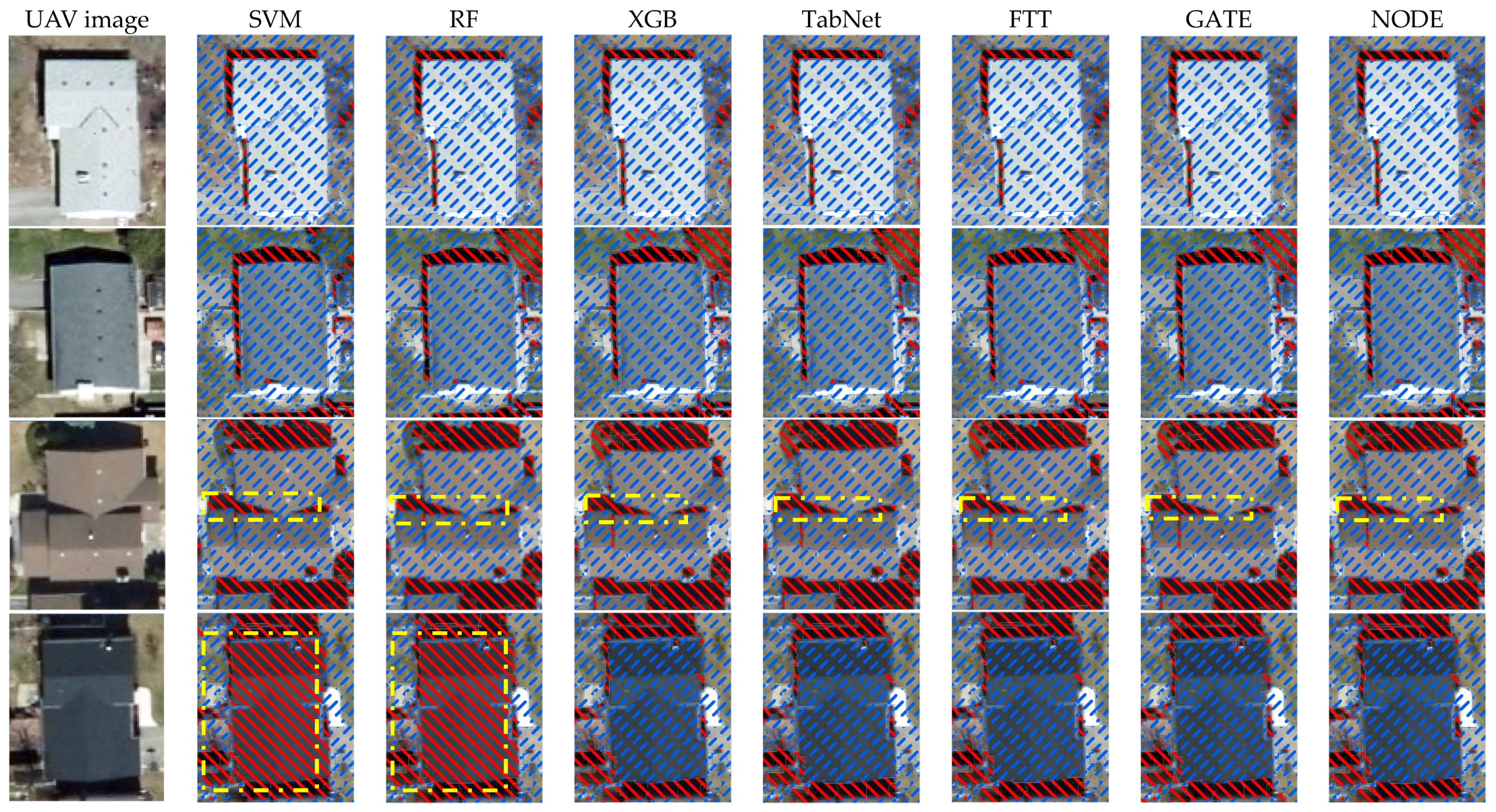
Initially, the classifiers were used to differentiate buildings from shadows. During the accuracy assessment, only two classes, namely shadows and building, were taken into account to determine which classifiers could better distinguish between the two and which features were essential to achieve this outcome. As shown in

Table 2. Accuracy measures for building vs. shadow classification for various classifiers.

Method	Precision/User Accuracy	Recall/Sensitivity/ Producer Accuracy	Overall	Specificity	Geometric Mean	F1
SVM	0.93	0.96	0.93	0.94	0.95	0.94
RF	0.96	0.98	0.97	0.97	0.97	0.97
XGB	0.97	0.99	0.98	0.98	0.98	0.98
TabNet	0.97	0.97	0.97	0.96	0.96	0.97
FTT	0.98	0.99	0.98	0.98	0.98	0.98
GATE	0.99	0.99	0.99	0.99	0.99	0.99
NODE	0.97	0.99	0.98	0.99	0.99	0.98

, GATE had the highest overall accuracy and F1 score. On the other hand, RF had lower precision and overall accuracy than other classifiers. As depicted in Figure 6, RF employed many features to achieve this result. In contrast, XGB relied heavily on the mean green band, mean RGB, and GLCM standard deviation and provided accuracy similar to other DL classifiers. Although the classifiers did an excellent job of segregating shadow from buildings, as illustrated in Figure 7 (in the dotted yellow box), except for GATE, all other classifiers classified a part or a full patch of the building as a shadow due to its spectral signature. Interestingly, as depicted in the third row of Figure 7, none of the classifiers could detect part of the building behind the shadow. In Figure 7, the red hatched area indicates the shadow, and the blue hatched area indicates non-shadow.

4.2. Buildings Versus Vegetation

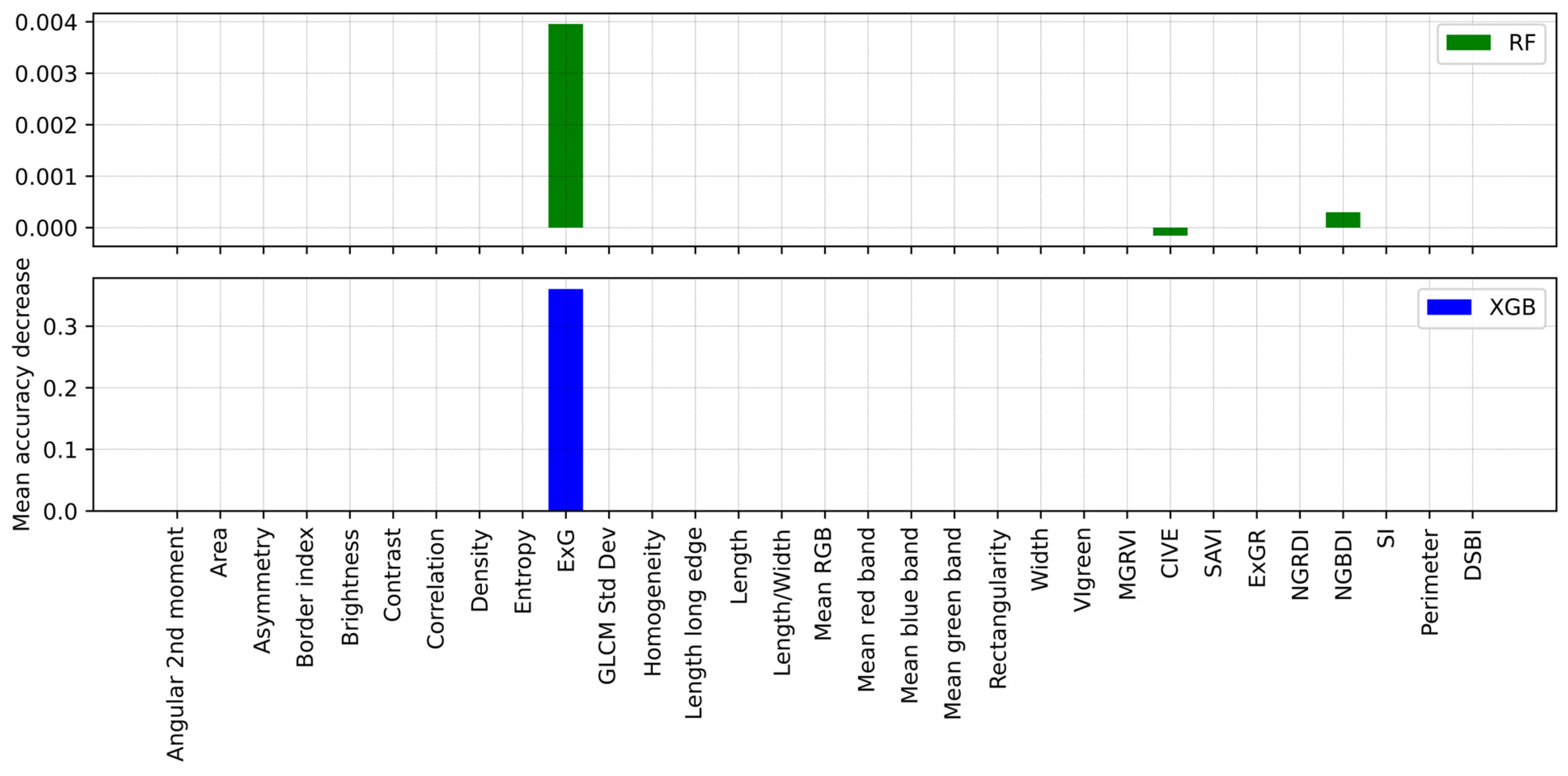
The UAV images used in this study were acquired in the spring. Thus, the lawns and backyards were still not fully green. The second step aimed to differentiate buildings from vegetation. During the accuracy assessment, only two classes, namely vegetation and buildings, were considered for determining which classifiers could better distinguish between the two and which features were crucial for achieving this objective. As shown in

Table 3. Accuracy measures for building vs. vegetation classification for various classifiers.

Method	Precision/User Accuracy	Recall/Sensitivity/ Producer Accuracy	Overall	Specificity	Geometric Mean	F1
SVM	0.97	0.99	0.98	0.99	0.99	0.98
RF	0.97	0.98	0.97	0.98	0.98	0.97
XGB	0.95	0.98	0.96	0.98	0.98	0.96
TabNet	0.91	0.98	0.93	0.97	0.97	0.94
FTT	0.98	0.99	0.98	0.99	0.99	0.98
GATE	0.97	0.99	0.98	0.98	0.98	0.98
NODE	0.99	0.99	0.99	0.98	0.98	0.99

, SVM and RF provided excellent results. On the other hand, TabNet had lower precision and overall accuracy compared to the other different classifiers. Interestingly, the shallow classifiers performed exceptionally well in this scenario. As depicted in Figure 8, XGB relied heavily on ExG to achieve this result. On the other hand, RF utilized ExG, NGBDI, and CIVE to classify objects. Although these classifiers successfully segregated vegetation from buildings, as shown in Figure 9 (in the dotted yellow box), RF, XGB, and TabNet classified part of the building as vegetation due to its spectral signature. In Figure 9, the green hatched area indicates vegetation, and the blue dashed area indicates non-vegetation.

4.3. Buildings versus Soil

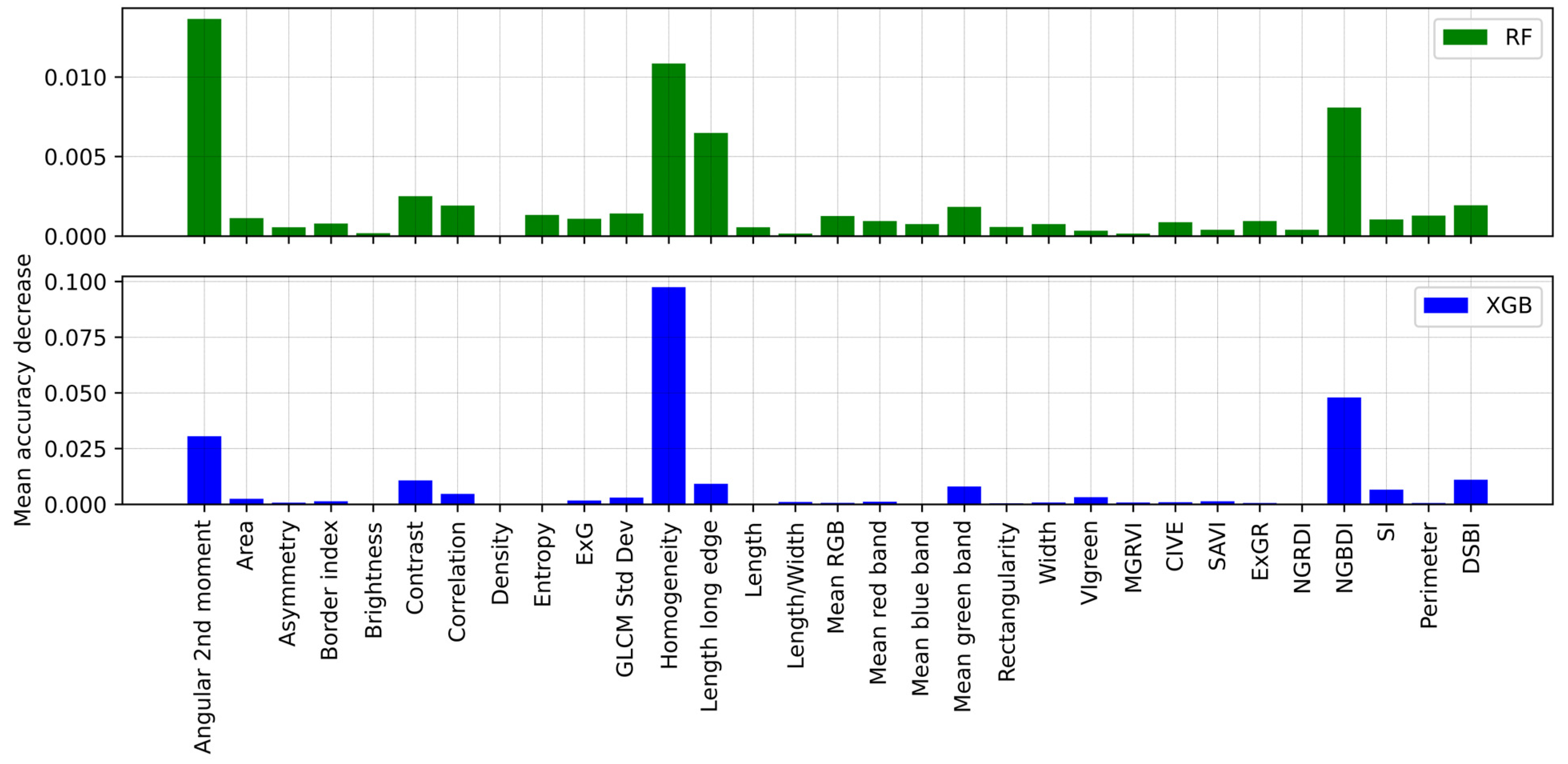
Due to the season, most of the deciduous shrubs in the study area had no leaves at all. The exposed branches and soil underneath made a unique spectral characteristic and covered a significant amount of the study area. After shadow and vegetation classification, the next target was to differentiate buildings from soil. During the accuracy assessment, only two classes, namely soil and buildings, were considered to determine which classifiers could better distinguish between the two and which features were crucial for achieving this objective. As shown in

Table 4. Accuracy measures for building vs. soil classification with various classifiers.

Method	Precision/User Accuracy	Recall/Sensitivity/ Producer Accuracy	Overall	Specificity	Geometric Mean	F1
SVM	0.99	0.97	0.99	0.97	0.97	0.98
RF	0.85	0.99	0.91	0.99	0.99	0.91
XGB	0.69	0.99	0.77	0.99	0.99	0.81
TabNet	0.57	0.99	0.63	0.96	0.97	0.72
FTT	0.92	0.99	0.95	0.99	0.99	0.95
GATE	0.99	0.99	0.99	0.99	0.99	0.99
NODE	0.78	0.99	0.86	0.99	0.99	0.87

, SVM and GATE had the highest overall accuracy and F1 score. On the other hand, TabNet had lower precision and overall accuracy compared to other classifiers. Interestingly, SVM performed exceptionally well in this scenario. As depicted in Figure 10, both RF and XGB relied heavily on homogeneity, angular second moment, and NGBDI to achieve this result. Although the classifiers successfully segregated the soil from the buildings, as shown in the dotted light green box in Figure 11, all classifiers classified part of the soil as non-soil due to its spectral signature. In Figure 11, the yellow hatched area indicates soil, and the blue hatched area indicates non-soil.

4.4. Buildings versus Other Impervious Surfaces

The next step was to examine the classifiers’ performance in segregating other impervious surfaces, such as roads, driveways, parking lots, etc., from the buildings. During the accuracy assessment, only two classes, namely other impervious surfaces and buildings, were considered to determine which classifiers could better distinguish between the two and which features were crucial for achieving this objective. As shown in

Table 5. Accuracy measures for building vs. other impervious surface classification by various classifiers.

Method	Precision/User Accuracy	Recall/Sensitivity/ Producer Accuracy	Overall	Specificity	Geometric Mean	F1
SVM	0.63	0.91	0.66	0.76	0.83	0.74
RF	0.55	0.95	0.54	0.37	0.59	0.70
XGB	0.54	0.96	0.54	0.26	0.50	0.69
TabNet	0.54	0.97	0.54	0.23	0.47	0.69
FTT	0.99	0.44	0.69	0.59	0.51	0.61
GATE	0.99	0.70	0.84	0.73	0.71	0.82
NODE	0.93	0.88	0.89	0.86	0.87	0.90

, all of the shallow and DL model classifiers performed poorly at this level. As depicted in Figure 12, both RF and XGB relied on the NGBDI, mean green band, DSBI, angular second moment, and ExG to achieve this result. NODE and GATE provided the highest overall accuracy and F1 score. As shown in the dotted yellow box in Figure 13, except NODE and GATE, RF, SVM, XGB, TabNet, and FTT either classified buildings as roads or roads as buildings due to their spectral signature. In Figure 13, the red hatched area indicates impervious surfaces, and the blue hatched area shows buildings and permeable surfaces.

4.5. Heterogeneity within a Building

Due to sun exposure, materials, and weather effects, individual building roofs displayed very different spectral properties and, thus, created two different segments for a building. In the next step, the flexibility of the classifiers to accommodate such variation was tested. This time, all of the non-building features were treated as a single class. This strategy was important as it provided a guideline for the post-classification analysis. As indicated in Figure 14, NGBDI, mean green band, angular second moment, ExG, correlation, and SI were used to classify segments. As shown in Figure 15, FTT classified part of the same building as a non-building. On the contrary, TabNet entirely missed that building and classified it all as a non-building.

5. Discussion

Automatic building extraction from remote-sensing images is important for urban planning, utility management, disaster management, resource allocation, and the production of topographic maps. Even though building extraction has received much attention over the years, it is still challenging as buildings show varied reflectance in spectral bands. Due to the complexity of building structures, the background in remote-sensing images, and similarity with other categories, building extraction results depend on the artificial feature design and adjustment. This can result in bias and poor generalization [62]. Researchers have recently proposed different pixel, length, edge, texture, semantic, and shadow-based building extraction methods. However, apart from the algorithms, their accuracy depends on the scale, image resolution, and image quality. Decimeter-level resolution achieved by UAV images enhances intra-class and reduces inter-class variance. Thus, manually designing classification features becomes challenging, and traditional recognition methods are unsuitable for building extraction.

Hossain and Chen [16] undertook a comparative analysis of building extraction methodologies, revealing that GEOBIA approaches yielded the least accuracy. Nevertheless, previous research efforts have failed to delve deeply into the factors contributing to this discrepancy, nor have they explored the potential impact of employing tabular DL classifiers. Notably, within GEOBIA methodologies, the manual extraction of features assumes a pivotal role. The literature abounds with the utilization of myriad features for object identification and classification. Previous studies have not thoroughly investigated the crucial features for distinguishing buildings from other objects, nor have they identified which non-building objects pose the greatest challenges for differentiation, especially for RGB images. In contrast, this research takes a comprehensive approach by extracting buildings based on their spectral signatures while also considering their differentiation from various land-cover types. To accomplish this, the study employed four DL models specifically designed for extracting buildings from images alongside three SL classifiers that have previously demonstrated satisfactory performance in GEOBIA research. Although the SL classifiers yielded acceptable results, their precision in identifying the buildings was not optimal. However, this study revealed that DL methods surpassed shallow classifiers in accurately identifying buildings, aligning with earlier research on tabular data classification. It is worth noting that not all DL models produced equivalent outcomes. GATE and NODE outperformed the others and consistently delivered superior results.

In the GEOBIA framework, the first and most important issue was image segmentation for extracting buildings. Although many algorithms are available for this purpose, none can produce perfect segments, meaning that a single image object, such as a building, is only placed under one segment [16]. Over-segmentation usually exists, and individual buildings are segmented into two or more segments, leading to a two-fold problem. First, each class requires more samples; secondly, individual buildings are classified as two different classes in some cases. As shown in the dotted yellow box in Figure 16, a part of the same roof was classified as two different land covers, whereas in Figure 17, due to under-segmentation, another land cover was merged with a roof and classified as a building. In this study area, residential buildings were dominant, and samples were mostly chosen from that category during image segmentation. As a result, commercial and educational buildings were over-segmented. Therefore, this study recommends different segmentation approaches for different land-cover types.

Individual segments can have numerous features extracted based on spectral, spatial, and textural properties. GEOBIA utilizes shallow classifiers, which perform differently across various studies and land-cover types. Unfortunately, most DL classifiers do not provide feature importance information. In this study, 31 features were extracted for each segment, and based on Table 2, Table 3 and Table 4, it was observed that RF and XGB utilized these features differently to identify different objects. Ma et al. [23] reported that feature reduction contributes differently to various classifiers. This study identified which features are essential in differentiating buildings from other land-cover types. Nevertheless, further analysis is required to examine and validate such results in different image settings. In the remote-sensing community, there is no consensus on which features provide the highest accuracy in most cases, nor is there a universal feature reduction technique.

In the literature, SL classifiers mostly used in GEOBIA performed poorly when extracting buildings from images, and different studies found contradictory results regarding their performance compared to each other. But the best part of these classifiers, especially RF and XGB, is that they provide feature importance, which guides future researchers when extracting features for classification. In addition, they require few parameter tunings. Even though the magnitude of feature importance varied between RF and XGB, this research observed a trend between them. Those classifiers performed well (like DL-based models) in differentiating buildings from shadows and vegetation. However, they failed to identify features such as soil and roads. Interestingly, those shallow classifiers performed even better than the DL TabNet model. This finding will guide future research in deciding whether or not they need to implement DL tabular models to differentiate buildings from shadow and vegetation.

Unlike SL classifiers, DL tabular models are still being developed, as all of the classifiers used in this study have been developed in the last few years. Not all DL models performed similarly in this study; for instance, TabNet performed poorly in most cases. Overall, TabNet performed poorly in all testing scenarios, while GATE and NODE performed better in all cases. However, they all struggled to differentiate roads and driveways from buildings. The spectral signatures and other features, such as rectangularity and different indices, are similar for all those land covers. This is the first study in which all of these DL models were used to identify buildings from RGB images. Shwartz-Ziv and Armon [60] pointed out that very few comparative studies have been conducted so far to identify the best classifiers. The reason behind this was the lack of standard benchmarks and the lack of open-source implementation for some models.

It is true that deep learning models typically have more complex architectures than shallow classifiers, necessitating more parameter adjustment during training. This is due to the fact that deep learning models have a large number of additional layers and parameters that must be optimized to obtain high accuracy. However, a GPU simplifies evaluating different parameter settings and can considerably speed up the training process. Transfer learning is an effective method for requiring less training data and optimizing weights with fewer iterations. It is possible to begin training a new model on a different dataset by using pre-trained models. This can speed up the process and increase accuracy. Previous studies, including the one by Novelli et al. [63], have demonstrated the effectiveness of using pre-trained models. As a result, this is a potential strategy for enhancing DL models’ accuracy in diverse applications. A hub or platform for model sharing could be established to facilitate the sharing of DL models in the remote-sensing community. This hub would allow researchers to easily access and utilize pre-trained models and share their models with others. Such a platform could help accelerate progress in the field of remote sensing and lead to better results.

6. Conclusions

Buildings are the most common locations and elements for human socio-economic activities. The characteristics of building types and their configuration in urban settlements can indicate the living population and implications for the placement of public services and the need for them. Due to their broad and frequent coverage, remote-sensing images have been widely used to detect urban land-use structures and buildings. Many building extraction methods have been developed for different remotely sensed data. The GEOBIA method has provided a better alternative to pixel-based methods for high-spatial-resolution images. However, building extraction from images using the GEOBIA framework is still a challenge. This study compared traditional shallow classifiers to recently proposed DL models and identified their effectiveness. Overall, the shallow classifiers performed poorly compared to the DL models. However, they provided similar performance in differentiating buildings from shadow and vegetation. Among the DL models, GATE and NODE offered superior performance. This is the first study where all of these classifiers were employed simultaneously to extract buildings from RGB images. Even though the DL models performed better than the shallow classifiers, they also could not differentiate buildings from other impervious surfaces in some cases.

The complexity of the image, insufficient cue extraction, and reliance on sensors are only a few of the difficulties that arise when automatically extracting buildings from image data [64]. It is difficult to identify buildings from other land covers in urban environments by using only spectral and textural features. Accurate building extraction must be achieved by combining spatial information with additional attributes to overcome these challenges. Various agencies are interested in the important information that differently colored roofs possess. Therefore, a practical strategy that may improve the classification accuracy of buildings based on their color is urgently needed. In order to compare different models, this study used crisp class labels provided by the classifiers and did not remove any object at each step. We are formulating a methodology for precisely extracting buildings based on the insights gained from this study. This involves employing deep learning tabular models, allowing for immediately classifying images for the entire area. This ongoing development reflects our commitment to enhancing the accuracy of and streamlining the remote-sensing process through advanced techniques.

References

1. Welch, R. Spatial Resolution Requirements for Urban Studies. Int. J. Remote Sens. 1982, 3, 139–146. [Google Scholar] [CrossRef]
2. Ghanea, M.; Moallem, P.; Momeni, M. Building Extraction from High-Resolution Satellite Images in Urban Areas: Recent Methods and Strategies against Significant Challenges. Int. J. Remote Sens. 2016, 37, 5234–5248. [Google Scholar] [CrossRef]
3. Ahmadi, S.; Zoej, M.J.V.; Ebadi, H.; Moghaddam, H.A.; Mohammadzadeh, A. Automatic Urban Building Boundary Extraction from High Resolution Aerial Images Using an Innovative Model of Active Contours. Int. J. Appl. Earth Obs. Geoinf. 2010, 12, 150–157. [Google Scholar] [CrossRef]
4. Hermosilla, T.; Ruiz, L.A.; Recio, J.A.; Estornell, J. Evaluation of Automatic Building Detection Approaches Combining High Resolution Images and LiDAR Data. Remote Sens. 2011, 3, 1188–1210. [Google Scholar] [CrossRef]
5. Chen, R.; Li, X.; Li, J. Object-Based Features for House Detection from RGB High-Resolution Images. Remote Sens. 2018, 10, 451. [Google Scholar] [CrossRef]
6. San, D.K.; Turker, M. Building Extraction from High Resolution Satellite Images Using Hough Transform. Int. Arch. Photogramm. Remote Sens. Spat. Inf. Sci. 2010, 38, 1063–1068. [Google Scholar] [CrossRef]
7. Lu, T.; Ming, D.; Lin, X.; Hong, Z.; Bai, X.; Fang, J. Detecting Building Edges from High Spatial Resolution Remote Sensing Imagery Using Richer Convolution Features Network. Remote Sens. 2018, 10, 1496. [Google Scholar] [CrossRef]
8. Yari, D.; Mokhtarzade, M.; Ebadi, H.; Ahmadi, S. Automatic Reconstruction of Regular Buildings Using a Shape-Based Balloon Snake Model. Photogramm. Rec. 2014, 29, 187–205. [Google Scholar] [CrossRef]
9. Huang, X.; Zhang, L. Morphological Building/Shadow Index for Building Extraction from High-Resolution Imagery over Urban Areas. IEEE J. Sel. Top. Appl. Earth Obs. Remote Sens. 2012, 5, 161–172. [Google Scholar] [CrossRef]
10. Benarchid, O.; Raissouni, N.; El Adib, S.; Abbous, A.; Azyat, A.; Achhab, N.B.; Lahraoua, M.; Chahboun, A. Building Extraction Using Object-Based Classification and Shadow Information in Very High Resolution Multispectral Images, a Case Study: Tetuan, Morocco. Can. J. Image Process. Comput. Vis. 2013, 4, 1–8. [Google Scholar]
11. Deng, X.; Li, W.; Liu, X.; Guo, Q.; Newsam, S. One-Class Remote Sensing Classification: One-Class vs. Binary Classifiers. Int. J. Remote Sens. 2018, 39, 1890–1910. [Google Scholar] [CrossRef]
12. Partovi, T.; Bahmanyar, R.; Kraus, T.; Reinartz, P. Building Outline Extraction Using a Heuristic Approach Based on Generalization of Line Segments. IEEE J. Sel. Top. Appl. Earth Obs. Remote Sens. 2017, 10, 933–947. [Google Scholar] [CrossRef]
13. Chai, D. A Probabilistic Framework for Building Extraction from Airborne Color Image and DSM. IEEE J. Sel. Top. Appl. Earth Obs. Remote Sens. 2017, 10, 948–959. [Google Scholar] [CrossRef]
14. You, Y.; Wang, S.; Ma, Y.; Chen, G.; Wang, B.; Shen, M.; Liu, W. Building Detection from VHR Remote Sensing Imagery Based on the Morphological Building Index. Remote Sens. 2018, 10, 1287. [Google Scholar] [CrossRef]
15. Gavankar, N.L.; Ghosh, S.K. Automatic Building Footprint Extraction from High-Resolution Satellite Image Using Mathematical Morphology. Eur. J. Remote Sens. 2018, 51, 182–193. [Google Scholar] [CrossRef]
16. Hossain, M.D.; Chen, D. A Hybrid Image Segmentation Method for Building Extraction from High-Resolution RGB Images. ISPRS J. Photogramm. Remote Sens. 2022, 192, 299–314. [Google Scholar] [CrossRef]
17. Kotaridis, I.; Lazaridou, M. Remote Sensing Image Segmentation Advances: A Meta-Analysis. ISPRS J. Photogramm. Remote Sens. 2021, 173, 309–322. [Google Scholar] [CrossRef]
18. Blaschke, T.; Hay, G.J.; Kelly, M.; Lang, S.; Hofmann, P.; Addink, E.; Feitosa, R.Q.; Van Der Meer, F.; Van Der Werff, H.; Van Coillie, F.; et al. Geographic Object-Based Image Analysis—Towards a New Paradigm. ISPRS J. Photogramm. Remote Sens. 2014, 87, 180–191. [Google Scholar] [CrossRef]
19. Ninsawat, S.; Hossain, M.D. Identifying Potential Area and Financial Prospects of Rooftop Solar Photovoltaics (PV). Sustainability 2016, 8, 1068. [Google Scholar] [CrossRef]
20. Som-ard, J.; Hossain, M.D.; Ninsawat, S.; Veerachitt, V. Pre-Harvest Sugarcane Yield Estimation Using UAV-Based RGB Images and Ground Observation. Sugar Tech. 2018, 20, 645–657. [Google Scholar] [CrossRef]
21. Liu, J.; Hossain, M.D.; Chen, D. A Procedure for Identifying Invasive Wild Parsnip Plants Based on Visible Bands from UAV Images. Int. Arch. Photogramm. Remote Sens. Spat. Inf. Sci. 2021, XLIII, 173–181. [Google Scholar] [CrossRef]
22. Hossain, M.D.; Chen, D. Segmentation for Object-Based Image Analysis (OBIA): A Review of Algorithms and Challenges from Remote Sensing Perspective. ISPRS J. Photogramm. Remote Sens. 2019, 150, 115–134. [Google Scholar] [CrossRef]
23. Ma, L.; Cheng, L.; Li, M.; Liu, Y.; Ma, X. Training Set Size, Scale, and Features in Geographic Object-Based Image Analysis of Very High Resolution Unmanned Aerial Vehicle Imagery. ISPRS J. Photogramm. Remote Sens. 2015, 102, 14–27. [Google Scholar] [CrossRef]
24. Zhang, C.; Sargent, I.; Pan, X.; Li, H.; Gardiner, A.; Hare, J.; Atkinson, P.M. An Object-Based Convolutional Neural Network (OCNN) for Urban Land Use Classification. Remote Sens. Environ. 2018, 216, 57–70. [Google Scholar] [CrossRef]
25. Hossain, M.D. An Improved Segmentation and Classification Method for Building Extraction from RGB Images Using GEOBIA Framework; Queen’s University: Kingston, ON, Canada, 2023. [Google Scholar]
26. Kucharczyk, M.; Hay, G.J.; Ghaffarian, S.; Hugenholtz, C.H. Geographic Object-Based Image Analysis: A Primer and Future Directions. Remote Sens. 2020, 12, 2012. [Google Scholar] [CrossRef]
27. Ma, L.; Li, M.; Ma, X.; Cheng, L.; Du, P.; Liu, Y. A Review of Supervised Object-Based Land-Cover Image Classification. ISPRS J. Photogramm. Remote Sens. 2017, 130, 277–293. [Google Scholar] [CrossRef]
28. Maxwell, A.E.; Strager, M.P.; Warner, T.A.; Ramezan, C.A.; Morgan, A.N.; Pauley, C.E. Large-Area, High Spatial Resolution Land Cover Mapping Using Random Forests, GEOBIA, and NAIP Orthophotography: Findings and Recommendations. Remote Sens. 2019, 11, 1409. [Google Scholar] [CrossRef]
29. Chawla, N.V.; Bowyer, K.W.; Hall, L.O.; Kegelmeyer, W.P. SMOTE: Synthetic Minority Over-Sampling Technique. J. Artif. Intell. Res. 2002, 16, 321–357. [Google Scholar] [CrossRef]
30. Douzas, G.; Bacao, F.; Fonseca, J.; Khudinyan, M. Imbalanced Learning in Land Cover Classification: Improving Minority Classes’ Prediction Accuracy Using the Geometric SMOTE Algorithm. Remote Sens. 2019, 11, 3040. [Google Scholar] [CrossRef]
31. Waldner, F.; Jacques, D.C.; Löw, F. The Impact of Training Class Proportions on Binary Cropland Classification. Remote Sens. Lett. 2017, 8, 1122–1131. [Google Scholar] [CrossRef]
32. Jozdani, S.E.; Johnson, B.A.; Chen, D. Comparing Deep Neural Networks, Ensemble Classifiers, and Support Vector Machine Algorithms for Object-Based Urban Land Use/Land Cover Classification. Remote Sens. 2019, 11, 1713. [Google Scholar] [CrossRef]
33. Maxwell, A.E.; Warner, T.A.; Fang, F. Implementation of Machine-Learning Classification in Remote Sensing: An Applied Review. Int. J. Remote Sens. 2018, 39, 2784–2817. [Google Scholar] [CrossRef]
34. Liu, B.; Du, S.; Du, S.; Zhang, X. Incorporating Deep Features into GEOBIA Paradigm for Remote Sensing Imagery Classification: A Patch-Based Approach. Remote Sens. 2020, 12, 3007. [Google Scholar] [CrossRef]
35. Joseph, M. PyTorch Tabular: A Framework for Deep Learning with Tabular Data. arXiv 2021, arXiv:2104.13638. [Google Scholar]
36. Gorishniy, Y.; Rubachev, I.; Khrulkov, V.; Babenko, A. Revisiting Deep Learning Models for Tabular Data. Adv. Neural Inf. Process. Syst. 2021, 23, 18932–18943. [Google Scholar]
37. Popov, S.; Babenko, A. Neural Oblivious Decision Ensembles for Deep Learning on Tabular Data. arXiv 2019, arXiv:1909.06312b. [Google Scholar]
38. Hazimeh, H.; Ponomareva, N.; Mol, P.; Tan, Z.; Mazumder, R. The Tree Ensemble Layer: Differentiability Meets Conditional Computation. In Proceedings of the 37th International Conference on Machine Learning, Online, 13–18 July 2020; pp. 4138–4148. [Google Scholar]
39. Arık, S.; Pfister, T. TabNet: Attentive Interpretable Tabular Learning. In Proceedings of the 35th AAAI Conference on Artificial Intelligence, Online, 2–9 February 2021; Association for the Advancement of Artificial Intelligence: Washington, DC, USA, 2021; Volume 35-8A, pp. 6679–6687. [Google Scholar]
40. Huang, X.; Khetan, A.; Cvitkovic, M.; Karnin, Z. TabTransformer: Tabular Data Modeling Using Contextual Embeddings. arXiv 2020, arXiv:2012.06678. [Google Scholar]
41. Somepalli, G.; Goldblum, M.; Goldstein, T. SAINT: Improved Neural Networks for Tabular Data via Row Attention and Contrastive Pre-Training. arXiv 2021, arXiv:2106.01342. [Google Scholar]
42. Joseph, M.; Raj, H. GATE: Gated Additive Tree Ensemble for Tabular Classification and Regression. In Proceedings of the 40th International Conference on Machine Learning, Honolulu, HI, USA, 23–29 July 2022. [Google Scholar]
43. Pan, X.; Zhang, C.; Xu, J.; Zhao, J. Simplified Object-Based Deep Neural Network for Very High Resolution Remote Sensing Image Classification. ISPRS J. Photogramm. Remote Sens. 2021, 181, 218–237. [Google Scholar] [CrossRef]
44. Feizizadeh, B.; Mohammadzade Alajujeh, K.; Lakes, T.; Blaschke, T.; Omarzadeh, D. A Comparison of the Integrated Fuzzy Object-Based Deep Learning Approach and Three Machine Learning Techniques for Land Use/Cover Change Monitoring and Environmental Impacts Assessment. GIScience Remote Sens. 2021, 58, 1543–1570. [Google Scholar] [CrossRef]
45. Beniaich, A.; Silva, M.L.N.; Avalos, F.A.P.; De Menezes, M.D.; Cândido, B.M. Determination of Vegetation Cover Index under Different Soil Management Systems of Cover Plants by Using an Unmanned Aerial Vehicle with an Onboard Digital Photographic Camera. Semin. Agrar. 2019, 40, 49–66. [Google Scholar] [CrossRef]
46. Yuan, Y.; Wang, X.; Shi, M.; Wang, P. Performance Comparison of RGB and Multispectral Vegetation Indices Based on Machine Learning for Estimating Hopea Hainanensis SPAD Values under Different Shade Conditions. Front. Plant Sci. 2022, 13, 928953. [Google Scholar] [CrossRef] [PubMed]
47. Gu, L.; Cao, Q.; Ren, R. Building Extraction Method Based on the Spectral Index for High-Resolution Remote Sensing Images over Urban Areas. J. Appl. Remote Sens. 2018, 12, 045501. [Google Scholar] [CrossRef]
48. Kurbatova, E. Road Detection Based on Color and Geometry Characteristics. In Proceedings of the 6th IEEE International Conference on Information Technology and Nanotechnology (ITNT), Samara, Russia, 26–29 May 2020; IEEE: Piscataway, NJ, USA, 2020; pp. 1–5. [Google Scholar]
49. Pal, M.; Mather, P.M. An Assessment of the Effectiveness of Decision Tree Methods for Land Cover Classification. Remote Sens. Environ. 2003, 86, 554–565. [Google Scholar] [CrossRef]
50. Breiman, L. Random Forests. Mach. Learn. 2001, 45, 5–32. [Google Scholar] [CrossRef]
51. Belgiu, M.; Drǎguţ, L. Random Forest in Remote Sensing: A Review of Applications and Future Directions. ISPRS J. Photogramm. Remote Sens. 2016, 114, 24–31. [Google Scholar] [CrossRef]
52. Lawrence, R.L.; Wood, S.D.; Sheley, R.L. Mapping Invasive Plants Using Hyperspectral Imagery and Breiman Cutler Classifications (RandomForest). Remote Sens. Environ. 2006, 100, 356–362. [Google Scholar] [CrossRef]
53. Chan, J.C.W.; Paelinckx, D. Evaluation of Random Forest and Adaboost Tree-Based Ensemble Classification and Spectral Band Selection for Ecotope Mapping Using Airborne Hyperspectral Imagery. Remote Sens. Environ. 2008, 112, 2999–3011. [Google Scholar] [CrossRef]
54. Mohajane, M.; Costache, R.; Karimi, F.; Bao Pham, Q.; Essahlaoui, A.; Nguyen, H.; Laneve, G.; Oudija, F. Application of Remote Sensing and Machine Learning Algorithms for Forest Fire Mapping in a Mediterranean Area. Ecol. Indic. 2021, 129, 107869. [Google Scholar] [CrossRef]
55. Georganos, S.; Grippa, T.; Vanhuysse, S.; Lennert, M.; Shimoni, M.; Wolff, E. Very High Resolution Object-Based Land Use-Land Cover Urban Classification Using Extreme Gradient Boosting. IEEE Geosci. Remote Sens. Lett. 2018, 15, 607–611. [Google Scholar] [CrossRef]
56. Bui, Q.T.; Chou, T.Y.; Van Hoang, T.; Fang, Y.M.; Mu, C.Y.; Huang, P.H.; Pham, V.D.; Nguyen, Q.H.; Anh, D.T.N.; Pham, V.M.; et al. Gradient Boosting Machine and Object-Based CNN for Land Cover Classification. Remote Sens. 2021, 13, 2709. [Google Scholar] [CrossRef]
57. Mountrakis, G.; Im, J.; Ogole, C. Support Vector Machines in Remote Sensing: A Review. ISPRS J. Photogramm. Remote Sens. 2011, 66, 247–259. [Google Scholar] [CrossRef]
58. Shah, C.; Du, Q.; Xu, Y.; Shah, C.; Du, Q.; Xu, Y. Enhanced TabNet: Attentive Interpretable Tabular Learning for Hyperspectral Image Classification. Remote Sens. 2022, 14, 716. [Google Scholar] [CrossRef]
59. Li, Q.; Wang, Y.; Shao, Y.; Li, L.; Hao, H. A Comparative Study on the Most Effective Machine Learning Model for Blast Loading Prediction: From GBDT to Transformer. Eng. Struct. 2023, 276, 115310. [Google Scholar] [CrossRef]
60. Shwartz-Ziv, R.; Armon, A. Tabular Data: Deep Learning Is Not All You Need. Inf. Fusion 2022, 81, 84–90. [Google Scholar] [CrossRef]
61. Silva, J.; Bacao, F.; Dieng, M.; Foody, G.M.; Caetano, M. Improving Specific Class Mapping from Remotely Sensed Data by Cost-Sensitive Learning. Int. J. Remote Sens. 2017, 38, 3294–3316. [Google Scholar] [CrossRef]
62. Wang, H.; Miao, F. Building Extraction from Remote Sensing Images Using Deep Residual U-Net. Eur. J. Remote Sens. 2022, 55, 71–85. [Google Scholar] [CrossRef]
63. Novelli, A.; Aguilar, M.A.; Aguilar, F.J.; Nemmaoui, A.; Tarantino, E. AssesSeg—A Command Line Tool to Quantify Image Segmentation Quality: A Test Carried Out in Southern Spain from Satellite Imagery. Remote Sens. 2017, 9, 40. [Google Scholar] [CrossRef]
64. Sohn, G.; Dowman, I. Data Fusion of High-Resolution Satellite Imagery and LiDAR Data for Automatic Building Extraction. ISPRS J. Photogramm. Remote Sens. 2007, 62, 43–63. [Google Scholar] [CrossRef]
Figure 1. Typical workflow of CNNs.
Remotesensing 16 00878 g001
Figure 2. A typical workflow of a DL-based tabular model.
Remotesensing 16 00878 g002
Figure 3. Segmentation results illustrated for a section of the study area with enhanced views for improved visualization.
Remotesensing 16 00878 g003
Figure 4. Location of the study area (Kingston ON, Canada) and the UAV test image.
Remotesensing 16 00878 g004
Figure 5. Sample types, shapes, and colors of the buildings available in the study area: gable roof (ac), hip roof (df), complex roof (g), and flat roof (h).
Remotesensing 16 00878 g005
Figure 6. Feature importance provided by RF (top) and XGB (bottom) for building versus shadow classification.
Remotesensing 16 00878 g006
Figure 7. Performance comparison of classifiers in differentiating buildings from shadows. The red hatched area indicates the shadow, the blue hatched area indicates non-shadow, and the yellow box indicates misclassification.
Remotesensing 16 00878 g007
Figure 8. Feature importance provided by RF (top) and XGB (bottom) for building versus vegetation classification.
Remotesensing 16 00878 g008
Figure 9. Performance comparison of classifiers in differentiating buildings from vegetation. The green hatched area indicates vegetation, the blue hatched area indicates non-vegetation, and the yellow box indicates misclassification.
Remotesensing 16 00878 g009
Figure 10. Feature importance provided by RF (top) and XGB (bottom) for building versus soil classification.
Remotesensing 16 00878 g010
Figure 11. Performance comparison of classifiers in differentiating buildings from soil. The yellow hatched area indicates soil, the blue hatched area indicates non-soil, and the light-green box indicates misclassification.
Remotesensing 16 00878 g011
Figure 12. Feature importance provided by RF (top) and XGB (bottom) for building versus other impervious surfaces classification.
Remotesensing 16 00878 g012
Figure 13. Performance comparison of classifiers in differentiating buildings from other impervious surfaces. The red hatched area indicates impervious surfaces, the blue hatched area indicates buildings and permeable surfaces, and the yellow box indicates misclassification.
Remotesensing 16 00878 g013
Figure 14. Feature importance provided by RF (top) and XGB (bottom) to extract heterogeneous roof type.
Remotesensing 16 00878 g014
Figure 15. Performance comparison of classifiers in extracting heterogeneous roof types. The purple hatched area indicates a non-building, and the blue hatched area shows a building.
Remotesensing 16 00878 g015
Figure 16. Over-segmentation-induced misclassification (as indicated in the yellow box). The green polygon designates a segment, the purple hatched area indicates a non-building, and the blue hatched area shows a building.
Remotesensing 16 00878 g016
Figure 17. Under-segmentation-induced misclassification (as indicated in the yellow box). The green polygon designates a segment, the purple hatched area indicates a non-building, and the blue hatched area shows a building.
Remotesensing 16 00878 g017