Spatial Resolution Enhancement of Vegetation Indexes via Fusion of Hyperspectral and Multispectral Satellite Data

Abstract

The definition and calculation of a spectral index suitable for characterizing vegetated landscapes depend on the number and widths of the bands of the imaging instrument. Here, we point out the advantages of performing the fusion of hyperspectral (HS) satellite data with the multispectral (MS) bands of Sentinel-2 to calculate such vegetation indexes as the normalized area over reflectance curve (NAOC) and the red-edge inflection point (REIP), which benefit from the availability of quasi-continuous pixel spectra. Unfortunately, MS data may be acquired from satellite platforms with very high spatial resolution; HS data may not. Despite their excellent spectral resolution, satellite imaging spectrometers currently resolve areas not greater than 30 × 30 m², where different thematic classes of landscape may be mixed together to form a unique pixel spectrum. A way to resolve mixed pixels is to perform the fusion of the HS dataset with the same dataset produced by an MS scanner that images the same scene with a finer spatial resolution. The HS dataset is sharpened from 30 m to 10 m by means of the Sentinel-2 bands that have all been previously brought to 10 m. To do so, the hyper-sharpening protocol, that is, $m:n$ fusion, is exploited in two nested steps: the first one to bring the 20 m bands of Sentinel-2 all to 10 m, the second one to sharpen all the 30 m HS bands to 10 m by using the Sentinel-2 bands previously hyper-sharpened to 10 m. Results are presented on an agricultural test site in The Netherlands imaged by Sentinel-2 and by the satellite imaging spectrometer recently launched as a part of the environmental mapping and analysis program (EnMAP). Firstly, the excellent match of statistical consistency of the fused HS data to the original MS and HS data is evaluated by means of analysis tools, existing and developed ad hoc for this specific case. Then, the spatial and radiometric accuracy of REIP and NAOC calculated from fused HS data are analyzed on the classes of pure and mixed pixels. On pure pixels, the values of REIP and NAOC calculated from fused data are consistent with those calculated from the original HS data. Conversely, mixed pixels are spectrally unmixed by the fusion process to resolve the 10 m scale of the MS data. How the proposed method can be used to check the temporal evolution of vegetation indexes when a unique HS image and many MS images are available is the object of a final discussion.

1. Introduction

The availability of hyperspectral (HS) and multispectral (MS) image data acquired by satellite platforms opened new horizons for the large-scale remote monitoring of vegetation, especially in impervious and uninhabited areas. Unfortunately, HS instruments produce a quasi-continuous spectrum, but with limited spatial resolution, typically 30 m pixel size, and on-demand acquisitions, so that it may become troublesome and expensive to perform constant monitoring over time. Conversely, MS scanners, like the Sentinel-2 twin constellation, feature global Earth coverage with a revisit time of five days at a spatial scale of up to 10 m. Unfortunately, they lack the spectral resolution that allows typical vegetation indexes to be accurately estimated. Sentinel-2 images, however, are easy to request and freely available for scientific purposes.

Here, we point out the advantages of performing the fusion of satellite HS data with the spectral bands of Sentinel-2 to calculate some vegetation indexes. Nevertheless, whereas chlorophyll indexes (CI), leaf area index (LAI), and normalized differential vegetation index (NDVI) were initially developed and validated using MS data, other indexes, such as the normalized area over reflectance curve (NAOC) and the red-edge inflection point (REIP), are more accurately estimated from HS data rather than MS data [1,2,3]. Definitions and implementations of such indexes depend on the number and bandwidths of the instrument. Especially, indexes that measure a property of reflectance spectra, like NAOC and REIP, become more and more accurate as the number of available bands increases. This issue motivates the spatial resolution enhancement of HS data, which is equivalent to the spectral resolution enhancement of MS data, which already possess an adequate spatial resolution.

Data fusion aimed at resolution enhancement is the joint processing of two datasets, with at least one being multiband, in order to synthesize an image product that ideally exhibits the spectral characteristics of the lower-spatial-resolution multiband image at the spatial resolution of the higher-resolution dataset [4]. When the higher-resolution dataset is a panchromatic (Pan) image, the spatial enhancement process is referred to as pansharpening [5]. If a Pan image is unavailable, or equivalently, the sharpening band is not unique, hyper-sharpening denotes the sharpening of the less spatially resolved set of bands by means of suitable combinations of the more spatially resolved bands, usually covering the visible and near infrared (VNIR) spectrum [6]. The goal is maximizing a matching function between the combination of the sharpening bands, which represents the synthesized Pan, and the lower-resolution band that shall be sharpened. The rationale lies in finding common spatial/spectral patterns between the sharpening and sharpened data, as originally devised for hyperspectral data compression [7]. Alternatively, hyper-sharpening may be brought back to blind source separation concepts [8]. Originally devised for single-platform data [6,9], hyper-sharpening has been extended to multi-platform data [10,11]. Since hyper-sharpening can be regarded as an MS-to-HS fusion, it can be tackled as problem of spectral unmixing, for which an approach based on spectral profiles has been recently proposed [12]. The HS dataset may be sharpened from 30 m to 10 m by means of the Sentinel-2 bands that have all been previously brought to 10 m. The hyper-sharpening protocol, i.e., m:n fusion, while pansharpening is 1:n fusion, has been exploited in two nested steps: one to bring all the 20 m bands of Sentinel-2 to 10 m and another to sharpen all the 30 m HS bands to 10 m by using the Sentinel-2 bands hyper-sharpened at 10 m. The spatial accuracy of vegetation indexes calculated from fused data is analyzed. Their temporal evolution is discussed, if a unique HS image and many MS images are available.

So far, few authors have investigated the effects of pansharpening on vegetation indexes [13], but nobody has ever analyzed the spatial upgrade of spectral information originated by hyper-sharpening, in which in principle there are as many different sharpening bands as there are bands to sharpen and thus, the sharpening dataset conveys the spectral information of the MS dataset. In fact, depending on the sharpening protocol, normalized spectral indexes, e.g., NDVI, obtained from sharpened data may be spatially enhanced or not. If the sharpening band is unique, as happens with pansharpening, it can be proven that there is no increase in spectral information at the finer spatial scale [14].

The remainder of this paper is organized as follows. Section 2 illustrates the HS and MS satellite data used in this study, reviews the hyper-sharpening protocol, presents the proposed approach for the fusion multi-platform data based on nested hyper-sharpening stages, introduces the statistical quality assessment of fusion with two new indexes devised ad hoc for hyper-sharpening, and reviews two indexes suitable for analyses of vegetated areas and their implementations from both HS and MS data. Section 3 presents the results of nested hyper-sharpening of EnMAP and Sentinel-2 data and discusses full-scale quality assessment. Later, an analysis of the estimation accuracy of vegetation indexes attainable by the original and fused HS and MS datasets is performed. Section 4 discusses the possible application of the proposed fusion procedure to the case of spatio-temporal fusion for the temporal monitoring of vegetated areas. Concluding remarks are drawn in Section 5.

2. Materials and Methods

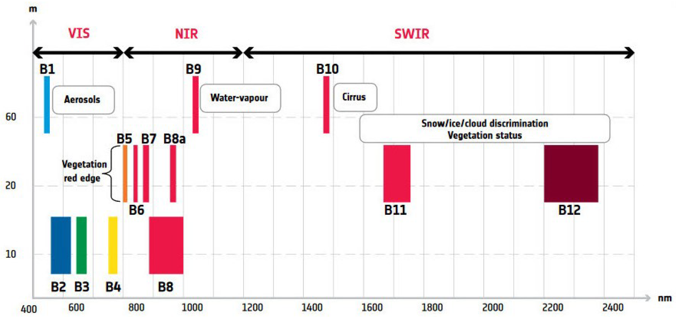
2.1. Hyperspectral and Multispectral Scanners from Space

The availability of HS datasets collected from space dates back to almost a quarter of century ago, with the pioneering push-broom Hyperion spectrometer on the Earth Observation-1 (EO-1) satellite, launched by NASA. EO-1 was also equipped with a 10-band MS scanner, including a 10 m Pan image [15]. Unfortunately, Hyperion featured a narrow swath (7.7 km) because of technological limitations and experienced serious miscalibration problems just a few years after its launch, a problem that new-generation spaceborne imaging spectrometers have brilliantly solved through an onboard calibration system based on fixed stars.

Twenty years after, technological advances led to the launch of two European HS missions: the Italian Space Agency’s PRISMA (Italian acronym for Hyperspectral Precursor of the Application Mission) [16] and the Environmental Mapping and Analysis Program (EnMAP) [17], managed by DLR German Agency. The main characteristics of the two missions and data products are the following. PRISMA was launched on 22 March 2019 and is equipped with: a HS sensor with a spatial sampling of 30 m × 30 m and a spectral sampling of 10 nm ranging from 400 nm to 2500 nm; a Pan camera with a bandwidth of 450–700 nm and a spatial sampling of 5 m × 5 m. EnMAP was launched on 1 April 2022 and is equipped with an imaging spectrometer capable of resolving 224 spectral bands from 420 to 2450 nm with a spectral sampling of 6.5 nm and 10 nm in the VNIR and short-wave infrared (SWIR) spectra, respectively, and a ground sampling of 30 m × 30 m.

In parallel, the Sentinel-2 twin satellite constellation (2A and 2B) of the European Space Agency (ESA) provides MS data in the VNIR and SWIR wavelengths at decametric spatial resolution, with global coverage of the Earth in five days. Among the Sentinel-2 bands, whose layout is shown in Figure 1, B5, B6, and B7 in the red-edge (RE) region, B11 and B12 in the SWIR region, and B8a, a narrow-band NIR centered at 865 nm, are provided at 20 m spatial sampling interval (SSI). Four other VNIR bands, namely, B2, B3, B4, and B8, are geocoded at 10 m SSI. The three 60 m bands, B1, B9, and B10, are less relevant for EO and are used for studies of the atmosphere to infer the content of aerosols, water vapor, and ice, respectively. The Sentinel-2 bands in the RE regions, namely, B5 and B6, with a 15 nm spectral width, and B7, with a 20 nm width, are provided at 20 m spatial resolution. Hyper-sharpening may improve the spatial resolution of the Sentinel-2 bands acquired at 20 and 60 m and the related spectral indexes, specifically those computed from the RE bands, suitable for studies on vegetation [18].

The EnMAP dataset used in this study was acquired on 10 August 2022 over an agricultural site north of Groningen, The Netherlands (NL). The data have been atmospherically corrected and geocoded through bilinear interpolation and UTM/WGS84 projection. The data format is normalized remote sensing reflectance (Rrs) on 224 spectral bands. After discarding eleven water vapor absorption bands in the SWIR wavelengths, the EnMAP data cube is formed by 213 bands. The Sentinel-2 dataset was acquired by the Sentinel-2B twin satellite on 10 August 2022 over the site of Groningen (NL). The data product is a Level-2A (atmospherically corrected surface reflectance images) UTM/WGS84 projection. Due to a satellite acquisition angle of zero degrees for Sentinel-2 and 11 degrees for EnMAP, there is a difference in the acquisition times of the two images of about one hour, while the acquisition day is the same.

2.2. A Review of Hyper-Sharpening

Whenever the sharpening image is not unique, hyper-sharpening deals with the synthesis of a unique sharpening image, the source of spatial details, to obtain the best-fused products [6]. This synthetic Pan may be different for each band.

Let ${\left\{{\mathbf{M}}_k\right\}}_{k=1,\dots ,N}$ denote the higher-resolution bands, e.g., the four 10 m VNIR bands of Sentinel-2; ${\left\{{\mathbf{H}}_i\right\}}_{i=1,\dots ,M}$ the lower-resolution bands, e.g., the three RE, the narrowband NIR and the two SWIR bands of Sentinel-2, all at 20 m spatial scale; and R the ratio between the spatial scales of $\mathbf{H}$ and $\mathbf{M}$ ($N=4$, $M=6$, and $R=2$ for Sentinel-2). The enhancing band ${\mathbf{P}}_i^{*},i=1,\dots ,M$ of the ith lower-resolution band, ${\mathbf{H}}_i$, is synthesized according to the following procedure.

First, the ${\mathbf{M}}_k$ bands are lowpass-filtered with a normalized cutoff frequency $1/R$, providing the bands ${\mathbf{M}}_{kL}$ degraded at the resolution of the bands that are being sharpened. Then, the relationship between the lower-resolution bands interpolated by a factor R, ${\tilde{\mathbf{H}}}_i$, and ${\mathbf{M}}_{kL}$ is modeled through a multivariate linear regression:

$${\tilde{\mathbf{H}}}_i={\widehat{w}}_0^{\left(i\right)}+\sum _{k=1}^N{\widehat{w}}_k^{\left(i\right)}·{\mathbf{M}}_{kL}+{ϵ}_{i}i=1,\dots ,M$$

(1)

in which ${ϵ}_i$ is the space-varying residue. The set of space-constant optimal weights, ${\left\{{\widehat{w}}_k^{\left(i\right)}\right\}}_{k=0,\dots ,N}$, is calculated as the minimum MSE (MMSE) solution of Equation (1). The weights, ${\widehat{w}}_k^{\left(i\right)}$, are used to synthesize the set of enhancing bands, ${\left\{{\mathbf{P}}_i^{*}\right\}}_{i=1,\dots ,M}$:

$${\mathbf{P}}_i^{*}={\widehat{w}}_0^{\left(i\right)}+\sum _{k=1}^N{\widehat{w}}_k^{\left(i\right)}·{\mathbf{M}}_{k}i=1,\dots ,M.$$

(2)

Finally, the sharpened bands, ${\widehat{\mathbf{H}}}_i$, at a 10 m resolution for Sentinel-2, are computed by applying a contrast-based fusion algorithm to ${\tilde{\mathbf{H}}}_i$ and ${\mathbf{P}}_i^{*}$:

$${\widehat{\mathbf{H}}}_i={\tilde{\mathbf{H}}}_i·\frac{{\mathbf{P}}_i^{*}}{{\mathbf{P}}_{iL}^{*}},i=1,\dots ,M.$$

(3)

in which ${\mathbf{P}}_{iL}^{*}$ is the lowpass-filtered version of ${\mathbf{P}}_i^{*}$, or, equivalently,

$${\mathbf{P}}_{iL}^{*}={\widehat{w}}_0^{\left(i\right)}+\sum _{k=1}^N{\widehat{w}}_k^{\left(i\right)}·{\mathbf{M}}_{kL}i=1,\dots ,M.$$

(4)

The three 60 m bands of Sentinel-2 may be either sharpened starting from the six 20 m bands, before the 20 m to 10 m sharpening step described in Equations (1)–(4) is performed, or directly sharpened from the set of 10 m bands, four original and six hyper-sharpened. In the former cases, the procedure consists of two nested hyper-sharpening steps: 60 m to 20 m followed by 20 m to 10 m. In the latter case, the nested steps are 20 m to 10 m followed by 60 m to 10 m.

Note that, for Sentinel-2, the sharpening bands and the sharpened bands are simultaneously acquired from the same platform. Conversely, for very/extremely high-resolution (VHR/EHR) MS scanners, e.g., WorldView-3, in which four instruments with three different resolutions are present [9], such an acquisition is not simultaneous but is made from different positions along the orbit. This fact may lead to local shifts between the two datasets [19] in the presence of hilly or mountainous terrain. The absence of misregistration entails the use of fusion methods based on multiresolution analysis, achieved through lowpass filters [20].

The coefficients of determination of the multivariate regressions in Equation (1),

$$R_i^2\triangleq 1-\frac{{\sigma }_{{ϵ}_i}^2}{{\sigma }_{{\tilde{\mathbf{H}}}_i}^2},$$

(5)

in which ${\sigma }_{{ϵ}_i}^2$ and ${\sigma }_{{\tilde{\mathbf{H}}}_i}^2$ denote the variance of the LS residue and of the interpolated low-resolution band, respectively, determine the histogram matching between each of the low-resolution bands and the enhanced image synthesized from the 10 m VNIR bands [5]. The use of a multivariate linear regression to synthesize the sharpening bands makes the method independent of the data format [21]. However, while the math derivation of the sharpening bands does not depend on the physical format of the data, e.g., spectral radiance or surface reflectance, the fusion rule in Equation (3), derived from the radiative transfer model [22], assumes that the data are expressed as surface reflectances.

While the spectral radiance is a level-one (L1) product, the surface reflectance is a level-two (L2) product and is usually distributed for global-coverage systems, like the two Operational Land Imager (OLI) instruments mounted on LandSat 8 and 9, and Sentinel-2A/B, where an instrument network exists for atmospheric measurements [23], which are performed through LiDARs [24], measuring the interaction with the atmosphere of laser beams [25]. If only the spectral radiance format is available, the data should be haze-corrected: each diminished by its atmospheric path radiance, or haze, when it is used in Equation (3). The estimation of the atmospheric path-radiance terms may follow image-based approaches [26] or rely on radiative transfer models of atmosphere and its constituents [27]. The haze term is zero for data in surface-reflectance format, whenever they are available. For the EnMAP dataset, the L2 surface reflectance product was available.

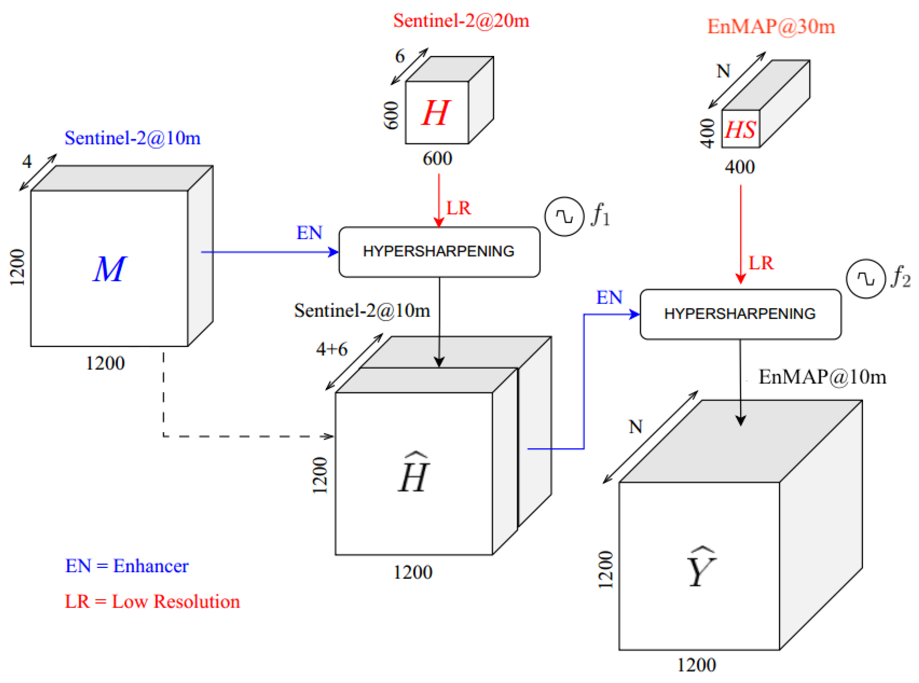
2.3. Flowchart of the Proposed Method

The proposed sharpening method is composed of two steps, graphically described in Figure 2. The number of steps is equal to the overall number of different resolutions concerned minus one: 30 m (EnMAP HS), 20 m (medium-resolution Sentinel-2 bands) and 10 m (high-resolution Sentinel-2 bands). The three 60 m bands of Sentinel-2 have been intentionally discarded because their resolution is lower than that of the HS datasets.

The inner stage concerns Sentinel-2 data only. The attention is focused on the three RE bands, whose relevance to the analysis of vegetation characteristics has been largely recognized [2], on the narrow NIR band B8a, and on the two SWIR broad bands. Originally produced at 20 m resolution, all these bands are hyper-sharpened by means of the four 10 m VNIR bands (see Figure 1).

• The six Sentinel-2 bands at 20 m resolution are hyper-sharpened to 10 m by means of a combination of the four 10 m VNIR bands, following Equations (1)–(4).
• The N 30 m HS bands, EnMAP in the present case, are hyper-sharpened at 10 m by means of a combination of the 10 m Sentinel-2 bands, four original and six hyper-sharpened, as described in Step 1. Each 30 m HS band is spatially enhanced at 10 m according to the hyper-sharpening protocol in Equations (1)–(4).

Note the presence of two nested hyper-sharpening boxes: the hyper-sharpening of HS data is achieved by means of MS data that have been previously hyper-sharpened.

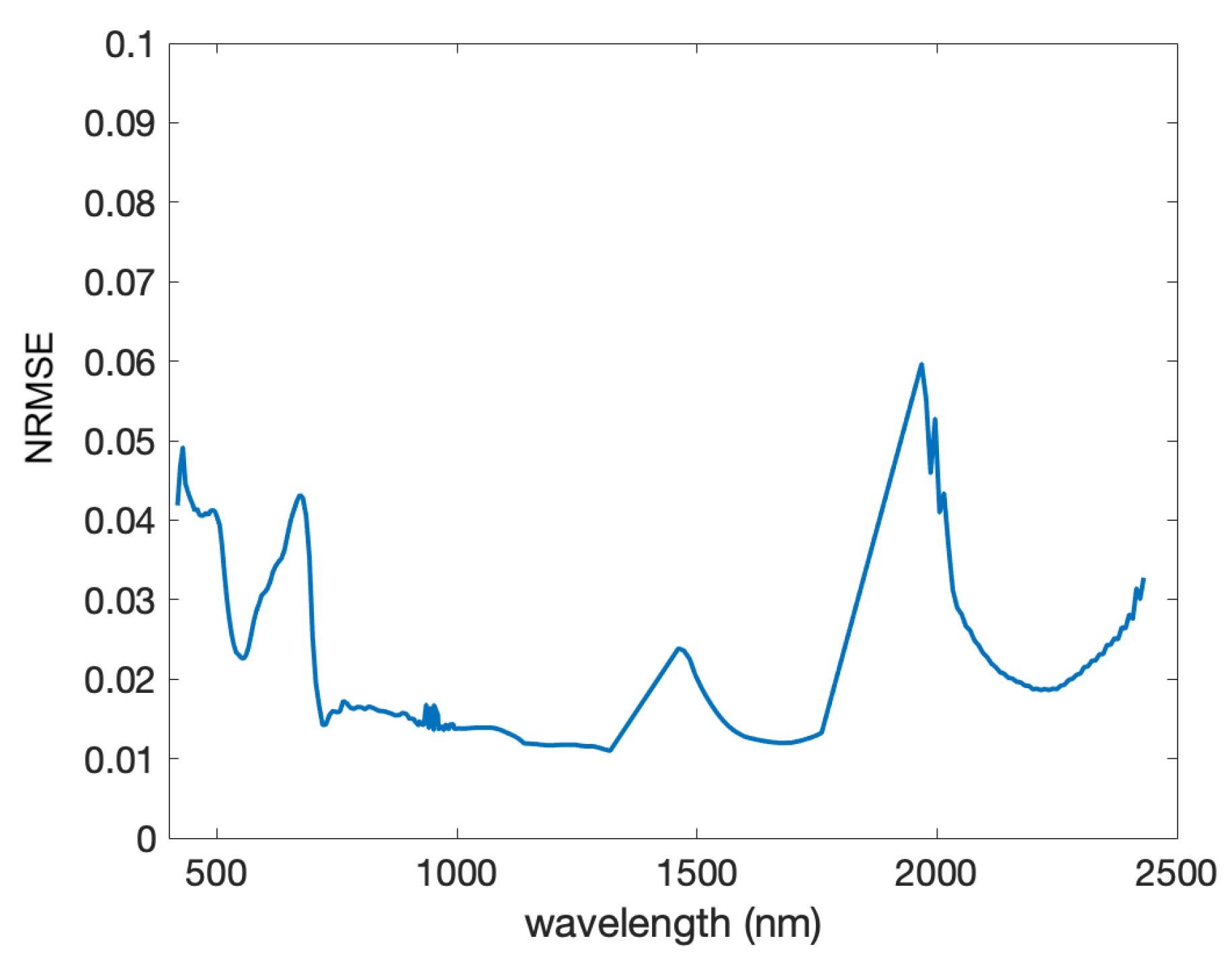
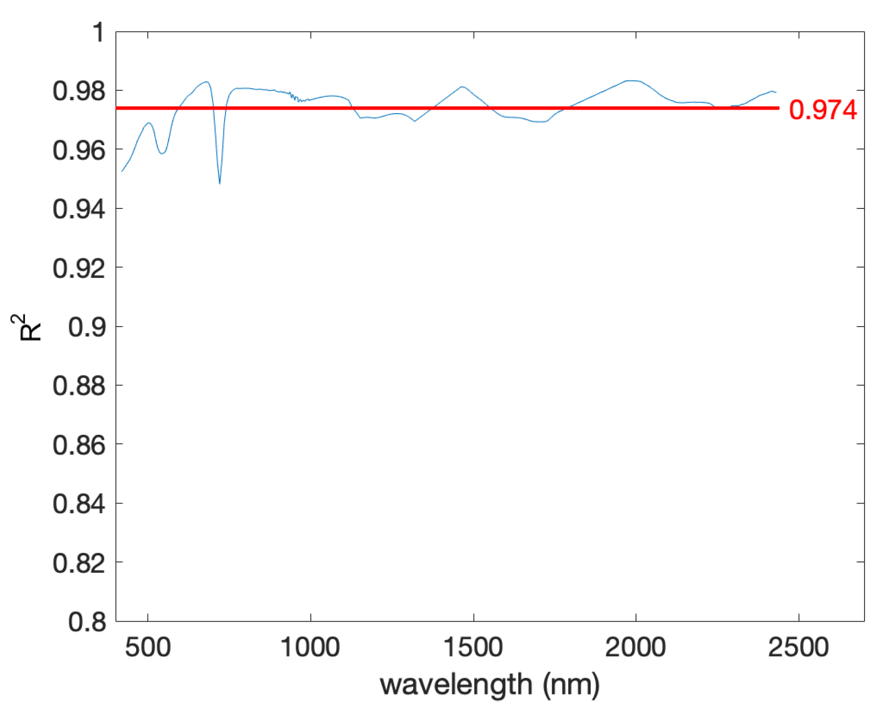
2.4. Statistical Quality Assessment of the Fused Dataset

Even though many efforts have been made since the problem was originally stated [28], quality assessments of fusion products remains an open problem [29,30]. Objective evaluations at full scale have been carried out in terms of separate measurements of spectral consistency of the fused HS data to the original HS data [31]. The spectral distortion of the quality with no reference (QNR) protocol [31], namely, $D_{\lambda }$, and the spatial distortion, $D_s^{*}$, based on the the multivariate regression of the sharpened bands to the Pan image [31,32] have been coupled together to yield a unique quality index, QNR*, normalized in [0, 1]:

$${\mathrm{QNR}}^{*}=(1-D_{\lambda })(1-D_s^{*})$$

(6)

in which the spatial consistency factor, $1-D_s^{*}$, reflects the ability of the sharpened bands to synthesize back the sharpening band and is defined as the coefficient of determination, $R^2$, of the MMSE solution of the multivariate regression of ${\widehat{\mathbf{H}}}_i$ towards either $\mathbf{P}$ or ${\mathbf{P}}_i^{*}$, defined in Equation (2), for pansharpening or hyper-sharpening, respectively. Thus, the definition of the spatial consistency, $1-D_s^{*}$, entails its extension to hyper-sharpening, for which the sharpening image is not unique.

Three statistical indexes, two of which have been specifically designed for the task of hyper-sharpening, have been used. The first index is known in the literature [6] and is the normalized root mean square error (NRMSE) between the original HS band and sharpened HS band after the spatial detail has been removed by means of a Gaussian lowpass filter, with a cutoff at one-third of the Nyquist frequency for a 3:1 scale ratio. NRMSE is normalized to the mean of the original HS band and plotted versus the wavelength.

The second index is a generalization of $1-D_s^{*}$ [19], originally defined for a unique Pan image, to the case of multiple (synthetic) Pan images. The index is calculated for the synthetic Pan of each HS band, defined in Equation (2), and plotted versus the wavelength. The index reflects the fraction of the spatial information of Sentinel-2 that is incorporated in each of the fused HS bands.

Eventually, if ${\mathbf{P}}_i^{*}$ is replaced with ${\mathbf{M}}_i^{*}$ in the multivariate regression, an inter-sensor consistency index can be defined as the ability of the sharpened bands of the lower-spatial-resolution instrument to synthesize each of the bands of the higher-resolution instrument.

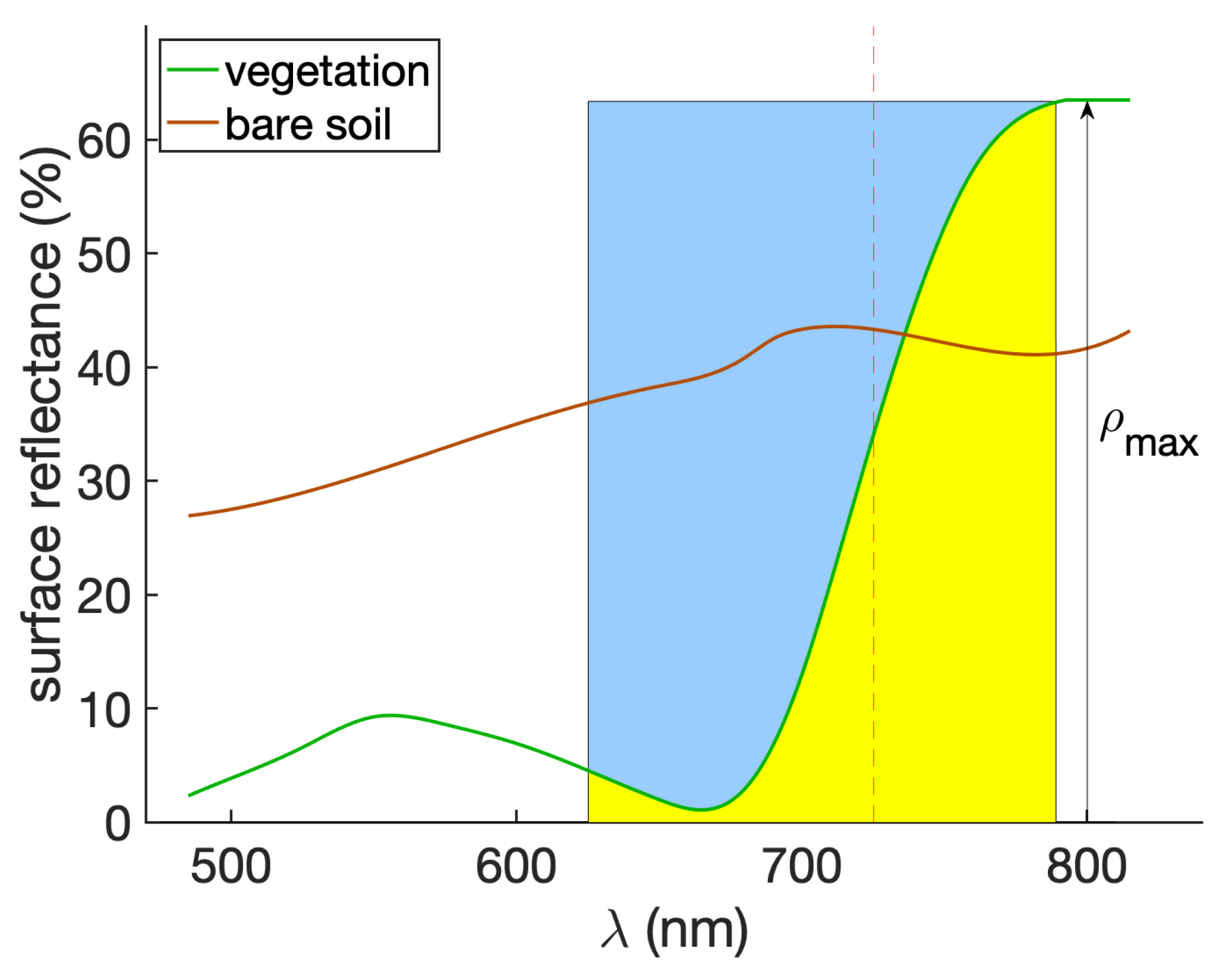
2.5. Extraction of Biophysical Parameters from HS and MS Data

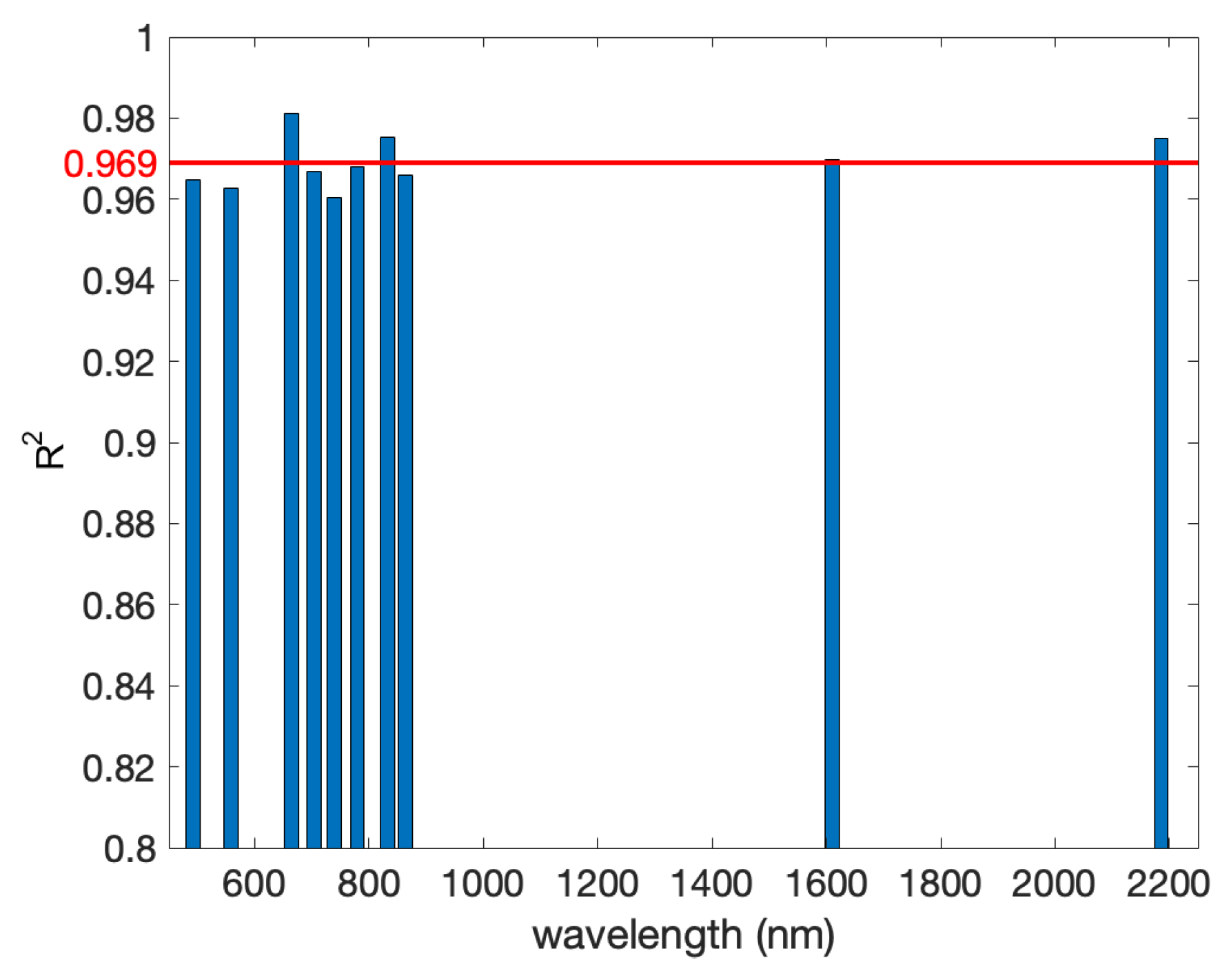
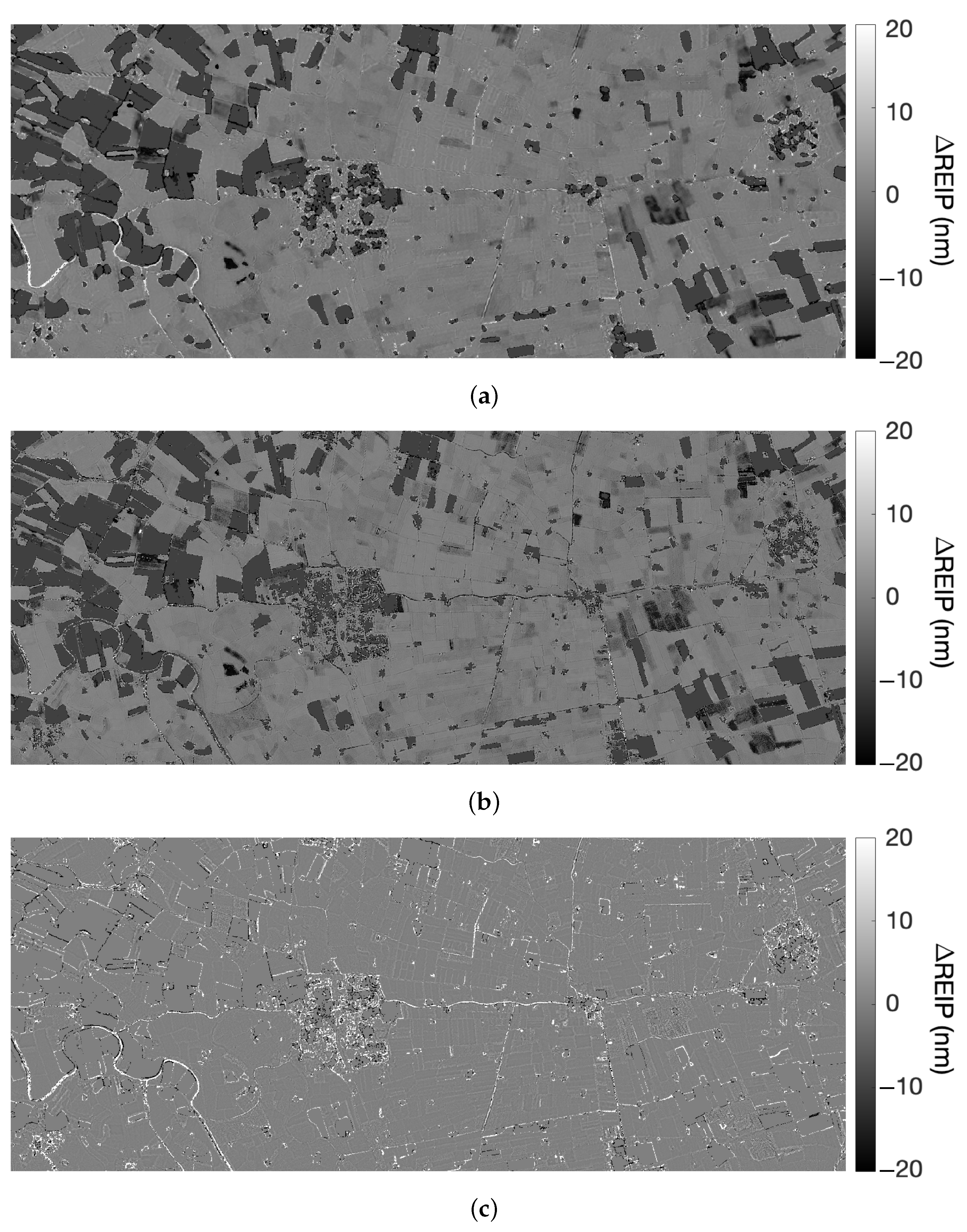
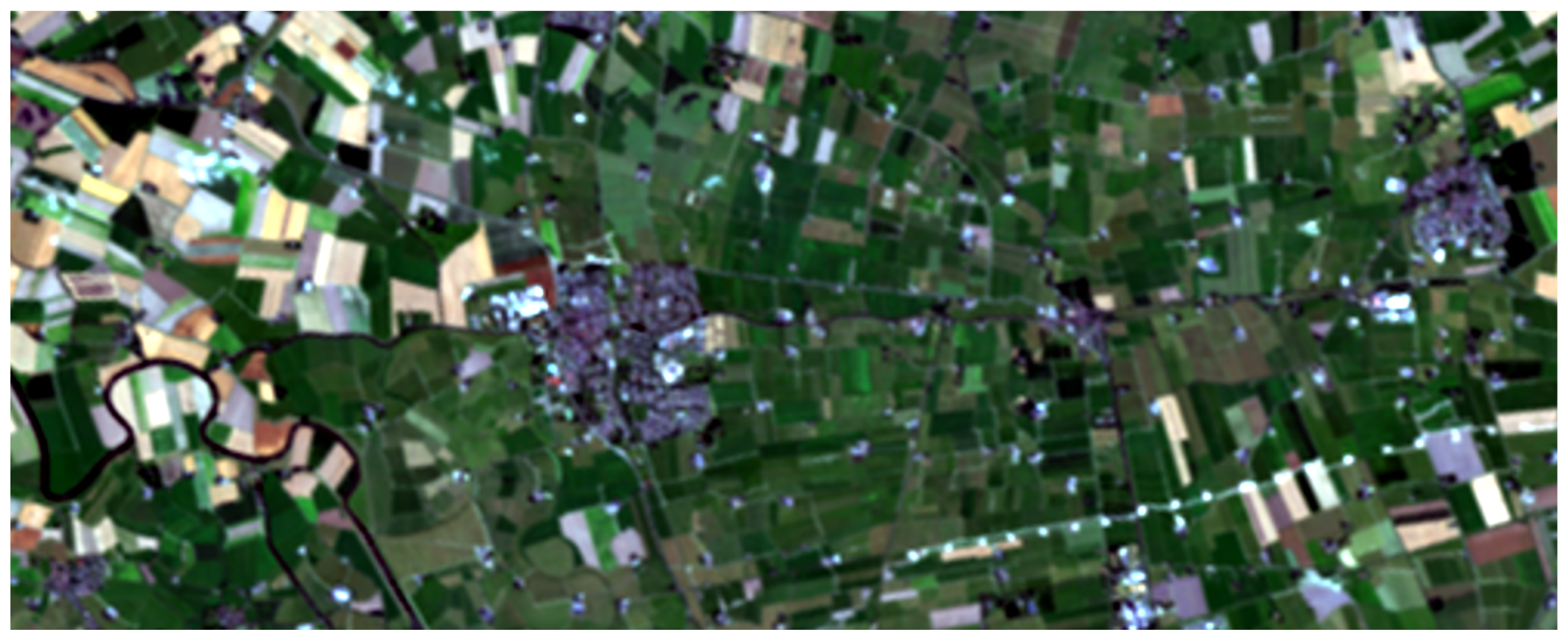
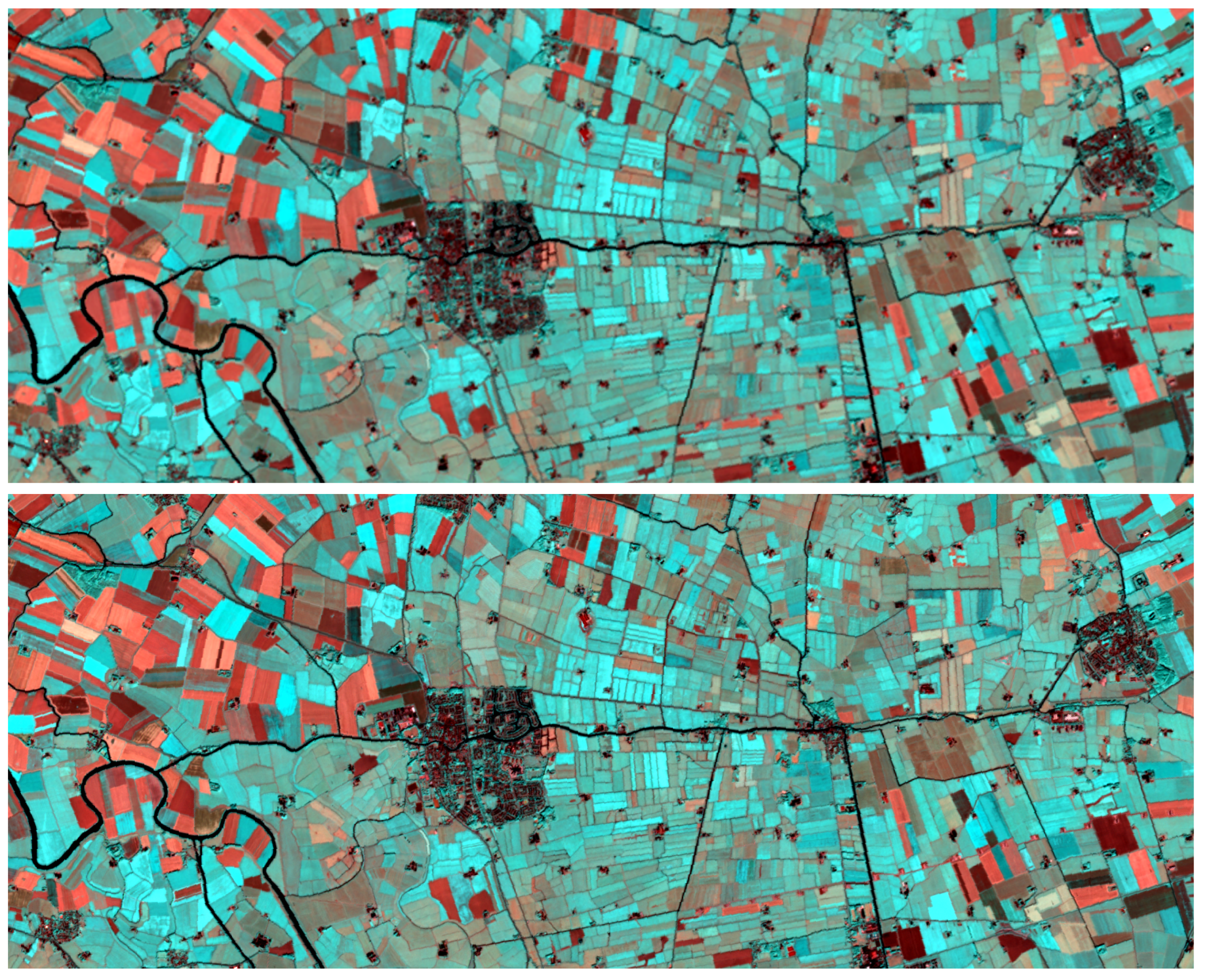
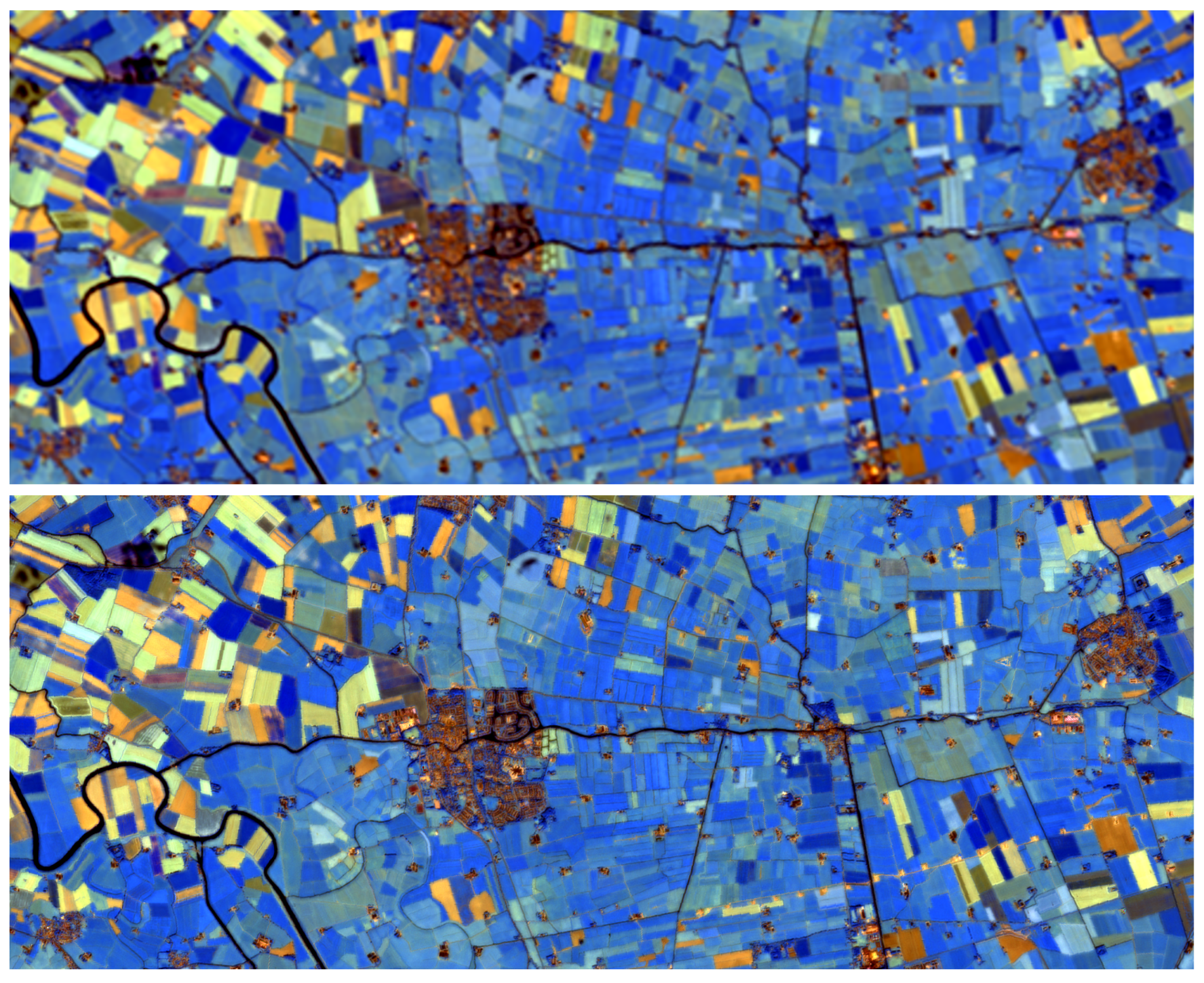
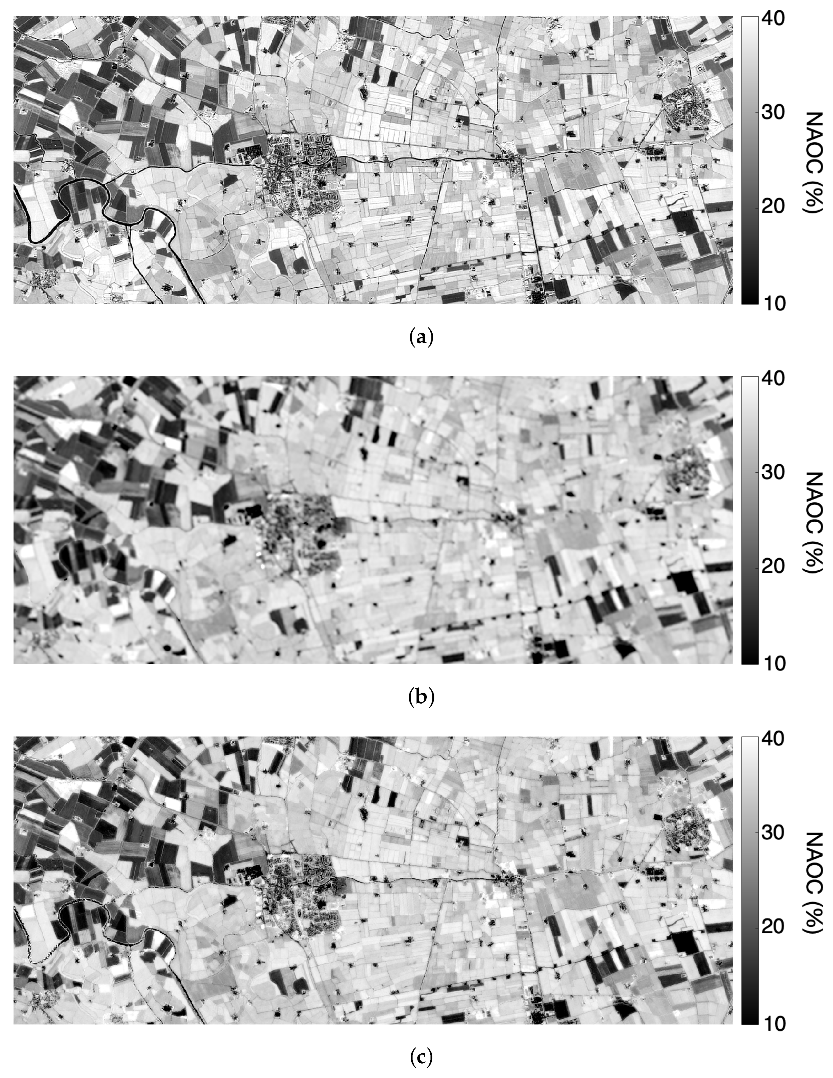
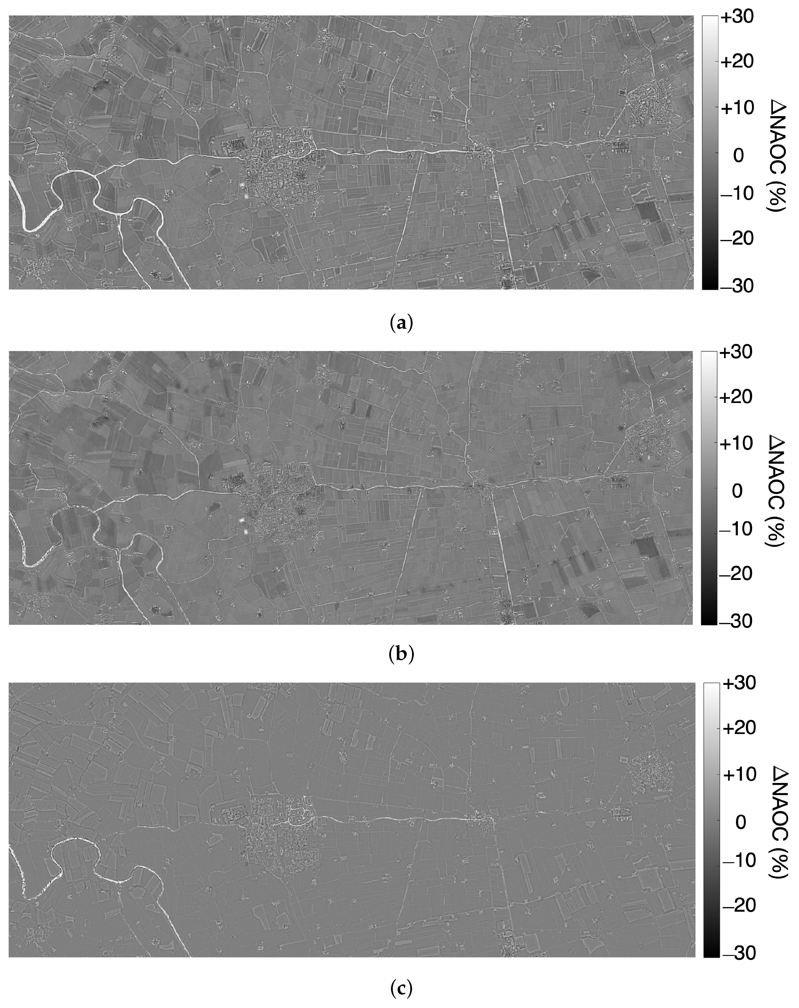
During the last decades, the extraction of biophysical parameters from crops has been translated from in-field measurements carried out by means of portable instruments to remote measurements performed by airborne and spaceborne MS/HS imaging instruments [33]. A great effort has been made to correlate in situ measurements with normalized indexes derived from multiband data [34]. As an example, LAI, which is a geometric parameter of crops and tree canopies, has been brought back to NDVI [35].

The definition and calculation of a spectral index suitable for characterizing vegetated landscapes depend on the number and widths of the bands of the imaging spectrometer. Here, we consider a couple of indexes that benefit from the availability of quasi-continuous pixel spectra: NAOC and REIP. An optical feature suitable for the analysis of vegetated areas, originally devised for HS data, having several bands in the (700–800) nm interval, is the normalized area over reflectance curve (NAOC) [2]:

$$\mathrm{NAOC}\triangleq 1-\frac{{\int }_{{\lambda }_{\mathrm{RED}}}^{{\lambda }_{\mathrm{NIR}}}\rho \left(\lambda \right)d\lambda }{{\rho }_{\mathrm{NIR}}·({\lambda }_{\mathrm{NIR}}-{\lambda }_{\mathrm{RED}})}$$

(7)

in which the integral can be calculated with any numerical algorithm, e.g., zero-order or linear approximation, from HS samples. Equation (7) represents the one complement of the integral of the surface reflectance function normalized to the product between the reflectance of the NIR channel and the difference in center wavelengths of the NIR and RED channels, as shown in Figure 3. The values of NAOC range in [0, 1] and are directly related to the chlorophyll content of the scene [2]. Hence, for sample spectra different from vegetation, e.g., bare soil, the values of NAOC are lower.

The definition of NAOC can be extended to Sentinel-2 data, thanks to the presence of the three RE bands. Equation (7) can be rewritten as:

$${\mathrm{NAOC}}_{\mathrm{S}2}=1-\frac{{\sum }_{i=4}^8{\rho }_i{\Delta }_{{\lambda }_i}}{{\rho }_8·{\sum }_{i=4}^8{\Delta }_{{\lambda }_i}},$$

(8)

in which ${\rho }_i$ is the surface reflectance of the ith band and the five bands used for NAOC calculation are described in

Table 1. Band name, spatial resolution, center wavelength, and spectral width of the Sentinel-2 bands used for NAOC and REIP calculation.

S2 Band	B4	B5	B6	B7	B8
resolution (m)	10	20	20	20	10
center $\lambda$ (nm)	665	705	740	783	842
$\Delta \lambda$ (nm)	30	15	15	20	115

.

All the data should be expressed as surface reflectance; haze-corrected spectral radiance, however, provides a good approximation, thanks to the normalization of the integral in Equation (7) and of the summation in Equation (8), which roughly removes the dependencies on solar irradiance and atmospheric transmittance [22].

Another vegetation index that takes advantage from the availability of a large number of spectral bands is the red-edge inflection point (REIP) [1]. In fact, the edge between the absorption and reflection regions of the spectrum is ideally located in the inflection point of the curve, in which the first-order derivative attains its maximum, or equivalently, the second-order derivative crosses the zero:

$$\mathrm{REIP}=arg\underset{\lambda \in \mathrm{RE}}{max}\left[\frac{d\rho \left(\lambda \right)}{d\lambda }\right],$$

(9)

in which the maximum is restricted to the RE interval, approximately [700, 800] nm. For HS data, the maximum of the first derivative or the zero-crossing of the second derivative are calculated by fitting a polynomial to the derivatives that have been calculated from spectral samples. The polynomial interpolation is necessary because the spectral sampling in the VNIR region of EnMAP is 6.5 nm, whereas the accuracy in the determination of REIP should be 1 nm or less.

For instruments with sparse bands, like Sentinel-2, a (quasi-)continuous spectrum is unavailable. Thus, approximations of REIP have been devised, like [3]

$${\mathrm{REIP}}_{S2}=c\lambda \left(B5\right)+[c\lambda \left(B6\right)-c\lambda \left(B5\right)]·\frac{\left[\rho \right(B4)+\rho (B7\left)\right]/2-\rho \left(B5\right)}{\rho \left(B6\right)-\rho \left(B5\right)},$$

(10)

in which the center wavelength ($c\lambda$) of the individual bands are replaced by the values in Table 1. In both Equations (9) and (10), REIP, also termed red-edge position (REP), is a wavelength expressed in nm. REIP is affected by biochemical and biophysical parameters and has been used to estimate leaf chlorophyll or nitrogen content [1].

We wish to remark that NAOC requires calculation of an integral of a surface reflectance spectrum; REIP, calculation of a derivative. Thus, the spectral sampling, more specifically, the number and widths of bands, is expected to be crucial for REIP, but not stringent for NAOC.

3. Results

3.1. Fusion Simulations

In a preliminary version of the present study [36], PRISMA and Sentinel-2 data have been fused together, without concern on possible applications to studies of vegetation. Here, the EnMAP dataset introduced in Section 2.1 will be hyper-sharpened by means of the Sentinel-2 dataset of the same area taken on the same day. Firstly, the consistency of the spectral signatures acquired by the HS (EnMAP) and MS (Sentinel-2) instruments is evidenced in Figure 4 and Figure 5, displaying RGB true-color compositions of the test area, as imaged from the two satellites. The original Level-2A data product is displayed at the native resolution for Sentinel-2, with an interpolation by a factor three for EnMAP. The match of color hues between the two images is impressive, thereby revealing that instrumental and atmospheric corrections were effectively performed, also because there is only an hour difference between the two acquisitions and thus a small difference in the solar elevation, which is easily corrected.

The results of the inner stage of hyper-sharpening carried out on Sentinel-2 data only are reported in Figure 6. Three 20 m bands in the upper RE, NIR, and SWIR wavelengths are hyper-sharpened at 10 m by means of the four 10 m VNIR bands. Besides the fidelity of color signatures, the increased sharpness, especially noticeable in the urban settlements, is impressive for a 2:1 scale ratio.

The results of the outer stage of hyper-sharpening concerning the 30 m original EnMAP data and 10 m Sentinel-2 bands, six of which have previously been hyper-sharpened at 10 m, are shown in Figure 7 for a color composition of bands spanning the empty gap of the MS instrument, if we exclude the 60 m bands that have not been considered in this study. The sharpening is now even more noticeable, because the scale ratio is 3:1 instead of 2:1. The geometric sharpness and spectral fidelity are even more surprising, because they come from separate datasets of different instruments, without any spectral overlap. We cannot help noticing the excellent spatial alignment of the two datasets, simply delivered in geocoded format, without any further geometric correction by users. The alignment is automatic, because the test site is perfectly flat.

Figure 8 shows that NRMSE is less than 2% in the NIR spectrum, around 3% in the visible wavelengths, and slightly higher than 2% in the right part of the reflective spectrum, with three pronounced peaks corresponding to the water vapor absorption and the rightmost edge of the SWIR interval, in which the quantum efficiency of the detector quickly decays. The absorption and detector inefficiency determine a marked decrement in the signal-to-noise ratio (SNR) and a loss of consistency of the fusion product to its noisy original. Nevertheless, NRMSE is practically always lower than 5% and lower than 3% on average, thereby indicating a good consistency of the fused HS data with the original ones. We wish to remind readers that the EnMAP dataset contains almost all the bands that have been acquired (213 over 224), thanks to an extremely dry acquisition day with very close pass times of the two satellites.

As shown in Figure 9, the trend of the spatial consistency index is rather flat, with the exception of small decrements towards the leftmost edge of the spectrum at 420 nm, due to quantum inefficiency, and around 700 nm, possibly due to instrumental corrections, because the first absorption wavelength in the VNIR spectrum occurs at approximately 760 nm. The average is close to 97.5% and indicates a high degree of spatial consistency. Again, the value of the index depends on the SNR of the original HS data, in the sense that low-SNR HS bands match the synthetic Pan to a lower extent.

The third and last index measures the inter-sensor consistency and is specific to the layout of spectral bands of Sentinel-2. The index reflects the ability of the hyper-sharpened EnMAP dataset to synthesize back the sharpening bands of Sentinel-2. With reference to Figure 10, the coefficient of determination, $R^2$, closely attains a unity value for all the bands of Sentinel-2. Interestingly, the bands that are better synthesized are the large bands, for which more information comes from the hyper-sharpened HS dataset: red, NIR, far SWIR, and near SWIR. Conversely, the consistency is lower for the narrower bands of the MS instrument: blue, green, the three RE, and the narrow-band NIR (see Figure 1). The lowest value of consistency is attained by the center RE band, of width 15 nm, which marks the spectral edge between absorption and reflection of vegetation. The average consistency, however, is 96.9%, with a peak of 98%. The values of the index for the four large bands lie above the mean; below the mean, for the six narrow bands. The three 60 m bands are not considered, because they are of no use for fusion with a 30 m HS dataset.

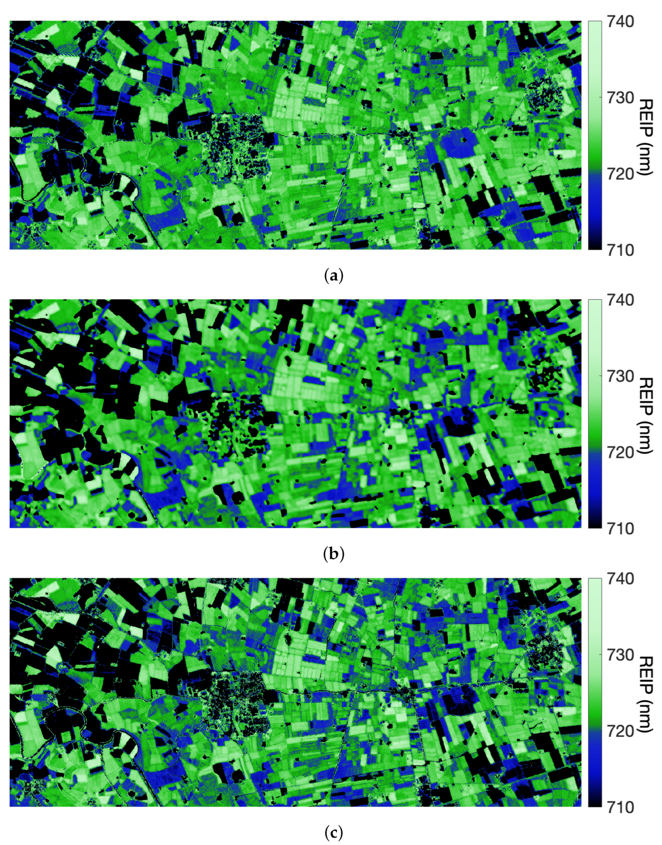
3.2. Extraction of Vegetation Indexes

The extraction of spectral indexes related to the biophysical status of vegetation will be carried out on the EnMAP dataset. In fact, notwithstanding that multitemporal observations of PRISMA have been recently used for studies on vegetation [37], the available PRISMA dataset features only 69 bands out of the 240 that are hypothetically available. The missing bands have been discarded by the data provider because of a number of inconveniences: high content of atmospheric water vapor that makes the bands around the absorption gaps of SWIR totally useless; temporary misfunctionings of several solid-state detectors that create striping artifacts; severe quantum inefficiency in proximity of the edges of each of the VNIR and SWIR spectrometers, such that the bands close to 400 nm and 2500 nm are extremely noisy (this effect is mitigated in the (1000,1100) nm region by the spectral overlap of the two instruments). For all these reasons, the test PRISMA dataset is suitable for pansharpening, but less so for hyper-sharpening, because the auxiliary Sentinel-2 dataset does not exhibit the same inconveniences; thus, the fusion of datasets from the two instruments may be unrewarding. Especially, the cross-consistency index reported in Figure 10 attains an average of about 0.6 for the PRISMA HS dataset. These reasons suggest that the hyper-sharpened PRISMA dataset described in [36] may not be suitable for physical investigations.

The first test concerns calculation of REIP from (a) hyper-sharpened Sentinel-2 data at 10 m; (b) original 30 m EnMAP data bicubically interpolated at 10 m; (c) EnMAP data hyper-sharpened at 10 m by means of the hyper-sharpened Sentinel-2 data at 10 m. The multiband dataset used for REIP calculation in case (c) is obtained by sharpening the dataset used for case (b) through the dataset used for case (a). Figure 11 shows, top to bottom, the map of REIP calculated as in case (a), (b), and (c), respectively. The map in case (a) exhibits a good geometrical accuracy, particular to the 10 m Sentinel-2 dataset. The map in case (b) is expected to be radiometrically accurate, because of the quasi-continuous spectra captured by the HS instrument, but appears to be geometrically coarse, because the original 30 m pixels contain mixed spectra of different landcovers. By comparing cases (a) and (b), the radiometric inaccuracy of (a), especially noticeable inside homogeneous regions with little vegetation, stands out, because REIP is calculated from only four bands, as in Equation (10). Instead, the REIP of the original HS data in case (b) is calculated by fitting a fourth-order polynomial to the first-order derivatives of the spectrum. However, the map lacks geometric sharpness at the edges of different fields with more or less vegetation. Eventually, REIP calculated from hyper-sharpened EnMAP data, shown in Figure 11c, trades off the accuracy inside homogeneous regions particular to case (b) and the geometric sharpness of the map noticeable in Figure 11a.

Figure 12a–c quantifies the difference in REIP for the following three cases: (a) is REIP of the original 30 m EnMAP interpolated to 10 m minus the REIP of hyper-sharpened Sentinel-2 at 10 m; (b) is REIP of hyper-sharpened EnMAP minus the REIP of 10 m Sentinel-2; (c) is the difference in REIP calculated from original and hyper-sharpened EnMAP data. Map (a) exhibits fair geometric quality, but mediocre radiometric accuracy: REIP is also often inaccurate inside vegetated patches. Map (b) reveals a good geometric accuracy but still a certain inaccuracy inside homogeneous regions. Map (c) highlights that the difference in REIP calculated from original and hyper-sharpened EnMAP data exhibits significant values only at the edges between fields and on textures, where the low spatial resolution of EnMAP cannot resolve mixed border pixels.

The results of NAOC, symmetrically shown in Figure 13a–c and Figure 14a–c, follow the same trend, with the slight difference that its calculation requires an integral and not a derivative of the spectrum. Thus, its accuracy is less crucial than that of REIP in the case of a low number of spectral samples.

The map of NAOC calculated from 10 m Sentinel-2 data is reasonably accurate, including radiometrically (see Figure 13a. The map in Figure 13b calculated from 30 m EnMap is a little sharp, but radiometrically accurate, since it has been derived from quasi-continuous pixel spectra. Figure 13c shows that the map calculated from hyper-sharpened EnMAP data is slightly less sharp than the map in Figure 13a, while retaining the radiometric accuracy of the map in Figure 13b.

Figure 14a–c reveals that the difference in NAOC progressively vanishes from case (a) to case (c). The advantage of hyper-sharpened EnMAP over original EnMAP is concentrated in the mixed border pixels. The integral, however, is less sensitive to the number of bands than the derivative. The effect of mixed pixels is also less pronounced, because NAOC is calculated on the whole spectrum in (700,800) nm, and REIP only on the rising front of the spectrum; thus, REIP experiences gross errors if the area is not fully vegetated.

To provide a deeper insight into the difference maps of Figure 12 and Figure 14, cumulative statistics of differences have been calculated on the disaggregated classes of spectrally pure and mixed pixels. The two classes have been separated by thresholding the map in Figure 14c. The mask of pure (black) and mixed (white) pixels is displayed in Figure 15. The same mask is used also for REIP, since the attribute of pure and mixed pixels is independent of the index that is being calculated.

The statistics of differences calculated on the disaggregated classes of pure and mixed pixel spectra are reported in

Table 2. RMS differences ${\Delta }_{\mathrm{NAOC}}$ and ${\Delta }_{\mathrm{REIP}}$ (nm) calculated on pure/mixed pixesl of the map in Figure 15 between (a) original 30 m EnMAP interpolated at 10 m and hyper-sharpened 10 m Sentinel-2; (b) hyper-sharpened 10 m EnMAP and hyper-sharpened 10 m Sentinel-2; (c) original 30 m EnMAP interpolated at 10 m and hyper-sharpened 10 m EnMAP.

(a)	${\mathbf{\Delta }}_{\mathbf{NAOC}}$	${\mathbf{\Delta }}_{\mathbf{REIP}}$	(b)	${\mathbf{\Delta }}_{\mathbf{NAOC}}$	${\mathbf{\Delta }}_{\mathbf{REIP}}$	(c)	${\mathbf{\Delta }}_{\mathbf{NAOC}}$	${\mathbf{\Delta }}_{\mathbf{REIP}}$
pure	0.013	4.48	pure	0.012	4.41	pure	0.003	0.79
mixed	0.034	16.78	mixed	0.019	16.58	mixed	0.011	3.74

. The three cases (a), (b), and (c) correspond to the three maps in Figure 12a–c and Figure 14a–c. A series of considerations can be made. With specific reference to case (c), on pure pixels the advantage of fusion of HS data is limited. The average RMS difference is 0.3% for NAOC and 0.79 nm for REIP. The latter value is presumably below the sensitivity threshold of REIP, because the spectral spacing of EnMAP data is 6.5 nm, the sensitivity depends on the intrinsic noise of the instrument, and REIP is a differential parameter highly influenced by the noise. On mixed pixels, both differences significantly grow, less than four times for NAOC, more than four times for REIP. The conclusion is that there is a significant advantage of using fused HS data on mixed pixels, whereas on pure pixels 30 m EnMAP may be adequate. The cases in which original EnMAP (a) and fused EnMAP (b) are compared to hyper-sharpened Sentinel-2 are quite similar, almost identical in terms of REIP differences. What immediately stands out is that NAOC is scarcely influenced by the number of bands of the two instruments. Whether fifteen bands of EnMAP, either original or sharpened, or five bands of Sentinel-2 (see Equation (8)) are used, the RMS difference is reasonably small: on pure pixels, 1.3% for original EnMAP, 1.2% for fused EnMAP. The decreasing trend is emphasized on mixed pixels: 3.4% for original EnMAP, 1.9% for fused EnMAP. The extremely high values of REIP differences entail a series of considerations. REIP is very sensitive to the spectral sampling. The bands of Sentinel-2 are not equally spaced and Equation (10) is an approximation [3] that considers the positions and widths of four bands (red and the three REs). The equally sampled spectra of EnMAP, both original and sharpened, expedite calculation of the first-order derivative and its polynomial approximation to find the maximum. Thus, also in the presence of pure pixels, there is a difference greater than 4 nm between REIP calculated from Sentinel-2 data and from EnMAP data, either sharpened or not. On mixed pixels such a difference grows to over 16 nm because, besides the insufficient number of bands, the spectra of mixed pixels may deviate from the sigmoid shape of vegetation spectra, to which the inflection point applies. In this analysis, the true values of NAOC and REIP are unknown, but they can be inferred from the twelve cases reported in Table 2. The true value of NAOC is that measured on sharpened EnMAP data on all pixels. The true value of REIP is presumably close to the average of the values calculated on original and sharpened EnMAP data on pure pixels; the value calculated on mixed pixels is most likely close to that of sharpened EnMAP data. The average is introduced because on pure pixels, original and sharpened EnMAP spectra are noisy observations of the same stochastic process, in the sense that the spatial enhancement changes the realization of the noise already present in the original data. Thus, the average is expected to reduce the influence of the noise on spectra that are substantially both correct.

4. Discussion

The importance for studies on vegetation of the fusion of an HS dataset with an MS dataset having greater spatial (and temporal) resolution lies in the possibility of unmixing pixel spectra to obtain more accurate estimates of biochemical and biophysical parameters in the presence of spatial discontinuities in the vegetation cover. For boundless fields and forests, at a 30 m scale, the fraction of mixed pixels tends to zero. Nevertheless, we have shown that the fused spectra of pure pixels are as accurate as those of the original HS dataset. The analysis reported in this study can also be conducted on other vegetation indexes calculated from measured spectra of fused datasets and are not particular to specific HS and MS instruments. Our goal is to evaluate our sharpening procedure not only through statistical indexes, but also for a possible application context.

Favorable weather conditions lead to the suppression of thirteen bands only. Less-favorable conditions, particularly a high content of water vapor in the atmosphere, can increase the number of bands that must be suppressed. In the case of clouds, both instruments are unable to image the Earth’s surface. Fortunately, all the bands that are suppressed due to meteorological conditions during acquisition are located in the SWIR wavelengths, seldom used for vegetation analysis. Though the test site is perfectly flat, the problem of hilly, mountainous, or even rugged terrain is brought back to geometric corrections, which are made by the data provider and would require a digital elevation model (DEM) of proper spatial sampling. For 30 m and 10 m data, a DEM at 10 m, as used for data at metric resolution, is generally more than adequate. The conversion from spectral radiance (L1 product) to surface reflectance (L2 product) includes the correction of solar irradiance, which requires knowledge of the illumination geometry and hence, the availability of a DEM of adequate resolution. All these issues are independent of the fusion algorithm, which, in turn, may be little effective if the data are not properly corrected. Geometric corrections are especially crucial. Inaccurate atmospheric corrections may be tolerated if normalized indexes, typically NAOC, are calculated. Inaccurate corrections of the datasets are likely to impair the fusion success and may be detected by abnormally low values of the statistical indexes in Figure 9 and Figure 10.

The proposed approach may be useful for the temporal monitoring of vegetation [1,38], thanks to the regular availability of Sentinel-2 datasets every five days. Conversely, HS satellite observations are on-demand; hence, expensive and necessarily sparse over time, also because of adverse meteorological conditions that may delay the planned acquisition. In principle, it would be possible to transplant the temporal repetition capability of Sentinel-2 MS data into the spectral resolution of HS data to obtain many fused HS observations with only a few original HS datasets. Analogously to the fusion of Sentinel-2 and Sentinel-3 data [39], the fusion of EnMAP with Sentinel-2 would achieve an increase in both spatial and temporal resolutions. In a likely scenario, HS datasets are required only for substantial changes in the vegetated landcover, more or less spaced in time, depending on the phenology of vegetation. Sentinel-2 datasets can be freely downloaded every five days, though moderate cloud cover may limit their usability on some dates. The goal is to associate a group of Sentinel-2 images with a unique HS dataset and produce as many hyper-sharpened HS datasets as there are MS datasets. There are no problems of spatial overlap, because the swath of Sentinel-2 is ten times larger than that of any HS satellite instrument. The sole extra task, which can be performed by experts or automatized, is the association of a temporarily contiguous segment of MS datasets with a unique HS dataset. Then, the latter is hyper-sharpened by means of each of the MS dataset of its group. Whenever the number of HS datasets of the same scene is low, also in the presence of critical phenological changes, it would be preferable to create as many HS datasets as there are MS ones. The temporal interpolation of the temporally rare HS pixel spectra should be driven by the phenological evolution of the scene, which in principle can be estimated from the MS spectra, coarsely sampled in wavelength, but more frequently in time. After that, the fusion is one-to-one: one true MS dataset shall sharpen one HS dataset, either true or interpolated, exactly as described in the present study.

5. Conclusions

We have shown that an HS observation can be merged with an auxiliary MS observation of the same scene of greater spatial resolution taken at approximately the same date and time. The presence of Pan together with either the HS image or the MS image entails a further pansharpening step. Nowadays, satellite HS missions provide approximately 220 narrow spectral bands at a 30 m spatial scale. The ideal auxiliary MS dataset is provided by the Sentinel-2 twin-satellite constellation, with 10 m, 20 m, and 60 m spectral bands and a repetition capability of five days. Thus, EnMAP datacubes can be upgraded to 10 m resolution by means of two nested hyper-sharpening steps, the former performed on Sentinel-2 data only to bring all its bands to 10 m, the latter on 30 m HS data that have been brought to 10 m. For EnMAP data, where the Pan image is missing, statistical inter-sensor consistency indexes have been developed to measure the improvement of the fused data over the original EnMAP and Sentinel-2 data.

After the consistency check has validated the hyper-sharpened dataset, we can calculate vegetation indexes that take advantage of equally spaced fine samples from the sharpened data. The accuracy of REIP and NAOC calculated from fused HS data is analyzed on the two classes of pure and mixed pixels. On pure pixels, the values of REIP and NAOC calculated from the fused data are consistent with those calculated from the original HS data. Conversely, thanks to hyper-sharpening, mixed pixels are spectrally unmixed to resolve the 10 m scale of the MS data. Wherever mixed pixels are rare, e.g., in the Amazon forest or in the boundless wheat fields of Canada, the proposed method may be of limited usefulness.

The results of the proposed procedure are obtained with real-time processing, do not require parametric adjustments and/or training datasets, and are fully reproducible. We wish to remind readers that accurate instrumental, geometric, and atmospheric corrections are mandatory for the success of multi-platform hyper-sharpening. Therefore, for images of rugged terrain, the geometric alignment of the datasets may be crucial. The accuracy of atmospheric correction is less stringent, at least for NAOC and REIP, because the former is normalized; the latter, being an inflection point, is little sensitive to small changes in gain and offset that lead from the spectral radiance to surface reflectance format [21]. For the available HS dataset described in [36], the new consistency indexes described in this study yield less-than-mediocre results, even when the same fusion algorithm and auxiliary sensor dataset are used. This fact suggests that the intrinsic quality of a dataset may be brought back to its consistency with another dataset of trustful quality.

References

1. Cho, M.A.; Skidmore, A.K. A new technique for extracting the red edge position from hyperspectral data: The linear extrapolation method. Remote Sens. Environ. 2006, 101, 181–193. [Google Scholar] [CrossRef]
2. Delegido, J.; Alonso, L.; González, G.; Moreno, J. Estimating chlorophyll content of crops from hyperspectral data using a normalized area over reflectance curve (NAOC). Int. J. Appl. Earth Obs. Geoinf. 2010, 12, 165–174. [Google Scholar] [CrossRef]
3. Herrmann, I.; Pimstein, A.; Karnieli, A.; Cohen, Y.; Alchanatis, V.; Bonfil, D. LAI assessment of wheat and potato crops by VENµS and Sentinel-2 bands. Remote Sens. Environ. 2011, 115, 2141–2151. [Google Scholar] [CrossRef]
4. Vivone, G. Multispectral and hyperspectral image fusion in remote sensing: A survey. Inform. Fusion 2023, 89, 405–417. [Google Scholar] [CrossRef]
5. Alparone, L.; Aiazzi, B.; Baronti, S.; Garzelli, A. Remote Sensing Image Fusion; CRC Press: Boca Raton, FL, USA, 2015. [Google Scholar]
6. Selva, M.; Aiazzi, B.; Butera, F.; Chiarantini, L.; Baronti, S. Hyper-sharpening: A first approach on SIM-GA data. IEEE J. Sel. Top. Appl. Earth Obs. Remote Sens. 2015, 8, 3008–3024. [Google Scholar] [CrossRef]
7. Aiazzi, B.; Alparone, L.; Baronti, S.; Lastri, C. Crisp and fuzzy adaptive spectral predictions for lossless and near-lossless compression of hyperspectral imagery. IEEE Geosci. Remote Sens. Lett. 2007, 4, 532–536. [Google Scholar] [CrossRef]
8. Karoui, M.S.; Deville, Y.; Benhalouche, F.Z.; Boukerch, I. Hypersharpening by joint-criterion nonnegative matrix factorization. IEEE Geosci. Remote Sens. Lett. 2017, 55, 1660–1670. [Google Scholar] [CrossRef]
9. Selva, M.; Santurri, L.; Baronti, S. Improving hypersharpening for WorldView-3 data. IEEE Geosci. Remote Sens. Lett. 2019, 16, 987–991. [Google Scholar] [CrossRef]
10. Lu, X.; Zhang, J.; Yu, X.; Tang, W.; Li, T.; Zhang, Y. Hyper-sharpening based on spectral modulation. IEEE J. Sel. Top. Appl. Earth Obs. Remote Sens. 2019, 12, 1534–1548. [Google Scholar] [CrossRef]
11. Restaino, R.; Vivone, G.; Addesso, P.; Chanussot, J. Hyperspectral sharpening approaches using satellite multiplatform data. IEEE Trans. Geosci. Remote Sens. 2021, 59, 578–596. [Google Scholar] [CrossRef]
12. Sihvonen, T.; Duma, Z.S.; Haario, H.; Reinikainen, S.P. Spectral profile partial least-squares (SP-PLS): Local multivariate pansharpening on spectral profiles. ISPRS Open J. Photogramm. Remote Sens. 2023, 10, 100049. [Google Scholar] [CrossRef]
13. Johnson, B. Effects of pansharpening on vegetation indices. ISPRS Int. J. Geo-Inf. 2014, 3, 507–522. [Google Scholar] [CrossRef]
14. Garzelli, A.; Aiazzi, B.; Alparone, L.; Lolli, S.; Vivone, G. Multispectral pansharpening with radiative transfer-based detail-injection modeling for preserving changes in vegetation cover. Remote Sens. 2018, 10, 1308. [Google Scholar] [CrossRef]
15. Middleton, E.M.; Campbell, P.K.E.; Ong, L.; Landis, D.R.; Zhang, Q.; Neigh, C.S.; Huemmrich, K.F.; Ungar, S.G.; Mandl, D.J.; Frye, S.W.; et al. Hyperion: The first global orbital spectrometer, earth observing-1 (EO-1) satellite (2000–2017). In Proceedings of the 2017 IEEE International Geoscience and Remote Sensing Symposium (IGARSS), Fort Worth, TX, USA, 23–28 July 2017; pp. 3039–3042. [Google Scholar] [CrossRef]
16. Cogliati, S.; Sarti, F.; Chiarantini, L.; Cosi, M.; Lorusso, R.; Lopinto, E.; Miglietta, F.; Genesio, L.; Guanter, L.; Damm, A.; et al. The PRISMA imaging spectroscopy mission: Overview and first performance analysis. Remote Sens. Environ. 2021, 262, 112499. [Google Scholar] [CrossRef]
17. Storch, T.; Honold, H.P.; Chabrillat, S.; Habermeyer, M.; Tucker, P.; Brell, M.; Ohndorf, A.; Wirth, K.; Betz, M.; Kuchler, M.; et al. The EnMAP imaging spectroscopy mission towards operations. Remote Sens. Environ. 2023, 294, 113632. [Google Scholar] [CrossRef]
18. Aguirre-Gutiérrez, J.; Rifai, S.; Shenkin, A.; Oliveras, I.; Bentley, L.P.; Svátek, M.; Girardin, C.A.; Both, S.; Riutta, T.; Berenguer, E.; et al. Pantropical modelling of canopy functional traits using Sentinel-2 remote sensing data. Remote Sens. Environ. 2021, 252, 112122. [Google Scholar] [CrossRef]
19. Aiazzi, B.; Alparone, L.; Garzelli, A.; Santurri, L. Blind correction of local misalignments between multispectral and panchromatic images. IEEE Geosci. Remote Sens. Lett. 2018, 15, 1625–1629. [Google Scholar] [CrossRef]
20. Aiazzi, B.; Alparone, L.; Baronti, S.; Garzelli, A.; Selva, M. Advantages of Laplacian pyramids over ”à trous” wavelet transforms for pansharpening of multispectral images. In Proceedings of the Image and Signal Processing for Remote Sensing XVIII; Bruzzone, L., Ed.; International Society for Optics and Photonics; SPIE: Bellingham, WA, USA, 2012; Volume 8537, pp. 12–21. [Google Scholar] [CrossRef]
21. Arienzo, A.; Aiazzi, B.; Alparone, L.; Garzelli, A. Reproducibility of pansharpening methods and quality indexes versus data formats. Remote Sens. 2021, 13, 4399. [Google Scholar] [CrossRef]
22. Pacifici, F.; Longbotham, N.; Emery, W.J. The importance of physical quantities for the analysis of multitemporal and multiangular optical very high spatial resolution images. IEEE Trans. Geosci. Remote Sens. 2014, 52, 6241–6256. [Google Scholar] [CrossRef]
23. Lolli, S.; Di Girolamo, P. Principal component analysis approach to evaluate instrument performances in developing a cost-effective reliable instrument network for atmospheric measurements. J. Atmos. Ocean. Technol. 2015, 32, 1642–1649. [Google Scholar] [CrossRef]
24. Lolli, S.; Sauvage, L.; Loaec, S.; Lardier, M. EZ LidarTM: A new compact autonomous eye-safe scanning aerosol Lidar for extinction measurements and PBL height detection. Validation of the performances against other instruments and intercomparison campaigns. Opt. Pura Apl. 2011, 44, 33–41. [Google Scholar]
25. Ciofini, M.; Lapucci, A.; Lolli, S. Diffractive optical components for high power laser beam sampling. J. Opt. Pure Appl. Opt. 2003, 5, 186–191. [Google Scholar] [CrossRef]
26. Chavez, P.S., Jr. Image-based atmospheric corrections–Revisited and improved. Photogramm. Eng. Remote Sens. 1996, 62, 1025–1036. [Google Scholar]
27. Fu, Q.; Liou, K.N. On the correlated k-distribution method for radiative transfer in nonhomogeneous atmospheres. J. Atmos. Sci. 1992, 49, 2139–2156. [Google Scholar] [CrossRef]
28. Aiazzi, B.; Alparone, L.; Argenti, F.; Baronti, S. Wavelet and pyramid techniques for multisensor data fusion: A performance comparison varying with scale ratios. In Proceedings of the Image and Signal Processing for Remote Sensing V; Serpico, S.B., Ed.; International Society for Optics and Photonics; SPIE: Bellingham, WA, USA, 1999; Volume 3871, pp. 251–262. [Google Scholar] [CrossRef]
29. Palsson, F.; Sveinsson, J.R.; Ulfarsson, M.O.; Benediktsson, J.A. Quantitative quality evaluation of pansharpened imagery: Consistency versus synthesis. IEEE Trans. Geosci. Remote Sens. 2016, 54, 1247–1259. [Google Scholar] [CrossRef]
30. Guan, X.; Li, F.; Zhang, X.; Ma, M.; Mei, S. Assessing full-resolution pansharpening quality: A comparative study of methods and measurements. IEEE J. Sel. Top. Appl. Earth Obs. Remote Sens. 2023, 16, 6860–6875. [Google Scholar] [CrossRef]
31. Arienzo, A.; Vivone, G.; Garzelli, A.; Alparone, L.; Chanussot, J. Full-resolution quality assessment of pansharpening: Theoretical and hands-on approaches. IEEE Geosci. Remote Sens. Mag. 2022, 10, 2–35. [Google Scholar] [CrossRef]
32. Alparone, L.; Garzelli, A.; Vivone, G. Spatial consistency for full-scale assessment of pansharpening. In Proceedings of the 2018 IEEE International Geoscience and Remote Sensing Symposium (IGARSS), Valencia, Spain, 22–27 July 2018; pp. 5132–5134. [Google Scholar]
33. Thenkabail, P.S.; Smith, R.B.; De Pauw, E. Hyperspectral vegetation indices and their relationships with agricultural crop characteristics. Remote Sens. Environ. 2000, 71, 158–182. [Google Scholar] [CrossRef]
34. Miraglio, T.; Adeline, K.; Huesca, M.; Ustin, S.; Briottet, X. Assessing vegetation traits estimates accuracies from the future SBG and biodiversity hyperspectral missions over two Mediterranean forests. Int. J. Remote Sens. 2022, 43, 3537–3562. [Google Scholar] [CrossRef]
35. Liang, L.; Di, L.; Zhang, L.; Deng, M.; Qin, Z.; Zhao, S.; Lin, H. Estimation of crop LAI using hyperspectral vegetation indices and a hybrid inversion method. Remote Sens. Environ. 2015, 165, 123–134. [Google Scholar] [CrossRef]
36. Garzelli, A.; Zoppetti, C.; Arienzo, A.; Alparone, L. Spatial resolution enhancement of PRISMA hyperspectral data via nested hypersharpening with Sentinel-2 multispectral data. In Proceedings of the 2023 IEEE International Geoscience and Remote Sensing Symposium, Pasadena, CA, USA, 16–21 July 2023; pp. 5997–6000. [Google Scholar] [CrossRef]
37. Tagliabue, G.; Boschetti, M.; Bramati, G.; Candiani, G.; Colombo, R.; Nutini, F.; Pompilio, L.; Rivera-Caicedo, J.P.; Rossi, M.; Rossini, M.; et al. Hybrid retrieval of crop traits from multi-temporal PRISMA hyperspectral imagery. ISPRS J. Photogramm. Remote Sens. 2022, 187, 362–377. [Google Scholar] [CrossRef] [PubMed]
38. Zhou, J.; Chen, J.; Chen, X.; Zhu, X.; Qiu, Y.; Song, H.; Rao, Y.; Zhang, C.; Cao, X.; Cui, X. Sensitivity of six typical spatiotemporal fusion methods to different influential factors: A comparative study for a normalized difference vegetation index time series reconstruction. Remote Sens. Environ. 2021, 252, 112130. [Google Scholar] [CrossRef]
39. Wang, Q.; Atkinson, P.M. Spatio-temporal fusion for daily Sentinel-2 images. Remote Sens. Environ. 2018, 204, 31–42. [Google Scholar] [CrossRef]
Figure 1. Sentinel-2 layout of spectral bands.
Remotesensing 16 00875 g001
Figure 2. Flow diagram of the proposed HS/Sentinel-2 sharpening method.
Remotesensing 16 00875 g002
Figure 3. Illustration of NAOC and REIP for two spectra. The blue area is the NAOC of vegetation. The inflection point (REIP), in which the spectrum of vegetation attains the maximum of its slope, is visible at approximately 730 nm. Maximum reflectance, ρ m a x , is attained in the NIR wavelengths.
Remotesensing 16 00875 g003
Figure 4. 15 km × 6 km EnMAP acquisition: 647-551-468 nm true-color composition at 30 m SSI, interpolated at 10 m.
Remotesensing 16 00875 g004
Figure 5. 15 km × 6 km Sentinel-2B acquisition: bands B4-B3-B2 as true-color composition at their original 10 m SSI.
Remotesensing 16 00875 g005
Figure 6. B11-B8a-B7 Sentinel-2 compositions: 20 m originals interpolated (top) at 10 m and hyper-sharpened (bottom) at 10 m.
Remotesensing 16 00875 g006
Figure 7. 2105,1707,1004 nm EnMAP compositions: (top) interpolated 30 m original; (bottom) hyper-sharpened at 10 m.
Remotesensing 16 00875 g007
Figure 8. Spectral consistency of EnMAP–Groningen: RMSE between original EnMAP bands and de-sharpened hyper-sharpened bands, normalized to the mean of the original band and plotted versus the wavelength.
Remotesensing 16 00875 g008
Figure 9. Spatial consistency of EnMAP–Groningen towards the sharpening Sentinel-2 data: coefficient of determination of the multivariate regression of the hyper-sharpened HS bands to the sharpening combination of hyper-sharpened MS band, plotted versus the wavelength. The average value, drawn in red, is 0.974.
Remotesensing 16 00875 g009
Figure 10. Spectral consistency of EnMAP–Groningen towards the sharpening Sentinel-2 bands: coefficient of determination of the multivariate regression of the hyper-sharpened HS bands to the hyper-sharpened MS band of Sentinel-2. The average value, drawn in red, is 0.969.
Remotesensing 16 00875 g010
Figure 11. Maps of REIP (nm) calculated from: (a) original S-2 hyper-sharpened at 10 m; (b) original 30 m EnMAP; (c) 30 m EnMAP hyper-sharpened at 10 m by 10 m hyper-sharpened Sentinel-2.
Remotesensing 16 00875 g011
Figure 12. Differences of REIP (nm): (a) original 30 m EnMAP interpolated at 10 m minus hyper-sharpened Sentinel-2 at 10 m; (b) EnMAP hyper-sharpened at 10 m minus Sentinel-2 at 10 m; (c) original 30 m EnMAP interpolated at 10 m minus EnMAP hyper-sharpened at 10 m.
Remotesensing 16 00875 g012
Figure 13. Maps of NAOC calculated from: (a) original S-2 hyper-sharpened at 10 m; (b) original 30 m EnMAP; (c) 30 m EnMAP hyper-sharpened at 10 m by 10 m hyper-sharpened Sentinel-2.
Remotesensing 16 00875 g013
Figure 14. Difference of NAOC: (a) original 30 m EnMAP interpolated at 10 m minus hyper-sharpened Sentinel-2 at 10 m; (b) EnMAP hyper-sharpened at 10 m minus Sentinel-2 at 10 m; (c) original 30 m EnMAP interpolated at 10 m minus EnMAP hyper-sharpened at 10 m.
Remotesensing 16 00875 g014
Figure 15. Mask of pixels with mixed spectra obtained by thresholding the map in Figure 14c.
Remotesensing 16 00875 g015