
Effects of Solar Intrusion on the Calibration of the Metop-C Advanced Microwave Sounding Unit-A2 Channels


Abstract
1. Introduction
2. Calibration Equation and Operational Processing
3. Anomalous Features in AMSU-A2 Blackbody Calibration Target
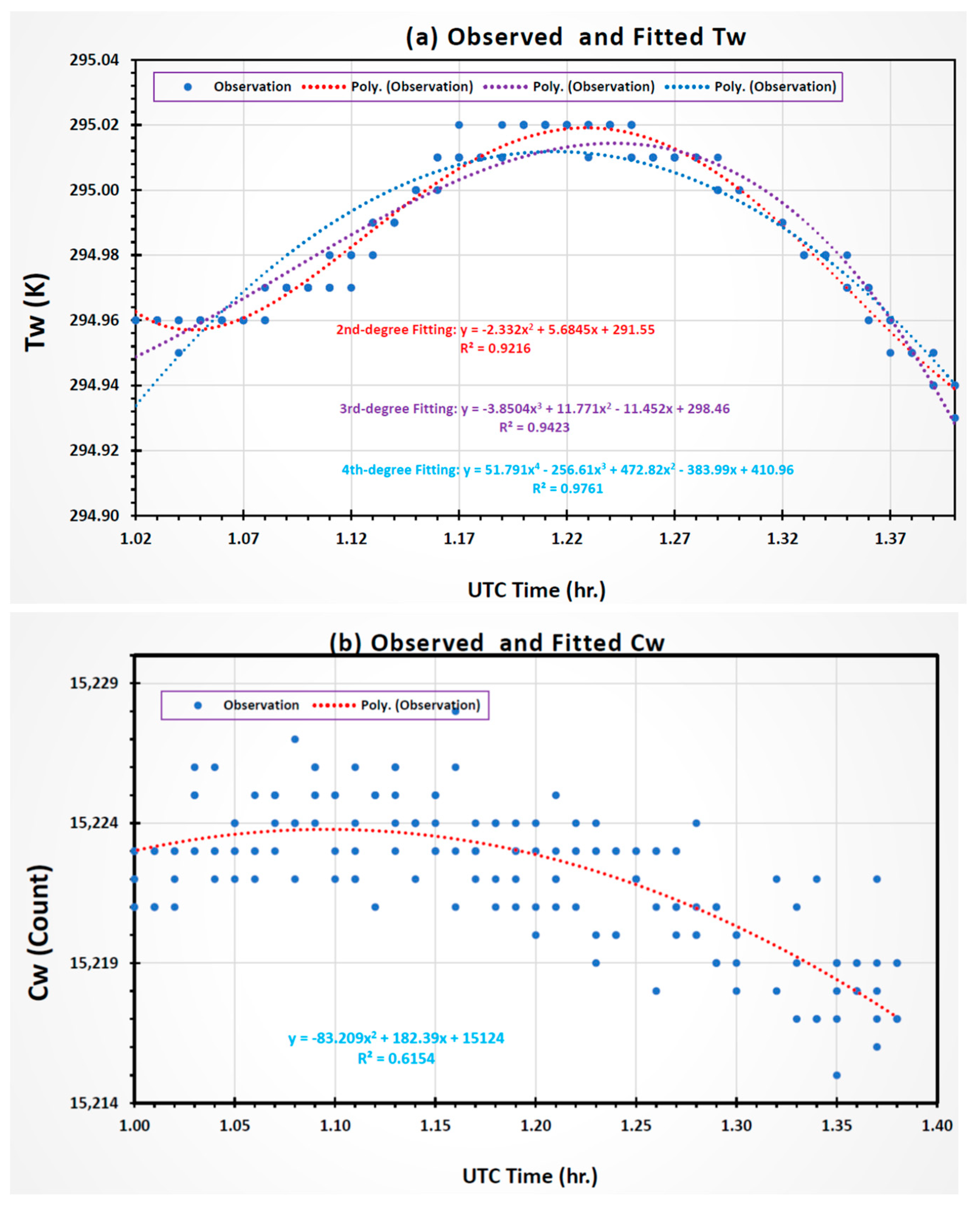
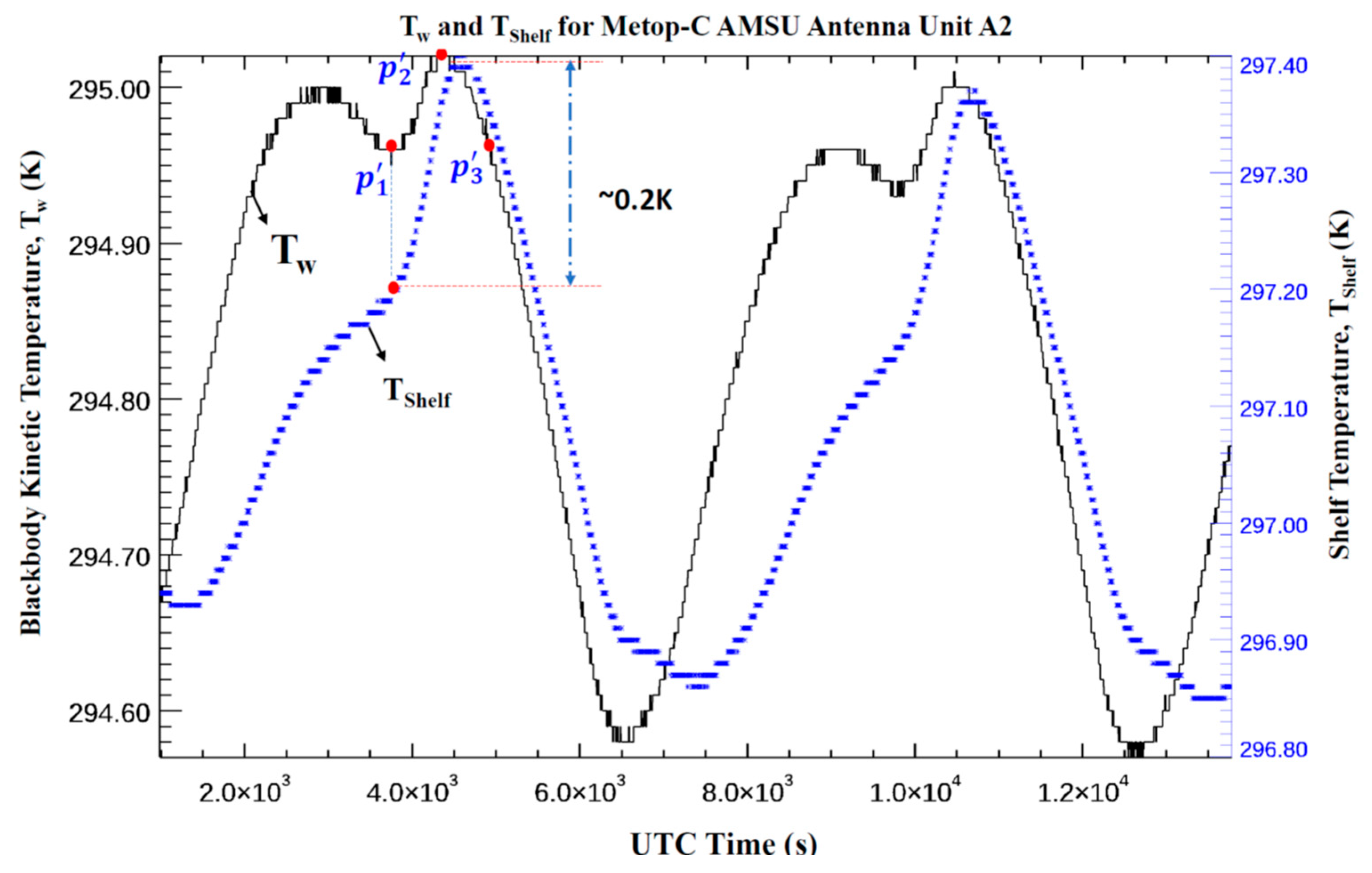
3.1. Anomalous Features
3.2. More Discussions
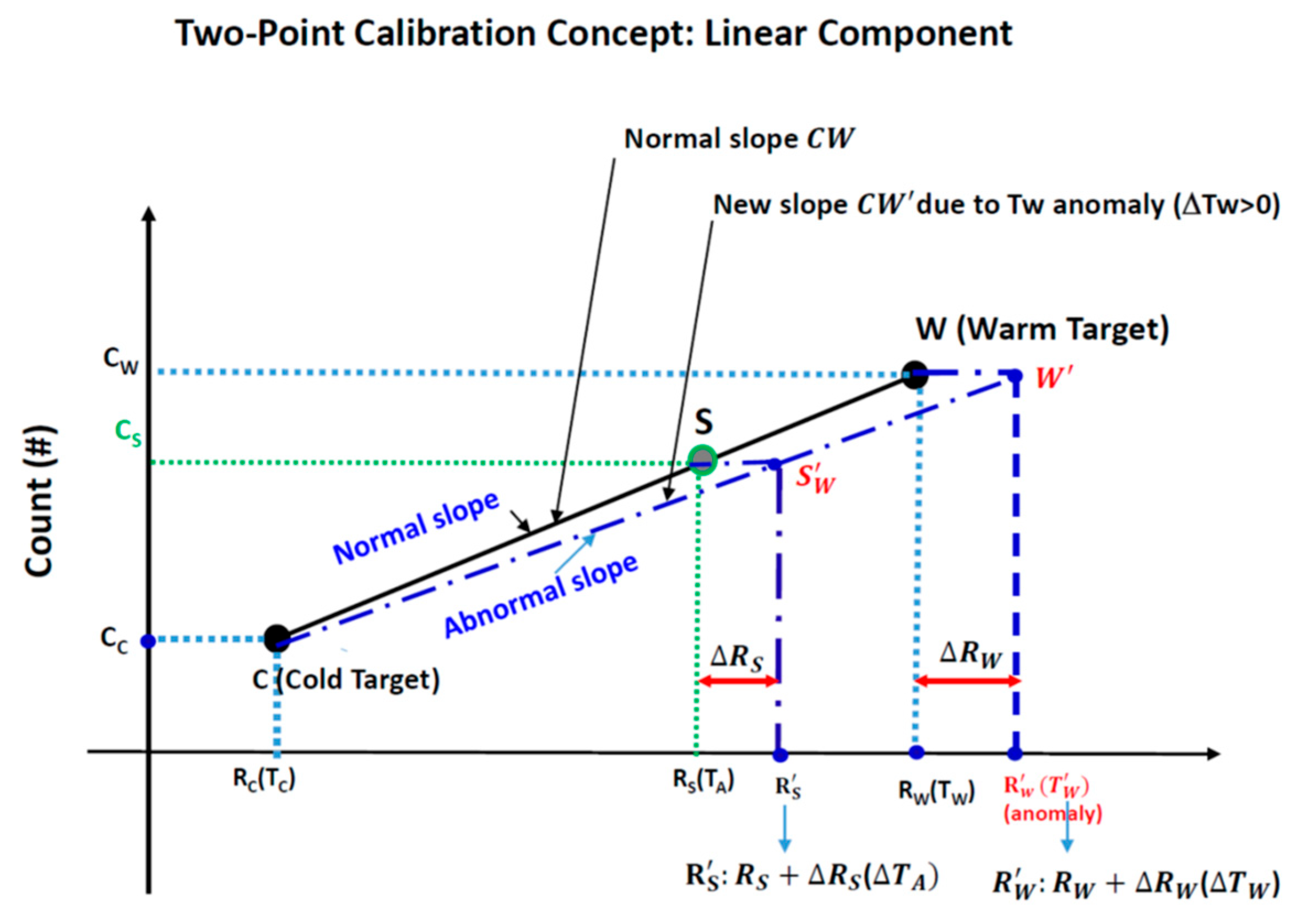
4. Implication for Calibration Radiometric Accuracy
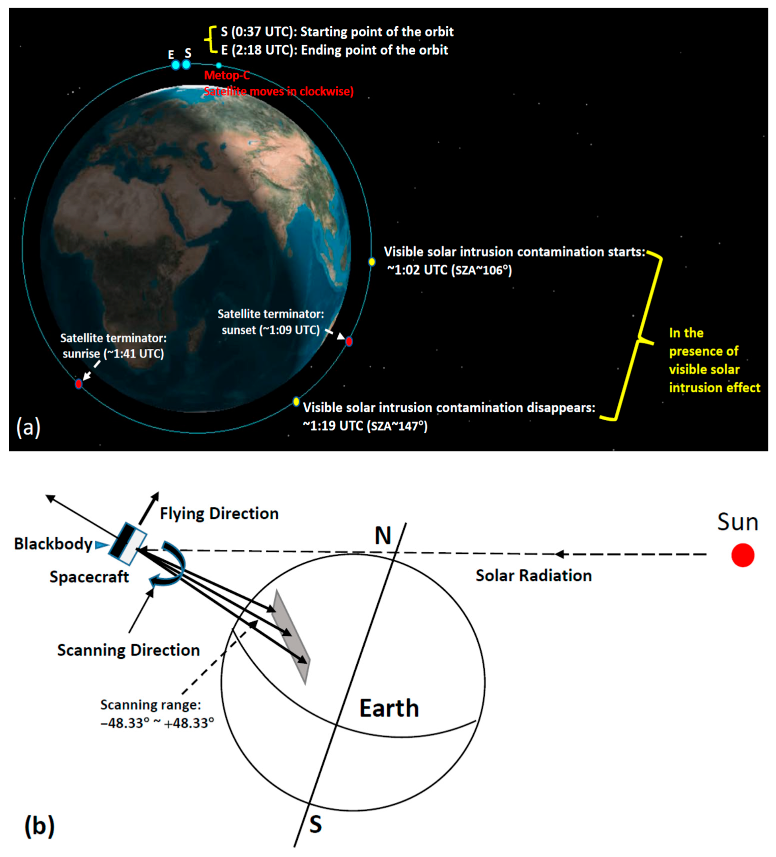
5. Root Cause Analysis of the Anomalous Pattern Problem
6. Summary and Conclusions
Author Contributions
Funding
Data Availability Statement
Acknowledgments
Conflicts of Interest
Disclaimer
References
- Northrop Grumman Electronic Systems (NGES). AMSU-A System Operation and Maintenance Manual for METSAT/METOP, S/N 105 through 109; Technique Report NAS 5-32314 CDRL 307; NGES: Linthicum Heights, MD, USA, 2010. [Google Scholar]
- Northrop Grumman Electronic Systems (NGES). Calibration Log Book for the Advanced Microwave Sounding Unit-A (AMSU-A); Report #10481A; Aerojet: Azusa, CA, USA, 1995. [Google Scholar]
- Northrop Grumman Electronic Systems (NGES). Calibration Log Book for AMSU-A2 SN 107; Report No. 15267; Northrop G Grumman: Azusa, CA, USA, 2008; p. 91702. [Google Scholar]
- Mo, T.; Weinreb, M.; Grody, N.; Wark, D. AMSU-A Engineering Model Calibration; NOAA Technical Report NESDIS 68; NOAA: Silver Spring, MD, USA, 1993. [Google Scholar]
- Mo, T. Prelaunch calibration of the Advanced Microwave Sounding Unit-A for NOAA-K. IEEE Trans. Microw. Theory Technol. 1996, 44, 1460–1469. [Google Scholar] [CrossRef]
- Mo, T. AMSU-A Antenna Pattern Corrections. IEEE Trans. Geosci. Remote Sens. 1999, 37, 103–112. [Google Scholar]
- Mo, T. Calibration of the Advanced Microwave Sounding Unit-A Radiometer for MetOp-A; NOAA Technical Report NESDIS 121; United States Department of Commerce: Washington, DC, USA, 2006. [Google Scholar]
- Mo, T.; Kigawa, S. A study of lunar contamination and onorbit performance of the NOAA-18 Advanced Microwave Sounding Unit-A. J. Geophys. Res. 2007, 112, D20124. [Google Scholar] [CrossRef]
- Mo, T. Postlaunch calibration of the MetOp-A Advanced Microwave Sounding Unit-A. IEEE Trans. Geosci. Remote Sens. 2008, 46, 3581–3600. [Google Scholar] [CrossRef]
- Tian, M.; Zou, X.; Weng, F. Use of Allan Deviation for Characterizing Satellite Microwave Sounder Noise Equivalent Differential Temperature (NEDT). IEEE Geosci. Remote Sens. Lett. 2015, 12, 2477–2480. [Google Scholar] [CrossRef]
- Yan, B.; Wu, X.; Chen, J.; Ahmad, K.; Kireev, S.; Qian, H.; Zou, C.-Z.; Cao, C. Metop-C AMSU-A and AVHRR Sensor Data Recorder (SDR) Data Calibration/Validation (CalVal): Status & Prospective. In Proceedings of the 2019 Conference on Characterization and Radiometric Calibration for Remote Sensing, Logan, UT, USA, 21–24 August 2019; Available online: https://digitalcommons.usu.edu/cgi/viewcontent.cgi?article=1358&context=calcon (accessed on 1 September 2019).
- Yan, B.; Chen, J.; Zou, C.-Z.; Ahmad, K.; Qian, H.; Garrett, K.; Zhu, T.; Han, D.; Green, J. Calibration and Validation of Antenna and Brightness Temperatures from Metop-C Advanced Microwave Sounding Unit-A (AMSU-A). Remote Sens. 2020, 12, 2978. [Google Scholar] [CrossRef]
- Yan, B.; Ahmad, K. Derivation and Validation of Sensor Brightness Temperatures for Advanced Microwave Sounding Unit-A Instruments. IEEE Trans. Geosci. Remote Sens. 2020, 59, 404–414. [Google Scholar] [CrossRef]
- Yan, B.; Kireev, S.V. A New Methodology on Noise Equivalent Differential Temperature Calculation for On-Orbit Advanced Microwave Sounding Unit—A Instrument. IEEE Trans. Geosci. Remote Sens. 2021, 59, 8554–8567. [Google Scholar] [CrossRef]
- Derber, J.C.; Wu, W.S. The use of TOVS cloud-cleared radiances in the NCEP SSI analysis system. Mon. Weather Rev. 1998, 126, 2287–2299. [Google Scholar] [CrossRef]
- Zhu, T.; Zhang, D.-L.; Weng, F. Impact of the Advanced Microwave Sounding Unit Measurements on Hurricane Prediction. Mon. Weather. Rev. 2002, 130, 2416–2432. [Google Scholar] [CrossRef]
- Kelly, G.; Thépaut, J.-N. Evaluation of the Impact of the Space Component of the Global Observation System through Observing System Experiments; ECMWF Newsletter, No. 113; ECMWF: Reading, UK, 2007; pp. 16–28. Available online: https://www.ecmwf.int/sites/default/files/elibrary/2007/17527-evaluation-impact-space-component-global-observing-system-through-observing-system-experiments.pdf (accessed on 1 December 2007).
- Zou, X.L.; Qin, Z.; Weng, F. Impacts from assimilation of one data stream of AMSU-A and MHS radiances on quantitative precipitation forecasts. Q. J. R. Meteorol. Soc. 2017, 143, 731–743. [Google Scholar] [CrossRef]
- Weng, F.; Zhao, L.; Ferraro, R.R.; Poe, G.; Li, X.; Grody, N.C. Advanced microwave sounding unit cloud and precipitation algorithms. Radio Sci. 2003, 38, 8086–8096. [Google Scholar] [CrossRef]
- Zhu, T.; Weng, F. Hurricane Sandy warm-core structure observed from advanced Technology Microwave Sounder. Geophys. Res. Lett. 2013, 40, 3325–3330. [Google Scholar] [CrossRef]
- Tian, X.; Zou, X. ATMS- and AMSU-A-derived hurricane warm core structures using a modified retrieval algorithm. J. Geophys. Res. Atmos. 2016, 121, 12630–12646. [Google Scholar] [CrossRef]
- Zou, X.L. Climate trend detection and its sensitivity to measurement precision. Adv. Meteorol. Sci. Technol. 2012, 2, 41–43. [Google Scholar]
- Zou, C.Z.; Wang, W. Intersatellite calibration of AMSU-A observations for weather and climate applications. J. Geophys. Res. Atmos. 2011, 116, D23113. [Google Scholar] [CrossRef]
- Zou, C.Z.; Wang, W.; NOAA CDR Program. NOAA Fundamental Climate Data Record (FCDR) of AMSU-A Level 1c Brightness Temperature, Version 1.0.; NOAA National Climatic Data Center: Silver Spring, MD, USA, 2013. [CrossRef]
- Twarog, E.M.; Purdy, W.E.; Gaiser, P.W.; Cheung, K.H.; Kelm, B.E. WindSat on-orbit warm load calibration. IEEE Trans. Geosci. Remote Sens. 2006, 44, 516–529. [Google Scholar] [CrossRef]
- Wentz, F.; Gentemann, C.L.; Ashcroft, P.D. On-Orbit Calibration of AMSR-E and the Retrieval of Ocean Products. In Proceedings of the 83rd AMS Annual Meeting, Long Beach, CA, USA, 9–13 February 2003; Paper P5.9. Available online: http://images.remss.com/papers/rssconf/wentz_ams_2003_longbeach_amsre_calibration.pdf (accessed on 1 October 2003).
- Meissner, T.; Wentz, F. Intercalibration of AMSR-E and WindSat brightness temperature measurements over land scenes. In Proceedings of the 2010 IEEE International Geoscience and Remote Sensing Symposium, Honolulu, HI, USA, 25–30 July 2010; pp. 3218–3219. [Google Scholar] [CrossRef]
- Cao, C.; Weinreb, M.; Sullivan, J. Solar contamination effects on the infrared channels of the advanced very high resolution radiometer (AVHRR). J. Geophys. Res. 2001, 106, 33463–33469. [Google Scholar] [CrossRef]
- Walton, C.; Sullivan, J.T.; Rao, C.R.N.; Weinreb, M.P. Corrections for detector nonlinearities and calibration inconsistencies of the infrared channels of the advanced very high-resolution radiometer. J. Geophys. Res. 1998, 103, 3323–3337. [Google Scholar] [CrossRef]
- Weng, F.; Zou, X.; Sun, N.; Yang, H.; Tian, M.; Blackwell, W.J.; Wang, X.; Lin, L.; Anderson, K. Calibration of Suomi national polar-orbiting partnership advanced technology microwave sounder. J. Geophys. Res. 2013, 118, 11,187–11,200. [Google Scholar] [CrossRef]
- Jeffrey, R.; Graumann, A. NOAA KLM USER’S GUIDE with NOAA-N, N Prime, and MetOp SUPPLEMENTS (1-2530); National Oceanic and Atmospheric Administration, National Environmental Satellite, Data, and Information Service, National Climatic Data Center: Asheville, NC, USA, 2014. [Google Scholar]
- Weng, F.; Zou, X. Errors from Rayleigh–Jeans approximation in satellite microwave radiometer calibration systems. Appl. Opt. 2013, 52, 505–508. [Google Scholar] [CrossRef] [PubMed]
- Zou, C.; Qian, H. Prelaunch Calibration of the Advanced Microwave Sounding Unit-A Radiometer for MetOp-C; NOAA/STAR Technical Report; United States Department of Commerce: Washington, DC, USA, 2018. [Google Scholar]
- Bell, S.A. Beginner’s Guide to Uncertainty of Measurement; National Physical Laboratory: Middlesex, UK, 1999; Issue 2; p. 33. [Google Scholar]
- Zou, C.-Z.; Xu, H.; Hao, X.; Fu, Q. Post-millennium atmospheric temperature trends observed from satellites in stable orbits. Geophys. Res. Lett. 2021, 48, e2021GL093291. [Google Scholar] [CrossRef]
- Hans, I.; Burgdorf, M.; John, V.O.; Mittaz, J.; Buehler, S.A. Noise performance of microwave humidity sounders over their life Time. Atmos. Meas. Tech. 2017, 10, 4927–4945. [Google Scholar] [CrossRef]
- Yang, J.X.; Yang, H. A new algorithm for determining the noise equivalent delta temperature of in-orbit microwave radiometers. IEEE Trans. Geosci. Remote. Sens. 2021, 60, 1–11. [Google Scholar] [CrossRef]
- Vallado, D.; Crawford, P.; Hujsak, R.; Kelso, T. Revisiting Spacetrack Report #3. In Proceedings of the Astrodynamics Specialist Conference, Keystone, CO, USA, 21–24 August 2006; American Institute of Aeronautics and Astronautics: Reston, VA, USA, 2006; ISBN 978-1-62410-048-2. [Google Scholar] [CrossRef]
- Cao, C.; Weinreb, M.; Xu, H. Predicting Simultaneous Nadir Overpasses among Polar-Orbiting Meteorological Satellites for the Intersatellite Calibration of Radiometers. J. Atmos. Ocean. Technol. 2004, 21, 537–542. [Google Scholar] [CrossRef]
- Joint Polar Satellite System (JPSS). Advanced Technology Microwave Sounder (ATMS) SDR Calibration Algorithm Theoretical Basis Document (ATBD); Center for Satellite Applications and Research: College Park, MD, USA, 2013. Available online: https://www.star.nesdis.noaa.gov/jpss/documents/ATBD/D0001-M01-S01-001_JPSS_ATBD_ATMS-SDR_B.pdf (accessed on 30 December 2022).


| Ch. | Center Frequency (MHz) | Conversion Bandwidth (MHz) | Temperature Sensitivity NEDT (K) |
|---|---|---|---|
| 1 | 23,800 | 270 | 0.3 |
| 2 | 31,400 | 180 | 0.3 |
| 3 | 50,300 | 180 | 0.4 |
| 4 | 52,800 | 400 | 0.25 |
| 5 | 53,596 ± 115 | 170 | 0.25 |
| 6 | 54,400 | 400 | 0.25 |
| 7 | 54,940 | 400 | 0.25 |
| 8 | 55,500 | 330 | 0.25 |
| 9 | fo = 57,290.344 | 330 | 0.25 |
| 10 | fo ± 217 | 78 | 0.4 |
| 11 | fo ± 322.2 ± 48 | 36 | 0.4 |
| 12 | fo ± 322.2 ± 22 | 16 | 0.6 |
| 13 | fo ± 322.2 ± 10 | 8 | 0.8 |
| 14 | fo ± 322.2 ± 4.5 | 3 | 1.2 |
| 15 | 89,000 | 1500 | 0.5 |
| Symbol | Quantity |
|---|---|
| by using the inverse of Planck function | |
| Kinetic or bulk temperature of the blackbody target (warm load), also named as warm load PRT temperature | |
| Cosmic temperature after certain corrections [12] | |
| using Planck function | |
| using Planck function | |
| Warm load radiometric count (warm count), corresponding to the radiative temperature of the blackbody target | |
| Cold space radiometric count (cold count) | |
| Earth scene radiometric count (scene count) | |
| Q | Nonlinearity of instrument square-law detector in radiance domain |
| Nonlinearity in temperature domain | |
| μ | Nonlinearity parameter μ in radiance domain |
| Nonlinearity parameter μ in temperature domain | |
| Calibration channel gain in the domain of radiance | |
| Calibration channel gain in the domain of temperature |
| Channel Index | Error (K) | Error (K) | Error (K) | |||
|---|---|---|---|---|---|---|
| 1 | 0.22 | 0.09 | 0.05 | 0.01 | 0.16 | 0.05 |
| 2 | 0.19 | 0.06 | 0.05 | 0.01 | 0.17 | 0.05 |
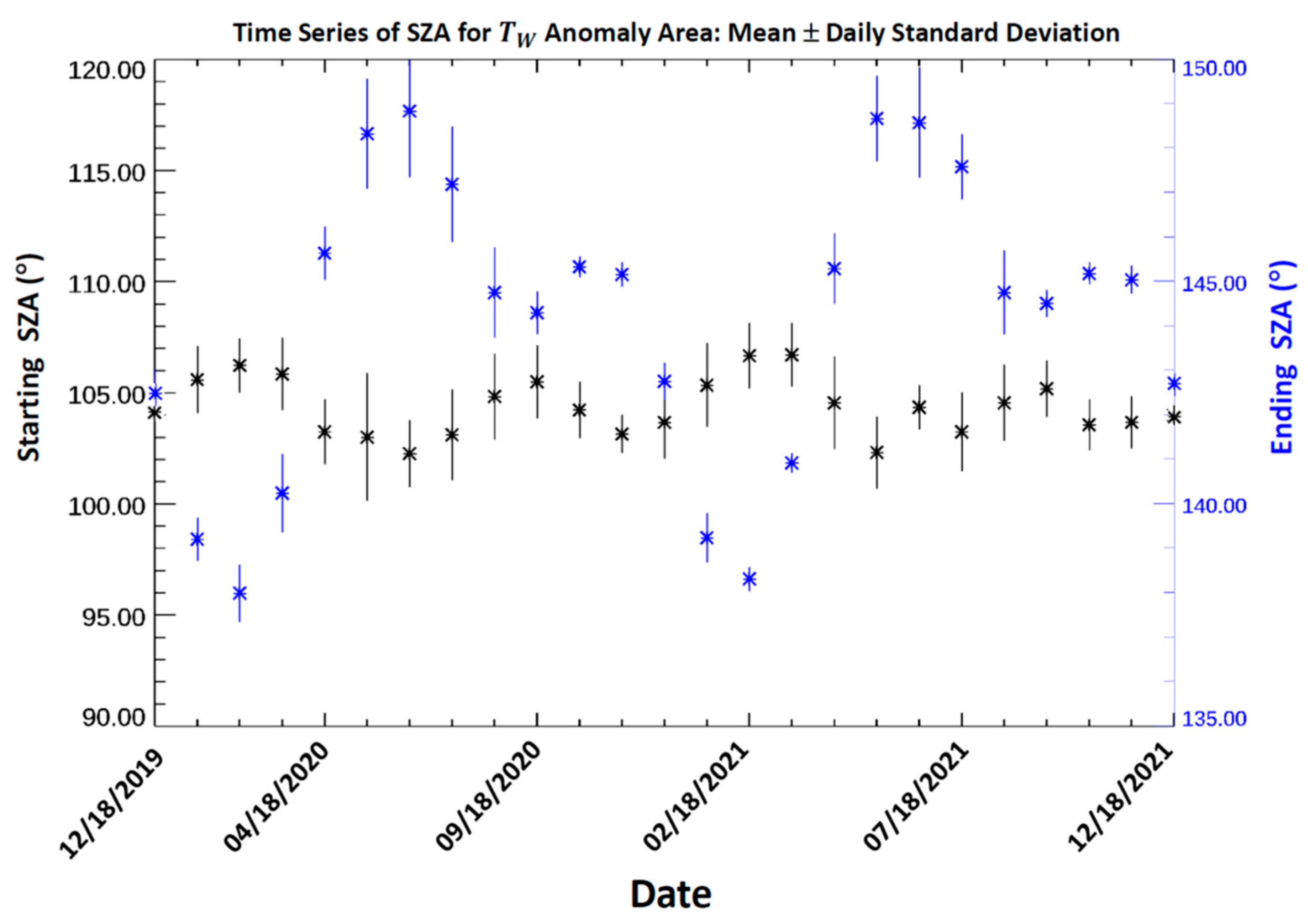
| Starting SZA (°) | Ending SZA (°) | ||
|---|---|---|---|
| 104.35 | 1.53 | 144.12 | 0.67 |
Disclaimer/Publisher’s Note: The statements, opinions and data contained in all publications are solely those of the individual author(s) and contributor(s) and not of MDPI and/or the editor(s). MDPI and/or the editor(s) disclaim responsibility for any injury to people or property resulting from any ideas, methods, instructions or products referred to in the content. |
© 2024 by the authors. Licensee MDPI, Basel, Switzerland. This article is an open access article distributed under the terms and conditions of the Creative Commons Attribution (CC BY) license (https://creativecommons.org/licenses/by/4.0/).
Share and Cite
Yan, B.; Cao, C.; Sun, N. Effects of Solar Intrusion on the Calibration of the Metop-C Advanced Microwave Sounding Unit-A2 Channels. Remote Sens. 2024, 16, 864. https://doi.org/10.3390/rs16050864
Yan B, Cao C, Sun N. Effects of Solar Intrusion on the Calibration of the Metop-C Advanced Microwave Sounding Unit-A2 Channels. Remote Sensing. 2024; 16(5):864. https://doi.org/10.3390/rs16050864
Chicago/Turabian StyleYan, Banghua, Changyong Cao, and Ninghai Sun. 2024. "Effects of Solar Intrusion on the Calibration of the Metop-C Advanced Microwave Sounding Unit-A2 Channels" Remote Sensing 16, no. 5: 864. https://doi.org/10.3390/rs16050864
APA StyleYan, B., Cao, C., & Sun, N. (2024). Effects of Solar Intrusion on the Calibration of the Metop-C Advanced Microwave Sounding Unit-A2 Channels. Remote Sensing, 16(5), 864. https://doi.org/10.3390/rs16050864