Abstract
Automated built-up infrastructure classification is a global need for planning. However, individual indices have weaknesses, including spectral confusion with bare ground, and computational requirements for deep learning are intensive. We present a computationally lightweight method to classify built-up infrastructure. We use an ensemble of spectral indices and a novel red-band texture layer with global thresholds determined from 12 diverse sites (two seasonally varied images per site). Multiple spectral indexes were evaluated using Sentinel-2 imagery. Our texture metric uses the red band to separate built-up infrastructure from spectrally similar bare ground. Our evaluation produced global thresholds by evaluating ground truth points against a range of site-specific optimal index thresholds across the 24 images. These were used to classify an ensemble, and then spectral indexes, texture, and stratified random sampling guided training data selection. The training data fit a random forest classifier to create final binary maps. Validation found an average overall accuracy of 79.95% (±4%) and an F1 score of 0.5304 (±0.07). The inclusion of the texture metric improved overall accuracy by 14–21%. A comparison to site-specific thresholds and a deep learning-derived layer is provided. This automated built-up infrastructure mapping framework requires only public imagery to support time-sensitive land management workflows.
1. Introduction
Accurate and timely detection and mapping of built-up infrastructure is critical for monitoring population dynamics, urban planning, natural habitat loss, disaster response, mobility mapping, and much more [1]. However, this land cover class requires robust and flexible methods of detection. Built-up infrastructure includes buildings, roads, and other artificial structures. These consist of a wide range of materials with different spectral signatures, such as concrete, asphalt, steel, ceramic, and others [2]. Built-up infrastructure and bare-ground areas may have similar density and composition, resulting in broad spectral overlap and similar spectral reflectance, causing frequent misclassification [3,4].
Worldwide built-up infrastructure land cover is expected to double between 2000 and 2050, increasing particularly rapidly across densely populated areas such as megacities including Tokyo, Delhi, and Shanghai and the Pearl River Delta and Jakarta metropolitan regions [5]. While built-up infrastructure is currently estimated to occupy only about 0.6% of the land surface, the impacts on the environment are wide-reaching [6]. For example, built-up infrastructure in dense urban environments has led to urban heat island effects and, consequently, severe public health episodes in many countries [7,8]. Concentrated areas of built-up infrastructure often suffer from high air pollution and degraded air quality, with urban air pollution and heat effects linked to millions of premature deaths globally [9,10,11,12]. Urban areas associated with built-up infrastructure have been linked to unsustainable resource extraction [13]. Moreover, many already-developed megacities have experienced ongoing land use intensification (e.g., higher-density buildings) as well as extensification (e.g., urban sprawl) [14].
Considering the rapid expansion, importance, and impact of built-up infrastructure, many previous studies created techniques to address the need to map this phenomenon to support monitoring, planning, and policy [1]. Many early efforts to map built-up infrastructure relied on manual delineation of imagery [15,16]. Later efforts included manual collection of training data for use in a classification algorithm with various types of satellite or airborne imagery [17]. For example, a study using ASTER imagery over Indiana, USA achieved promising results using the self-organizing map and multi-layer perceptron methods [18]. In more recent years, studies have leveraged C-band, X-band, or L-band SAR time series [19,20,21] or VIIRS Nighttime lights time series with promising results [22,23]. Recent studies have also leveraged machine or deep learning with manual training data or use of existing training data such as OpenStreetMap with accuracies exceeding 90% [24,25,26,27].
Different methods offer accuracy tradeoffs with the cost of manual input, data acquisition and availability, and computational intensity. Although manual delineation or manually set thresholds can be used instead of automated processes to mitigate spectral confusion, doing so is time-consuming and reduces the utility of data for near-real-time applications. While some studies apply ancillary datasets that support highly accurate built-up area mapping [28,29,30], these efforts can be data-intensive and time-consuming for certain applications, and relevant ancillary datasets may not exist for all areas of interest. Further, studies have accurately leveraged time series of imagery for built-up area mapping [19,31,32], but, these methods tend to be computationally or data-intensive and require collecting a time series of imagery. Single-date analysis offers faster results with less data intensity.
Many spectral indices were created to address the need for built-up infrastructure mapping from publicly available multispectral data with global coverage and frequent revisits. Combining multiple indices can reduce the effect of index bias. However, many indices have similar types of problematic misclassification, predominantly consisting of erroneous commission of bare ground [33,34,35,36,37,38]. For example, an early commonly cited index, the Normalized Difference Built-up Index (NDBI) by Zha et al. [38], used a ratio of shortwave infrared (SWIR) and near-infrared (NIR) bands to differentiate built-up land cover and expedite mapping. In this study, results were comparable to manual and maximum likelihood methods when applied to a study area in eastern China, but displayed confusion between barren land, beaches, and areas affected by drought. Bouzekri et al. [33] developed improvements using their Built-up Area Extraction Index (BAEI) to combine the red, green, and SWIR bands from the Landsat Operational Land Imager and Thermal Infrared Sensor (OLI-TIRS) to classify built-up infrastructure over North Algeria. The visible blue band and first shortwave infrared index (VBI-sh) introduced by Ezimand et al. [34] is a normalized index that uses a blue and SWIR band and outperformed six compared indices over a study site in Iran. The Band Ratio for Built-up Area (BRBA) was developed by Waqar et al. [36] to use red (0.63–0.69 µm) and SWIR (1.55–1.75 µm) bands with additional contrast stretching over their study site in Pakistan. Firozjaei et al. [35] introduced the Automated Built-up Extraction Index (ABEI), which adjusted seven bands using coefficients determined using IGSA optimization and was tested over 16 cities in Europe and 5 locations in Iran. Our study uses an ensemble of indices to strengthen model decision-making and avoid weaknesses of individual indices.
Texture analysis has been used as a direct or supplemental method for built-up cover classification for decades. There are many categories of approach, including statistical analysis of single spectral bands, such as that described in this study. Haralick et al. [39] provided application of statistical methods, including calculation of variance and deviation to land cover classification of photomicrographs, aerial photography, and multispectral satellite imagery, with respective accuracies of 89, 82.3, and 83.5%. Weszka [40] also examined several approaches, including statistical analysis, and found calculating the means of neighborhood groupings to be useful. Irons and Petersen [41] calculated variance in a 3 × 3-pixel window as well as other statistics for four Landsat bands, finding texture transformations ineffective for land cover classification at the coarse spatial resolution studied (79 × 57 m).
The addition of edge detection or contrast enhancement is increasingly included in recent literature workflows to improve accuracy. Ezimand et al. [34] investigated the benefits of including histogram equalization, which increases contrast by balancing the number of pixels between shades of gray. Chen et al. [42] found a high-pass filter for edge enhancement additionally useful alongside histogram equalization when mapping infrastructure for change detection. In a comparative study of 12 algorithms for rapid mapping of land cover over three global sites, a high-pass filter method performed consistently well [43]. Pesaresi et al. [44] used GCLM-derived measures on 5 m resolution panchromatic imagery over three dates over a single site to achieve an average overall accuracy (OA) of 86.7%, with an average commission error of 25.8%. Brahme et al. [3] found that incorporating eight GLCM-based textural features increased accuracy by 4.91%.
Our texture metric uses a 3 × 3 window with a single statistical metric on a single enhanced red band. This computationally lightweight method uses the commonly collected red bandwidth to distinguish between rough built-up cover and smoother bare ground. This combines edge enhancement and local statistical deviation to address the common weakness of bare-ground commission error.
Our workflow also incorporates masking of the ensemble and training data to improve model inputs. Spectral indices targeting other land covers are often used in literature studies to directly mask water or vegetation or indirectly influence the index formula [23,36,37]. The Index-based Built-up Index (IBI) introduced by Xu et al. [37] enhanced NDBI in their study over southeastern China by combining it with a Soil Adjusted Vegetation Index (SAVI) and the modified normalized difference water index (MNDWI). The IBI sought to control spectral confusion by using combined indices rather than original bands to reduce dimensionality and redundancy. Similarly, Xu et al. [45] arranged the Normalized Difference Impervious Surface Index (NDISI) to leverage either NDWI or MNDWI within its formula, which was retained in derivative indices Modified Normalized Difference Impervious Surface Index (MNDISI) and the Enhanced Normalized Difference Impervious Surfaces Index (ENDISI) [46,47]. Conclusions in Waqar et al. [36] emphasized the utility of water masking. Zha et al. [38] subtract NDVI values from NDBI values to assist in recoding values, and Bouzekri et al. [33] note that misclassification in their index would improve by masking vegetation prior to applying the BAEI index. Given the successful use of masking in literature, our workflow incorporates both a water and vegetation mask.
Previous work showed the advantages of using machine learning models (e.g., random forest) trained on automatically selected data over randomly selected training data from spectral index ensembles for other land cover types [48]. This study incorporates machine learning similarly for final binary classification, using an ensemble of masked spectral indices to create and refine training data for a random forest classifier. Random forest was chosen due to its strong performance as a classifier in various land cover classification applications [49,50]. In a similar previous study by Lasko et al. [48], RF slightly outperformed gradient-boosted trees (GBT), performed more consistently than support vector machine (SVM) over different resolutions, and had a shorter runtime and reduced computational requirements compared to a majority vote classifier (which combined random forest, GBM, and SVM results). Other studies with fewer sites and images found slight or moderate advantages in other models, including newer models such as lightGBM and XGBoost. McCarty et al. [51] found similar OA results between RF (0.594), SVM (0.642), and lightGBM (0.653) when performing land cover classification over a single site. Abdi [52] found similar OA results across four dates over one site when comparing SVM (0.758), extreme gradient boosting (0.751), RF (0.739), and deep learning (0.733). Ramdani and Furqon [53] found better RMSE values when using XGBoost than Artificial Neural Network (ANN), RF, and SVM (respectively 1.56, 4.33, 6.81, and 7.45) when classifying urban forest at a single site. Georganos et al. [54] found that Xgboost, when parameterized with a Bayesian procedure, systematically outperformed RF and SVM, mainly with larger sizes of training data, over three sites. RF was selected for this study due to the large body of literature supporting it as a consistently robust, stable, and efficient option across a wide range of sites. However, new-generation boosting algorithms are becoming more efficient, and while out of scope for this study, future work may benefit from exploring them.
Deep learning methods may improve accuracy but are computationally intensive. The comparatively greater infrastructure and time requirements may be prohibitive for some time-sensitive applications. Our study details comparative improvement between the deep learning derived Global Human Settlement (GHS) layer and our RF workflow output made with reduced computational requirements [44,55]. The GHS layer was created using deep learning convolutional neural networks (CNNs) on high-performance computational equipment [55]. A 2019 meta-analysis found studies of land use/land cover (LULC) classification achieved high levels of accuracy when using deep learning [56]. However, many of these studies used hyperspectral or very high-resolution imagery, which may limit application, as these data are not yet publicly globally available. The GHS, however, used Sentinel-2 imagery, as does this study, and showed improved accuracy. Conversely, other studies have found limited gain. Jozdani et al. [57] compared deep learning methods, including convolutional neural network (CNN), multilayer perceptron (MLP), regular autoencoder (RAE), sparse autoencoder (SAE), and variational autoencoder (AE) methods to common machine learning methods, such as RF, SVM, GBT, and XGBoost. Jozdani et al. [57] found all methods resulted in F1 values within 0.029 or less from one another and OA values within 2.86% or less from one another. These findings suggest that the intense computational requirements of deep learning may not justify the small gain in accuracy for all use cases and support other findings that many ML methods yield similar accuracy, though performance varies by scene.
Consistent challenges to global built-up mapping have included resource requirements in the form of manual threshold choice, manual creation of training data, creation of time series, availability of ancillary data, and prohibitive computational infrastructure requirements. The objective of this study is to address a balance of these. We provide a robust automatic classification of built-up pixels across a wide variety of sites using a computationally light machine learning workflow. It requires minimal manual user input by providing default thresholds and automating training data selection. It uses a single date image without ancillary data. Texture is used additionally to address the common misclassification of bare ground. As shown in the studies above, many methods to automate built-up land cover extraction, but few test more than two regional study sites, and misclassification with bare ground remains a consistent concern. We present a method with utility over a variety of internationally distributed sites that display a wide range of construction types and built-up land cover patterns. We achieve this by using single-date Sentinel-2 10 m imagery without ancillary datasets or tedious manual training collection, which enhances the ability for rapid, regional-scale mapping as compared with time series methods or those reliant on multisource data fusion. This effort evaluates globally optimal thresholds, which are determined using the 24 seasonally opposed images across 12 international sites. A novel red-band texture metric is created and evaluated for its ability to reduce the main cause of error, false-positive built-up pixels, in the workflow.
2. Materials and Methods
2.1. Data: Sentinel-2 Imagery and Global Human Settlement Layer
Sentinel-2 (S2) Level 2A (L2A) Bottom of Atmosphere (BoA) reflectance imagery was collected from the Copernicus Open Access Hub, where it is provided to the public by the European Space Agency. S2 included the five bands (Table 1) that supported the calculation of five built-up spectral indices, a texture layer, and two masks in this study. The four shorter wavelength VIS-NIR bands were provided at 10 m resolution. The SWIR band was provided at 20 m resolution and was resampled to 10 m with the nearest neighbor method.

Table 1.
The bands used in this workflow were subset from Sentinel-2 multispectral imagery. Visible and Near-Infrared (VNIR) bands were provided at 10 m. The SWIR band was provided at 20 m and resampled to 10 m for processing.
The GHS layer was used here to compare the accuracy of output from a deep learning method to that of our workflow. Sentinel-2 imagery used for the GHS was filtered using a best-available-pixel method on Google Earth Engine, which creates composite images from pixels with low cloud scores [55,58]. The GHS is a multi-model method based on a CNN framework [55]. It included 485 models trained on 615 Universal Transverse Mercator grid zones [55]. The 15 TB input data were hosted on and processed by the Joint Research Centre (JEODPP) using two GPU nodes that trained and predicted classifications, with an average runtime of roughly 6 h per UTM grid zone [55]. The global classification layer was downloaded from the European Commission’s Joint Research Centre website [44].
2.2. Study Sites
Sites were selected based on three variables: Human Development Index (HDI), infrastructure density, and geographic features of interest, with the primary objective of selecting varied and difficult sites to map built-up areas (Figure 1). First, to capture differences in wealth that may influence variation in building materials and construction methods and consequentially variation in resulting spectral patterns, researchers used the Human Development Index (HDI) to select regions with a representative distribution of development rankings (Table 2) [59]. The HDI is an index derived from a nation’s longevity, educational system, and income and is used to compare certain aspects of human development [59].
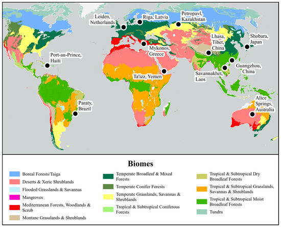
Figure 1.
Twelve study sites were selected worldwide to capture variations in development and infrastructure density. Sentinel-2 L2A imagery was collected for two dates at each site, resulting in 24 scenes.
Table 2.
The twelve study site locations are listed with their Sentinel-2 Granule ID, Human Development Index ranking [59], the estimated infrastructure density development in the scene, and characterizing features that may differ between scenes. The date with comparatively greater natural vegetation in each site pair was considered the “leaf-on” date and is marked with an asterisk.
Second, to capture built-up infrastructure patterns associated with different population densities, researchers then considered scenes that contained predominantly high-, medium-, or low-density development (Table 2). Four scenes of each density level were chosen.
Third, scenes were chosen through additional exploratory review to add complexity and difficulty in spectral classification. This includes areas with aquaculture and wetlands (such as Savannahket), large swathes of bare ground that were either visually similar (Ta’izz) or dissimilar to building materials (Alice Springs), many sites with coastline (Mykonos), mountains (Lhasa), and areas with high variation in built-up infrastructure (Guangzhao). Selected areas contained a variety of nontarget land covers, by intent, that may confuse the built-up infrastructure classification, such as high- and low-contrast bare ground, including fallow agriculture and beaches; sparse to thick vegetation, including dryland, grassland, and forest; water bodies, including ocean, lakes, rivers, wetland, and aquaculture; and snow. These areas were chosen through exploratory review rather than random sampling because these features may either be relatively rare or small in area, and it is difficult to ensure their representation in a random selection or difficult to define in classification, which makes them difficult to sample automatically from existing data. Ten of the fourteen major biomes defined by Dinerstein et al. [60] are represented within these sites, primarily excluding high-latitude biomes and temperate conifer forest. The ten biomes represented in this sample cover 76.2% of terrestrial area (Table 3) [60]. While individual scenes contain localized complexity, this offers a general variation of nontarget terrestrial natural vegetation as context.
Table 3.
Fourteen biomes are shown with ID numbers and percent of terrestrial area covered, as created and calculated by Dinerstein et al. [60], alongside the number of sites they overlap in this study. Biomes were delineated to assess overlap using the 2017 RESOLVE Ecoregions dataset [60].
Researchers chose scenes collected between the years 2020 and 2021. Cloud presence was avoided when possible. Scenes were chosen as close to 6 months apart as possible to capture regional seasonal variation, such as agricultural and aquacultural changes, as well as natural vegetation senescence. The sites are listed in Table 2 along with their Sentinel-2 granule identifier, collection date, and characterization.
2.3. Software and Programs
Our workflow was created in Python 3.6.7 using functions from the ArcPy Spatial Analyst and Management libraries and GDAL. These functions were used to:
- calculate spectral indices and the texture layer;
- exclude clouds and saturated pixels;
- mask vegetation and water;
- select balanced random sampling for ground truthing and separately for training data;
- label training data;
- apply an RF machine learning classifier; and
- batch calculate validation statistics.
Thresholds and subset selections were applied using “Reclassify”. Images were masked using “Extract By Mask”. The texture layer used “Filter” on a “High Pass” setting, “Block Statistics” to find the standard deviation within a 3 × 3-pixel window, and “Slice” was used to apply Natural Breaks clustering. More detail on the purpose and application of the texture layer creation is discussed in Section 2.7. The training data were automatically selected from the ensemble using “Create Accuracy Assessment Points” and using an equalized stratified random distribution and were assigned values using “Extract MultiValues To Points” and cleaned using “Update Cursor”. To perform the supervised classification, “Composite Bands” assembled the reclassified ensemble of indices for input into “Train Random Trees Classifier”. The validation used “Create Accuracy Assessment Points” to select random stratified ground truth points, which were manually reviewed by researchers. Accuracy metrics were calculated using “Update Cursor” and the csv library. Visualizations were created in ArcGIS Pro, Version 3.0.3.
2.4. Methods Overview
In this study, we combine the advantages of different spectral indices in an ensemble to overcome potential misclassification biases of individual indices and then use the ensemble with a texture metric to train a machine learning classifier (Figure 2). Twelve diverse sites were selected to include built-up and nontarget land covers with varying conditions and with variation in target density, material, and construction type. We evaluated spectral index performance and thresholds for two seasonally opposed dates (winter and summer) per site to capture seasonal effects if applicable.
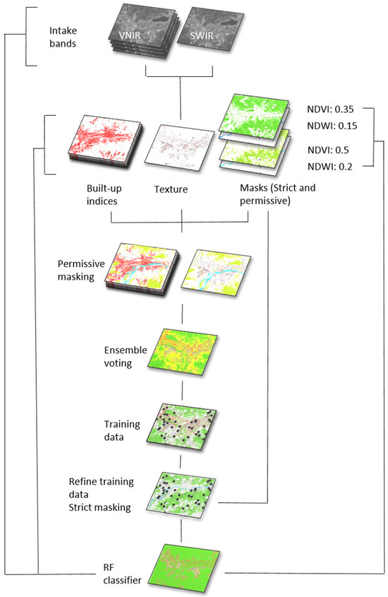
Figure 2.
Major steps in the methods are shown in this figure. Five VNIR/SWIR bands are used to calculate five built-up indices, a texture metric, and a permissive and a strict version of each water and vegetation mask. The built-up and texture layers are masked using the permissive NDVI and NWDI thresholds and then combined into an ensemble. Training data are taken from the low and high categories. Training data are then refined using the strict NDVI and NDWI, as well as the texture metric. It is input into the RF classifier along with the original VNIR/SWIR bands, built-up indices, texture, and strict masks to create a final binary classification.
Masking and use of filters, such as edge enhancement and increased contrast, were frequently cited in the literature as effective in improving classification results [36,37]. Early data exploration in our study found positive effects from such masking. Accordingly, we include water and vegetation indices in our workflow to first mask spectral indices after creation and then correct potentially confused training data labels (Figure 2).
To take advantage of edge enhancement and contrast, we created a novel texture raster from the red band using a high-pass filter and standard deviation of values within a pixel neighborhood (Figure 2). We use texture values to differentiate large areas of smooth bare ground, which have gradually transitioning values, from the spectrally similar built-up pixels, which often show sharper value transitions. We evaluated the performance of this metric for improving the overall accuracy of the model.
We tested a range of threshold options across all sites, and the highest-performing values were applied in the workflow as globally optimal defaults. These global thresholds were used to randomly select and label training data for a random forest (RF) machine learning classifier, thus automating the supervised classification to produce a binary map without time-consuming manual labeling (Figure 2). The use of multiple spectral indices reduced the biases of individual indices and strengthened the overall classification.
The workflow is hypothetically agnostic to any sensor that can provide the bands similar to those listed in Table 1. Due to the minimal input data requirements, provision of globally optimal thresholds, inclusion of texture index and masking, and ensemble-labeling of training data, this automated workflow avoids high processing-time costs while providing reasonable classification accuracy to support time-critical analysis needs for a land cover important to many decision-makers.
2.5. Spectral Index and Texture Metric Generation
The ensemble combined classified rasters of the following built-up infrastructure indices: NDBI, BAEI, VBI-sh, BRBA, an adjusted Index-based Built-up Index (IBI-adj), and Red Band High Pass Statistical Deviation (Texture). Indices were selected for classification performance and compatibility to shore up each other’s weaknesses and provide variation in the bands and combinations they rely on. In this study, the formula for IBI was adjusted to replace SAVI with NDVI and MNDWI with NDWI, as observed results between the substituted indices showed slight advantages in classification at the study sites and reusing similar masks would reduce overall computational load. Indices were calculated according to the formulas shown in Table 4.
Table 4.
Selected indices were calculated using the listed band combinations.
Our novel texture index differentiates between built-up infrastructure and spectrally similar bare ground through statistical deviation in the red band. Of the four 10 m VIS-NIR different bands tested, the red band contained high spectral separability between vegetation, built-up surface, and bare ground, as shown in Figure 3. To calculate the texture index, we first accentuated value differences in the red band using a high-pass filter with a 3 × 3-pixel neighborhood. We then took the standard deviation of the output, also using a 3 × 3-pixel window. Built-up land cover was observed to exhibit high standard deviation as compared with other land cover types. This index thus effectively captures the high spectral heterogeneity of built-up areas and allows us to exclude spectrally similar bare ground with lower heterogeneity.
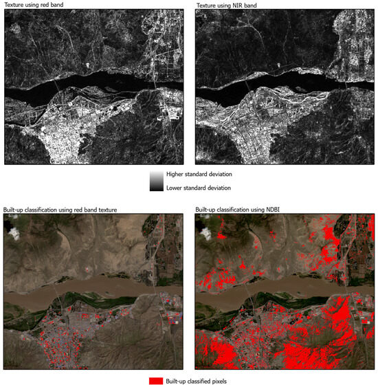
Figure 3.
Development and application of the texture layer is shown over a section of the Lhasa site. Texture calculated from the red and NIR bands is shown in the (top left) and (right). High standard deviation values are shown in white, representing “rougher” areas of high variation that tend to co-occur with infrastructure. Lower values are shown in darker gray, representing “smoother” areas that are more likely to be natural land covers that change gradually from pixel to pixel. Texture from the red band better separates vegetation and cloud from infrastructure. The red-band texture (bottom left) was applied in the workflow to select training data and mask nontarget bare ground, which is a common misclassification found in built-up indices, such as NDBI (bottom right).
2.6. Ground Truth Review of Scene-Specific Index Thresholds
To select ground truth points and calculate a range of global thresholds to test, we reviewed the indices for each scene and manually selected scene-specific optimal thresholds for each index and the texture metric (Table 5). These scene-specific optimal thresholds were used to create intermediate output classifications. Classifications were filtered using the two mask indices, NDVI and NDWI, which were created using permissive thresholds of 0.50 and 0.20, respectively, to avoid excessive exclusion of input data. Masked classifications were used to create an ensemble voting layer. Training data were taken from the ensemble and used with the ensemble input for an RF classifier, which produced binary output. Equalized stratified random sampling was conducted over the RF binary output to provide points for ground truth following the literature methods [63].
Table 5.
Researchers manually selected optimal index thresholds for each index and the texture metric for each location and date.
We labeled the ground truth points using the RGB imagery from the Sentinel-2 bands, as well as Worldview imagery basemaps in ArcGIS Pro. Researchers attempted to collect at least 100 ground truth points per category per site, with some variation due to cloud cover or lack of built-up pixels. Due to this, fewer than 100 points were captured at four sites in the not built-up category and at 12 sites for the built-up category. Due to occasional unequal sample size between land cover categories, an additional F1 accuracy metric was calculated. F1 provides a balance of precision and recall, which addresses uneven sampling sizes. It is defined and discussed in Section 2.7. These ground truth points were used to evaluate global optimal thresholds derived from the manually chosen scene-specific thresholds (Table 5 and Table 6).
Table 6.
The minimum, maximum, median, and first and third interquartile ranges were calculated per index from the scene-specific manually selected optimal thresholds and tested against manually identified ground truth points to identify globally optimal thresholds.
2.7. Optimal Threshold Calculation
We calculated the minimum, maximum, median, and first and third interquartile ranges of the scene-specific optimal thresholds for each of the five literature indices as calculated in the preceding section (Table 6). Classification maps were produced for each index at each of these five thresholds for each site, totaling 840 maps. The maps were compared to ground truth data points using an F1 accuracy score (Table 7). F1 accuracy was chosen as a metric because it is appropriate to use when the target area is rare relative to the nontarget area and if sample points of the target and nontarget groups are unequal [64,65]. The F1 accuracy results were also graphed (Figure 4). The threshold value that produced the greatest accuracy on average was retained as a globally optimal threshold (Table 8).
Table 7.
The globally optimal thresholds for the tested indices are shown for each index.
Table 8.
Mean F1 accuracy and overall accuracy (OA) are presented for workflow outputs when using the four tested texture thresholds and the ‘no texture’ option.

Figure 4.
The tables list F1 accuracy testing results for the five built-up indices and two masks using a range of thresholds. The threshold ranges represent the minimum, maximum, median, and first and third interquartile ranges (Table 6) of the researcher-selected thresholds for each site (Table 5). The sites are listed by Sentinel-2 granule ID (Table 2). Darker green indicates higher F1 accuracy values, while darker red indicates lower values. The F1 results shown here were then averaged and graphed per index (Figure 5) such that the highest F1 accuracy per index could be collected as a globally optimal threshold (Table 8).
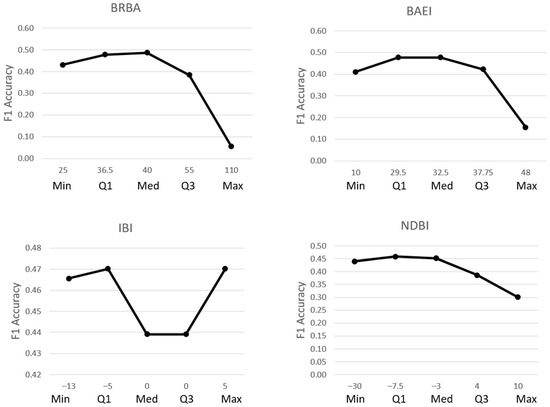
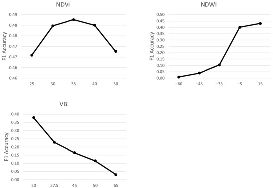
Figure 5.
For each index, average F1 accuracy is shown on the Y axis and threshold values and metric type are shown along the X axis. Average F1 accuracy results (Figure 4) are shown for results using thresholds from Table 6 to the 24 images. Thresholds with the highest F1 accuracy, represented in these graphs as the peak value, were used at globally optimal thresholds (Table 7).
Thresholds for texture were selected for testing in a different way than the built-up indices due to the way the texture metric was calculated. The texture index values were subset into 10 bins using the “Natural Breaks” tool, and the threshold represents the bin cut-off rather than a pixel value cut-off. The pixels in bins that were higher or equal to the texture threshold had a relatively higher statistical deviation from surrounding pixels and, as such, were considered relatively rougher; these were reclassified as ‘built-up’, while the pixels in lower bins that were relatively smoother were reclassified as ‘not built-up’. Given this, using the same range as the indices would have resulted in testing repeated values. Instead, four texture bin thresholds were selected for testing after observational review: the researcher preferences of 4 and 5 and an additional higher and lower bin. Texture bin thresholds of 3 through 6 were then evaluated within the workflow after the optimal thresholds for the built-up indices were established (Table 8).
2.8. Training Data Selection
After permissive masking, we reclassified index and texture rasters to binary indices using the global optimal thresholds (Table 8) such that a class value of ‘1’ indicated built-up pixels and ‘0’ indicated not built-up pixels. The binary versions of each index were summed together, creating an ensemble raster in which the cell value indicated the number of indices that considered that pixel to be built-up. A cell value of ‘6’ was the highest value, indicating unanimous agreement from the six indices that the pixel was built-up, and ‘0’ was the lowest, indicating unanimous agreement that the pixel was not built-up.
The ensemble was reclassified into three categories. Values of ‘0–2’ were classified as ‘not built-up’; ‘3’ was classified as ‘potentially confused’; and ‘4’ and greater were classified as ‘built-up’. Potentially confused areas were not used for training data. An equal stratified sampling design selected 1000 points each within the ‘not built-up’ (‘0–2’) and ‘built-up’ (‘4–6’) categories. The sample points were automatically labeled after the subset they were chosen from.
Labels were additionally corrected using a series of masking rules for texture, NDWI, and NDVI, using respective global optimal thresholds of 6, 0.15, and 0.35. (More permissive thresholds of 0.2 for NDWI and 0.5 for NDVI were used earlier in the workflow to mask ensemble inputs. Permissive values were used at that stage to reduce the number of excluded pixels in order to allow the RF model to attempt to classify spectrally mixed pixels and pixels with intermediate values. However, the stricter global default thresholds were used to correct labeling in order to avoid introducing uncertainty into the training data.) First, if a ‘built-up’ point’s texture value was below the threshold, that point’s texture value was considered too smooth to be correctly labeled and was relabeled ‘not built-up’. Inversely, a ‘not built-up’ point with a texture value above the threshold was considered too rough to be correctly labeled and was relabeled ‘built-up’. Similarly, for each of the other two indices, water and vegetation, ‘built-up’ points that scored above the global optimal threshold for NDWI or NDVI were considered too wet or green to be correctly labeled and were relabeled ‘not built-up’.
2.9. Random Forest Classifier Inputs and Settings and Automated Validation
The corrected training points were input into the RF machine learning function, in addition to the blue, green, red, NIR, and SWIR bands and the reclassified NDWI, NDVI, NDBI, BAEI, VBI, BRBA, IBI, and texture rasters. The RF settings allowed a maximum number of trees at 500, a maximum tree depth of 30, and a maximum of 2000 samples per class. The RF predicted a binary classification map of built-up and not built-up categories. The labeled ground data, which were used to develop the thresholds, were used to validate the final RF binary classification maps.
Variations of the workflow were tested to examine the sensitivity and usefulness of the texture index using texture bin thresholds of 3, 4, 5, and 6. In addition, one run was completed without the texture index in the ensemble, correction of training data, or RF input; this run included lowering the high and low ensemble bound by one from 4 and 2 to 3 and 1, as the total number of indices in consideration were reduced when texture was excluded.
3. Results
Comparison of texture layers created from each of the four 10 m VIS-NIR bands showed no difference between the three visible bands, though each showed better separability between vegetation and built-up pixels than the NIR band (Figure 3). For example, note in Figure 3 that the vegetated area between the town and river has values similar to the built-up areas when using the NIR band (top right) but is distinguishable when using the red band to create the metric (top left). The red band was selected from the three visual bands, as it is frequently provided by sensors and read in for use in other indices, but results were similar with the blue or green bands. This metric can exclude spectrally similar bare ground, which is commonly misclassified when using built-up indices (below left and right, Figure 3).
The manually chosen optimal index thresholds per image are shown in Table 5. They are summarized by minimum, maximum, median, and first and third interquartile ranges in Table 6. The summary values in Table 6 were then used to classify the imagery for all images, and classification results were tested against the ground truth points; the F1 scores for the ground truth results were calculated and listed in Table 7. These values were averaged by index threshold across the 24 images and graphed (Figure 4) to visualize at which threshold the highest average accuracy was achieved. The thresholds with the highest accuracy were collected per index as the globally optimal thresholds (Table 8).
The globally optimal thresholds were applied through the workflow (Figure 2) to mask imagery, create an ensemble of classified indices, and filter training data for an RF classifier. Four runs were conducted on all 24 images using the globally optimal index thresholds with different texture thresholds, and an additional ‘no texture’ run removed texture from the ensemble, masking, and classification (Table 8). The output was tested against the ground truth data.
The accuracy assessment for these runs resulted in an average F1 accuracy across images of 0.5304 (±0.07) and an overall accuracy of 79.95% (±4%) for the strictest texture threshold of 6. More lenient thresholds improved F1 from 0.02 to 0.08, with a tradeoff in OA from −2 to −7. A threshold of 4 provided the highest F1 of 0.6135. However, more lenient thresholds resulted in overclassification of fallow agriculture fields in images where that land cover was prevalent. Exclusion of the texture index resulted in a similar F1 of 0.5258 but a drastically lower OA of 59.21%. The inclusion of the texture index under the tested thresholds of 3–6 therefore improved the OA of the classification by a range of 14–21%.
Commission and omission errors were compared across the four texture thresholds and a no-texture option using leaf-on and leaf-off subsets (Figure 6). Error was calculated as a ratio of the number of erroneously classified validation points over the total validation points for total, commission, and omission error. The average was taken across the 24 images.
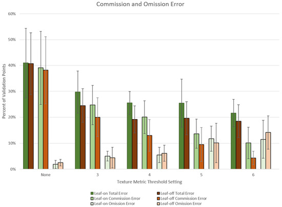
Figure 6.
Error ratios are shown for the average total, commission, and omission error for leaf-on and leaf-off subsets. Results from texture thresholds of 3, 4, 5, and 6 are compared alongside the ‘no texture’ results. Overall, texture reduced commission error at a tradeoff with omission error as the threshold increased.
The average total error decreased with the use of a texture layer at all four thresholds compared to the ‘no texture’ results (Figure 6). For the lower texture and ‘no texture’ results, total average error was driven by commission errors. A tradeoff between commission and omission error appeared to occur as the texture threshold increased. Variability also decreased in commission errors as the texture threshold increased.
Trends for the leaf-on and leaf-off subset pairs for total, commission, and omission errors were similar (Figure 7). To assign leaf-on and leaf-off dates to subsets, the date with the most vigorous visible natural vegetation from each pair was categorized as leaf-on. (Leaf-on dates are indicated with asterisks in Table 2). Total error was consistently slightly higher for leaf-on sites compared to leaf-off. However, average F1 values were 0.5426 (±0.0589) for leaf-on and 0.5182 (±0.0851) for leaf-off, with an OA of 78.37% (±3.52) and 81.53% (±4.2) (Table 9). The slight difference between subsets appears to be driven by differences in commission error (Figure 7). However, confidence intervals (CIs) at a 0.05 alpha largely overlapped the opposing mean for most pairs, suggesting little difference between leaf-on and leaf-off subsets. Exceptions are the commission error and total error at a texture threshold of 4 and commission error at a texture threshold of 6.
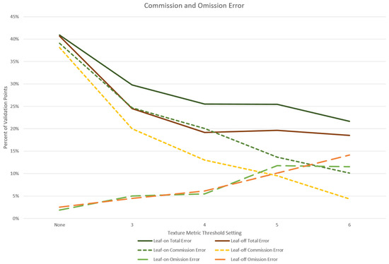
Figure 7.
The average total, commission, and omission errors are shown for leaf-on and leaf-off subsets. Each subset contains twelve images, one date from each site. Results are shown for texture thresholds of 3, 4, 5, and 6 and ‘no texture’.
Table 9.
The differences in accuracy results are presented for the workflow while using global and manually chosen thresholds, organized by the difference in F1 accuracy. The average OA accuracy was similar, while the average F1 showed a small preference for the global defaults.
To examine other land covers as possible drivers of error, proportions of land cover were estimated across the images for built-up, vegetation, water, and bare-ground land covers. Sites were labeled by dominant land cover type. Commission and omission error ratios were graphed for results at a texture threshold of 6, which had the lowest total error ratio, with color indicating the dominant land cover of that scene (Figure 8).
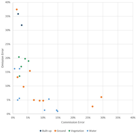
Figure 8.
Commission and omission error ratios are graphed for the 24 images. Sites are colored by dominant land cover. Many sites showed unbalanced error driven by either commission or omission error rather than a more equal combination of error types.
Results with the highest total error, >25%, showed predominantly high errors of a single type, either a majority of commission or omission errors. The two Guangzhao sites, which had the highest proportion of built-up land cover, both showed high omission error (32 and 36%, shown in black in Figure 8), along with a mountainous leaf-off scene taken over Lhasa in February (37%). These three images erroneously excluded points over dense areas with small, intermixed buildings, pavement types, and vegetation, such as residential neighborhoods and some agricultural and industrial developments. The Guangzhao sites additionally showed error over extremely large roofs with relatively uniform values, a feature that was more common in this industrial megacity than any other site in this study.
The two sites showing commission error >25% were Alice Springs’ leaf-on scene in December (30%) and Savannahket’s leaf-on scene in July (27%). Savannahket’s commission errors largely occurred over small, cleared agricultural fields with a bright signal. Error over Alice Springs, a dryland scene with sparse vegetation in leaf-on season and large areas of bare ground, included commission errors over natural areas of bare ground and highly turbid water.
Estimates of proportional cover for built-up, vegetation, water, and bare-ground land covers were also used to rank results and separate them into high, medium, and low thirds of eight scenes each. For each cover type, average results for each third were graphed along with confidence intervals (Figure 9). The CIs overlap for many compared groups, and there is little difference between the high, medium, and low groups for some categories. However, the high variation suggests a pattern of unbalanced error, which is also evident in the scatter-plot distribution (Figure 8).
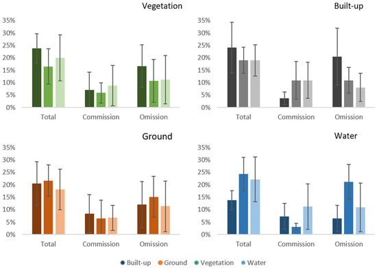
Figure 9.
Error is shown after estimates of proportional land cover were used to rank results and separate them into high, medium, and low thirds. Sites are colored by dominant land cover.
Scenes with the most water land cover (an estimated range of 50–75% for the high group, which included both dates for Mykonos, Leiden, Port-au-Prince, and Paraty) showed less total error than scenes in the middle and low groups, where water pixels were less represented. Comparing this to the water-dominated scenes graphed in Figure 8, many scenes tended to have more commission or omission error rather than a balance of both. For example, the two Leiden scenes with the highest omission error (15–16%) of the water-dominant scenes have relatively little commission error (1–2%); the omission errors largely occur over areas of small dense roofs, such as residential neighborhoods. The two water-dominant scenes with the highest commission error, Mykonos, June (15%) and Paraty, July (15%), exhibit error over natural areas of bare ground with relatively little omission error (1%). Scenes with dominant bare-ground land cover also exhibited this pattern of unbalanced error, and showed similar error classifying residential neighborhoods (Lhasa, February) and bare ground, dry grassland, and fallow agriculture (Alice Springs, December and Savannahket, July).
Vegetation and built-up dominant groups were smaller in number but tightly grouped (Figure 8). More omission errors than commission occurred in the eight scenes with the highest proportion of vegetation (which include Shobara; Riga; and Lhasa, August, which are also the five vegetation-dominant scenes, as well as Paraty, November; Savannahket, July; and Paraty, July) and the eight with the highest proportion of built-up land cover (Guangzhao, which are the only two built-up-dominant scenes, as well as Lhasa; Port-au-Prince; Shobara, December; and Riga, July) (Figure 8 and Figure 9). Of the five vegetation-dominant scenes, four had decreased total error when a lower texture threshold was applied (Shobara, December improved by 8% at a threshold of 4; Riga, October by 11% at 3; Riga, July by 9% at 4; and Lhasa, August by 3% at 5; while the fifth scene, Shobara, April, had nearly equal results at a texture level of 5) (Figure 10).
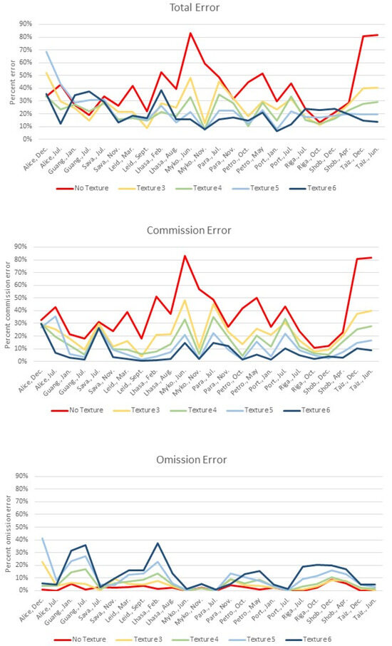
Figure 10.
Error rates are shown for total, commission, and omission errors for all 24 images for classifications. Results are shown for classifications calculated with each of four threshold options for the texture index and one ‘no texture’ option.
When total error was compared for no texture and texture thresholds of 3, 4, 5, and 6, eleven of the scenes were best classified with a texture threshold of 6 (Figure 10). The remainder benefited from a lower threshold. Of those scenes, Port-au-Prince, July and Lhasa, August performed best at a threshold of 5. Six sites (Savannahket, July; Leiden, March; Lhasa, February; Petropavl, October; Riga, July; and Shobara, December.) had the least error with a threshold of 4. Alice Springs, December had the least error at 4 or with no texture layer (33.5% total error). Four sites (Guangzhao, January and July; Leiden, September; and Riga, October) had the least error at a threshold of 3.
When considering commission error alone, all texture thresholds improved commission error at all sites in comparison to no texture (Figure 10, middle). However, this came at a tradeoff to omission error at many sites (Figure 10, lower). Both dates at the Guangzhao, Leiden, Lhasa, Petropavl, Riga, and Shobara sites showed the largest omission error. As mentioned above and in the Discussion, misclassification of residential neighborhoods was a large driver at these sites, with misclassification over agricultural and industrial buildings a lesser cause.
Comparative accuracy between manually chosen thresholds and the global defaults is presented in Table 9. Both sets were calculated using the automated workflow and the texture threshold with the highest OA, 6. On average, images show little difference in OA, 0.97% (±3.64%), and a small difference in F1, 0.0828 (±0.1027). However, the gains and losses between the two methods range widely, from 0.6104 to −0.2604 F1 and 24.28% to −20.00% OA. There are five instances where use of the global thresholds caused an F1 accuracy loss ≥0.10 and seven instances where it caused an F1 accuracy gain ≥0.10.
Manual threshold results were unexpectedly low, considering those thresholds were chosen to fit each scene (Table 9). Seven of the scenes with the greatest F1 gain (≥0.10) show gain against unexpectedly poor F1 results from manual thresholds that resulted in final RF classifications that misclassified most and, in four cases, all of the pixels as nontarget (Table 9). This may be a result of researchers systematically choosing values very different from the tested optimum global threshold for three indices: NDWI, VBI-sh, and BRBA. Researchers chose NDWI values that were, on average, 0.27 lower than the best-tested global threshold (Table 5, Table 6 and Table 7). For six out of the seven scenes that had F1 accuracy gains ≥0.10 when using the global thresholds, the researcher chose NDWI thresholds that were ≥0.50 lower than the global threshold. VBI-sh thresholds may have had a smaller influence at both extremes. Researchers chose VBI-sh values that were, on average, 0.22 higher than the best-tested global threshold. For two of the three sites that gained the most F1 accuracy from the global thresholds, in Paraty, the VBI-sh manual threshold of 0.65 was 0.45 higher than the global threshold of 0.20. For the two sites that lost the most accuracy when using global thresholds, the VBI-sh manual thresholds were close to the global threshold compared to most other scenes. Manually chosen BRBA values were, on average, 0.15 higher than the global threshold. For the two sites that lost the most accuracy when using global thresholds, manually chosen values were ≥0.20 higher than the threshold, suggesting that in a few cases, a very high BRBA value was appropriate and, without it, accuracy was affected. Figure 4 illustrates the penalty to accuracy that the nonoptimal manual thresholds had across all 24 scenes for those three indices.
Land cover type may have influenced whether a scene gained or lost accuracy with the global thresholds. Global thresholds performed better over many water-dominant sites. Although the scene with the greatest F1 gain using global indices was Guangzhao Jan., which had predominantly built-up land cover, the next six sites with the greatest F1 gain were water-dominant scenes over Paraty, Leiden, and Port-au-Prince (Table 9). NDWI was not tested at a higher threshold than 0.15, but the trend in the results suggests higher values may be more beneficial (Figure 5). The sites that lost F1 value >0.10 when using global values included one water-dominant scene, Mykonos Nov., and one vegetation scene, Riga, Jul., and were otherwise bare ground-dominant scenes (Lhasa Feb., Alice Springs Dec., Petropavl May). Like NDWI, the results of VBI-sh testing in Figure 5 suggest additional testing may be beneficial; a lower value may offer additional improvement. BRBA results showed more stabilization. While sites with a mixture of covers benefited from comparatively higher VBI-sh and BRBA in the manual thresholds, water-dominant sites tended to benefit from the higher NDWI and lower VBI-sh of the global thresholds.
When averaged across sites, using the RF with global optimal thresholds was equal to using either NDBI, BAEI, BRBA, or IBI with manually adjusted thresholds by itself and better than using VBI with manually adjusted thresholds (Table 10). The novel red-band texture metric run with manually adjusted thresholds showed equal or higher accuracy to the RF run with global optimal thresholds in all but three images (Savannakhet, November; Paraty, November.; and Port-au-Prince, July) and an average F1 of 0.6792, 0.1488 higher then the RF average F1 and 0.1738 higher than the next highest average F1, BRBA.
Table 10.
F1 values are shown for the automated RF classification using training data with global defaults in comparison to the F1 values of each index classified using the best-performing threshold for that index and imagery selected manually by researchers (Table 5). Orange indicates the RF outperformed the index by F1 ≥ 0.5 (light orange) or F1 ≥ 0.10 (dark orange), and blue indicates where the RF underperformed compared to the index alone by F1 ≥ 0.5 (light blue) or F1 ≥ 0.10 (dark blue).
However, there was a wide range in performance at individual sites. Thirteen images showed the RF with global optimal thresholds had better performance than the majority of manually adjusted indices. One site showed mostly similar performance (Savannakhet, Laos, July). The remaining ten images showed the majority of manually adjusted indices outperforming the results of the RF with global optimal thresholds.
To compare our output to output from a deep learning method, we validated our ground truth data against the Global Human Settlement (GHS) layer, a deep learning-derived dataset from Corbane et al. [55], over the same 12 sites in this study. The imagery is not a direct comparison, as the GHS was calculated over best-available pixel composites rather than specific dates, but both are from the same Sentinel-2 dataset [55]. A similar threshold was also used. Corbane et al. [55] reported a 61% and 77% OA for close and far-range transfer learning for one site, with an average Balanced Accuracy of 0.7 and an average Kappa of 0.5 when using a binary threshold of 0.2. This threshold is comparable to how researchers in this study labeled our ground truth data. Classification output is shown in Figure 11.
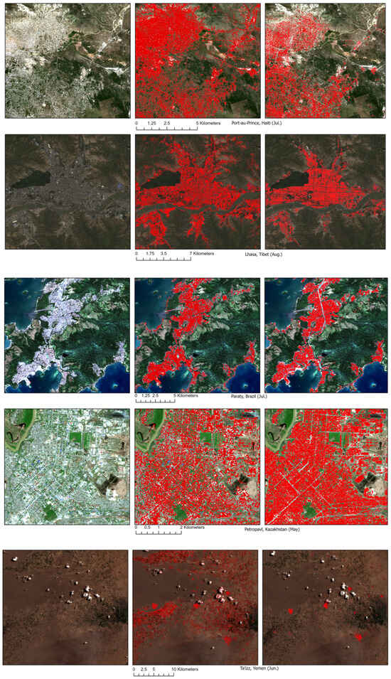
Figure 11.
Built-up classifications for subsets at five sites are shown, with the pixels classified as built-up shown in red. The true color image is shown on the left for comparison. The RF output using global optimal thresholds and a texture threshold of 6 is shown in the center. The GHS output is shown on the right.
At the same threshold of 0.2, the GHS layer provided an 88.10% (±5) OA and 0.6879 (±0.09) F1 accuracy over our 12 sites (Table 11). This surpassed the accuracy of this study’s workflow, 79.95% (±4%) OA and 0.5304 (±0.07) F1 (Table 9). Differences between GHS and this workflow per image are shown in Table 12, grouped by leaf on and leaf off images, and show an average F1 difference of 0.1575 and average OA difference of 8.15%. GHS showed much less commission error in water- and ground-dominant sites (Figure 12). Lhasa, Guangzhao, and Shobara showed lower omission error, though still higher relative to other sites.
Table 11.
Accuracy assessment is shown for the Global Human Settlement (GHS) layer, which was validated against the ground truth data for each of the twelve sites.
Table 12.
Differences in accuracy and error metrics between GHS layer and classifications from our workflow are shown. Positive values in the accuracy metric (F1, OA, precision, and recall) or negative values of the error metrics (commission and omission) indicate better performance using the HPC deep learning option.
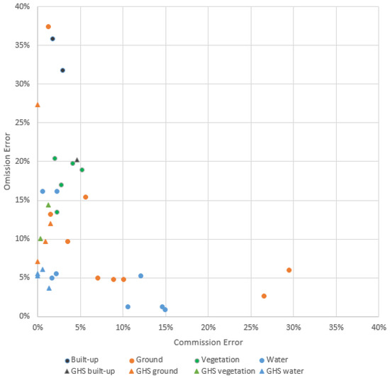
Figure 12.
GHS commission and omission error ratios for the 12 sites are added to the 24 images for comparison. Sites are colored by dominant land cover. Two sites, Alice Springs and Lhasa, had different dominant land cover seasonally and were here categorized by the leaf-off ground-dominant season. GHS showed much less commission error in water- and ground-dominant sites and smaller reductions in omission error.
4. Discussion
Our results show that when site-agnostic automation and speed are priorities for built-up area mapping, this automated workflow with globally optimal thresholds can quickly produce maps comparable to maps produced using manually adjusted thresholds. For uses where higher accuracy is needed, this process can provide a first-pass classification without user input, which can then be used to indicate how thresholds can be manually adjusted to improve output accuracy for a specific scene.
Texture was useful in reducing commission error. Total average error across the 24 sites was driven by high commission error when texture was not included. Given that, reducing commission error was a dominant concern in developing and applying the texture metric. Use of texture at any level reduced commission error.
However, reducing commission error with texture came at a tradeoff with omission error. At the highest (strictest) texture level tested, 6, omission error surpassed commission error. This tradeoff is reasonable to expect, as raising the texture threshold will cause the model to exclude more pixels from consideration as built-up training data. This exclusion may cause the model definition for built-up area to be more selective and narrow in its classification and more likely to exclude edge cases, causing omission error.
In two cases, error related to texture thresholds may be driven by the relative size of the target roofs compared to the pixel size, which influences how the texture metric’s 3 × 3 window assigns a standard deviation value. Much of the observed tradeoff omissions occurred in areas of small, close construction, such as residential neighborhoods and some agricultural and industrial buildings. This drove misclassification in the imagery with the highest omission error, the two Guangzhao sites (32 and 36% omission error) and the Lhasa, February site (37%). Texture additionally underclassified the centers of extremely large industrial buildings in Guangzhao. This may be due to roofs, in both cases, being surrounded by pixels of similar value, either the homogeneity of residential neighborhoods with similar subpixel mixing within the 3 × 3-pixel window or the homogeneity of large roofs relative to the window. This homogeneity caused the texture calculation to assign a low standard deviation value. When this value fell below the texture threshold, the texture metric excluded examples of that type of construction from the training data.
In an inverse case, strong contrast between nontarget land covers could produce high standard deviation and increase commission error. This was a dominant cause in two sites showing commission error over 25%: Alice Springs’ leaf-on scene in December (30%) and Savannahket’s leaf-on scene in July (27%). Commission error at these sites occurred near edges of fallow or recently cleared land where the 3 × 3-pixel window of analysis included pixels of different land cover. The dissimilarity within the 3 × 3 window between nontarget land covers raised the statistical deviation high enough that the texture filter did not exclude it from consideration as built-up training data.
For sites whose total error was driven by omission, error could be reduced by lowering the texture thresholds. Of the three sites with the highest omission error at a threshold of 6, the use of a texture threshold of 3 on the Guangzhao scenes lowered total error from 38% to 14% for the July date and 35% to 24% for the January date. These results slightly outperformed the ‘no texture’ option, which respectively provided a total error of 19% and 27% at those sites. A threshold of 4 reduced the total error ratio for the Lhasa Feb. image from 39% to 21%. This outperformed the ‘no texture’ option, which had 53% error. These three images showed error largely over residential neighborhoods as well as industrial and agricultural buildings. This may suggest that sites with a wider variety of construction patterns benefit from a lower texture threshold, which may allow a broader classification of built-up cover.
Existing studies achieve high accuracy while focusing on a single region, manually selecting index thresholds, or creating manually labeled training data. The creators of the BAEI tested their index against BRBA, NDBI, NBAI, and NBI over a single site with manually selected thresholds, resulting in an OA range of 70–93% [33]. The VBI-SWIR1 was tested over a single site in Tehran, Iran, along with six other spectral indices, resulting in OA ranges from 63–93% using L7 ETM+ and L8 OLI/TIR [34]. Some studies also use texture analysis methods, such as a pseudo-cross multivariate variogram (PCMV) or a gray-level co-occurrence matrix (GLCM). Bramhe et al. [3] found that including GLCM texture metrics increased OA from 84.38% to 89.29% over a single image in Uttarakhand, India. One of the GLCM metrics, variance, likely correlates to the values used in the red-band texture index used here. Feng et al. [66] found inclusion of a multiband two-date PCMV texture metric improved OA by 1.9–13.1%, resulting in ranges of 93–97% OA and 0.88–0.96 F1 over two study sites, Tianjin and Beijing, China. However, our automated RF workflow with global defaults resulted in a comparable average OA of 79.95% (±4) and 0.5304 (±0.07) F1 across twelve globally distributed sites for two dates, each without manual adjustment.
Greater accuracy might be achieved through deep learning methods. However, these methods require technical expertise and equipment, such as dedicated computational infrastructure for high-capacity processing, which is not yet universally available. Here, the GHS layer provided an 88.10% (±5) OA and 0.6879 (±0.09) F1 accuracy over our 12 sites, surpassing the accuracy of this study’s workflow. This may not be a direct comparison, as imagery inputs varied; for this workflow, L2 Sentinel-2 tiles were chosen to include geographic and seasonal variation, while the GHS layer had been calculated over best-available pixel composites from Sentinel-2 imagery. However, a larger concern for general application may be that Corbane et al. [55] leveraged an optimized fast parallel processing system with multi-petabyte scale storage, which is not commonly available and may limit replication and updating for some users. Depending on the application, a more computationally lightweight solution, such as that demonstrated in this study, may achieve similar accuracy with fewer computational requirements.
While overall accuracy is a more commonly reported metric and thus provided by this study for comparison, OA does not penalize underclassifying a rarely occurring target (i.e., built-up pixels), particularly when ground truth sample sizes are uneven. The stricter F1 metric was more useful due to the balance F1 provides between precision and recall. For example, an output map that classified every pixel as not built-up could have a high OA score in a scene where the target is rare due to the perfect accuracy it provides of the not built-up pixels by overclassifying. However, the low precision and recall will be evidenced in a correspondingly low F1. This occurred during the manual threshold testing in Leiden, Paraty Nov., and Guangzhao Jan., four sites that had reasonable OA scores but F1 scores of zero (Table 9). F1 is provided in Feng et al. [66], which had an 0.88–0.96 F1 over two study sites using two-date multiband texture. Y. Zheng et al. [23] also reported an F1 ranging from 0.90 to 0.95 over three dates over a single urban region. The latter study combined NDVI, NDWI, NDBI, and NPP-VIIRS NTL with manually selected thresholds to create an Enhanced Nighttime Light Urban Index. While our automated RF workflow with global defaults has a lower average F1 than these studies, this work may provide useful default thresholds and a simpler workflow for automated mapping across all sites when manual and single-site customization is prohibitive.
The workflow’s use of an RF classifier has a longer runtime than those using only spectral indexes. However, for 13 out of 24 images, the automated workflow with defaults outperformed the F1 score on the majority of single built-up indices with manually chosen defaults by ≥0.10 and performed similarly or better on the Savannakhet, Laos, July imagery (Table 10). This indicates that for half the images, the RF automation with globally optimal defaults outperformed traditional methods of single-index classifications, even when thresholds were manually set, which can be time-consuming to complete. The default thresholds from this study enable an alternative to time-consuming manual examination of thresholds for larger-scale assessments.
Adding texture to the workflow using thresholds from 3–6 increased the OA by 14–21% without changing F1 accuracy, showing decreasing misclassification of nontarget land cover. In addition, texture was the only tested index that most consistently outperformed the RF with global defaults when tested as a single-index classification using manually selected thresholds (Table 10, last column).
Although the advantage of using texture has been demonstrated, the texture settings offer a nonlinear tradeoff between commission and omission error (Figure 6, Figure 7, Figure 8 and Figure 9). Results using lower texture thresholds showed better classification of built-up areas but overclassification of fallow farmland, beaches, and bare ground. Allowing overclassification improved F1 accuracy while lowering OA, suggesting a nonlinear tradeoff, which may or may not be desirable depending on the user’s purpose. The red-band texture metric likely performs best in areas with balanced land cover and would likely perform less accurately in scenes with homogenous landscapes (e.g., 90% built-up area) due to the use of natural breaks clustering, and alternative thresholds may be required in such cases. However, even in areas such as the Yemen site in Figure 11, the metric made clusters of built-up area visible despite scattered misclassification in mountainous areas. This suggests an investigation of the relationship between target land cover patterns and pixel size that may influence accuracy.
There was little difference in accuracy when results were subset into leaf-on and leaf-off images. Despite efforts to choose seasonally opposed images, images from the same site may have similarities between dates or conflicting vegetation patterns due to land use, climate, or image availability. For example, leaf-off scenes in Leiden and Ta’izz contain green agricultural fields, while leaf-on scenes have fallow fields; Guangzhou and other sites have mild winters and did not exhibit much leaf senescence; and Shobara had cloud cover, limiting seasonal representation. Some sites had similar amounts of vegetation on both dates but over different locations, possibly due to dry summer seasons (Mykonos) or crop rotation (Shobara). In many scenes, fallow agricultural fields contributed to bare-ground pixels in leaf-on scenes when natural areas gained vegetation. These contradicting patterns of green-up between natural and agricultural vegetation may have contributed to the similarity in accuracy metrics between leaf-on and leaf-off scenes, regardless of the effect of vegetation on spectral separability.
Results here suggested that a lower texture threshold reduced total error in vegetation-dominant scenes. Though some commission error occurred in areas where standard deviation values were higher, such as where sparse vegetation occurred within natural areas of bare ground (Alice Springs) or near edges of agriculture fields (Savannakhet), vegetation-dominant scenes showed predominantly omission error. This omission error was likely caused by spectral mixing with vegetation in built-up areas such as residential neighborhoods and smaller buildings and roads mixed into agricultural land cover. A more permissive texture threshold improved results. Additionally, although a more permissive NDVI threshold might be expected to have a similar effect, when considering that a small range of NDVI values was tested against ground truth outside the workflow (0.4 and 0.5) and reported in Figure 4, a more permissive NDVI did not show much change from the 0.35 global threshold.
The lower total error of water-dominated scenes may reflect that scenes with greater water area tended to have water bodies with high separability, such as deep or clear water. Scenes with less water area not only had more land cover that was more likely to be miscategorized than water, such as bare ground, fallow agriculture, and small buildings, but smaller shallower water bodies with spectrally mixed pixels that were difficult to consistently categorize, such as shallow turbid rivers or ephemeral wetlands.
Future work could benefit from including a larger set of sites chosen without subjective review. While random stratified sampling was used within sites, and sites were selected considering a range of HDI and development densities, researchers made a subjective choice of scene tiles through exploratory review. The intention was to capture imagery featuring typical intractable classification problems, which may not be represented well in random sampling, in order to test the performance of the indices and texture metric more robustly. However, a more objective method and a larger number of observations may provide additional confidence.
Explicit inclusion of ecological context could improve sampling as well. Although our samples included examples of most subarctic biomes, four biomes were not represented, including boreal forests and temperate conifer forest biomes. These biomes may introduce unanticipated complexity that is different from tested forested biomes and contain many population centers; thus, they should be included in future testing.
All imagery was collected before the European Space Agency’s Processing Baseline 04.00 update improved the Scene Classification Layer (SCL) algorithm; as such, masking cloud and shadow using the pre-change SCL was tested but performed poorly and was not used in the final version of the workflow [67]. Using this SCL mask lowered the average F1 accuracy of the global defaults by 0.11; removing the SCL mask improved performance at all sites. One of the main causes of error using the SCL was its masking of bright white roofs; the SCL update cited improvements in cloud detection over areas with bright targets, which may offer advantages for including SCL masking in this workflow in the future but not when working with imagery processed before the 25 June 2022 SCL update [67]. Additionally, the improved performance of the GHS may be due in part to its calculation over best-pixel-available composites, a method designed to reduce cloud interference [55]. This is valuable but requires building a time series of imagery compatible with the purpose of the application. Best-available-pixel composites may not be practical for all mapping applications, such as mapping land cover change or supporting immediate disaster response, as the best-available pixel may not be the most recent or most representative of current ground conditions.
5. Conclusions
This study combined an ensemble of built-up indices and nontarget land cover masks with globally optimized thresholds to select training data automatically for an RF classifier, quickly producing a binary map without time-consuming user input. The globally optimized thresholds were chosen after testing a range of values taken across two different seasons of imagery from 12 sites (24 images). Globally optimized thresholds were found to be: −0.08 for NDBI, 0.31 for BAEI, 0.20 for VBI-shadow, 0.40 for BRBA, −0.05 for IBI-adjusted, 0.35 for NDVI, and 0.15 for NDWI, and 6 for the texture metric.
The use of these global defaults was found to improve accuracy when nontarget bare-ground pixels were removed using a novel texture metric that incorporates rates of value variation within the immediate surrounding pixels. Inclusion of texture increased the workflow’s overall accuracy by 14–21%, depending on the threshold used. More lenient thresholds improved F1 from 0.02 to 0.08, though a tradeoff in OA from −2 to −7 resulted in overclassification of fallow agriculture fields.
Validation was conducted on subsets of stratified random points over two dates of imagery across 12 internationally distributed sites representing a majority of, but not all of, Earth’s biomes. The accuracy assessment resulted in an average F1 accuracy of 0.5304 (±0.07) and overall accuracy of 79.95% (±0.04). For 14 of the 24 images, the global defaults perform equally or better than when the same workflow was used with manually chosen site-specific thresholds. This automated method offers end-users a quick approach for built-up area mapping, providing comparable accuracy without time-consuming user-selected thresholds or training data.
Author Contributions
Conceptualization, M.C.M.; Methodology, M.C.M., A.W.H.G., S.J.B., S.L.L. and K.L.; Validation, M.C.M., A.W.H.G., S.J.B., S.L.L. and K.L.; Formal Analysis, M.C.M.; Data Curation, M.C.M., A.W.H.G., S.J.B., K.L. and S.L.L.; Writing—Original Draft Preparation, M.C.M.; Writing—Review and Editing, M.C.M., A.W.H.G., S.J.B., K.L. and S.L.L.; Visualization, M.C.M., S.L.L. and K.L.; Supervision, S.J.B. and M.C.M.; Project Administration, S.J.B. All authors have read and agreed to the published version of the manuscript.
Funding
Funds for this research were provided by the U.S. Army Corps of Engineers (USACE), Engineer Research and Development Center (ERDC), Geospatial Research & Engineering Research & Development Area. The use of trade, product, or firm names in this document is for descriptive purposes only and does not imply endorsement by the U.S. Government. The tests described and the resulting data presented herein, unless otherwise noted, are based upon work conducted by the US Army Engineer Research and Development Center supported under PE 0633463, Project AU1 ’Tactical Geospatial Information Capabilities’, Task ’Enhanced Terrain Processing’. Permission was granted by the Office of the Technical Director, Geospatial Research Laboratory, to publish this information. The findings of this report are not to be construed as an official Department of the Army position unless so designated by other authorized documents.
Data Availability Statement
Data are contained within the article.
Acknowledgments
The authors would like to particularly thank the following USACE staff: Elena Sava for discussion supporting the conceptual development of the texture layer, and Nicole Wayant and Jean Nelson for funding procurement and project management.
Conflicts of Interest
The funders had no role in the design of the study; in the collection, analyses, or interpretation of data; in the writing of the manuscript; or in the decision to publish the results.
References
- Borana, S.L.; Yadav, S.K. Chapter 10-Urban Land-Use Susceptibility and Sustainability—Case Study. In Water, Land, and Forest Susceptibility and Sustainability; Chatterjee, U., Pradhan, B., Kumar, S., Saha, S., Zakwan, M., Fath, B.D., Fiscus, D., Eds.; Science of Sustainable Systems; Academic Press: Amsterdam, The Netherlands, 2023; Volume 2, pp. 261–286. ISBN 978-0-443-15847-6. [Google Scholar]
- Tan, Y.; Xiong, S.; Li, Y. Automatic Extraction of Built-Up Areas From Panchromatic and Multispectral Remote Sensing Images Using Double-Stream Deep Convolutional Neural Networks. IEEE J. Sel. Top. Appl. Earth Obs. Remote Sens. 2018, 11, 3988–4004. [Google Scholar] [CrossRef]
- Bramhe, V.S.; Ghosh, S.K.; Garg, P.K. Extraction of Built-Up Area by Combining Textural Features and Spectral Indices from LANDSAT-8 Multispectral Image. Int. Arch. Photogramm. Remote Sens. Spat. Inf. Sci. 2018, XLII–5, 727–733. [Google Scholar] [CrossRef]
- Kaur, R.; Pandey, P. A Review on Spectral Indices for Built-up Area Extraction Using Remote Sensing Technology. Arab. J. Geosci. 2022, 15, 391. [Google Scholar] [CrossRef]
- Taubenböck, H.; Weigand, M.; Esch, T.; Staab, J.; Wurm, M.; Mast, J.; Dech, S. A New Ranking of the World’s Largest Cities—Do Administrative Units Obscure Morphological Realities? Remote Sens. Environ. 2019, 232, 111353. [Google Scholar] [CrossRef]
- Huang, X.; Li, J.; Yang, J.; Zhang, Z.; Li, D.; Liu, X. 30 m Global Impervious Surface Area Dynamics and Urban Expansion Pattern Observed by Landsat Satellites: From 1972 to 2019. Sci. China Earth Sci. 2021, 64, 1922–1933. [Google Scholar] [CrossRef]
- Mirzaei, M.; Verrelst, J.; Arbabi, M.; Shaklabadi, Z.; Lotfizadeh, M. Urban Heat Island Monitoring and Impacts on Citizen’s General Health Status in Isfahan Metropolis: A Remote Sensing and Field Survey Approach. Remote Sens. 2020, 12, 1350. [Google Scholar] [CrossRef] [PubMed]
- Shi, H.; Xian, G.; Auch, R.; Gallo, K.; Zhou, Q. Urban Heat Island and Its Regional Impacts Using Remotely Sensed Thermal Data—A Review of Recent Developments and Methodology. Land 2021, 10, 867. [Google Scholar] [CrossRef]
- Basu, R. High Ambient Temperature and Mortality: A Review of Epidemiologic Studies from 2001 to 2008. Environ. Health 2009, 8, 40. [Google Scholar] [CrossRef]
- Gasparrini, A.; Guo, Y.; Hashizume, M.; Lavigne, E.; Zanobetti, A.; Schwartz, J.; Tobias, A.; Tong, S.; Rocklöv, J.; Forsberg, B.; et al. Mortality Risk Attributable to High and Low Ambient Temperature: A Multicountry Observational Study. Lancet 2015, 386, 369–375. [Google Scholar] [CrossRef]
- Song, Y.; Huang, B.; He, Q.; Chen, B.; Wei, J.; Mahmood, R. Dynamic Assessment of PM2.5 Exposure and Health Risk Using Remote Sensing and Geo-Spatial Big Data. Environ. Pollut. 2019, 253, 288–296. [Google Scholar] [CrossRef]
- Sakti, A.D.; Anggraini, T.S.; Ihsan, K.T.N.; Misra, P.; Trang, N.T.Q.; Pradhan, B.; Wenten, I.G.; Hadi, P.O.; Wikantika, K. Multi-Air Pollution Risk Assessment in Southeast Asia Region Using Integrated Remote Sensing and Socio-Economic Data Products. Sci. Total Environ. 2023, 854, 158825. [Google Scholar] [CrossRef]
- Doernberg, A.; Weith, T. Urban-Rural Interrelations—A Challenge for Sustainable Land Management. In Sustainable Land Management in a European Context: A Co-Design Approach; Weith, T., Barkmann, T., Gaasch, N., Rogga, S., Strauß, C., Zscheischler, J., Eds.; Human-Environment Interactions; Springer International Publishing: Cham, Switzerland, 2021; pp. 101–124. ISBN 978-3-030-50841-8. [Google Scholar]
- Zheng, Q.; Weng, Q.; Wang, K. Characterizing Urban Land Changes of 30 Global Megacities Using Nighttime Light Time Series Stacks. ISPRS J. Photogramm. Remote Sens. 2021, 173, 10–23. [Google Scholar] [CrossRef]
- Slonecker, E.T.; Jennings, D.B.; Garofalo, D. Remote Sensing of Impervious Surfaces: A Review. Remote Sens. Rev. 2001, 20, 227–255. [Google Scholar] [CrossRef]
- Weng, Q. Remote Sensing of Impervious Surfaces in the Urban Areas: Requirements, Methods, and Trends. Remote Sens. Environ. 2012, 117, 34–49. [Google Scholar] [CrossRef]
- See, L.; Georgieva, I.; Duerauer, M.; Kemper, T.; Corbane, C.; Maffenini, L.; Gallego, J.; Pesaresi, M.; Sirbu, F.; Ahmed, R.; et al. A Crowdsourced Global Data Set for Validating Built-up Surface Layers. Sci. Data 2022, 9, 13. [Google Scholar] [CrossRef]
- Hu, X.; Weng, Q. Estimating Impervious Surfaces from Medium Spatial Resolution Imagery Using the Self-Organizing Map and Multi-Layer Perceptron Neural Networks. Remote Sens. Environ. 2009, 113, 2089–2102. [Google Scholar] [CrossRef]
- Zhang, H.; Lin, H.; Wang, Y. A New Scheme for Urban Impervious Surface Classification from SAR Images. ISPRS J. Photogramm. Remote Sens. 2018, 139, 103–118. [Google Scholar] [CrossRef]
- Zhang, J.; Li, P.; Wang, J. Urban Built-Up Area Extraction from Landsat TM/ETM+ Images Using Spectral Information and Multivariate Texture. Remote Sens. 2014, 6, 7339–7359. [Google Scholar] [CrossRef]
- Liang, X.; Lin, Y.; Zhang, H. Mapping Urban Impervious Surface With an Unsupervised Approach Using Interferometric Coherence of SAR Images. IEEE J. Sel. Top. Appl. Earth Obs. Remote Sens. 2022, 15, 2734–2744. [Google Scholar] [CrossRef]
- Levin, N.; Kyba, C.C.M.; Zhang, Q.; Sánchez De Miguel, A.; Román, M.O.; Li, X.; Portnov, B.A.; Molthan, A.L.; Jechow, A.; Miller, S.D.; et al. Remote Sensing of Night Lights: A Review and an Outlook for the Future. Remote Sens. Environ. 2020, 237, 111443. [Google Scholar] [CrossRef]
- Zheng, Y.; Tang, L.; Wang, H. An Improved Approach for Monitoring Urban Built-up Areas by Combining NPP-VIIRS Nighttime Light, NDVI, NDWI, and NDBI. J. Clean. Prod. 2021, 328, 129488. [Google Scholar] [CrossRef]
- Im, J.; Lu, Z.; Rhee, J.; Quackenbush, L.J. Impervious Surface Quantification Using a Synthesis of Artificial Immune Networks and Decision/Regression Trees from Multi-Sensor Data. Remote Sens. Environ. 2012, 117, 102–113. [Google Scholar] [CrossRef]
- Fan, W.; Wu, C.; Wang, J. Improving Impervious Surface Estimation by Using Remote Sensed Imagery Combined with Open Street Map Points-of-Interest (POI) Data. IEEE J. Sel. Top. Appl. Earth Obs. Remote Sens. 2019, 12, 4265–4274. [Google Scholar] [CrossRef]
- Parekh, J.R.; Poortinga, A.; Bhandari, B.; Mayer, T.; Saah, D.; Chishtie, F. Automatic Detection of Impervious Surfaces from Remotely Sensed Data Using Deep Learning. Remote Sens. 2021, 13, 3166. [Google Scholar] [CrossRef]
- Ding, Q.; Shao, Z.; Huang, X.; Altan, O.; Hu, B. Time-Series Land Cover Mapping and Urban Expansion Analysis Using OpenStreetMap Data and Remote Sensing Big Data: A Case Study of Guangdong-Hong Kong-Macao Greater Bay Area, China. Int. J. Appl. Earth Obs. Geoinf. 2022, 113, 103001. [Google Scholar] [CrossRef]
- Forget, Y.; Linard, C.; Gilbert, M. Supervised Classification of Built-Up Areas in Sub-Saharan African Cities Using Landsat Imagery and OpenStreetMap. Remote Sens. 2018, 10, 1145. [Google Scholar] [CrossRef]
- Grippa, T.; Georganos, S.; Zarougui, S.; Bognounou, P.; Diboulo, E.; Forget, Y.; Lennert, M.; Vanhuysse, S.; Mboga, N.; Wolff, E. Mapping Urban Land Use at Street Block Level Using OpenStreetMap, Remote Sensing Data, and Spatial Metrics. IJGI 2018, 7, 246. [Google Scholar] [CrossRef]
- Zhang, X.; Liu, L.; Wu, C.; Chen, X.; Gao, Y.; Xie, S.; Zhang, B. Development of a Global 30 m Impervious Surface Map Using Multisource and Multitemporal Remote Sensing Datasets with the Google Earth Engine Platform. Earth Syst. Sci. Data 2020, 12, 1625–1648. [Google Scholar] [CrossRef]
- Gao, F.; De Colstoun, E.B.; Ma, R.; Weng, Q.; Masek, J.G.; Chen, J.; Pan, Y.; Song, C. Mapping Impervious Surface Expansion Using Medium-Resolution Satellite Image Time Series: A Case Study in the Yangtze River Delta, China. Int. J. Remote Sens. 2012, 33, 7609–7628. [Google Scholar] [CrossRef]
- Zhang, T.; Huang, X. Monitoring of Urban Impervious Surfaces Using Time Series of High-Resolution Remote Sensing Images in Rapidly Urbanized Areas: A Case Study of Shenzhen. IEEE J. Sel. Top. Appl. Earth Obs. Remote Sens. 2018, 11, 2692–2708. [Google Scholar] [CrossRef]
- Bouzekri, S.; Lasbet, A.A.; Lachehab, A. A New Spectral Index for Extraction of Built-Up Area Using Landsat-8 Data. J. Indian Soc. Remote Sens. 2015, 43, 867–873. [Google Scholar] [CrossRef]
- Ezimand, K.; Kakroodi, A.A.; Kiavarz, M. The Development of Spectral Indices for Detecting Built-up Land Areas and Their Relationship with Land-Surface Temperature. Int. J. Remote Sens. 2018, 39, 8428–8449. [Google Scholar] [CrossRef]
- Firozjaei, M.K.; Sedighi, A.; Kiavarz, M.; Qureshi, S.; Haase, D.; Alavipanah, S.K. Automated Built-Up Extraction Index: A New Technique for Mapping Surface Built-Up Areas Using LANDSAT 8 OLI Imagery. Remote Sens. 2019, 11, 1966. [Google Scholar] [CrossRef]
- Waqar, M.M.; Mirza, J.F.; Mumtaz, R.; Hussain, E. Development of New Indices for Extraction of Built-Up Area & Bare Soil from Landsat Data. Open Access Sci. Rep. 2012, 1, 4. [Google Scholar]
- Xu, H. A New Index for Delineating Built-up Land Features in Satellite Imagery. Int. J. Remote Sens. 2008, 29, 4269–4276. [Google Scholar] [CrossRef]
- Zha, Y.; Gao, J.; Ni, S. Use of Normalized Difference Built-up Index in Automatically Mapping Urban Areas from TM Imagery. Int. J. Remote Sens. 2003, 24, 583–594. [Google Scholar] [CrossRef]
- Haralick, R.M.; Shanmugam, K.; Dinstein, I. Textural Features for Image Classification. IEEE Trans. Syst. Man Cybern. 1973, SMC-3, 610–621. [Google Scholar] [CrossRef]
- Weszka, J.S.; Dyer, C.R.; Rosenfeld, A. A Comparative Study of Texture Measures for Terrain Classification. IEEE Trans. Syst. Man Cybern. 1976, SMC-6, 269–285. [Google Scholar] [CrossRef]
- Irons, J.R.; Petersen, G.W. Texture Transforms of Remote Sensing Data. Remote Sens. Environ. 1981, 11, 359–370. [Google Scholar] [CrossRef]
- Chen, Z.; Chen, J.; Shi, P.; Tamura, M. An IHS-Based Change Detection Approach for Assessment of Urban Expansion Impact on Arable Land Loss in China. Int. J. Remote Sens. 2003, 24, 1353–1360. [Google Scholar] [CrossRef]
- Witharana, C.; Civco, D. Twelve Data Fusion Algorithms for Use in Rapid Damage Mapping Workflows: An Evaluation. J. Geol. Soc. Sri Lanka 2013, 15, 111–128. [Google Scholar]
- Pesaresi, M.; Politis, P. GHS-BUILT-S R2023A-GHS Built-Up Surface Grid, Derived from Sentinel2 Composite and Landsat, Multitemporal (1975–2030). 2023. Available online: https://ghslsys.jrc.ec.europa.eu/ghs_buS2023.php (accessed on 19 January 2024). [CrossRef]
- Xu, H. Analysis of Impervious Surface and Its Impact on Urban Heat Environment Using the Normalized Difference Impervious Surface Index (NDISI). Photogramm. Eng. Remote Sens. 2010, 76, 557–565. [Google Scholar] [CrossRef]
- Chen, J.; Yang, K.; Chen, S.; Yang, C.; Zhang, S.; He, L. Enhanced Normalized Difference Index for Impervious Surface Area Estimation at the Plateau Basin Scale. J. Appl. Rem. Sens. 2019, 13, 1. [Google Scholar] [CrossRef]
- Sun, Z.; Wang, C.; Guo, H.; Shang, R. A Modified Normalized Difference Impervious Surface Index (MNDISI) for Automatic Urban Mapping from Landsat Imagery. Remote Sens. 2017, 9, 942. [Google Scholar] [CrossRef]
- Lasko, K.; Maloney, M.C.; Becker, S.J.; Griffin, A.W.H.; Lyon, S.L.; Griffin, S.P. Automated Training Data Generation from Spectral Indexes for Mapping Surface Water Extent with Sentinel-2 Satellite Imagery at 10 m and 20 m Resolutions. Remote Sens. 2021, 13, 4531. [Google Scholar] [CrossRef]
- Adugna, T.; Xu, W.; Fan, J. Comparison of Random Forest and Support Vector Machine Classifiers for Regional Land Cover Mapping Using Coarse Resolution FY-3C Images. Remote Sens. 2022, 14, 574. [Google Scholar] [CrossRef]
- Belgiu, M.; Drăguţ, L. Random Forest in Remote Sensing: A Review of Applications and Future Directions. ISPRS J. Photogramm. Remote Sens. 2016, 114, 24–31. [Google Scholar] [CrossRef]
- McCarty, D.A.; Kim, H.W.; Lee, H.K. Evaluation of Light Gradient Boosted Machine Learning Technique in Large Scale Land Use and Land Cover Classification. Environments 2020, 7, 84. [Google Scholar] [CrossRef]
- Abdi, A.M. Land Cover and Land Use Classification Performance of Machine Learning Algorithms in a Boreal Landscape Using Sentinel-2 Data. GISci. Remote Sens. 2020, 57, 1–20. [Google Scholar] [CrossRef]
- Ramdani, F.; Furqon, M.T. The Simplicity of XGBoost Algorithm versus the Complexity of Random Forest, Support Vector Machine, and Neural Networks Algorithms in Urban Forest Classification. F1000Research 2022, 11, 1069. [Google Scholar] [CrossRef]
- Georganos, S.; Grippa, T.; Vanhuysse, S.; Lennert, M.; Shimoni, M.; Wolff, E. Very High Resolution Object-Based Land Use–Land Cover Urban Classification Using Extreme Gradient Boosting. IEEE Geosci. Remote Sens. Lett. 2018, 15, 607–611. [Google Scholar] [CrossRef]
- Corbane, C.; Syrris, V.; Sabo, F.; Politis, P.; Melchiorri, M.; Pesaresi, M.; Soille, P.; Kemper, T. Convolutional Neural Networks for Global Human Settlements Mapping from Sentinel-2 Satellite Imagery. Neural Comput. Applic. 2021, 33, 6697–6720. [Google Scholar] [CrossRef]
- Ma, L.; Liu, Y.; Zhang, X.; Ye, Y.; Yin, G.; Johnson, B.A. Deep Learning in Remote Sensing Applications: A Meta-Analysis and Review. ISPRS J. Photogramm. Remote Sens. 2019, 152, 166–177. [Google Scholar] [CrossRef]
- Jozdani, S.E.; Johnson, B.A.; Chen, D. Comparing Deep Neural Networks, Ensemble Classifiers, and Support Vector Machine Algorithms for Object-Based Urban Land Use/Land Cover Classification. Remote Sens. 2019, 11, 1713. [Google Scholar] [CrossRef]
- Gorelick, N.; Hancher, M.; Dixon, M.; Ilyushchenko, S.; Thau, D.; Moore, R. Google Earth Engine: Planetary-Scale Geospatial Analysis for Everyone. Remote Sens. Environ. 2017, 202, 18–27. [Google Scholar] [CrossRef]
- United Nations Development Programme (Ed.) Uncertain Times, Unsettled Lives: Shaping Our Future in a Transforming World; Human development report; United Nations Development Programme: New York, NY, USA, 2022; ISBN 978-92-1-126451-7. [Google Scholar]
- Dinerstein, E.; Olson, D.; Joshi, A.; Vynne, C.; Burgess, N.D.; Wikramanayake, E.; Hahn, N.; Palminteri, S.; Hedao, P.; Noss, R.; et al. An Ecoregion-Based Approach to Protecting Half the Terrestrial Realm. BioScience 2017, 67, 534–545. [Google Scholar] [CrossRef] [PubMed]
- Tucker, C.J. Red and Photographic Infrared Linear Combinations for Monitoring Vegetation. Remote Sens. Environ. 1979, 8, 127–150. [Google Scholar] [CrossRef]
- McFeeters, S.K. The Use of the Normalized Difference Water Index (NDWI) in the Delineation of Open Water Features. Int. J. Remote Sens. 1996, 17, 1425–1432. [Google Scholar] [CrossRef]
- Olofsson, P.; Foody, G.M.; Herold, M.; Stehman, S.V.; Woodcock, C.E.; Wulder, M.A. Good Practices for Estimating Area and Assessing Accuracy of Land Change. Remote Sens. Environ. 2014, 148, 42–57. [Google Scholar] [CrossRef]
- Chinchor, N. MUC-4 Evaluation Metrics. In Proceedings of the Fourth Message Uunderstanding Conference (MUC-4), McLean, VA, USA, 16–18 June 1992. [Google Scholar]
- van Rijsbergen, C.J. Information Retrieval, 2nd ed.; Buttersworths: London, UK, 1979. [Google Scholar]
- Feng, X.; Li, P.; Cheng, T. Detection of Urban Built-Up Area Change From Sentinel-2 Images Using Multiband Temporal Texture and One-Class Random Forest. IEEE J. Sel. Top. Appl. Earth Obs. Remote Sens. 2021, 14, 6974–6986. [Google Scholar] [CrossRef]
- European Space Agency Copernicus Sentinel-2: Major Products Upgrade Upcoming. Available online: https://copernicus.eu/-/copernicus-sentinel-2-major-products-upgrade-upcoming (accessed on 24 May 2023).
Disclaimer/Publisher’s Note: The statements, opinions and data contained in all publications are solely those of the individual author(s) and contributor(s) and not of MDPI and/or the editor(s). MDPI and/or the editor(s) disclaim responsibility for any injury to people or property resulting from any ideas, methods, instructions or products referred to in the content. |
© 2024 by the authors. Licensee MDPI, Basel, Switzerland. This article is an open access article distributed under the terms and conditions of the Creative Commons Attribution (CC BY) license (https://creativecommons.org/licenses/by/4.0/).