Abstract
Against the background of climate warming, marine heatwaves (MHWs) and terrestrial drought events have become increasingly frequent in recent decades. However, the combined effects of MHWs and terrestrial drought on CO2 uptake in marginal seas are still unclear. The East China Sea (ECS) experienced an intense and long-lasting MHW accompanied by an extreme terrestrial drought in the Changjiang basin in the summer of 2022. In this study, we employed multi-source satellite remote sensing products to reveal the patterns, magnitude, and potential drivers of CO2 flux changes in the ECS resulting from the compounding MHW and terrestrial drought extremes. The CO2 uptake of the ECS reduced by 17.0% (1.06 Tg C) in the latter half of 2022 and the Changjiang River plume region shifted from a CO2 sink to a source (releasing 0.11 Tg C) in July-September. In the majority of the ECS, the positive sea surface temperature (SST) anomaly during the MHW diminished the solubility of CO2 in seawater, thereby reducing CO2 uptake. Moreover, the reduction in nutrient input associated with terrestrial drought, which is unfavorable to phytoplankton growth, further reduced the capacity of CO2 uptake. Meanwhile, the CO2 sink doubled for the offshore waters of the ECS continental shelf in July-September 2022, indicating the complexity and heterogeneity of the impacts of extreme climatic events in marginal seas. This study is of great significance in improving the estimation results of CO2 fluxes in marginal seas and understanding sea–air CO2 exchanges against the background of global climate change.
1. Introduction
Marginal seas play a vital role in the global carbon cycle. Previous studies have reported that, globally, marginal seas take up carbon dioxide (CO2) from the atmosphere by 210–450 Tg C per year (1 Tg = 1012 g), accounting for 7.24–15.52% of the total oceanic carbon sink, albeit with considerable uncertainty [1,2]. These large uncertainties stem from divergent sampling datasets, procedural variations in processing, and the calculation methodologies employed to estimate CO2 exchange in marginal seas [3,4]. Concurrently, anthropogenic climate change modulates carbon sequestration in marginal seas by altering phytoplankton productivity, CO2 solubility, and water column stratification [5]. Hence, to refine the understanding of the global carbon cycle, it is imperative to elucidate the impacts of climate change on carbon cycling within marginal seas, particularly those receiving a great deal of terrigenous materials from input rivers.
CO2 uptake in marginal seas is co-determined by numerous factors, including riverine inputs, biological processes, and thermodynamic effects. Among these, input rivers discharge not only carbon but also nutrients into marginal seas. It has been reported that global rivers output approximately 950 Tg of carbon per year, along with 37–66 Tg of nitrogen, 4–11 Tg of phosphorus, and 340–380 Tg of silicate [6,7]. Upon entering marginal seas, most of the terrigenous organic and inorganic carbon is transformed into CO2 via photochemical oxidation, microbial respiration, and geochemical equilibrium processes [7,8]. Moreover, most of the nutrients are used for phytoplankton production, which consumes dissolved CO2 to produce organic carbon [6]. Consequently, global marginal seas are commonly characterized by high chlorophyll-a (Chl-a) concentration and atmospheric CO2 uptake [9]. Additionally, the thermodynamic process can change the upper mixing layer depth, which further determines the vertical exchanges of carbon and nutrients with the subsurface waters [10,11].
Against the background of climate warming, marine heatwaves (MHWs) and terrestrial drought events have occurred frequently and increasingly in recent decades [5,12]. MHWs can influence sea–air CO2 exchange by changing the mixing layer depth, phytoplankton community structure, and decreasing CO2 solubility [5,13]. Concurrently, terrestrial droughts diminish the riverine inputs of water, carbon, and nutrients into oceans, thereby impacting CO2 fluxes and phytoplankton growth in marginal seas [8,14]. For the global open ocean, it is reported that persistent MHWs caused a 40% reduction in CO2 emissions in the Pacific Tropics and a 29% decrease in the CO2 sink in the North Pacific during the period of 1985–2017 [5]. The same changes might be occurring in the CO2 uptake in marginal seas, but regional and/or global studies are still required to verify this, especially for coastal oceans impacted by both terrestrial droughts and MHWs.
The East China Sea (ECS) is a typical marginal sea where the carbon cycle is highly regulated by riverine input from the Changjiang River in tandem with biological carbon sequestration and hydrodynamic mixing [11,15]. High primary production drives a net annual CO2 sink, albeit with substantial spatiotemporal variability [16]. Based on investigation data collected via 24 cruises during the period of 2006–2011, the ECS has been reported to be one of the marginal seas with the strongest CO2 sinks in the world. The annual mean CO2 flux is −6.85 mmol/m2/day (the negative value refers to the ocean uptake atmospheric CO2) and the mean values are −4.9 mmol/m2/day in spring, −3.6 mmol/m2/day in summer, 1.65 mmol/m2/day in autumn, and −12.05 mmol/m2/day in winter [16,17]. Moreover, the ECS generally has strong CO2 emissions in nearshore waters [16,18]. Although existing work has quantified the CO2 uptake patterns, drivers, and variability in the ECS, more research is needed regarding its responses to MHWs and drought.
Our previous study indicated that the ECS experienced increasing CO2 absorption during the period of 2003–2019 under the influences of thermodynamic effects and multiple mixing processes [18]. In the summer of 2022, a mega-drought that was unprecedented in the past 120–400 years hit nearly 80% of the Changjiang River basin [19]; this was combined with an extreme MHW event reaching a maximum warming intensity of over 2 °C in the adjacent ECS [20]. Because these extreme climatic events can change thermodynamic and mixing processes, in this study, we aimed to further reveal their impacts on CO2 absorption in the ECS. We leveraged multi-source satellite remote sensing data to unravel the spatiotemporal patterns, magnitude, and drivers of CO2 flux anomalies in the ECS, concurrent with these compound climate extremes in 2022. By quantifying the responses of marginal sea CO2 uptake to concurrent terrestrial drought and MHW events, this study is of great significance in reducing uncertainties in regional carbon budgets and elucidating sea–air CO2 exchange dynamics under shifting climatic baselines.
2. Materials and Methods
2.1. Study Area
The ECS is located along the eastern coast of China, adjoining the Kyushu and Ryukyu Islands of Japan in the west. It occupies an area of approximately 800,000 km2, with over half comprising a continental shelf, while an arc-shaped continental slope and the Okinawa Trough stretch across its eastern boundary. The predominant currents are the Kuroshio Current and its tributaries, the Tsushima Warm Current and the Taiwan Warm Current [21], which transport warm and saline Kuroshio waters into the ECS. The upwelling of Kuroshio subsurface waters provides a vital nutrient supply, fertilizing the whole of the ECS continental shelf [22]. The Changjiang River constitutes a major freshwater influx, discharging around 940 km3 annually, with peaks in summer [23]. The Changjiang plume flows northeastwards in summer but reverses southwestwards in winter (Figure 1), feeding into the southward Fujian-Zhejiang coastal current [24,25].
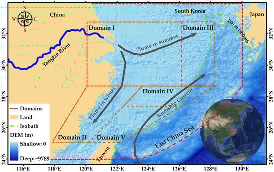
Figure 1.
The East China Sea and its partitions. The five domains indicated by red dashed lines are as defined by Guo et al. (2015). The green dashed line indicates a 200 m isobath. The areas of Domains I–V and the ECS are 20.23, 5.94, 9.56, 6.49, 5.90, and 63.92 × 10⁴ km2, respectively.
Excluding the Kuroshio domain, the sea surface temperature (SST) exhibits a northeast (low) to southwest (high) gradient year round. The summer–fall SST reaches 20–25 °C over the ECS shelf and ~28 °C out of the shelf, with a pronounced seasonal thermocline at a 15–30 m depth. The spring shelf SST falls below 15 °C, while the Kuroshio area remains at ~24 °C. In winter, the area with a low SST (<15 °C) shrinks relative to spring, yet the northern nearshore SST can plunge below 10 °C. The Chl-a concentration in the ECS shelf exceeds 3 μg/L, far surpassing that out of the shelf (<0.3 μg/L). The nearshore Chl-a peaks in summer due to the input of nutrients from the Changjiang plume, yet shows winter minima. However, elevated nutrient entrainment from deeper mixed layers sustains the maximum Chl-a in the outer shelf in winter. Additionally, the northeastward extension of high Chl-a water on the shelf in summer follows the Changjiang plume path. In contrast, the plume retreats in winter, and the biomass maxima expand southeastwards from the Subei Shallow.
According to different physical–biogeochemical characteristics based on the distributions of the SST, Chl-a, and turbidity [16], we divided the ECS shelf into five domains (Figure 1). Domain I includes the Changjiang estuary and the Changjiang plume in warm seasons, situated on the inner shelf with a depth of <50 m and distinguished by high Chl-a [26]. Domain II refers to the coastal ocean of Zhejiang–Fujian Province, China, with turbid coastal waters and the presence of the Changjiang plume in winter. Domains III, IV, and V are all located on the middle and outer shelf and are influenced by the Kuroshio, resulting in the characteristics of low nutrients and warm temperatures. Domain III is located on the northern ECS shelf, where the carbonate component is typically dominated by thermodynamics and the far-field Changjiang plume during flood seasons. Domain IV is located on the middle ECS shelf, marked by low Chl-a throughout different seasons and impacted by the Kuroshio; yet, it remains unaffected by the river plume [27]. Domain V is located on the southern ECS shelf, with its pCO2 levels determined by temperature and sometimes influenced by the upwelling of northern Taiwan [16].
2.2. Daily River-Monitoring Data
Following Dai et al. [28], we adopted the water discharge output into the ESC to indicate the seasonal changes in the terrestrial drought in the Changjiang River basin in 2022. Along the Yangtze River mainstream, the Datong hydrological station is the last gauge station (~600 km to the ECS), and its water level is unaffected by the ebb and flow of the ECS [15]. We obtained daily water level data at the Datong station during the period of 2003–2022 from the national water and rain information website, the Ministry of Water Resources of the People’s Republic of China (http://xxfb.mwr.cn/, accessed on 8 October 2023). On a daily scale, the arithmetic mean value during the period of 2003–2021 was calculated and compared with that in 2022.
2.3. Multi-Source Remote Sensing Products
The adopted monthly SST data with a 0.25-degree resolution (version 2.1) was the AVHRR_OI (optimal interpolation) dataset provided by the Group for High Resolution Sea Surface Temperature (GHRSST, https://www.ncei.noaa.gov/products/optimum-interpolation-sst, accessed on 16 July 2023), NOAA. The monthly sea surface Chl-a values employed in this study were derived from MODIS/Aqua with a spatial resolution of 4 km (version 2018.0, https://oceancolor.gsfc.nasa.gov/, accessed on 10 July 2023).
To obtain the seawater pCO2 and sea–air CO2 flux in the ECS, the remote sensing reflectance at 443 nm (Rrs(443), sr−1), 488 nm (Rrs(488)), and 555 nm (Rrs(555)), sea surface salinity (SSS, psu), wind speed at 10 m (WS, m/s), sea level pressure (SLP, m), and the mole fraction of CO2 in the dry air (xCO2) were used. The remote sensing reflectance was also derived from MODIS/Aqua (https://oceancolor.gsfc.nasa.gov/, accessed on 10 July 2023). The SSS was obtained from the GLOBAL-REANALYSIS-PHY-015-013 product of the Copernicus Marine Service (CMEMS), which has a spatial resolution of 0.083 degrees. Monthly SLP and xCO2 data with a spatial grid of 3° × 2° were obtained from CarbonTracker, NOAA (https://gml.noaa.gov/ccgg/carbontracker/, version CT2022B, accessed on 23 July 2023). WS data with a spatial resolution of 25 km and a temporal resolution of 1 month and 6 h were derived from the ECMWF Reanalysis v5 (ERA5) dataset provided by the European Centre for Medium-Range Weather Forecasts (ECMWF, https://www.ecmwf.int/en/forecasts/dataset/ecmwf-reanalysis-v5, accessed on 2 August 2023).
2.4. Remote CO2 Flux Calculation
To obtain seawater pCO2 (, μatm) in the ECS, a satellite algorithm called MeSAA-ML-ECS (Equation (1)) was adopted from the work of Yu et al. [18]. This algorithm combines the principles of a semi-mechanistic algorithm, MeSAA, and machine learning model, XGBoost. The input parameters consisted of three parts: (1) thermodynamics and forcing of increasing atmospheric CO2, represented by SST and thermodynamic pCO2; (2) mixing effect, represented by a proxy, , derived from SST; and (3) biological effects and other factors, represented by Chl-a and Rrs. for each pixel was calculated as the SST at that point minus the mean SST at the same latitude within the study area (117–135°E). The thermodynamic pCO2 () was calculated from the atmospheric pCO2 (, μatm) and SST using Equation (2).
where and are the yearly mean and SST (°C), respectively, and refers to the vapor pressure of water at 100% relative humidity. was gridded to 1 km when calculated from xCO2.
The seawater pCO2 data utilized in this study for the period of 2003 to 2019 were obtained from the open access dataset created by Yu et al. [18] (https://doi.org/10.5281/zenodo.8042265, accessed on 19 August 2023). The reliability of the satellite-derived seawater pCO2 was verified using measured data from Tsao et al. [29] at the intersection of the “PN line” and Kuroshio on the outer shelf of the ECS during the period of 2010 to 2018 (Figure S1). Thus, the seawater pCO2 in the ECS for the years 2020–2022 was also derived using the MeSAA-ML-ECS method.
Subsequent to obtaining the seawater pCO2 values, the sea–air CO2 flux (mmol/m2/day) between the surface water and the atmosphere was calculated using Equations (3)–(6) [16,18]. Finally, to assess the amount of carbon absorbed or released, the integrated CO2 flux (Tg C) was computed by multiplying the mean sea–air CO2 flux (mmol/m2/day) across the available pixels by the total area of the region and the total duration of the study period. Positive values of sea–air CO2 flux indicate CO2 release into the atmosphere, while negative values denote CO2 uptake by the sea.
where k is the gas transfer velocity; is the solubility of CO2 gas in seawater; and ΔpCO2 is the difference between the atmospheric and surface seawater pCO2 ().
where SST is the sea surface temperature in Kelvin, A1 = −60.2409, A2 = 93.4517, A_3 = 23.3585, B1 = 0.023517, B2 = −0.023656, and B3 = 0.0047036 [16].
where is the monthly mean WS; is the Schmidt number; is the nonlinear coefficient for the quadratic term of the gas transfer relationship; is the 6-hourly wind speed; the “mean” subscript indicates the average values; and n is the number of available wind speed measurements for each month.
2.5. Reference CO2 Uptake
Yu et al. [18] reported significant trends in the seawater pCO2 and sea–air CO2 flux in the ECS during the period of 2003–2019. The overall rise in the seawater pCO2 in the ECS was 0.78 μatm/yr. The continental shelf did not show a significant increase, but the Changjiang plume area and the area beyond the shelf displayed increases of 3–4 μatm/yr and ~1 μatm/yr, respectively. This indicates that the carbon sink in the ECS has improved, except for the Changjiang plume and the northern region beyond the continental shelf. However, the sea–air CO2 flux decreased at a rate of 0.3–0.4 mmol/m2/d per year in the continental shelf south of 30°N. Overall, the annual integrated CO2 uptake of the ECS increased from 10 Tg C in 2003 to 19 Tg C in 2019, with an increasing trend of 0.73 Tg C/yr.
In this study, the reference seawater pCO2 and CO2 fluxes were calculated based on the climatological monthly data and annual trends reported by Yu et al. [18], to illustrate the theoretical pCO2 and sea–air CO2 fluxes without the influence of MHW and terrestrial drought in 2022. Figure S2 shows specific trend maps with respect to the seawater pCO2 and sea–air CO2 flux. In the calculations, insignificant trends are considered as zero. For instance, the reference seawater pCO2 in July 2022 would be calculated using the mean pCO2 in July of 2003–2021 plus the reported annual trends (μatm/yr) multiplied by the number of years. In this case, the number of years is 11 (years since the middle of the period 2003–2021, i.e., 2012).
2.6. Contributors to the Seawater pCO2 Change
To quantify the drivers of seawater pCO2 change in 2022, we calculated the contributions of temperature-dependent thermodynamic and biological effects to the seawater pCO2 change.
The thermodynamic effect on pCO2 has an empirical relationship of approximately 4.23%/1 °C [30,31,32], which can be expressed as per Equation (2) in Section 2.4. In Equation (2), is the reference seawater pCO2, and SST and are the sea surface temperature in 2022 and the climatological SST (2003–2021 mean, in °C), respectively. That is to say, we calculated the change in pCO2 caused by the SST in 2022 compared to the absence of heat waves (SST anomalies).
Similarly, we used an empirical equation to estimate the biological effects on the seawater pCO2 change. Bai et al. [11] derived a regression equation (Equation (7)) for the biological effect in the ECS via a proxy of satellite-derived Chl-a (). The values corresponding to Chl-a in 2022 and climatological Chl-a (2003–2021 mean) were calculated, and the difference was regarded as the contribution of the biological effect to the pCO2 changes in 2022.
3. Results
3.1. Heatwave and Drought Events in 2022
Figure 2 depicts the 2022 values and the corresponding climatological mean (2003–2021) values of the daily water level at Datong Hydrological Station in the Changjiang River and the monthly mean SST for Domain I. Being relative to the multi-year mean, the SST in Domain I exceeded the baseline by over 1 °C in the period of January-April and July-August 2022, peaking in July 2022. Specifically, the SST in July 2022 reached 28.07 °C, which was 2.19 °C higher than the climatological averages in July. The SST in the period November-December 2022 was also elevated by 0.8 °C over the climatological means.
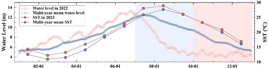
Figure 2.
Water level for the Changjiang River and mean SST for the Changjiang plume. The blue box covers July–September and the red box covers October–December.
The Changjiang discharge modestly exceeded the climatological averages (2003–2021) during the first half of 2022, peaking in June (Figure 2). However, an abrupt decline ensued in July–August. At the Datong station, water levels plunged from 12.7 m to 9.0 m in July, markedly below the multi-year July averages (>12 m). The reduction in the water level slowed down after August 10th, stabilizing around 5.8 m by the end of August and at 4.7 m (50%) under the climatological mean. Then, a reduced discharge lingered around 4–5 m until the end of 2022. These results indicate that the drought event in the Changjiang River began in July and continued until the end of 2022. Accordingly, we examined the July-September and October-December periods to elucidate the spatiotemporal characteristics of the seawater pCO2 and sea–air CO2 flux changes in the ECS under the compounding MHW and terrestrial drought events, especially the changes in the Changjiang plume area (Domain I in Figure 1).
3.2. Changes in pCO2 in 2022
In July-September 2022, the reference pCO2 was considerably higher in the Changjiang estuary and coastal area than that in the offshore waters. Moreover, the region affected by the Changjiang plume exhibited the lowest pCO2, and the outer shelf displayed an intermediate value of pCO2 (Figure 3c). Across the domains, on average, the lowest pCO2 could be found in Domains I and III, which were affected by the Changjiang River plume, with mean pCO2 values of 370 and 372 μatm, respectively. Meanwhile, the pCO2 values in the three southern domains (Domains II, IV, and V) were high and close to each other, ranging from 381 to 388 μatm. The whole ECS had an average pCO2 value of 383 μatm (Figure 4). From October to December 2022, the reference pCO2 in the Changjiang River estuary and coastal region decreased but was still high compared to other areas. Additionally, the pCO2 in the shelf increased significantly, while the pCO2 in other regions decreased (Figure 4). The pCO2 values in Domains I and II, with mean values of 381 and 387 μatm, respectively, were significantly higher than those in Domains III-V. The domain with the lowest mean pCO2 was Domain IV (345 μatm). The overall reference mean pCO2 for the entire ECS in October-December 2022 was 367 μatm.
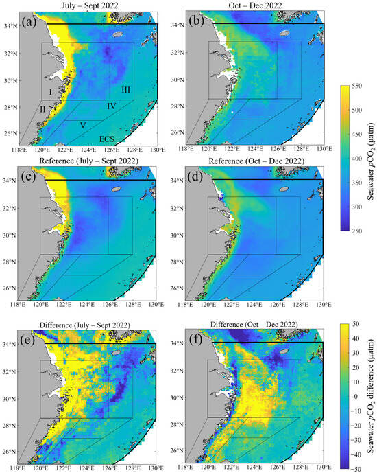
Figure 3.
Satellite-derived mean seawater pCO2 (a,b), reference seawater pCO2 (c,d), and differences between them (e,f) in July–Sept and Oct–Dec 2022. The seawater pCO2 difference was calculated by subtracting the reference pCO2 from the satellite-derived pCO2 in 2022. Specifically, the data in (e) are those in (a) minus those in (c), and the data in (f) are those in (b) minus those in (d).
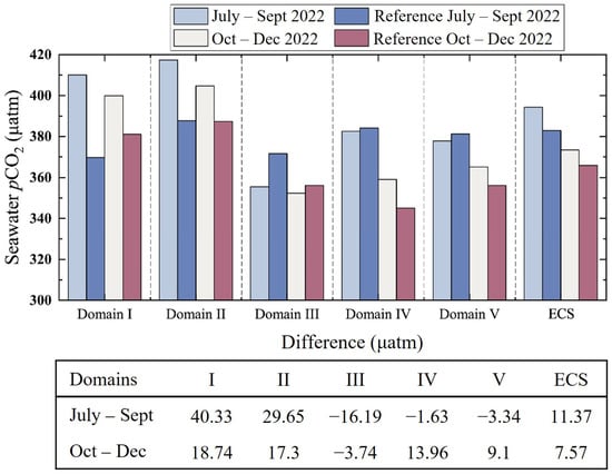
Figure 4.
Comparisons between regional means of the satellite-derived seawater pCO2 and the reference pCO2 during July–Sept and Oct–Dec 2022 in the five domains and the entire ECS. In the side table, the numbers show the differences between the satellite-derived and the reference seawater pCO2. Table S1 shows the exact values for each of the regions.
The actual spatial distribution of the pCO2 in the latter half of 2022 was comparable to its reference counterpart (Figure 3a–d). However, in July-September, the pCO2 was considerably elevated in the continental shelf affected by the Changjiang plume and in the coastal zone of Zhejiang and Fujian (Domains I and II, 410 and 417 μatm, respectively), compared to the reference values (Figure 3e and Figure 4). In the middle and outer shelf (Domain III), the pCO2 values were significantly lower than those in other regions (355 μatm). The regional average pCO2 in the whole ECS (394 μatm) was observed to be 11 μatm higher than the reference value (Figure 4). In October-December 2022, the pCO2 was also higher than the reference values in all domains except for Domain III, with the highest pCO2 in Domains I and II (400 and 405 μatm, respectively, Figure 3f). Overall, the average seawater pCO2 of the whole ECS in October-December was 373 μatm, which is 8 μatm higher than the reference value (Figure 4). That is to say, the compounding MHW and terrestrial drought event in 2022 resulted in a general pCO2 increase in the ECS.
3.3. Changes in CO2 Uptake in 2022
The sea–air CO2 flux pattern was similar to that of the seawater pCO2 (Figure 3 and Figure 5). Generally, a high seawater pCO2 (higher than atmospheric pCO2) indicates a positive sea–air CO2 flux, whereby seawater releases CO2 into the atmosphere, i.e., the ocean is a CO2 source, and the flux value increases with a higher pCO2. Conversely, a low seawater pCO2 corresponds to a negative CO2 flux, whereby seawater absorbs CO2 and acts as a CO2 sink.
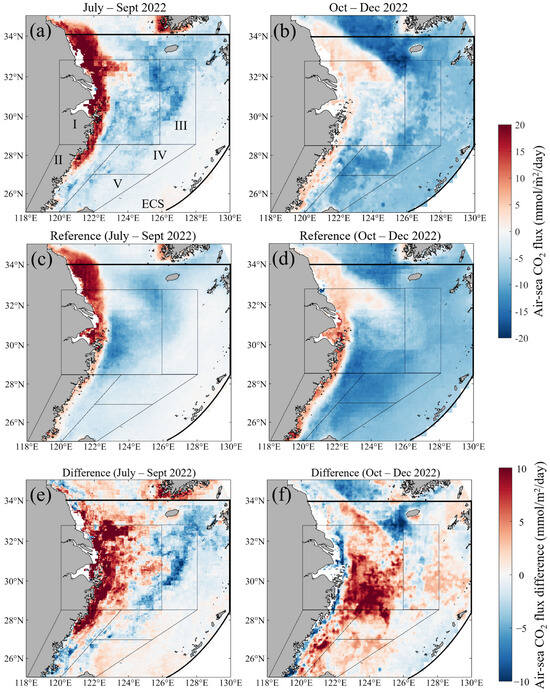
Figure 5.
Satellite-derived sea–air CO2 flux (a,b), reference sea–air CO2 flux (c,d), and differences between them (e,f) in July–Sept and Oct–Dec 2022. The sea–air CO2 flux difference was calculated using the reference CO2 flux from the satellite-derived CO2 flux in 2022. Specifically, the data in (e) are those in (a) minus those in (c), and the data in (f) are those in (b) minus those in (d).
The reference values of the sea–air CO2 flux indicate that the coastal region acted as a prominent CO2 source during July–September 2022, with an efflux of up to 20 mmol/m2/day (Figure 5c). In contrast, the Changjiang plume region acted as a stronger sink, with a flux of approximately −10–−15 mmol/m2/day. The remaining areas of the ECS indicated either a weak sink or were in source–sink equilibrium (Figure 5c). On average, the CO2 sink in Domain I (−3.21 mmol/m2/day) was the strongest among the five domains due to the large shelf area affected by the Changjiang River plume, which outweighed the effects of the near-shore regions (Figure 6). In comparison, Domains III–V had a weaker CO2 sink of −2.34–−2.95 mmol/m2/d, and Domain II had the weakest sink (−1.33 mmol/m2/day). The average CO2 flux across the ECS was −1.97 mmol/m2/day (Figure 6).
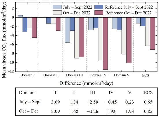
Figure 6.
Comparisons between the satellite-derived mean sea–air CO2 flux and the reference sea–air CO2 flux during July–Sept and Oct–Dec 2022 in the five domains and the entire ECS. In the side table, the numbers show the differences between the satellite-derived and the reference sea–air CO2 flux. Table S2 shows the exact values for each of the regions.
From October to December, the overall CO2 uptake in the ECS strengthened (Figure 5d). The near-shore area remained a source of atmospheric CO2, but the flux was less than 5 mmol/m2/day. The ECS shelf was the strongest CO2 sink, followed by the outer shelf. As the carbon-rich water extended southeastward from the Subei Shallow to Domain I, the reference mean CO2 influxes in Domain I and II (−3 and −5 mmol/m2/day) were much lower than those in Domains III–V (−9–−12 mmol/m2/day). The reference sea–air CO2 flux for the whole ECS in October-December 2022 averaged −7.15 mmol/m2/day, which is a stronger carbon sink compared to that in July-September of the same year (Figure 6).
The actual sea–air CO2 flux in the second half of 2022 was significantly lower compared to the reference values (Figure 5a,b), i.e., the CO2 uptake in the ECS weakened dramatically against the background of the MHW and drought events. In July-September, the CO2 flux near the shore was higher than the reference value by more than 10 mmol/m2/day (Figure 5a,e). Thus, the source–sink pattern of Domains I and II was reversed. Domain I became a source of atmospheric CO2 with an average CO2 flux of 0.48 mmol/m2/day (3.69 mmol/m2/day higher than the reference), and Domain II reached the state of source–sink equilibrium with a mean CO2 flux of 0.02 mmol/m2 /day (Figure 6). However, the shelf edge of Domain III exhibited significantly negative differences compared to the reference values, causing the regional mean CO2 uptake to almost double at a rate of −5.54 mmol/m2/day (Figure 5e and Figure 6). The mean CO2 uptake capacities of Domains IV and V were in line with the reference values, at rates of −2.79 and −2.56 mmol/m2/day, respectively (Figure 6).
During the months from October to December 2022, the sea–air CO2 flux differences between the satellite-derived and reference values on the ECS shelf were notably positive, except for the very near-shore water and the region to the southwest of Jeju Island, also indicating a weakened CO2 uptake. Specifically, the CO2 uptake capabilities of Domains I and II were found to be reduced by approximately 50%, resulting in values of −2.39 and −1.29 mmol/m2/day, respectively. Domains IV and V also exhibited 15–20% lower values, resulting in regional mean values of −9.63 and −8.16 mmol/m2/day, respectively. The mean flux in Domain III was consistent with the reference value. Overall, the actual sea–air CO2 flux in the entire ECS was −6.31 mmol/m2/day.
To quantify the direct influence of the MHW and terrestrial drought event in CO2 sinking in the second half of 2022, we calculated the integrated CO2 uptake fluxes for different domains and the entire ECS (Table 1). Domains I and II, which are directly affected by the Changjiang diluted water, showed the most significant changes in CO2 uptake. In July–September 2022, Domain I shifted from a projected carbon sink of 0.72 Tg C uptake to a source of 0.11 Tg C release, while Domain II reached source–sink equilibrium. In October–December, the carbon uptake of Domains I and II also decreased by half, with reference uptake values of 1.00 and 0.19 Tg C, and actual uptake values of only 0.53 and 0.08 Tg C, respectively. Comparatively speaking, the impacts of the MHW and terrestrial drought on Domains III–V were less severe. For Domains IV and V, the factual CO2 uptake values during the latter half of 2022 were 0.11 (11.0%) and 0.14 (16.7%) Tg C less when compared to the reference values. In contrast, in Domain III, there was an increase of 0.3 Tg C (24.2%) in the actual CO2 uptake during the latter half of 2022 compared to the reference amount, with nearly doubled uptake in July–September. Despite the expectation that the ECS would take up 6.44 Tg C of CO2 from the atmosphere during the second half of 2022, under the compounding MHW and terrestrial drought extreme events, only 5.38 Tg C was actually absorbed, with a reduction of 17.0%.

Table 1.
Integrated CO2 uptake (has the opposite sign to CO2 fluxes) for the five domains and the entire ECS in 2022.
4. Discussion
4.1. Driving Mechanism for the Changes in CO2 Uptake in 2022
Recent reports have indicated that the impact of MHWs on the sea–air CO2 flux is due to the combined effects of two competing mechanisms: (1) an increased sea surface temperature might reduce the solubility of CO2 in seawater, thus reducing CO2 uptake or enhancing CO2 release; and (2) enhanced density stratification might diminish vertical mixing and entrainment, lowering the dissolved inorganic carbon concentration (DIC) in the upper layer and increasing the CO2 uptake or decreasing CO2 release [5,33].
In July–September 2022, the SST over the ECS was generally higher than the climatological mean, especially in the summer Changjiang River plume (the northern parts of Domains I and II), with SST anomalies of up to +1.5–2 °C (Figure 7c). In October–December, the intensity of the MHW decreased, and positive SST anomalies (approximately +1 °C) occurred in the far-shore waters of the coast and Domains III–V (Figure 7d). Combining Figure 3e,f and Figure 7c,d, we believe that the substantial CO2 release increase and absorption decrease in 2022 are associated with positive SST anomalies over the ECS shelf.
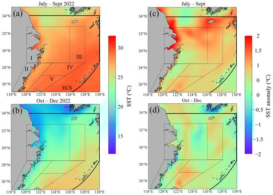
Figure 7.
SST (a,b) and SST anomaly (c,d) in Jul–Sept and Oct–Dec 2022. SST anomalies were calculated by subtracting the climatological mean SST (2003–2021) from the SST in 2022.
Another crucial factor contributing to CO2 uptake/release in the ECS is the biological process. The Changjiang diluted water brings abundant nutrients, which serve as essential inputs for phytoplankton growth in the ECS [34]. The intense terrestrial drought in 2022 caused a decrease of more than 50% in the Changjiang discharge into the ECS (Figure 1). This, in turn, is expected to lead to a decrease in the nutrient input. Figure 8 depicts the distribution of Chl-a in the ECS during the latter half of 2022, along with the difference between these values and the climatological mean results (Chl-a anomaly). Dramatic negative Chl-a anomalies (over −2 μg/L) were observed in the Changjiang plume in the period of July-September 2022 (Figure 8c). Similarly, Chl-a anomalies of −1–−1.5 μg/L occurred in the Changjiang River winter plume during October-December (Figure 8d). This reduction in phytoplankton biomass could potentially weaken the capacity of CO2 uptake here.
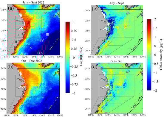
Figure 8.
Sea surface Chl-a (a,b) and Chl-a anomaly (c,d) in Jul–Sept and Oct–Dec 2022. Chl-a anomalies were calculated by subtracting the climatological mean Chl-a (2003–2021) from the Chl-a in 2022.
Figure 9 shows the contributions of the temperature-dependent thermodynamics and biological effects to the change in pCO2 in 2022. Overall, the temperature and Chl-a anomalies in 2022 contributed to the increase in the pCO2 and thus to a decrease in CO2 uptake. During July–September 2022, there were substantial influences on pCO2 changes of approximately 15 μatm due to positive SST anomalies (Figure 9a). In Domains I and II, where the pCO2 increased the most, the thermodynamic effects accounted for 44% and 37% of the increases, respectively. In comparison to the thermodynamic effects, biological processes had a relatively small influence, contributing to 33% and 16% of the pCO2 increment in Domains I and II, respectively, while providing almost no contribution in Domains III–V (Figure 9a). During October-December 2022, the effect of the SST on the pCO2 decreased as the intensity of the MHW reduced. In Domains I and II, the temperature only contributed 5 μatm, and in Domains III-V, it dropped to approximately 10 μatm (Figure 9b). In contrast, the importance of the role of biological effects in promoting pCO2 increased in Domains III–V, at 12, 11, and 5 μatm, respectively, and decreased in Domains I and II at 6 and 1 μatm (Figure 9b).
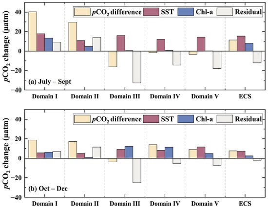
Figure 9.
Contributions of the SST and Chl-a to the seawater pCO2 difference (compared to the reference) in (a) Jul–Sept and (b) Oct–Dec 2022. Residuals were calculated by subtracting the SST and Chl-a contributions from the total pCO2 difference. Table S3 shows the exact values for each of the regions.
However, mixing effects might amplify and offset the positive contribution of thermodynamics and biological effects on the pCO2 in the inner and outer shelf, respectively. In the inner shelf, for Domains I and II, the residual contributes to 20–40% and 50–70% of the increase in pCO2, respectively. It is speculated that this increase may be due to a decrease in freshwater input caused by terrestrial drought, which weakens the stratification driven by plumes in the coastal area. The weakened stratification structure facilitates the return of sea-bottom waters with very high DIC to the surface, leading to an increase in surface pCO2 [35]. The mixing is typically more pronounced during the autumn and winter due to seasonal cooling and intensified monsoonal winds [35].
In contrast, in the outer shelf (Domain III–V), there was only a slight increase in pCO2, and even collective decreases in pCO2 were observed in July–September 2022. On the one hand, this may indicate that the competing balance of the MHW impact has tipped towards enhancing atmospheric CO2 uptake [5,33,36], consistent with Duke et al.’s [33] result in the northeast Pacific subpolar gyre. This could be due to enhanced density stratification resulting from high temperature, reducing vertical mixing and entrainment from subsurface water carrying high DIC [37,38]. On the other hand, it has been observed that the annual transport of DIC from the shelf to the ocean through the ‘Continental Shelf Pump’ (CSP) and physical pumping is approximately 70% of the inflow of inorganic carbon from rivers and the atmosphere, which balances the CO2 sink in the ECS shelf [37,38,39,40,41]. This massive cross-shelf exchange of inorganic carbon may effectively offset the increase in pCO2 contributed by the thermodynamics and biological effects.
In summary, the increase in CO2 release from seawater and the decrease in its absorption in the Changjiang River plume (Domain I and II) can be attributed to the combined effects of the MHW and terrestrial drought. However, the CO2 uptake on the outer shelf (Domains III–V) remained relatively constant or even increased, which may be due to complex physical and biogeochemical mechanisms.
4.2. Implications for CO2 Uptake in Global Marginal Seas
With continuous global warming, MHWs have become longer, more frequent, and stronger in the past century [42,43,44,45,46]. Notably, the frequency, duration, and intensity of MHWs in the ECS have been increasing in the past few years and are inspected to increase further in the future [47,48]. From 2016 to 2018, MHWs occurred during boreal summers in the ECS for three consecutive years, which was unprecedented in the past four decades according to the satellite record [49]. Subsequently, in the summer of 2022, the ECS continental shelf experienced one of the strongest and longest-lasting MHWs, breaking the previous record [50]. Additionally, terrestrial droughts are becoming more prevalent in river basins that flow into marginal seas and frequently co-occur with MHWs [51,52]. In 2022, the Changjiang diluted water discharge in August was recorded as the lowest since 1982 [50]. The co-occurrence of the MHW and terrestrial drought in 2022 resulted in a 17.0% (1.06 Tg C) reduction in CO2 uptake in the ECS, causing the Changjiang River plume region (Domain I) to shift from a CO2 sink to a source (releasing 0.11 Tg C) in July-September. The results of this study coincide with the findings of Mignot et al. [5] in the North Pacific subtropical gyre, where MHWs induced a reduction in CO2 uptake of 29 ± 11%. However, on the edge of the ECS shelf (Domain III), the MHW doubled the seawater CO2 sink in July–September 2022 (from 0.31 to 0.58 Tg). These results indicate that the impacts of MHWs on CO2 flux are intricate in the marginal sea, with significant spatial and temporal heterogeneity. It is necessary to conduct high-resolution regional research to better understand the effects of extreme weather and climate events on CO2 emission in marginal seas.
Additionally, previous studies have shown that MHWs often compound ocean acidity extremes, especially in the subtropics [53]. Ocean acidification may reduce the capability to take up atmospheric CO2 and further exacerbate global warming, creating a positive feedback effect. Therefore, extreme climate events (such as MHWs, ocean acidification, and droughts) and their impacts on the ocean carbon cycle should receive more attention in future studies.
5. Conclusions
Based on a variety of remote sensing products from multiple sources, we obtained seawater the pCO2 and sea–air CO2 flux values within the ESC from July to December 2022. Through comparisons with the reference values during the same period, we identified the spatial and temporal changes in CO2 uptake, considering the compounded effects of the extreme MHW and terrestrial drought events in 2022. Overall, the seawater pCO2 in the ECS was found to be generally higher than the reference value. Consequently, the absorption of CO2 decreased by 17% in the second half of 2022, when only 5.38 Tg C of CO2 was actually absorbed. In the majority of the ECS, the positive SST anomaly during the MHW diminished the solubility of CO2 in seawater, thereby reducing CO2 uptake. Additionally, the reduction in nutrient input associated with the terrestrial drought further reduced the capacity to take up CO2 due to unfavorable phytoplankton growth. In contrast, the CO2 uptake on the outer shelf remained constant or even increased. This research is important for comprehending the influences of extreme climatic events on CO2 uptake in marginal seas as well as the ambiguity in CO2 flux estimation under a complex climate warming scenario.
Supplementary Materials
The following supporting information can be downloaded at: https://www.mdpi.com/article/10.3390/rs16050849/s1, Figure S1: (a) the location of the “PN-line” (Tsao et al., 2023), (b) comparison between measured seawater pCO2 and time-series remote sensing data, and (c) comparison between measured seawater pCO2 and corresponding remote sensing data; Figure S2. Spatial distribution of trends during 2013–2019 in a) seawater pCO2, b) atmospheric pCO2, and c) air-sea CO2 flux, only pixels with significant trends are colored on the map (From Yu et al. (2023) Figure 7); Table S1: Partial pressure of CO2 (pCO2, μatm) for the five domains and the entire ECS in 2022; Table S2: Sea-air CO2 flux (mmol/m2/d) for the five domains and the entire ECS in 2022; Table S3: The contributions of SST and Chl-a to the seawater pCO2 difference for the five domains and the entire ECS in 2022; Table S4: Sea surface temperature (SST, °C) for the five domains and the entire ECS in 2022; Table S5: Chlorophyll-a concentration (Chl-a, μg/L) for the five domains and the entire ECS in 2022.
Author Contributions
Conceptualization, D.L.; data curation, Z.J., X.W. and X.D.; formal analysis, S.Y., Z.W. and T.L.; funding acquisition, T.L. and D.L.; methodology, S.Y. and Z.W.; software, X.D.; supervision, D.L.; validation, Z.J.; visualization, Z.W.; writing—original draft, S.Y.; writing—review and editing, S.Y., Z.W. and D.L. All authors have read and agreed to the published version of the manuscript.
Funding
This study was supported by the National Key Research and Development Program of China (Grants #2022YFF0801402 and #2023YFC3108102), the National Natural Science Foundation of China (Grants #42271376 and #41901299), the Natural Science Foundation of Jiangsu Province (Grant #BK20181102), the Youth Innovation Promotion Association CAS (Grant #2021313), the NIGLAS Foundation (Grant #E1SL002), and Research Project of China Three Gorges Corporation (Grant #202103552).
Data Availability Statement
Data will be made available upon request.
Conflicts of Interest
The authors declare no conflicts of interest.
References
- Roobaert, A.; Laruelle, G.G.; Landschützer, P.; Gruber, N.; Chou, L.; Regnier, P. The Spatiotemporal Dynamics of the Sources and Sinks of CO2 in the Global Coastal Ocean. Glob. Biogeochem. Cycles 2019, 33, 1693–1714. [Google Scholar] [CrossRef]
- Friedlingstein, P.; O’Sullivan, M.; Jones, M.W.; Andrew, R.M.; Gregor, L.; Hauck, J.; Le Quéré, C.; Luijkx, I.T.; Olsen, A.; Peters, G.P.; et al. Global Carbon Budget 2022. Earth Syst. Sci. Data 2022, 14, 4811–4900. [Google Scholar] [CrossRef]
- Laruelle, G.G.; Dürr, H.H.; Slomp, C.P.; Borges, A.V. Evaluation of sinks and sources of CO2 in the global coastal ocean using a spatially-explicit typology of estuaries and continental shelves. Geophys. Res. Lett. 2010, 37, L15607. [Google Scholar] [CrossRef]
- Borges, A.V. Do we have enough pieces of the jigsaw to integrate CO2 fluxes in the coastal ocean? Estuaries 2005, 28, 3–27. [Google Scholar] [CrossRef]
- Mignot, A.; von Schuckmann, K.; Landschutzer, P.; Gasparin, F.; van Gennip, S.; Perruche, C.; Lamouroux, J.; Amm, T. Decrease in air-sea CO2 fluxes caused by persistent marine heatwaves. Nat. Commun. 2022, 13, 4300. [Google Scholar] [CrossRef] [PubMed]
- Sharples, J.; Middelburg, J.J.; Fennel, K.; Jickells, T.D. What proportion of riverine nutrients reaches the open ocean? Glob. Biogeochem. Cycles 2017, 31, 39–58. [Google Scholar] [CrossRef]
- Regnier, P.; Resplandy, L.; Najjar, R.G.; Ciais, P. The land-to-ocean loops of the global carbon cycle. Nature 2022, 603, 401–410. [Google Scholar] [CrossRef]
- Bauer, J.E.; Cai, W.J.; Raymond, P.A.; Bianchi, T.S.; Hopkinson, C.S.; Regnier, P.A. The changing carbon cycle of the coastal ocean. Nature 2013, 504, 61–70. [Google Scholar] [CrossRef] [PubMed]
- Boyce, D.G.; Lewis, M.R.; Worm, B. Global phytoplankton decline over the past century. Nature 2010, 466, 591–596. [Google Scholar] [CrossRef]
- Sallee, J.B.; Pellichero, V.; Akhoudas, C.; Pauthenet, E.; Vignes, L.; Schmidtko, S.; Garabato, A.N.; Sutherland, P.; Kuusela, M. Summertime increases in upper-ocean stratification and mixed-layer depth. Nature 2021, 591, 592–598. [Google Scholar] [CrossRef]
- Bai, Y.; Cai, W.J.; He, X.; Zhai, W.; Pan, D.; Dai, M.; Yu, P. A mechanistic semi-analytical method for remotely sensing sea surface pCO2 in river-dominated coastal oceans: A case study from the East China Sea. J. Geophys. Res. Ocean. 2015, 120, 2331–2349. [Google Scholar] [CrossRef]
- Vicente-Serrano, S.M.; Quiring, S.M.; Peña-Gallardo, M.; Yuan, S.; Domínguez-Castro, F. A review of environmental droughts: Increased risk under global warming? Earth-Sci. Rev. 2020, 201, 102953. [Google Scholar] [CrossRef]
- Gao, G.; Zhao, X.; Jiang, M.; Gao, L. Impacts of Marine Heatwaves on Algal Structure and Carbon Sequestration in Conjunction With Ocean Warming and Acidification. Front. Mar. Sci. 2021, 8, 758651. [Google Scholar] [CrossRef]
- Wilbanks, K.A.; Sutter, L.A.; Amurao, J.M.; Batzer, D.P. Effects of drought on the physicochemical, nutrient, and carbon metrics of flows in the Savannah River, Georgia, USA. River Res. Appl. 2023, 39, 2048–2061. [Google Scholar] [CrossRef]
- Wang, X.; Ma, H.; Li, R.; Song, Z.; Wu, J. Seasonal fluxes and source variation of organic carbon transported by two major Chinese Rivers: The Yellow River and Changjiang (Yangtze) River. Glob. Biogeochem. Cycles 2012, 26, GB2025. [Google Scholar] [CrossRef]
- Guo, X.H.; Zhai, W.D.; Dai, M.H.; Zhang, C.; Bai, Y.; Xu, Y.; Li, Q.; Wang, G.Z. Air-sea CO2 fluxes in the East China Sea based on multiple-year underway observations. Biogeosciences 2015, 12, 5495–5514. [Google Scholar] [CrossRef]
- Liu, Q.; Guo, X.; Yin, Z.; Zhou, K.; Roberts, E.G.; Dai, M. Carbon fluxes in the China Seas: An overview and perspective. Sci. China Earth Sci. 2018, 61, 1564–1582. [Google Scholar] [CrossRef]
- Yu, S.; Song, Z.; Bai, Y.; Guo, X.; He, X.; Zhai, W.; Zhao, H.; Dai, M. Satellite-estimated air-sea CO2 fluxes in the Bohai Sea, Yellow Sea, and East China Sea: Patterns and variations during 2003–2019. Sci. Total. Environ. 2023, 904, 166804. [Google Scholar] [CrossRef]
- Liu, Y.; Yuan, S.; Zhu, Y.; Ren, L.; Chen, R.; Zhu, X.; Xia, R. The patterns, magnitude, and drivers of unprecedented 2022 mega-drought in the Yangtze River Basin, China. Environ. Res. Lett. 2023, 18, 114006. [Google Scholar] [CrossRef]
- Tan, H.-J.; Cai, R.-S.; Bai, D.-P.; Hilmi, K.; Tonbol, K. Causes of 2022 summer marine heatwave in the East China Seas. Adv. Clim. Chang. Res. 2023, 14, 633–641. [Google Scholar] [CrossRef]
- Guan, B. Winter Monsoon Counter-Currents in the Nearshore Waters off Southeastern China; China Ocean University Press: Qingdao, China, 2002. (In Chinese) [Google Scholar]
- Yuan, D.; Zhu, J.; Li, C.; Hu, D. Cross-shelf circulation in the Yellow and East China Seas indicated by MODIS satellite observations. J. Mar. Syst. 2008, 70, 134–149. [Google Scholar] [CrossRef]
- Dai, A.; Trenberth, K.E. Estimates of freshwater discharge from continents: Latitudinal and seasonal variations. J. Hydrometeorol. 2002, 3, 660–687. [Google Scholar] [CrossRef]
- Lee, H.-J.; Chao, S.-Y. A climatological description of circulation in and around the East China Sea. Deep. Sea Res. Part II Top. Stud. Oceanogr. 2003, 50, 1065–1084. [Google Scholar] [CrossRef]
- Zhu, J.; Shen, H. The Expansion Processes of the Changjiang River Diluted Water; East China Normal University Press: Shanghai, China, 1997. (In Chinese) [Google Scholar]
- He, X.; Bai, Y.; Pan, D.; Chen, C.-T.; Cheng, Q.; Wang, D.; Gong, F. Satellite views of the seasonal and interannual variability of phytoplankton blooms in the eastern China seas over the past 14 yr (1998–2011). Biogeosciences 2013, 10, 4721–4739. [Google Scholar] [CrossRef]
- Bai, Y.; He, X.; Pan, D.; Chen, C.T.A.; Kang, Y.; Chen, X.; Cai, W.J. Summertime Changjiang River plume variation during 1998–2010. J. Geophys. Res. Ocean. 2014, 119, 6238–6257. [Google Scholar] [CrossRef]
- Dai, Z.; Du, J.; Li, J.; Li, W.; Chen, J. Runoff characteristics of the Changjiang River during 2006: Effect of extreme drought and the impounding of the Three Gorges Dam. Geophys. Res. Lett. 2008, 35, L07406. [Google Scholar] [CrossRef]
- Tsao, S.E.; Shen, P.Y.; Tseng, C.M. Rapid increase of pCO2 and seawater acidification along Kuroshio at the east edge of the East China Sea. Mar. Pollut. Bull. 2023, 186, 114471. [Google Scholar] [CrossRef]
- Takahashi, T.; Olafsson, J.; Goddard, J.G.; Chipman, D.W.; Sutherland, S. Seasonal variation of CO2 and nutrients in the high-latitude surface oceans: A comparative study. Glob. Biogeochem. Cycles 1993, 7, 843–878. [Google Scholar] [CrossRef]
- Takahashi, T.; Sutherland, S.C.; Sweeney, C.; Poisson, A.; Metzl, N.; Tilbrook, B.; Bates, N.; Wanninkhof, R.; Feely, R.A.; Sabine, C. Global sea–air CO2 flux based on climatological surface ocean pCO2, and seasonal biological and temperature effects. Deep. Sea Res. Part II Top. Stud. Oceanogr. 2002, 49, 1601–1622. [Google Scholar] [CrossRef]
- Takahashi, T.; Sutherland, S.C.; Wanninkhof, R.; Sweeney, C.; Feely, R.A.; Chipman, D.W.; Hales, B.; Friederich, G.; Chavez, F.; Sabine, C. Climatological mean and decadal change in surface ocean pCO2, and net sea–air CO2 flux over the global oceans. Deep. Sea Res. Part II Top. Stud. Oceanogr. 2009, 56, 554–577. [Google Scholar] [CrossRef]
- Duke, P.J.; Hamme, R.C.; Ianson, D.; Landschützer, P.; Ahmed, M.M.; Swart, N.C.; Covert, P.A. Estimating Marine Carbon Uptake in the Northeast Pacific Using a Neural Network Approach. EGUsphere 2023, 2023, 1–38. [Google Scholar] [CrossRef]
- Wang, B.-D.; Wang, X.-L.; Zhan, R. Nutrient conditions in the yellow sea and the east china sea. Estuar. Coast. Shelf Sci. 2003, 58, 127–136. [Google Scholar] [CrossRef]
- Chou, W.C.; Gong, G.C.; Cai, W.J.; Tseng, C.M. Seasonality of CO2 in coastal oceans altered by increasing anthropogenic nutrient delivery from large rivers: Evidence from the Changjiang–East China Sea system. Biogeosciences 2013, 10, 3889–3899. [Google Scholar] [CrossRef]
- Edwing, K.; Wu, Z.; Lu, W.; Li, X.; Cai, W.J.; Yan, X.H. Impact of Marine Heatwaves on Air-Sea CO2 Flux along the US East Coast. Geophys. Res. Lett. 2024, 51, e2023GL105363. [Google Scholar] [CrossRef]
- Dai, M.; Su, J.; Zhao, Y.; Hofmann, E.E.; Cao, Z.; Cai, W.-J.; Gan, J.; Lacroix, F.; Laruelle, G.G.; Meng, F.; et al. Carbon Fluxes in the Coastal Ocean: Synthesis, Boundary Processes, and Future Trends. Annu. Rev. Earth Planet. Sci. 2022, 50, 593–626. [Google Scholar] [CrossRef]
- Fennel, K.; Alin, S.; Barbero, L.; Evans, W.; Bourgeois, T.; Cooley, S.; Dunne, J.; Feely, R.A.; Hernandez-Ayon, J.M.; Hu, X.; et al. Carbon cycling in the North American coastal ocean: A synthesis. Biogeosciences 2019, 16, 1281–1304. [Google Scholar] [CrossRef]
- Na, R.; Rong, Z.; Wang, Z.A.; Liang, S.; Liu, C.; Ringham, M.; Liang, H. Air-sea CO2 fluxes and cross-shelf exchange of inorganic carbon in the East China Sea from a coupled physical-biogeochemical model. Sci. Total. Environ. 2024, 906, 167572. [Google Scholar] [CrossRef] [PubMed]
- Najjar, R.G.; Herrmann, M.; Alexander, R.; Boyer, E.W.; Burdige, D.J.; Butman, D.; Cai, W.J.; Canuel, E.A.; Chen, R.F.; Friedrichs, M.A.M.; et al. Carbon Budget of Tidal Wetlands, Estuaries, and Shelf Waters of Eastern North America. Glob. Biogeochem. Cycles 2018, 32, 389–416. [Google Scholar] [CrossRef]
- Tsunogai, S.; Watanabe, S.; Sato, T. Is there a “continental shelf pump” for the absorption of atmospheric CO2? Tellus B Chem. Phys. Meteorol. 1999, 51, 701–712. [Google Scholar] [CrossRef]
- Frölicher, T.L.; Fischer, E.M.; Gruber, N. Marine heatwaves under global warming. Nature 2018, 560, 360–364. [Google Scholar] [CrossRef]
- Holbrook, N.J.; Scannell, H.A.; Sen Gupta, A.; Benthuysen, J.A.; Feng, M.; Oliver, E.C.; Alexander, L.V.; Burrows, M.T.; Donat, M.G.; Hobday, A.J. A global assessment of marine heatwaves and their drivers. Nat. Commun. 2019, 10, 2624. [Google Scholar] [CrossRef]
- Laufkötter, C.; Zscheischler, J.; Frölicher, T.L. High-impact marine heatwaves attributable to human-induced global warming. Science 2020, 369, 1621–1625. [Google Scholar] [CrossRef]
- Oliver, E.C.; Benthuysen, J.A.; Darmaraki, S.; Donat, M.G.; Hobday, A.J.; Holbrook, N.J.; Schlegel, R.W.; Sen Gupta, A. Marine heatwaves. Annu. Rev. Mar. Sci. 2021, 13, 313–342. [Google Scholar] [CrossRef]
- Oliver, E.C.; Donat, M.G.; Burrows, M.T.; Moore, P.J.; Smale, D.A.; Alexander, L.V.; Benthuysen, J.A.; Feng, M.; Sen Gupta, A.; Hobday, A.J. Longer and more frequent marine heatwaves over the past century. Nat. Commun. 2018, 9, 1324. [Google Scholar] [CrossRef]
- Tan, H.; Cai, R. What caused the record-breaking warming in East China Seas during August 2016? Atmos. Sci. Lett. 2018, 19, e853. [Google Scholar] [CrossRef]
- Yao, Y.; Wang, J.; Yin, J.; Zou, X. Marine heatwaves in China’s marginal seas and adjacent offshore waters: Past, present, and future. J. Geophys. Res. Ocean. 2020, 125, e2019JC015801. [Google Scholar] [CrossRef]
- Gao, G.; Marin, M.; Feng, M.; Yin, B.; Yang, D.; Feng, X.; Ding, Y.; Song, D. Drivers of marine heatwaves in the East China Sea and the South Yellow Sea in three consecutive summers during 2016–2018. J. Geophys. Res. Ocean. 2020, 125, e2020JC016518. [Google Scholar] [CrossRef]
- Oh, H.; Kim, G.-U.; Chu, J.-E.; Lee, K.; Jeong, J.-Y. The record-breaking 2022 long-lasting marine heatwaves in the East China Sea. Environ. Res. Lett. 2023, 18, 064015. [Google Scholar] [CrossRef]
- Rodrigues, R.R.; Taschetto, A.S.; Sen Gupta, A.; Foltz, G.R. Common cause for severe droughts in South America and marine heatwaves in the South Atlantic. Nat. Geosci. 2019, 12, 620–626. [Google Scholar] [CrossRef]
- Shi, H.; García-Reyes, M.; Jacox, M.G.; Rykaczewski, R.R.; Black, B.A.; Bograd, S.J.; Sydeman, W.J. Co-occurrence of California drought and Northeast Pacific marine heatwaves under climate change. Geophys. Res. Lett. 2021, 48, e2021GL092765. [Google Scholar] [CrossRef]
- Burger, F.A.; Terhaar, J.; Frölicher, T.L. Compound marine heatwaves and ocean acidity extremes. Nat. Commun. 2022, 13, 4722. [Google Scholar] [CrossRef] [PubMed]
Disclaimer/Publisher’s Note: The statements, opinions and data contained in all publications are solely those of the individual author(s) and contributor(s) and not of MDPI and/or the editor(s). MDPI and/or the editor(s) disclaim responsibility for any injury to people or property resulting from any ideas, methods, instructions or products referred to in the content. |
© 2024 by the authors. Licensee MDPI, Basel, Switzerland. This article is an open access article distributed under the terms and conditions of the Creative Commons Attribution (CC BY) license (https://creativecommons.org/licenses/by/4.0/).