
Mapping Remote Roads Using Artificial Intelligence and Satellite Imagery

 ,
,  , and
, and 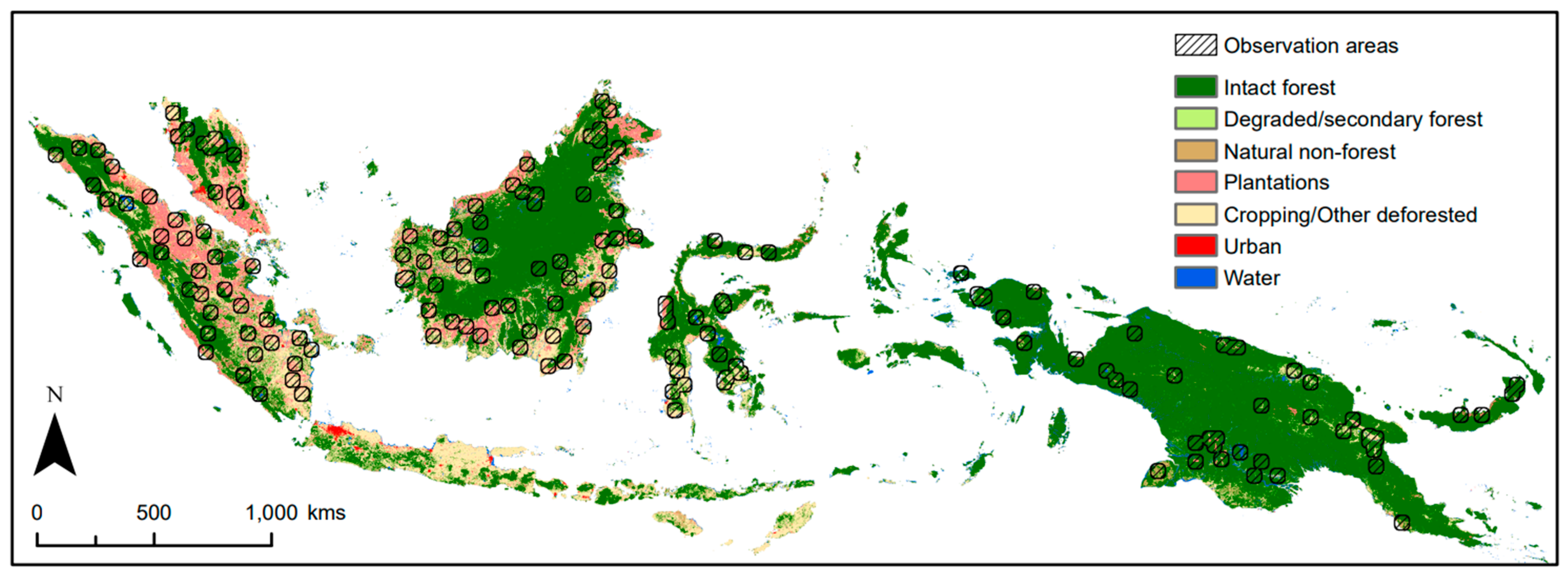
Abstract
1. Introduction
2. Materials and Methods
2.1. Overview
2.2. Satellite Imagery and Road Reference Data
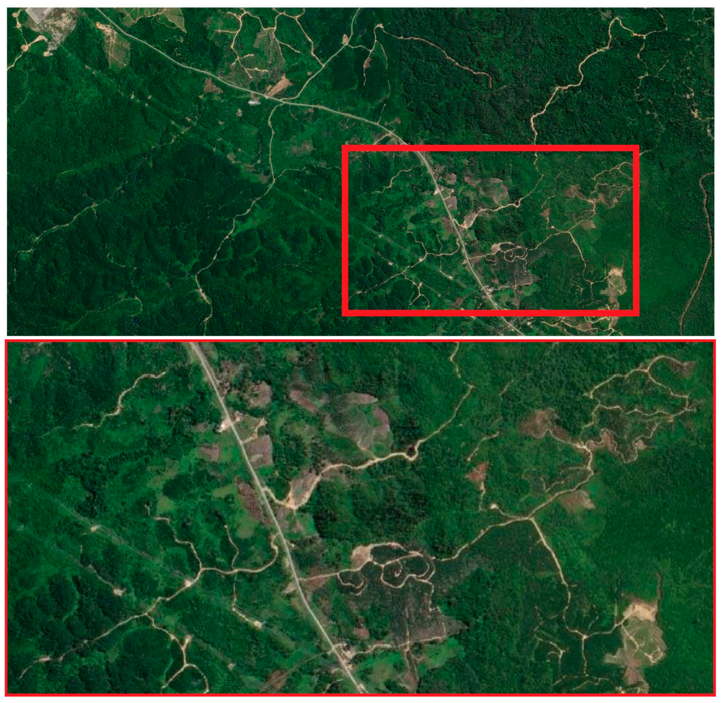
2.2.1. Study Area
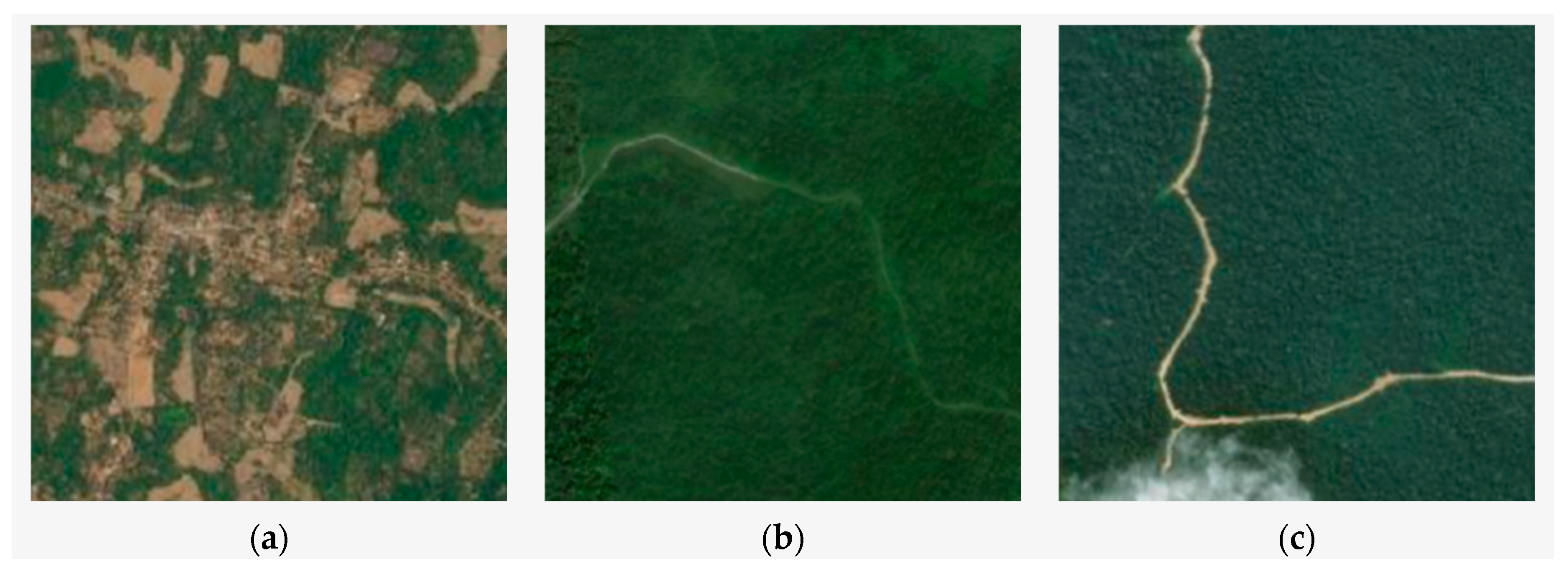
2.2.2. Satellite Imagery
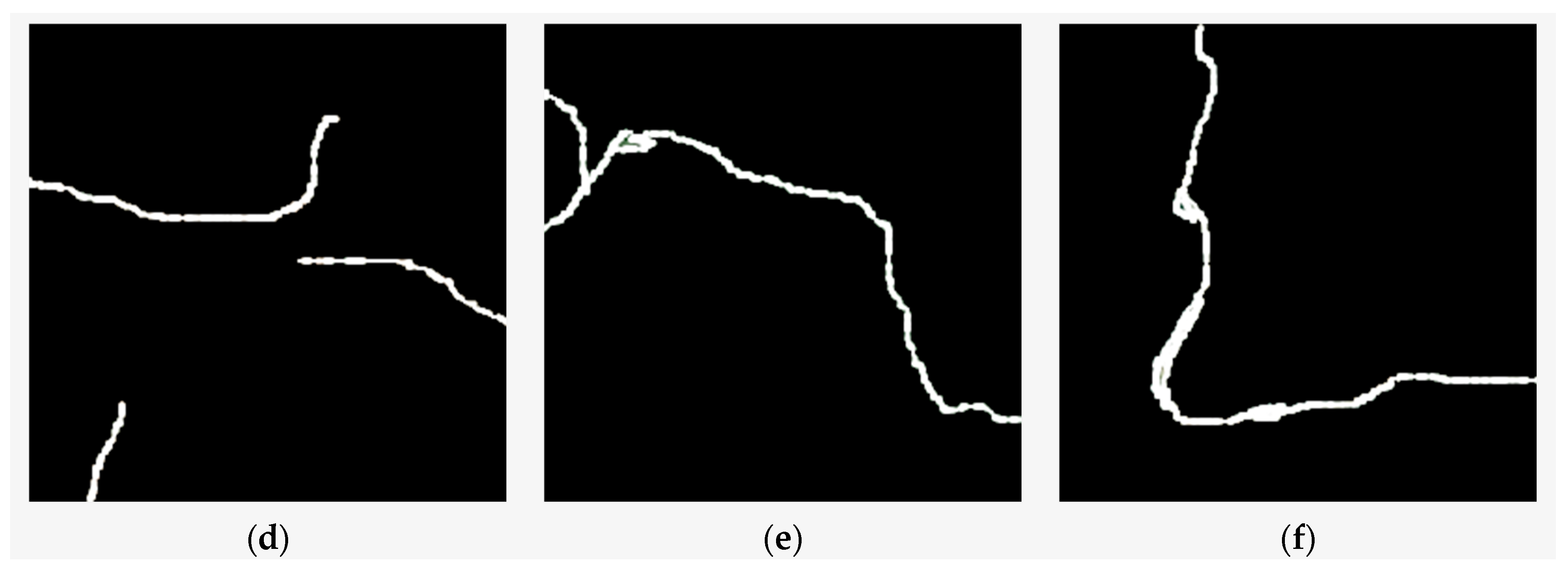
2.2.3. Road Reference Data
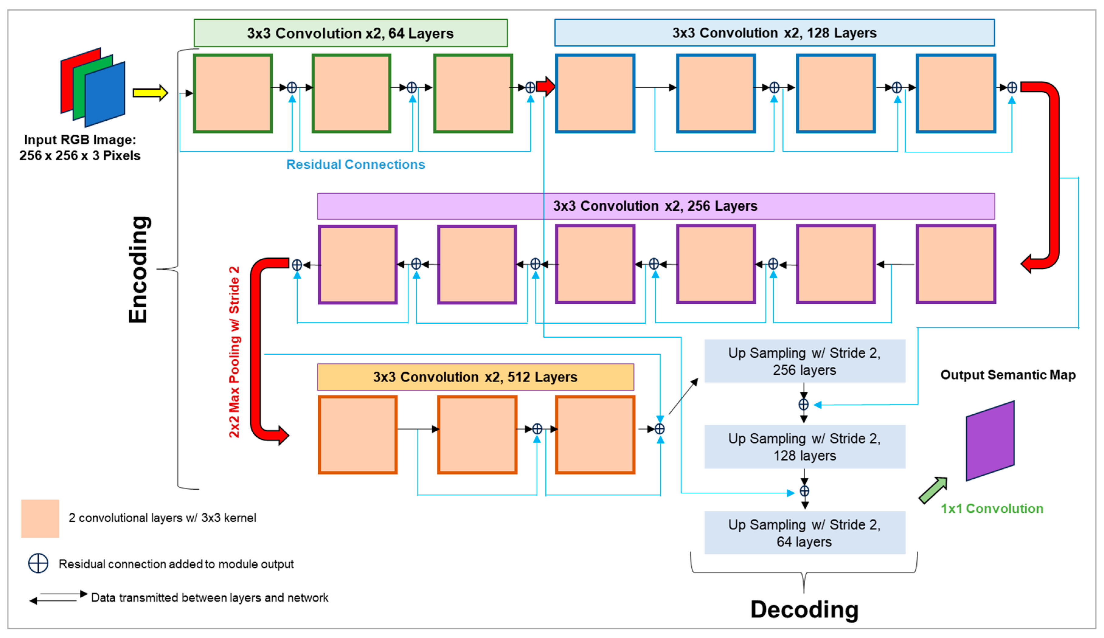
2.3. Machine Learning Models for Road Mapping
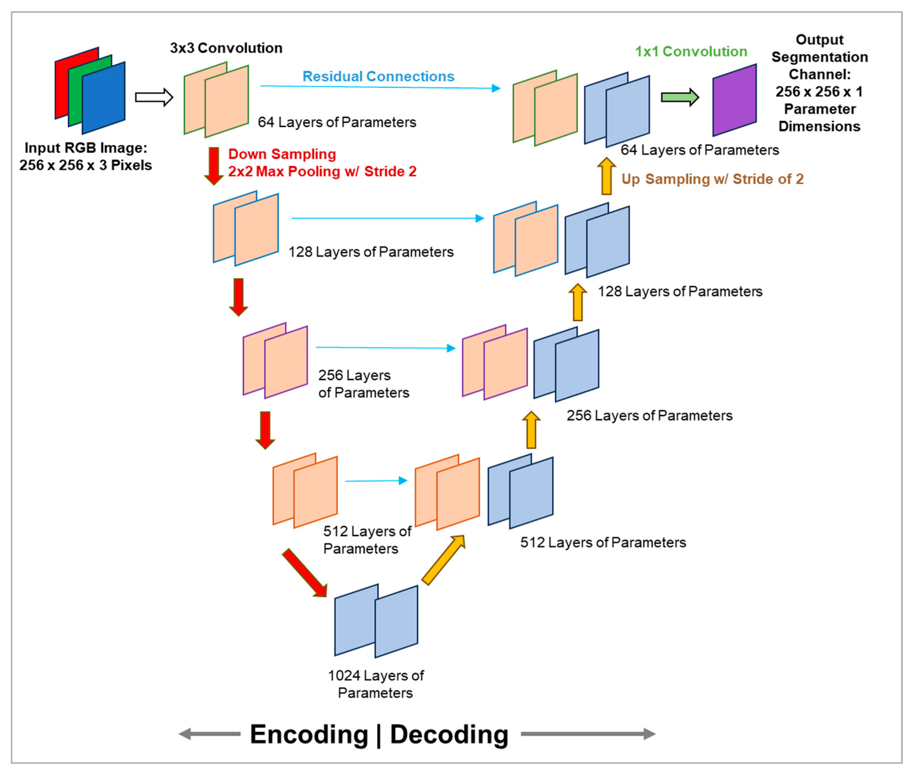
2.3.1. UNet Model
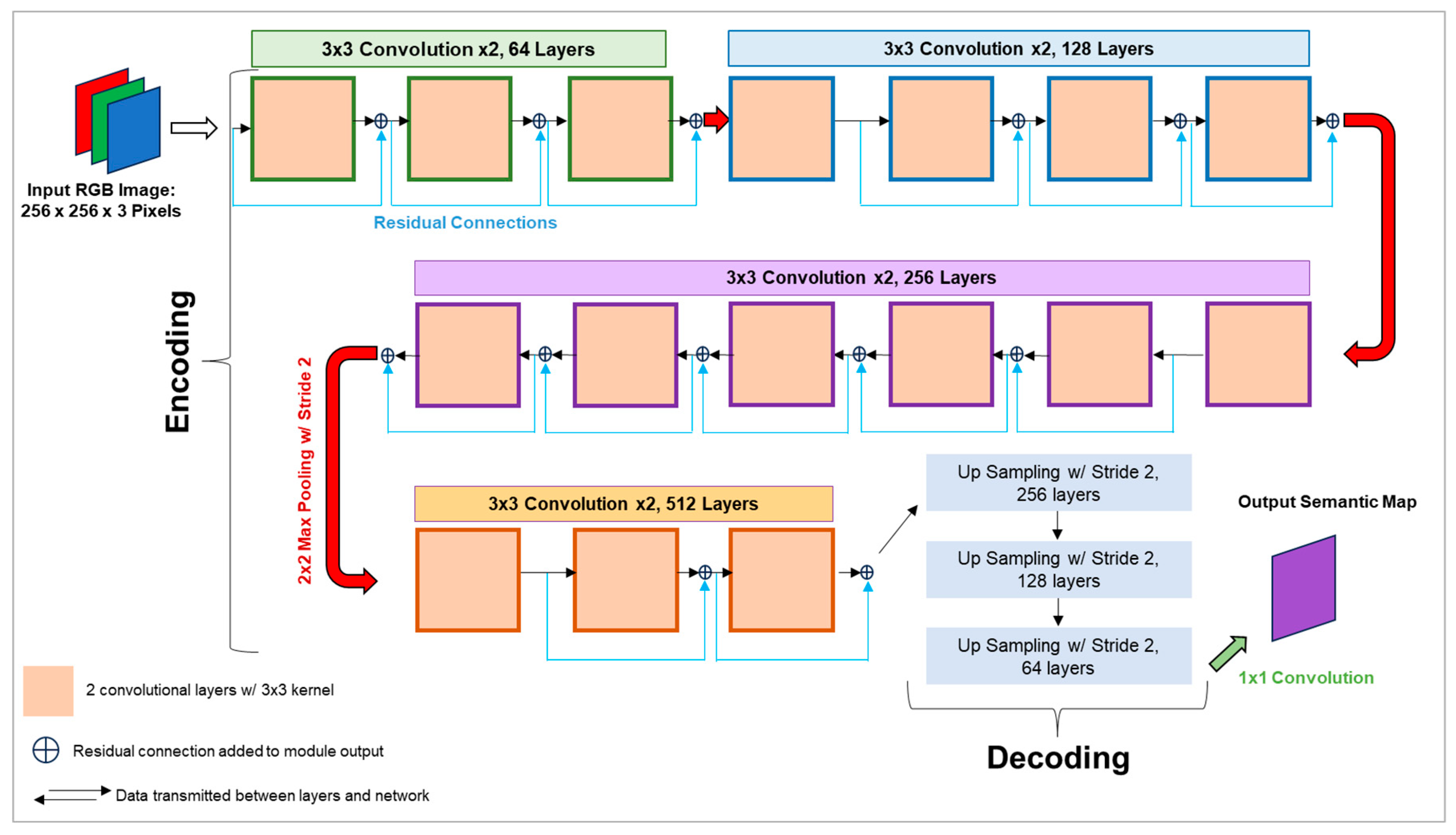
2.3.2. ResNet-34 Model
2.3.3. Resnet-34 Model with Added Residual Connections (ResNet-34+)
2.4. Model Training and Validation
2.5. Model Testing
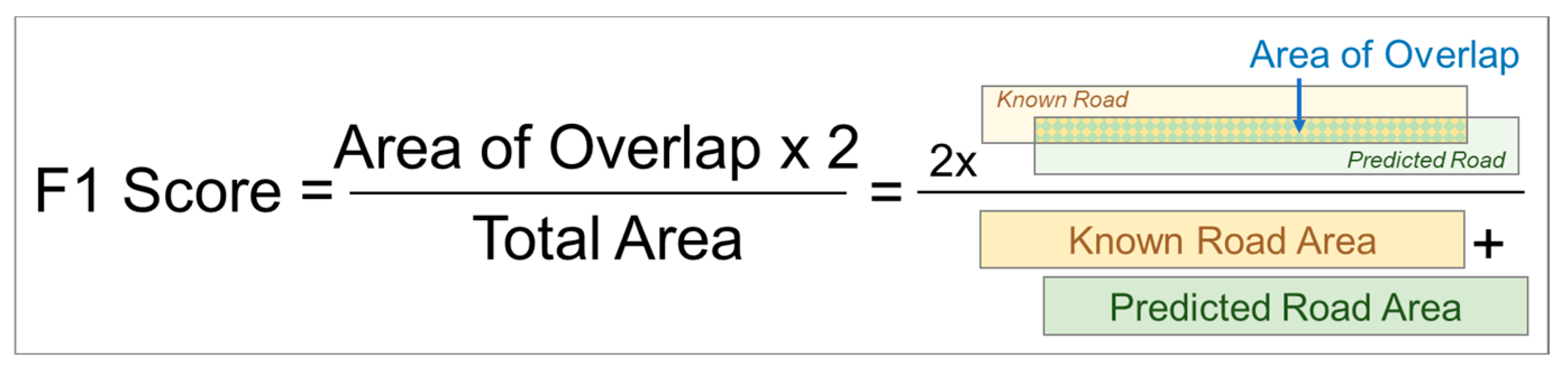
2.5.1. F1 Score of Model Accuracy
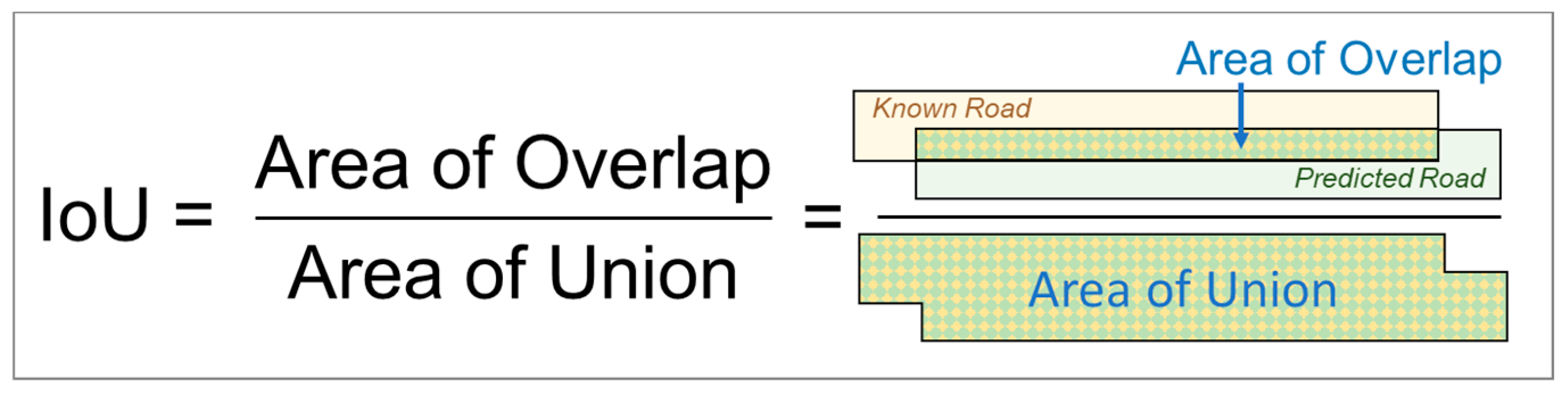
2.5.2. Mean Intersection over Union Metric of Model Accuracy
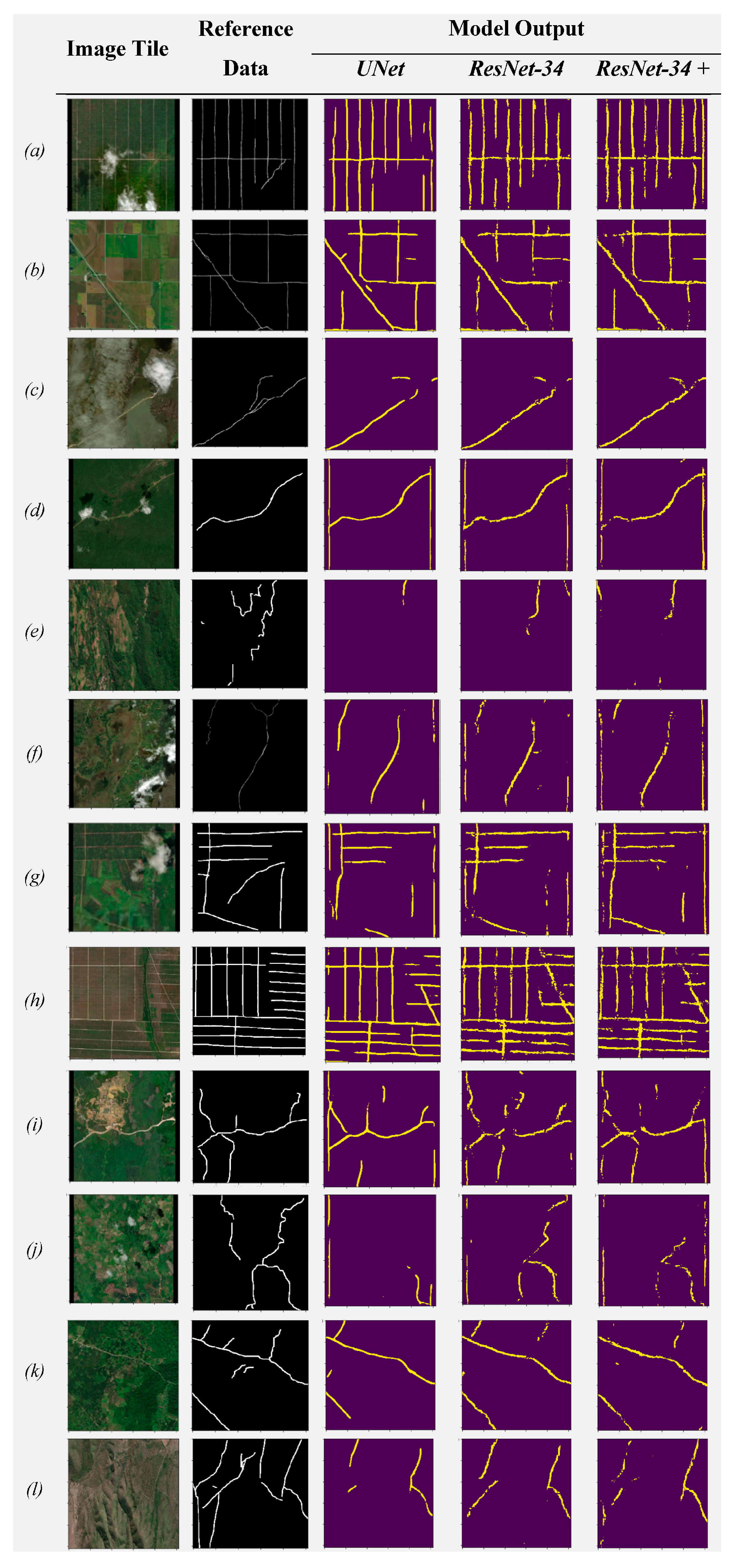
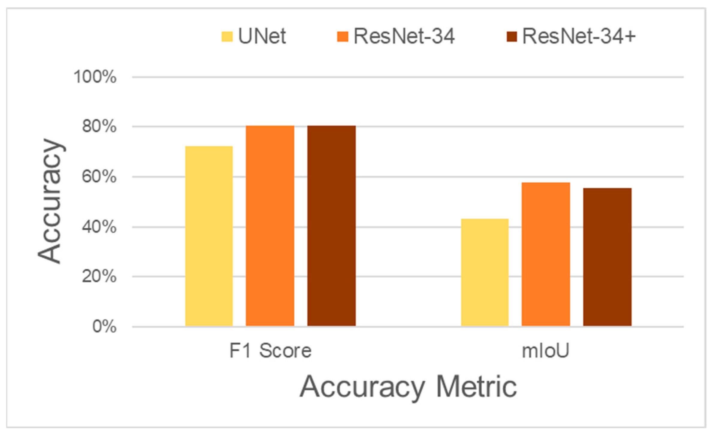
3. Results
4. Discussion
Supplementary Materials
Author Contributions
Funding
Data Availability Statement
Acknowledgments
Conflicts of Interest
| 1 | The term ‘human-curated road data’ implies data generated by human contributions to the OSM database and excludes road data generated by ML models. The following text notes Facebook Roads road data generated by an ML model and added to OSM. |
References
- Dulac, J. Global Land Transport Infrastructure Requirements: Estimating Road and Railway Infrastructure Capacity and Costs to 2050; International Energy Agency: Paris, France, 2013. [Google Scholar]
- Hettige, H. When Do Rural Roads Benefit the Poor and How? An In-Depth Analysis; Asian Development Bank: Manilla, Philippines, 2006. [Google Scholar]
- Laurance, W.F.; Goosem, M.; Laurance, S.G.W. Impacts of roads and linear clearings on tropical forests. Trends Ecol. Evol. 2009, 24, 659–669. [Google Scholar] [CrossRef]
- Ascensão, F.; Fahrig, L.; Clevenger, A.P.; Corlett, R.T.; Jaeger, J.A.G.; Laurance, W.F.; Pereira, H.M. Environmental challenges for the Belt and Road Initiative. Nat. Sustain. 2018, 1, 206–209. [Google Scholar] [CrossRef]
- Kleinschroth, F.; Laporte, N.; Laurance, W.F.; Goetz, S.; Ghazoul, J. Road expansion and persistence in forests of the Congo Basin. Nat. Sustain. 2019, 2, 628–634. [Google Scholar] [CrossRef]
- Ibisch, P.L.; Hoffmann, M.T.; Kreft, S.; Pe’er, G.; Kati, V.; Biber-Freudenberger, L.; DellaSala, D.A.; Vale, M.M.; Hobson, P.R.; Selva, N. A global map of roadless areas and their conservation status. Science 2016, 354, 1423–1427. [Google Scholar] [CrossRef]
- Laurance, W.F.; Cochrane, M.A.; Bergen, S.; Fearnside, P.M.; Delamônica, P.; Barber, C.; D’Angelo, S.; Fernandes, T. The Future of the Brazilian Amazon. Science 2001, 291, 438–439. [Google Scholar] [CrossRef]
- Wali, A. The transformation of a frontier: State and regional relationships in Panama, 1972–1990. Hum. Organ. 1993, 52, 115–129. [Google Scholar] [CrossRef]
- Pfaff, A.; Robalino, J.; Walker, R.; Aldrich, S.; Caldas, M.; Reis, E.; Perz, S.; Bohrer, C.; Arima, E.; Laurance, W.; et al. Road investments, spatial spillovers, and deforestation in the Brazilian Amazon. J. Reg. Sci. 2007, 47, 109–123. [Google Scholar] [CrossRef]
- Barber, C.P.; Cochrane, M.A.; Souza, C.M., Jr.; Laurance, W.F. Roads, deforestation, and the mitigating effect of protected areas in the Amazon. Biol. Conserv. 2014, 177, 203–209. [Google Scholar] [CrossRef]
- Hughes, A.C. Have Indo-Malaysian forests reached the end of the road? Biol. Conserv. 2018, 223, 129–137. [Google Scholar] [CrossRef]
- Souza, C.; Ribeiro, J.G.; Botelho, J.P.J.; Kirchhoff, F.T. Advances on Earth Observation and Artificial Intelligence to Map Unofficial Roads in the Brazilian Amazon Biome. Paper Presented at American Geophysical Union, Fall Meeting, 2020, December. Available online: https://ui.adsabs.harvard.edu/abs/2020AGUFMGC106..09S/abstract (accessed on 5 June 2023).
- Botelho, J.; Costa, S.C.P.; Ribeiro, J.G.; Souza, C.M. Mapping roads in the Brazilian Amazon with artificial intelligence and Sentinel-2. Remote Sens. 2022, 14, 3625. [Google Scholar] [CrossRef]
- Meijer, J.R.; Huijbregts, M.A.J.; Schotten, K.C.G.J.; Schipper, A.M. Global patterns of current and future road infrastructure. Environ. Res. Lett. 2018, 13, 064006. [Google Scholar] [CrossRef]
- Das Neves, P.B.T.; Blanco, C.J.C.; Montenegro Duarte, A.A.A.; das Neves, F.B.S.; das Neves, I.B.S.; de Paula dos Santos, M.H. Amazon rainforest deforestation influenced by clandestine and regular roadway network. Land Use Policy 2021, 108, 105510. [Google Scholar] [CrossRef]
- Engert, J.; Campbell, M.J.; Cinner, J.; Ishida, Y.; Sloan, S.; Alamgir, M.; Cislowski, J.; Laurance, W.F. ‘Ghost roads’ and the survival of tropical forests. Nature 2024. [Google Scholar]
- Engert, J.E.; Ishida, F.Y.; Laurance, W.F. Rerouting a major Indonesian mining road to spare nature and reduce development costs. Conserv. Sci. Pract. 2021, 3, e521. [Google Scholar] [CrossRef]
- BBC. Facebook Uses AI to Map Thailand’s Roads. BBC News. 24 July 2019. Available online: https://www.bbc.com/news/technology-49091093 (accessed on 2 January 2023).
- Cole, L.J. Mapping the World. Pegasus: The Magazine of the University of Central Florida. 2020. Available online: https://www.ucf.edu/pegasus/mapping-the-world/ (accessed on 2 June 2023).
- Sloan, S.; Campbell, M.J.; Alamgir, M.; Collier-Baker, E.; Nowak, M.; Usher, G.; Laurance, W.F. Infrastructure development and contested forest governance threaten the Leuser Ecosystem, Indonesia. Land Use Policy 2018, 77, 298–309. [Google Scholar] [CrossRef]
- Brandão, A.O.; Souza, C.M. Mapping unofficial roads with Landsat images: A new tool to improve the monitoring of the Brazilian Amazon rainforest. Int. J. Remote Sens. 2006, 27, 177–189. [Google Scholar] [CrossRef]
- Laporte, N.T.; Stabach, J.A.; Grosch, R.; Lin, T.S.; Goetz, S.J. Expansion of industrial logging in Central Africa. Science 2007, 316, 1451. [Google Scholar] [CrossRef]
- Gaveau, D.L.A.; Sloan, S.; Molidena, M.; Yaen, H.; Sheil, D.; Abram, N.K.; Ancrenaz, M.; Nasi, R.; Quinones, M.; Wielaard, N.; et al. Four Decades of Forest Persistence, Clearance and Logging on Borneo. PLoS ONE 2014, 9, e101654. [Google Scholar] [CrossRef] [PubMed]
- Sloan, S.; Alamgir, M.; Campbell, M.J.; Setyawati, T.; Laurance, W.F. Development Corridors and Remnant-Forest Conservation in Sumatra, Indonesia. Trop. Conserv. Sci. 2019, 12, 194008291988950. [Google Scholar] [CrossRef]
- Laurance, W.F.; Achard, F.; Peedell, S.; Schmitt, S. Big data, big opportunities. Front. Ecol. Environ. 2016, 14, 347. [Google Scholar] [CrossRef]
- Abdollahi, A.; Pradhan, B.; Shukla, N.; Chakraborty, S.; Alamri, A. Deep learning approaches applied to remote sensing datasets for road extraction: A state-of-the-art review. Remote Sens. 2020, 12, 1444. [Google Scholar] [CrossRef]
- Gabriele Moser, J.Z. Mathematical Models for Remote Sensing Image Processing; Springer: Berlin/Heidelberg, Germany, 2018. [Google Scholar]
- Yuan, X.; Shi, J.; Gu, L. A review of deep learning methods for semantic segmentation of remote sensing imagery. Expert Syst. Appl. 2021, 169, 114417. [Google Scholar] [CrossRef]
- Hoeser, T.; Kuenzer, C. Object detection and image segmentation with deep learning on Earth observation data: A review—Part I: Evolution and recent trends. Remote Sens. 2020, 12, 1667. [Google Scholar] [CrossRef]
- Diakogiannis, F.I.; Waldner, F.; Caccetta, P.; Wu, C. ResUNet-a: A deep learning framework for semantic segmentation of remotely sensed data. ISPRS J. Photogramm. Remote Sens. 2020, 162, 94–114. [Google Scholar] [CrossRef]
- Alshehhi, R.; Marpu, P.R.; Woon, W.L.; Mura, M.D. Simultaneous extraction of roads and buildings in remote sensing imagery with convolutional neural networks. ISPRS J. Photogramm. Remote Sens. 2017, 130, 139–149. [Google Scholar] [CrossRef]
- Gao, L.; Song, W.; Dai, J.; Chen, Y. Road extraction from high-resolution remote sensing imagery using refined deep residual convolutional neural network. Remote Sens. 2019, 11, 552. [Google Scholar] [CrossRef]
- Buslaev, A.; Seferbekov, S.; Iglovikov, V.; Shvets, A. Fully Convolutional Network for Automatic Road Extraction from Satellite Imagery. In Proceedings of the 2018 IEEE/CVF Conference on Computer Vision and Pattern Recognition Workshops (CVPRW), Salt Lake City, UT, USA, 18–22 June 2018; pp. 207–210. [Google Scholar]
- Liu, J.; Qin, Q.; Li, J.; Li, Y. Rural road extraction from high-resolution remote sensing images based on geometric feature inference. ISPRS Int. J. Geo-Inf. 2017, 6, 314. [Google Scholar] [CrossRef]
- Dai, J.; Ma, R.; Ai, H. Semi-automatic extraction of rural roads from high-resolution remote sensing images based on a multifeature combination. IEEE Geosci. Remote Sens. Lett. 2022, 19, 3000605. [Google Scholar] [CrossRef]
- Bonafilia, D.; Gill, J.; Basu, S.; Yang, D. Building high resolution maps for humanitarian aid and development with weakly- and semi-supervised learning. In Proceedings of the IEEE/CVF Conference on Computer Vision and Pattern Recognition (CVPR) Workshops, Long Beach, CA, USA, 15–20 June 2019; pp. 1–9. [Google Scholar]
- Facebook. Open Mapping at Facebook—A Documentation Repository and Data Host for Facebook’s Mapping-with-AI Project on OpenStreetMap. Available online: https://github.com/facebookmicrosites/Open-Mapping-At-Facebook (accessed on 2 August 2023).
- Wurm, M.; Stark, T.; Zhu, X.X.; Weigand, M.; Taubenböck, H. Semantic segmentation of slums in satellite images using transfer learning on fully convolutional neural networks. ISPRS J. Photogramm. Remote Sens. 2019, 150, 59–69. [Google Scholar] [CrossRef]
- He, K.; Zhang, X.; Ren, S.; Sun, J. Deep residual learning for image recognition. In Proceedings of the IEEE Conference on Computer Vision and Pattern Recognition (CVPR), Las Vegas, NV, USA, 27–30 June 2016; pp. 770–778. Available online: https://ieeexplore.ieee.org/document/7780459 (accessed on 5 August 2023).
- Alamgir, M.; Sloan, S.; Campbell, M.J.; Laurance, W.F. Regional economic growth initiative challenges sustainable development and forest conservation in Sarawak, Borneo. PLoS ONE 2020, 15, e0229614. [Google Scholar] [CrossRef]
- Alamgir, M.; Sloan, S.; Campbell, M.J.; Engert, J.; Laurance, W.F. Infrastructure expansion projects undermine sustainable development and forest conservation in Papua New Guinea. PLoS ONE 2019, 4, e0219408. [Google Scholar] [CrossRef]
- Alamgir, M.; Campbell, M.J.; Sloan, S.; Suhardiman, A.; Laurance, W.F. High-risk infrastructure projects pose imminent threats to forests in Indonesian Borneo. Sci. Rep. 2019, 9, 140. [Google Scholar] [CrossRef]
- Sloan, S.; Campbell, M.J.; Alamgir, M.; Lechner, A.M.; Engert, J.; Laurance, W.F. Trans-national conservation and infrastructure development in the Heart of Borneo. PLoS ONE 2019, 19, e0221947. [Google Scholar] [CrossRef]
- Sloan, S.; Campbell, M.; Alamgir, M.; Engert, J.; Ishida, F.Y.; Senn, N.; Huther, J.; Laurance, W.F. Hidden challenges for conservation and development along the Papuan economic corridor. Environ. Sci. Policy 2019, 92, 98–106. [Google Scholar] [CrossRef]
- Sloan, S.; Talkhani, R.R.; Huang, T.; Engert, J.; Laurance, W.F. Satellite Images and Road-Reference Images for AI-Based Road Mapping in Equatorial Asia. Datadryad.org. 2023. Available online: https://datadryad.org/stash/dataset/doi:10.5061/dryad.bvq83bkg7 (accessed on 5 August 2023). [CrossRef]
- Shorten, C.; Khoshgoftaar, T.M. A survey on image data augmentation for deep learning. J. Big Data 2019, 6, 60. [Google Scholar] [CrossRef]
- Ronneberger, O.; Fischer, P.; Brox, T. U-Net: Convolutional networks for biomedical image segmentation. arXiv 2015. [Google Scholar] [CrossRef]
- Li, Z.; Liu, F.; Yang, W.; Peng, S.; Zhou, J. A survey of convolutional neural networks: Analysis, applications, and prospects. IEEE Trans. Neural Netw. Learn. Syst. 2022, 33, 6999–7019. [Google Scholar] [CrossRef]
- Lin, Y.; Xu, D.; Wang, N.; Shi, Z.; Chen, Q. Road extraction from very-high-resolution remote sensing images via a nested SE-deeplab model. Remote Sens. 2020, 12, 2985. [Google Scholar] [CrossRef]
- Demir, I.; Koperski, K.; Lindenbaum, D.; Pang, G.; Huang, J.; Basu, S.; Hughes, F.; Tuia, D.; Raskar, R. Deepglobe 2018: A challenge to parse the earth through satellite images. In Proceedings of the IEEE Conference on Computer Vision and Pattern Recognition Workshops, Salt Lake City, UT, USA, 18–22 June 2018; pp. 172–181. [Google Scholar]
- Henry, C.; Azimi, S.M.; Merkle, N. Road segmentation in SAR satellite images with deep fully convolutional neural networks. IEEE Geosci. Remote Sens. Lett. 2018, 15, 1867–1871. [Google Scholar] [CrossRef]
- He, H.; Yang, D.; Wang, S.; Wang, S.; Liu, X. Road segmentation of cross-modal remote sensing images using deep segmentation network and transfer learning. Ind. Robot. Int. J. Robot. Res. Appl. 2019, 46, 384–390. [Google Scholar] [CrossRef]
- Doshi, J. Residual inception skip network for binary segmentation. In Proceedings of the IEEE Conference on Computer Vision and Pattern Recognition Workshops, Salt Lake City, UT, USA, 18–22 June 2018; pp. 216–219. [Google Scholar]
- Li, Y.; Xu, L.; Rao, J.; Guo, L.; Yan, Z.; Jin, S. A Y-Net deep learning method for road segmentation using high-resolution visible remote sensing images. Remote Sens. 2019, 10, 381–390. [Google Scholar] [CrossRef]
- Xie, Y.; Miao, F.; Zhou, K.; Peng, J. HsgNet: A road extraction network based on global perception of high-order spatial information. ISPRS Int. J. Geo-Inf. 2019, 8, 571. [Google Scholar] [CrossRef]
- Xin, J.; Zhang, X.; Zhang, Z.; Fang, W. Road extraction of high-resolution remote sensing images derived from DenseUNet. Remote Sens. 2019, 11, 2499. [Google Scholar] [CrossRef]
- Zhou, L.; Zhang, C.; Wu, M. D-LinkNet: LinkNet with pretrained encoder and dilated convolution for high resolution satellite imagery road extraction. In Proceedings of the IEEE Conference on Computer Vision and Pattern Recognition Workshops, Salt Lake City, UT, USA, 18–22 June 2018; pp. 182–186. [Google Scholar]
- Draper, C.; Adiatma, D.; Kanyenye, T.J. Reaching Inaccessible Communities Through Road Mapping for Sustainable Development. Available online: https://www.hotosm.org/updates/reaching-inaccessible-communities-through-road-mapping-for-sustainable-development/ (accessed on 3 February 2024).
- Máttyus, G.; Luo, W.; Urtasun, R. Deeproadmapper: Extracting road topology from aerial images. In Proceedings of the IEEE International Conference on Computer Vision, Venice, Italy, 22–29 October 2017; pp. 3438–3446. [Google Scholar]
- Zhang, Z.; Liu, Q.; Wang, Y. Road extraction by deep residual U-Net. IEEE Geosci. Andremote Sens. Lett. 2018, 15, 749–753. [Google Scholar] [CrossRef]
- Xu, Y.; Xie, Z.; Feng, Y.; Chen, Z. Road extraction from high-resolution remote sensing imagery using deep learning. Remote Sens. 2018, 10, 1461. [Google Scholar] [CrossRef]
- Sun, T.; Chen, Z.; Yang, W.; Wang, Y. Stacked U-Nets with multi-output for road extraction. In Proceedings of the IEEE/CVF Conference on Computer Vision and Pattern Recognition Workshops, Salt Lake City, UT, USA, 18–22 June 2018; pp. 202–206. [Google Scholar]
- Das, P.; Chand, S. Extracting road maps from high-resolution satellite imagery using refined DSE-LinkNet. Connect. Sci. 2021, 33, 278–295. [Google Scholar] [CrossRef]
- CVPR. DeepGlobe Road Extraction Challenge > Results. Available online: https://competitions.codalab.org/competitions/18467#results (accessed on 10 August 2023).
- Venter, O.; Sanderson, E.W.; Magrach, A.; Allan, J.R.; Beher, J.; Jones, K.R.; Possingham, H.P.; Laurance, W.F.; Wood, P.; Fekete, B.M.; et al. Sixteen years of change in the global terrestrial human footprint and implications for biodiversity conservation. Nat. Commun. 2016, 7, 12558. [Google Scholar] [CrossRef]
- Sanderson, E.W.; Jaiteh, M.; Levy, M.A.; Redford, K.H.; Wannebo, A.V.; Woolmer, G. The human footprint and the last of the wild. BioScience 2002, 52, 891–904. [Google Scholar] [CrossRef]
- Potapov, P.; Yaroshenko, A.; Turubanova, S.; Dubinin, M.; Laestadius, L.; Thies, C.; Aksenov, D.; Egorov, A.; Yesipova, Y.; Glushkov, I.; et al. Mapping the world’s intact forest landscapes by remote sensing. Ecol. Soc. 2008, 13, 51. [Google Scholar] [CrossRef]
- Sloan, S.; Jenkins, C.N.; Joppa, L.N.; Gaveau, D.L.A.; Laurance, W.F. Remaining natural vegetation in the global biodiversity hotspots. Biol. Conserv. 2014, 117, 12–24. [Google Scholar] [CrossRef]
- Hansen, M.C.; Krylov, A.; Tyukavina, A.; Potapov, P.V.; Turubanova, S.; Zutta, B.; Ifo, S.; Margono, B.; Stolle, F.; Moore, R. Humid tropical forest disturbance alerts using Landsat data. Environ. Res. Lett. 2016, 11, 034008. [Google Scholar] [CrossRef]
- Shang, R.; Zhu, Z.; Zhang, J.; Qiu, S.; Yang, Z.; Li, T.; Yang, X. Near-real-time monitoring of land disturbance with harmonized Landsats 7–8 and Sentinel-2 data. Remote Sens. Environ. 2022, 278, 113073. [Google Scholar] [CrossRef]
- Reymondin, L.; Jarvis, A.; Perez-Uribe, A.; Touval, J.; Argote, K.; Coca, A.; Rebetez, J.; Guevara, E.; Mulligan, M. A Methodology for Near Real-Time Monitoring of Habitat Change at Continental Scales Using MODIS-NDVI and TRMM; Terra-i & the International Centre for Tropical Agriculture (CIAT): Rome, Italy, 2012. [Google Scholar]
- Hansen, M.C.; Potapov, P.V.; Moore, R.; Hancher, M.; Turubanova, S.A.; Tyukavina, A.; Thau, D.; Stehman, S.V.; Goetz, S.J.; Loveland, T.R.; et al. High-resolution global maps of 21st-century forest cover change. Science 2013, 342, 850–853. [Google Scholar] [CrossRef]
- Justice, C.O.; Giglio, L.; Korontzi, S.; Owens, J.; Morisette, J.T.; Roy, D.; Descloitres, J.; Alleaume, S.; Petitcolin, F.; Kaufman, Y. The MODIS fire products. Remote Sens. Environ. 2002, 83, 244–262. [Google Scholar] [CrossRef]
- Sloan, S.; Locatelli, B.; Wooster, M.J.; Gaveau, D.L.A. Fire activity in Borneo driven by industrial land conversion and drought during El Niño periods, 1982–2010. Glob. Environ. Change 2017, 47, 95–109. [Google Scholar] [CrossRef]
- Sloan, S.; Tacconi, L.; Cattau, M.E. Fire prevention in managed landscapes: Recent successes and challenges in Indonesia. Mitig. Adapt. Strateg. Glob. Change 2021, 26, 32. [Google Scholar] [CrossRef]
- Sloan, S.; Locatelli, B.; Andela, N.; Cattau, M.; Gaveau, D.L.A.; Tacconi, L. Declining severe fire activity on managed lands in Equatorial Asia. Commun. Earth Environ. 2022, 3, 207. [Google Scholar] [CrossRef]
- Mittermeier, R.A.; Mittermeier, C.G.; Brooks, T.M.; Pilgrim, J.D.; Konstant, W.R.; da Fonseca, G.A.B.; Kormos, C. Wilderness and biodiversity conservation. Proc. Natl. Acad. Sci. USA 2003, 100, 10309–10313. [Google Scholar] [CrossRef]
- Fagan, M.E.; Kim, D.-H.; Settle, W.; Ferry, L.; Drew, J.; Carlson, H.; Slaughter, J.; Schaferbien, J.; Tyukavina, A.; Harris, N.; et al. The expansion of tree plantations across tropical biomes. Nat. Sustain. 2022, 5, 661–688. [Google Scholar] [CrossRef]
- Descals, A.; Wich, S.; Meijaard, E.; Gaveau, D.L.A.; Peedell, S.; Szantoi, Z. High-resolution global map of smallholder and industrial closed-canopy oil palm plantations. Earth Syst. Sci. Data 2021, 13, 1211–1231. [Google Scholar] [CrossRef]
- Harris, N.; Goldman Dow, E.; Gibbes, S. Spatial Database of Planted Trees (SPT Version 1.0), Technical Note; World Resources Institute: Washington, DC, USA, 2019; p. 36. [Google Scholar]
- Sloan, S.; Meyfroidt, P.; Rudel, T.K.; Bongers, F.; Chazdon Robin, L. The forest transformation: Planted tree cover and regional dynamics of tree gains and losses. Glob. Environ. Change 2019, 59, 101988. [Google Scholar] [CrossRef]
- Pesaresi, M.; Ehrlich, D.; Ferri, S.; Florczyk, A.J.; Freire, S.; Halkia, S.; Julea, A.M.; Kemper, T.; Soille, P.; Syrris, V. Operating Procedure for the Production of the Global Human Settlement Layer from Landsat Data of the Epochs 1975, 1990, 2000, and 2014; Publications Office of the European Union: Luxembourg, 2016. [Google Scholar]
- Reddiar, I.B.; Osti, M. Quantifying transportation infrastructure pressure on Southeast Asian World Heritage forests. Biol. Conserv. 2022, 270, 109564. [Google Scholar] [CrossRef]
- Neis, P.; Zielstra, D. Recent developments and future trends in volunteered geographic information research: The case of OpenStreetMap. Future Internet 2014, 6, 76–106. [Google Scholar] [CrossRef]
- Bey, A.; Sánchez-Paus Díaz, A.; Maniatis, D.; Marchi, G.; Mollicone, D.; Ricci, S.; Bastin, J.-F.; Moore, R.; Federici, S.; Rezende, M.; et al. Collect Earth: Land use and land cover assessment through augmented visual interpretation. Remote Sens. 2016, 8, 807. [Google Scholar] [CrossRef]
- Krietzberg, I. Big Tech Giants Are Working to Change the Mapping Industry. In TheStreet; The Arena Group: New York, NY, USA, 2023. [Google Scholar]
- Facebook. Open Mapping at Facebook—Map with AI Self-Service Training Document. Available online: https://github.com/facebookmicrosites/Open-Mapping-At-Facebook/wiki (accessed on 5 August 2023).
- KaartGroup. Java OpenStreetMap (JOSM) Map-with-AI PlugIn. Available online: https://github.com/KaartGroup/JOSM_MapWIthAI_plugin (accessed on 5 August 2023).
- Facebook. RapID (v.2)—An Online Interface for Editing OpenStreetMap, including Facebook Roads Data. Available online: https://rapideditor.org/ (accessed on 6 August 2023).


Disclaimer/Publisher’s Note: The statements, opinions and data contained in all publications are solely those of the individual author(s) and contributor(s) and not of MDPI and/or the editor(s). MDPI and/or the editor(s) disclaim responsibility for any injury to people or property resulting from any ideas, methods, instructions or products referred to in the content. |
© 2024 by the authors. Licensee MDPI, Basel, Switzerland. This article is an open access article distributed under the terms and conditions of the Creative Commons Attribution (CC BY) license (https://creativecommons.org/licenses/by/4.0/).
Share and Cite
Sloan, S.; Talkhani, R.R.; Huang, T.; Engert, J.; Laurance, W.F. Mapping Remote Roads Using Artificial Intelligence and Satellite Imagery. Remote Sens. 2024, 16, 839. https://doi.org/10.3390/rs16050839
Sloan S, Talkhani RR, Huang T, Engert J, Laurance WF. Mapping Remote Roads Using Artificial Intelligence and Satellite Imagery. Remote Sensing. 2024; 16(5):839. https://doi.org/10.3390/rs16050839
Chicago/Turabian StyleSloan, Sean, Raiyan R. Talkhani, Tao Huang, Jayden Engert, and William F. Laurance. 2024. "Mapping Remote Roads Using Artificial Intelligence and Satellite Imagery" Remote Sensing 16, no. 5: 839. https://doi.org/10.3390/rs16050839
APA StyleSloan, S., Talkhani, R. R., Huang, T., Engert, J., & Laurance, W. F. (2024). Mapping Remote Roads Using Artificial Intelligence and Satellite Imagery. Remote Sensing, 16(5), 839. https://doi.org/10.3390/rs16050839