Abstract
Unravelling slow ecosystem migration patterns requires a fundamental understanding of the broad-scale climatic drivers, which are further modulated by fine-scale heterogeneities just outside established ecosystem boundaries. While modern Unoccupied Aerial Vehicle (UAV) remote sensing approaches enable us to monitor local scale ecotone dynamics in unprecedented detail, they are often underutilised as a temporal snapshot of the conditions on site. In this study in the Southern Alps of New Zealand, we demonstrate how the combination of multispectral and thermal data, as well as LiDAR data (2019), supplemented by three decades (1991–2021) of treeline transect data can add great value to field monitoring campaigns by putting seedling regeneration patterns at treeline into a spatially explicit context. Orthorectification and mosaicking of RGB and multispectral imagery produced spatially extensive maps of the subalpine area (~4 ha) with low spatial offset (Craigieburn: 6.14 ± 4.03 cm; Mt Faust: 5.11 ± 2.88 cm, mean ± standard error). The seven multispectral bands enabled a highly detailed delineation of six ground cover classes at treeline. Subalpine shrubs were detected with high accuracy (up to 90%), and a clear identification of the closed forest canopy (Fuscospora cliffortioides, >95%) was achieved. Two thermal imaging flights revealed the effect of existing vegetation classes on ground-level thermal conditions. UAV LiDAR data acquisition at the Craigieburn site allowed us to model vegetation height profiles for ~6000 previously classified objects and calculate annual fine-scale variation in the local solar radiation budget (20 cm resolution). At the heart of the proposed framework, an easy-to-use extrapolation procedure was used for the vegetation monitoring datasets with minimal georeferencing effort. The proposed method can satisfy the rapidly increasing demand for high spatiotemporal resolution mapping and shed further light on current treeline recruitment bottlenecks. This low-budget framework can readily be expanded to other ecotones, allowing us to gain further insights into slow ecotone dynamics in a drastically changing climate.
1. Introduction
Ecotones are transitional zones between adjacent plant communities reflecting gradual or abrupt shifts in environmental conditions and ecological processes [1]. These zones are particularly pertinent for examining vegetation responses to climate change, as the plant populations present are often at the edge of their physiological capabilities [2]. These populations are very sensitive to shifts in large-scale abiotic factors that influence the length of the growing season and the variability of temperature [3,4]. The capacity for migration in response to persistent adverse climatic conditions is a key aspect of ecosystem resilience [5]. Therefore, understanding and identifying the principal drivers in these ecotone environments is essential for forecasting the future impacts of climate change [6].
Alpine treeline ecosystems (ATEs) represent ‘‘leading edge’’ tree populations existing at the boundary of climatic stress and tolerance limits [7]. Within the alpine treeline ecotone, species likely exhibit shared characteristics and are influenced by similar fundamental climatic factors. They may, however, demonstrate nuanced variations in their response to broader scale climatic patterns [8]. Forest ecosystem migration as a response to these drivers is predominantly determined by early recruiter performance in the subalpine zone [9]. This phenomenon is especially present in abrupt treeline transitions, where reduced seedling survival sharpens the ecotone transition [10,11]. Hypothesised environmental factors driving subalpine vegetation dynamics include regional temperature constraints [12] and solar radiation [7], which are further modulated by local topography (e.g., aspect and slope), the stature of the vegetation and seasonal variations that affect the duration and quality of the growing season [3]. Consequently, comprehending the impact of microhabitat variability on seedling regeneration in the subalpine zone is crucial for predicting future transitions in subalpine forest ecotones.
The current fine-scale mapping methods for the alpine treeline ecotone are constrained by the accessibility of the terrain, leading to a history of opportunistic data gathering (e.g., shallow terraces [13]). Moreover, the scarcity of field studies provides a limited view of the substantial spatial and temporal variations in these environments [14]. To overcome these limitations, remote sensing has been employed, offering readily accessible, cost-effective and repeated data collection with comprehensive spatial coverage [15]. Spaceborne remote sensing instruments on board of missions such as Landsat or MODIS (Moderate Resolution Imaging Spectroradiometer) are prominently used for delineating ecosystem boundaries [14], and they have been frequently employed in studies of alpine treeline ecotones [8,13,16,17,18,19]. Remotely collected multispectral imagery has been instrumental in assessing ground cover vegetation [16], and the high update cadence of satellite data enables long-term monitoring of changes in vegetation composition [17,20]. Optical multispectral datasets can be supported with digital elevation models (DEMs) created using light detection and ranging (LiDAR) instruments to aid in orthorectification, visualisation and spatial analysis [13]. The use of LiDAR technology for treeline research has gained popularity over time, owing to its ability to capture the structural variability of vegetation at treeline in remarkable detail [21]. The integration of remote sensing technologies can substantially support regional treeline monitoring studies and enables the quantification of ecosystem migration with a reduced need for field work [18] as well as improved terrain modelling using airborne LiDAR [22,23].
While satellite-derived data have been extensively used for monitoring large-scale changes in various ecosystems, including ATEs, resolution limitations impede capturing fine-scale variations in ecological transition zones [24]. Consequently, ground-based surveys remain essential for evaluating species regeneration, growth and mortality dynamics at treeline [18]. Additionally, the data often suffer from temporal distortions, and acquiring high-quality data would result in further expenditures [25]. Therefore, innovative methods are needed to bridge the gap between labour-intensive ground-based studies [26] and the coarse resolution of satellite imagery [16,27].
Unoccupied Aerial Vehicles (UAVs) permit significantly advanced ecological monitoring by deploying a combination of LiDAR, multispectral, thermal and hyperspectral sensors. This synergistic approach provides comprehensive insights into vegetation structure, health and stress responses, marking a shift from traditional methods. The integration of high-resolution UAV-derived datasets with satellite imagery has been particularly effective in monitoring woodland ecosystem health and tree mortality, offering a scalable framework for environmental assessments [28]. The fusion of sensor technologies enhances vegetation stress detection and ecosystem change monitoring, bringing together structural LiDAR and optical sensor data for nuanced analysis [29,30,31]. The synergistic use of UAV sensors has seen a recent popularity in precision farming contexts, facilitating early stress detection and crop health assessment [32,33,34]. This capability underscores the potential of merging diverse remote sensing data streams, suggesting a promising direction for both ecological and agricultural research [35]. However, UAV surveys, while providing valuable information, often capture only a temporal snapshot of site conditions, highlighting the need for complementary datasets to fully understand ecosystem dynamics.
The increased affordability and versatility of UAV technologies have facilitated the exploration of multi-temporal datasets for monitoring ecosystem dynamics at sub-meter resolutions. This approach is particularly useful for assessing vegetation deterioration and growth using optical data and leveraging structural LiDAR-derived digital surface models [32,36]. These advancements emphasize the importance of a multifaceted monitoring approach, acknowledging that UAV surveys, despite their detailed “snapshots,” require augmentation with additional data or multiple surveys to effectively capture slow dynamics, such as growth and treeline migration [17].
Simultaneously, the conventional pixel-based analysis of satellite imagery is inadequate in handling the heterogeneities in reflectance and illumination [13]. Consequently, there has been a paradigm shift towards object-based image analysis, which takes into account the additional dimension of spectral information [37]. In this context, the advances in image interpretation, particularly when overseen by an expert with field experience, allow for the extraction of detailed vegetation data [38]. This enables the integration of novel and combined techniques into the classification process, such as vegetation indices [13], streamlining the workflows necessary for tracking ecosystem migration patterns [39,40].
The abrupt alpine treeline ecotone of the southern beeches (Nothofagaceae) in New Zealand serves as an illustrative example of ATEs. Here, the successful recruitment of treeline forming species is heavily contingent on the presence of fine-scale conditions conducive to the survival of young seedlings beyond the existing treeline boundary [41]. Southern beech seedlings are known to be generally unsuccessful at recolonising previously occupied habitats, even well below the treeline [42,43]. This suggests that the existence of climatic niches within the neighbouring tussock grasslands, which share abiotic conditions with the closed forest canopy, may facilitate the expansion of trees beyond the current ecosystem limits [44]. To predict future dynamics of the ATE in the view of climate change, it is crucial to evaluate the availability of these microclimatic niches and understand how they are influenced by topography and vegetation [9,45,46,47]. Research regarding treeline environments has long been impeded by technological and logistical challenges. Ecotone migration patterns in abrupt treeline ecosystems often exhibit a significant temporal lag in response to climate change [11] and current methodologies fail to elucidate the spatiotemporal variation on site.
In this study, we provide a comprehensive methodological framework to monitor fine-scale changes at alpine ecosystem boundaries using UAV-based spectral, thermal, topographical and structural data. The data layers are stacked, analysed and combined with three decades of seedling ground transect data. The unique combination of spatially explicit and temporally exhaustive datasets can refine our understanding of particularly slow ecotone dynamics, improve the quality of existing datasets, and aid in investigating ecosystem migration in a rapidly warming climate.
2. Material and Methods
2.1. Study Area
The research was conducted at two alpine treeline ecotone locations in the Canterbury region of New Zealand’s South Island. Both sites pertain to the treeline monitoring plot network established by the eminent New Zealand ecologist Peter Wardle in 1991, and more recently updated in [48]. One site is located in Craigieburn Valley (−43.111°S, 171.713°E), at 1365 m above sea level (a.s.l.). Positioned on a southeast-to-southwest-facing slope on the eastern side of the Southern Alps, this site is characterised by frequent frost occurrences throughout the year (135 frost days), with an annual rainfall of approximately 1300 mm. The other site is on Mt Faust (−42.505°S, 172.409°E), roughly 100 km north of Craigieburn, on a west-to-southwest-facing slope. It experiences fewer frost days than Craigieburn (90 frost days annually) and has an annual rainfall of about 2200 mm. At both sites, the treelines are predominantly composed of Fuscospora cliffortioides (mountain beech), with trees at the treeline edge typically ranging from four to seven metres in height, forming a continuous forest canopy.
The surrounding subalpine zone exhibits similar vegetation communities, predominantly featuring Chionochloa spp. (tussock grass species), Dracophyllum uniflorum (Hook.f.), Dracophyllum longifolium (J.R.Forst. et G.Forst.) and/or Podocarpus nivalis (Hook.), dominated woody shrub patches. The zone also includes prostrate mats of Leucopogon colensoi (Hook.), along with scattered Hebe spp. and Aciphylla squarrosa (J.R.Forst. et G.Forst.) filling some spaces between tussocks and woody shrubs. In the drier areas at Craigieburn, bare scree slopes are interspersed, where Leucopogon colensoi and Hebe spp. are often the pioneering plant species. The alpine zone of Mt Faust is characterised by a continuous, low-stature vegetation mosaic dominated by tussock and woody shrubs with minimal scree or other distinctive geomorphological features. These sites were strategically selected to contrast two different frost and precipitation regimes within the treeline monitoring network [48], as frost frequency and moisture availability were long suspected to be regeneration-limiting factors in conjunction with the high light intensity in these high-elevation habitats.
An extensive data collection and processing methodology was established for this study (Figure 1). This workflow began with an initial field study at both Craigieburn and Mt Faust to assess vegetation on-site, define the scope of the UAV operation, and facilitate georeferencing by installing ground control points (GCPs). The UAV-captured images were then orthorectified and post-processed to visualize the results. Various combinations of these outputs were employed to create ancillary datasets, such as vegetation height. The precisely placed GCP markers and samples of vegetation types were instrumental in the georeferencing and classification of the images. Following this, census data regarding treeline seedlings were used to project the positions of tree seedlings into the subalpine ecotone, connecting them with the centimetre-resolution remote sensing data. Thermal and LiDAR flights were exclusively carried out at the Craigieburn site.
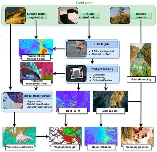
Figure 1.
Overview of the workflow proposed to monitor fine-scale changes at alpine ecosystem boundaries. The workflow is based on UAV surveys, collecting RGB (2 cm resolution), multispectral, thermal and LiDAR data. These datasets are then used to create ancillary datasets (vegetation classification, vegetation height, solar radiation and seedling position), and all results are then linked to an existing field transect, here the monitoring of Fuscospora cliffortioides recruitment.
2.2. Field Preparation for Ground Control Points and Vegetation Ground-Truth Survey
The georeferencing of UAV imagery was dependent on the use of two differential GPS devices (Emlid, Reach RS+, Single-band real-time kinematic GNSS receiver). These devices were employed to map GCPs, which were either 0.5 m2 chessboard-patterned plastic panels or areas marked with high-visibility spray paint. These GCPs were placed within the planned UAV flight paths. They served as reference points for the photogrammetric orthorectification process ensuring accurate spatial alignment of the collected RGB and multispectral UAV imagery. In addition, the differential GPS devices were deployed to record the locations of plant or vegetation patches within the subalpine zone to serve as a ground-truth dataset. At each site, more than 600 point-based plant identifications were conducted to validate vegetation classification outputs.
Optical RGB images were captured using the built-in UAV camera (DJI Phantom 4; SZ DJI Technology Co., Ltd., Shenzhen, China). In addition, the UAV was outfitted with a Parrot Sequoia+ multispectral and sunlight sensor (Parrot SA, Paris, France). This configuration included an extended antenna with the light sensor and the fixed-position, bottom-mounted multispectral sensor acquiring data in seven spectral bands (550–790 nm). Flight plans were devised using Universal Ground Control Station Version 3.1.817 (UgCS; SPH Engineering, Riga, Latvia), along with the compatible Android App “UgCS for DJI” (SPH Engineering, Riga, Latvia). An 8 m resolution DEM for New Zealand (Geographx, Wellington, New Zealand [49]) served as a guide to navigate the UAV at a height of 50 m above ground to avoid canopy obstructions. The weight of the payload restricted the UAV’s flight time to a maximum of 12 min, allowing an area coverage of approximately 200 m × 200 m (4 ha) at a flight speed of 5 m/s.
We performed pre- and post-flight calibrations of the multispectral sensor using the manufacturer-recommended “One-Point Calibration plus Sunshine Sensor” method using the Parrot calibration target plate [50]. Given that the multispectral camera functions independently of the RGB setup, it was programmed to record images onto a “class 10” microSD card at intervals of 4 s. This timing was chosen to align with the UAV’s speed and the overlap requirements of the photogrammetry software. For the purpose of automating the extraction of latitude and longitude data from the image metadata, we employed the “ExifTool” Version 11.5 [51]. The coordinates obtained from the multispectral images were stored in a comma-separated values (csv) file to facilitate further photogrammetric processing.
2.3. Photogrammetry Post-Processing
The photogrammetry software Pix4D version 4.9 (Pix4D, Lausanne, Switzerland) was used to stitch together and georeference the UAV imagery. Processing was performed at 80% along-track overlap, matching the drone pathway traversing alongside the gradient and based on GCPs spanning the entire site. The GCP locations, sourced from the field survey data, were converted from the WGS 1984 geographic projection format to the local New Zealand Transverse Mercator (NZTM 2000) projection. After a preliminary review of the mapped area using the coordinates from the individual images, the footage was processed to align the projection information with the imported georeferenced GCPs. This step was then followed by a re-run and finalisation of the photogrammetry process. The multispectral imagery required an additional step to integrate the extracted coordinates and the reflectance panel values.
In the initial stage of the accuracy assessment during post-processing, the results were imported into ArcGIS Pro v.2.2.3 (ESRI, 2020). This allowed for a visual interpretation of the overlays by employing transparency and swipe tools within the software. These tools facilitated the comparison between RGB and multispectral acquisitions (Figure 2).
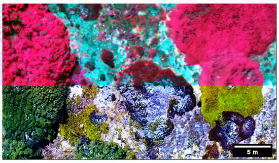
Figure 2.
Comparative display of RGB and multispectral imagery for Mt Faust, New Zealand. This image presents a side-by-side comparison of 5 cm resolution multispectral imagery (displayed in false colour; top section) and 2 cm resolution RGB imagery (bottom section). The purpose is to assess the precision of initial outputs by identifying vegetation boundaries at the study site.
The effectiveness of the orthorectification and alignment of the two image datasets (RGB and multispectral) was assessed by using the GCP labels and identifying unique features within the sites, such as rocks and flowering plants. This involved pinpointing the centre of these features in both spectral layers (see Figure 3). The distances between these corresponding points were then calculated and used as a general indicator of the accuracy in aligning both datasets.
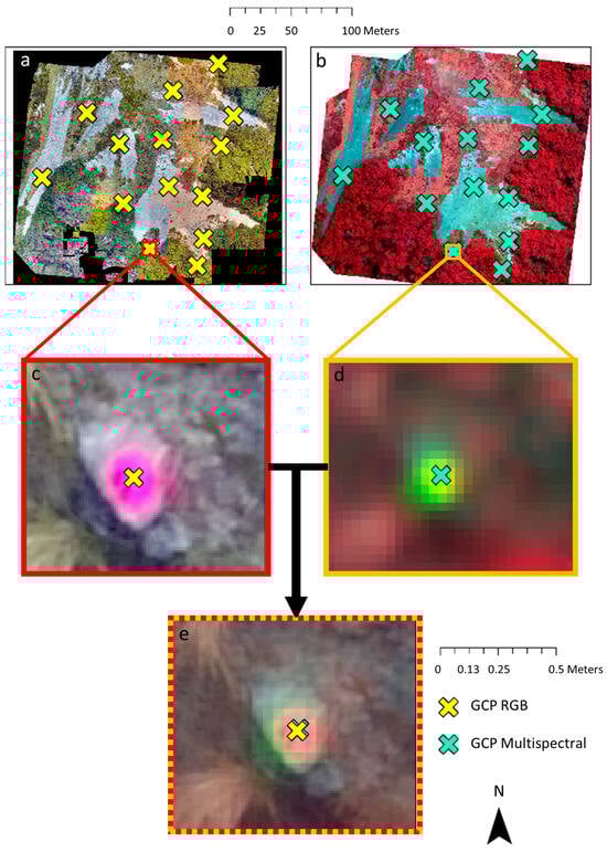
Figure 3.
Accuracy assessment (in terms of Root Mean Square Error, RMSE) of RGB vs. multispectral imagery for the Craigieburn site, New Zealand, by manually selecting GCP centres in ArcGIS Pro. Images (a,c) show the RGB imagery, while (b,d) depict the multispectral imagery with marked GCPs. Image (e) presents an overlay of both spectral layers, enabling the measurement of spatial displacement. The mean offset across all 14 GCP’s between RGB and multispectral imagery was 5.29 ± 2.34 cm.
2.4. Object-Oriented Image Classification Using eCognition Software
For the classification of land cover types from the generated imagery, we employed eCognition Developer 9.0 software (Trimble Geospatial Imaging, Munich, Germany). This process involved an object-based classification approach, which was trained using ground-truth data from the field survey of vegetation. Leveraging all seven spectral bands, we first executed a segmentation process, followed by the implementation of a classification algorithm.
The segmentation was carried out using the “multiresolution segmentation” technique, which was optimized to reduce the average heterogeneity of image objects based on their spectral values (treated with equal weights) [52]. This resulted in an image segmented into objects with spectral homogeneity. The parameters for object “scale”, “shape” and “compactness” were adjusted for each site to accommodate the varying degrees of vegetation heterogeneity. At Mt Faust, due to increased diversity in subalpine species compositions, the size of the generated objects was reduced and decreased, with emphasis placed on the compactness criterion. For this location, we decreased the size of the generated objects, and lowered the weight of the compactness criterion (scale: 100, shape: 0.1, compactness: 0.9), in contrast to the settings used at the Craigieburn site (scale: 250, shape: 0.1, compactness: 0.7). For the Craigieburn site, to reduce hardware processing demands, large areas of bare ground and scree were excluded before classification. This exclusion was based on identifying non-vegetated ground using the multispectral-derived Normalized Difference Vegetation Index (NDVI). To ensure the integrity of the mean spectral response calculations within segmented objects, a rigorous NDVI threshold of 0 was implemented to delineate subalpine vegetation from scree, thereby establishing a definitive boundary at vegetation edges. This approach precludes the potential distortion of spectral mean values by non-vegetative signals, leveraging positive NDVI values as indicators of active photosynthetic activity.
Each object created in the process contained average values of spectral bands along with computed NDVI values. For the consecutive analysis, this implies a hard gap at vegetation boundaries. This was to ensure that, during the segmentation and mean spectral response calculations, the values are not distorted by any plant alive signals. These mean spectral values provided the input for a supervised classification algorithm. The output of this algorithm, in conjunction with the results from the field survey, facilitated the identification of six distinct ground cover classes: bare ground, unvegetated ground (scree), tussock grasses (Chionochloa spp.), mountain beech (Fuscospora cliffortioides) and three types of alpine shrubs (Dracophyllum uniflorum, Leucopogon colensoi, Podocarpus nivalis).
For the training of the algorithm, a nearest neighbour (NN) classifier was employed, which was trained using a selection of field-validated vegetation samples. This approach capitalizes on the distinct spectral reflectance signatures among the identified vegetation types for effective class differentiation. The concern regarding the use of spectral bands that closely resemble each other in their spectral profiles lies in their potential to obscure feature distinctions rather than enhance them. By employing the “Feature Space Optimization” tool, we systematically selected the spectral bands, ensuring that those chosen offered the most significant discriminatory power. Specifically, this facilitated the identification and inclusion of an optimal set of features based on their ability to provide clear separation among vegetation classes. This optimized feature set comprised nine elements: seven spectral bands, plus the NDVI and brightness indices. The optimization process did not merely focus on the proximity of spectral band ranges, but rather on the efficiency of these bands and additional features in maximizing class separability.
To assess the accuracy of the classification, we used an error confusion matrix created in ArcGIS Pro. In brief, 500 points were randomly distributed within the classified area, with each point being assigned the classification value of the underlying area. These values were then manually cross-referenced with the ground-truth data obtained from the field survey. The Kappa statistic was applied to evaluate the overall classification performance.
2.5. Collection of Thermal and LiDAR Data
For the Craigieburn study site, both thermal and LiDAR data were acquired. The thermal imagery was captured using an Altus ORC2 UAV (Altus Intelligence, Hamilton, New Zealand). To analyse diurnal thermal profiles, two flights were conducted in the late austral autumn of the Southern Hemisphere, one in the morning and one in the early afternoon of 20 May 2019. We used a FLIR Duo Pro R thermal sensor, featuring a resolution of 640 × 512 pixels, spectral bands ranging from 7.5 to 13.5 µm, a thermal frame rate of 9 Hz and a 32° field of view (FLIR Systems, Wilsonville, OR, USA).
The LiDAR data collection was performed using the same UAV but on a different flight. This resulted in a comprehensive point cloud dataset for the entire Craigieburn site, with inter-point distances varying from 0.1 m to 0.5 m. The software ArcGIS Pro has been used to calculate a high-resolution digital terrain model (DTM) and digital surface model (DSM) from the point cloud. For the DSM, the 99th percentile of points was selected, while the lowest points were chosen for the DTM. The maximum pulse difference between these two layers was then calculated to develop a vegetation height model, as seen in Figure 4.
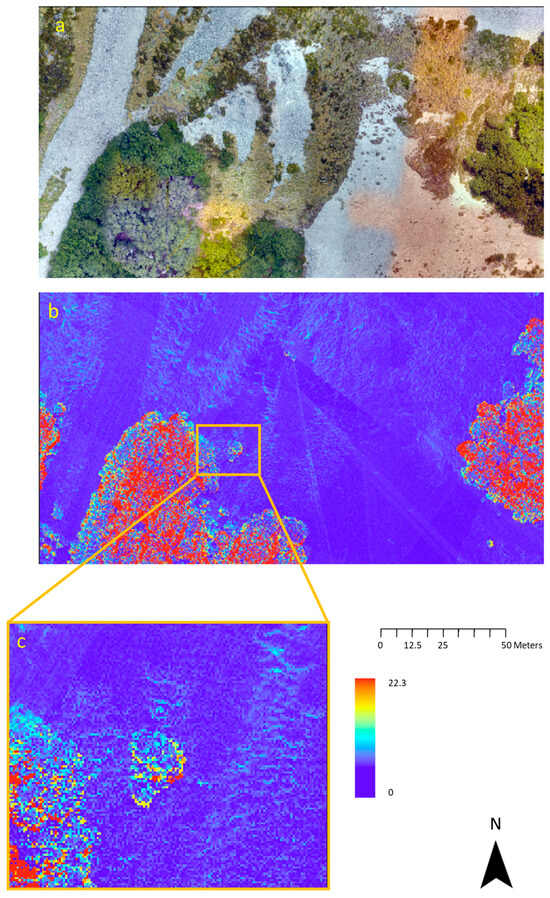
Figure 4.
An RGB image and a point cloud generated from LiDAR data for the Craigieburn site, New Zealand. The image shows (a) an RGB image (2 cm resolution), (b) a vegetation height model (20 cm resolution), and (c) a highlighted vegetation height model for a selected area within the site. The vegetation height data for both topographic features and vegetation are obtained by computing the difference between the DTM and the DSM.
The amount of solar radiation received on particular days at the Craigieburn site can be determined using ArcGIS Pro and the site’s DSM. To calculate the incident radiation, we selected days representative of late autumn and summer in the Southern Hemisphere (20 May and 12 February, respectively). The selected dates align with the periods when ground studies on photoinhibition were conducted at this location [53].
2.6. Spatial Referencing of the Monitored Seedlings
The initial establishment of monitoring transects for treeline seedlings occurred in the austral summer of 1990–1991 [48], with three subsequent re-measurements occurring thereafter. These transects, set parallel to the treeline edge along a predetermined compass bearing, provide detailed data on each seedling’s location, height, diameter and tree tag number. Every seedling within a 20 m distance beyond the treeline edge was included in the transect. The recorded locations were based on measurements taken both “along” and “from” the transect line. Within this study, these transects were re-sampled in 2018–2019. To accurately map seedling positions in the field, the poles marking the transects were georeferenced with centimetre-level precision (Figure 5) using the same differential GPS system employed for the vegetation survey. With the coordinates of the start and end points of the transect, as well as the bearing of the transect line, we were able to spatially calculate the relative location of the seedlings (“along” and “from” measurements) in a GIS, and convert them to the New Zealand Transverse Mercator coordinate system. In ArcGIS Pro, an “offset” function was used to accurately place each seedling in the GIS, based on its “from transect” distance, at a 90° angle to the main transect bearing (Figure 5).
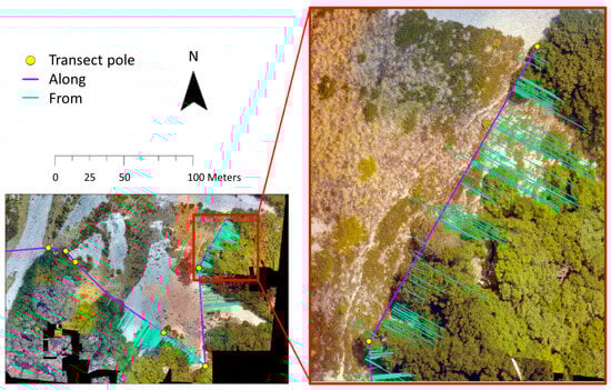
Figure 5.
A 2D representation of seedling transects in the Southern Alps, New Zealand (−43.064°S, 171.425°E, Craigieburn), originally established by P. Wardle in 1991. The positions of seedlings along (X-axis, purple lines) and perpendicular to (Y-axis, teal lines) the transect are derived from the GPS coordinates of marked transect poles (indicated by yellow points).
2.7. Statistical Analysis of Remotely Sensed Temperature Profile
Differences in the maximum daily temperature range (noon temperature minus morning temperature) among ground cover types were analysed using a one-way analysis of variance, carried out in the R software environment (R version 4.1.0, R Core Team). Model diagnostic plots indicated variance heterogeneity, which was accounted for by incorporating a variance function, allowing stratified variance modelling according to the ground cover types (R package nlme, [54]). A post hoc comparison based on Tukey contrasts was performed, and the resulting p-values were multiplicity-adjusted using the false discovery rate method (R package emmeans, [55]). Sample values for the maximum temperature range were derived from a set of 100 manually selected vegetation and scree samples for each class, chosen based on vegetation classification to represent a diverse range of aspects and radiation conditions within the Craigieburn subalpine environment. For each segmented sample, we calculated the maximum daily temperature difference to investigate the temperature range within the subalpine belt.
3. Results
3.1. Object-Based Vegetation Classification
The supervised object-based classification of vegetation, combining both RGB and multispectral channels at the Craigieburn and Mt Faust sites, resulted in high-quality maps depicting six predominant ground cover types found in the alpine treeline ecotone (Figure 6). The integration of GCPs with image metadata facilitated the orthorectification of all RGB and multispectral UAV imagery with centimetre-level precision, enabling accurate measurements of spatial displacement (Craigieburn: 6.14 ± 4.03 cm; Mt Faust: 5.11 ± 2.88 cm). This process achieved a highly accurate depiction of the treeline edge and detailed mapping of vegetation composition in the subalpine zone, as evidenced by the cross-tabulation analysis (Table 1). Notably, the extensive non-vegetated scree slopes at Craigieburn were distinctly separated from areas devoid of healthy vegetation based on the NDVI (>0.1, 98% accuracy). The assessment of these results through a confusion matrix indicated high classification accuracy for both Craigieburn (Kappa = 89.7%) and Mt Faust (Kappa = 71.0%).
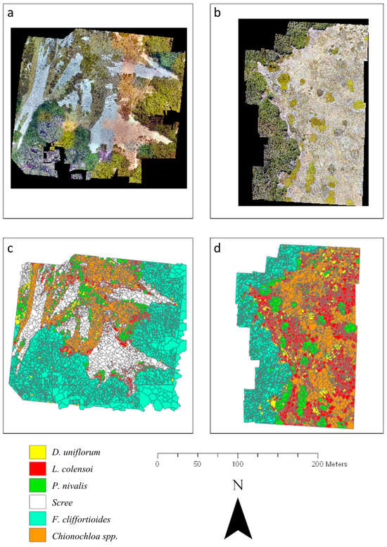
Figure 6.
Results of the vegetation classification for both subalpine treeline ecotones. The figure presents RGB images of (a) Craigieburn and (b) Mt Faust (2 cm resolution), as well as vegetation classification via seven spectral reflectance bands of (c) Craigieburn and (d) Mt Faust (5 cm resolution). Bare ground, unvegetated ground (scree), mountain beech (Fuscospora cliffortioides) and tussock grasses (Chionochloa spp.), and three types of alpine shrubs (Dracophyllum uniflorum, Leucopogon colensoi, Podocarpus nivalis) are clearly distinguished. At Mt Faust, scree areas were lacking.

Table 1.
Accuracy assessment matrix (‘confusion matrix’) for vegetation classification at the Craigieburn and Mt Faust study sites, New Zealand. The Kappa single-value metric evaluates the agreement between classified and actual true values, taking into account both user’s accuracy (U) and producer’s accuracy (P). At Mt Faust, scree areas were lacking. FUSCLI = Fuscospora cliffortioides, LEUCOL = Leucopogon colensoi, DRAUNI = Dracophyllum uniflorum, PODNIV = Podocarpus nivalis, TUSSOCK = Chionochloa spp.
At the Craigieburn site, the most accurate classifications were observed for beech trees and tussock grasses, with less than 10% misclassification. However, the data for L. colensoi and Chionochloa spp. were often confused with each other. The woody species L. colensoi and P. nivalis exhibited the highest levels of classification uncertainty, with 33% and 24% misclassification (in terms of producer’s accuracy), respectively.
At Mt Faust, the highest accuracies were observed for beech trees, with less than 5.5% misclassification. In contrast, Dracophyllum uniflorum and tussock grasses showed higher levels of uncertainty, with misclassification rates of 21% and 33%, respectively. Notably, the classification process demonstrated high accuracy (up to 90%) for larger vegetation associations that encompass multiple spatially-connected objects, such as Podocarpus nivalis and Chionochloa spp. The green and blue spectral bands (from the RGB imagery) and the NDVI calculations (based on multispectral data) proved especially effective in differentiating vegetation classes.
The vegetation classification was used to extract vegetation height from the LiDAR-based vegetation height model. The output was filtered with categorical threshold filters, producing a comprehensive overview of plant height estimates for ~6000 ground cover objects (Table 2).
Table 2.
LiDAR-based mean vegetation height and standard deviation (SD) estimates for the six vegetation classes at the Craigieburn site, New Zealand.
3.2. Radiation and Thermal Mapping
The solar radiation maps generated for this study effectively demonstrated the influence of the sun’s incident angle and intensity on light regimes, with local topography and particularly the orientation of the mountain slopes playing a significant role in modulating exposure. These maps were generated using the Surface Radiation Budget tool within ArcGIS, based on the LiDAR generated DSM (20 cm resolution) of the top vegetation layer at the Craigieburn site. The tool calculates the total solar radiation budget (Wh/m2), factoring in the geographic and temporal specifics to accurately model solar exposure. For this study, solar radiation regimes for the austral summer (12 February) and late autumn (20 May) were analysed to coincide with a field study on photoinhibition [56]. Solar radiation regimes for austral summer and late autumn highlight the strong effect of transpiration cooling in areas with continuous plant cover compared with scree slopes and bare patches within vegetated areas that heat up quickly (Figure 7).
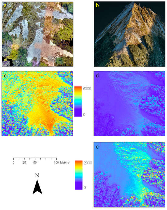
Figure 7.
Calculated solar radiation budget (Wh/m2) for the Craigieburn site, New Zealand (−43.064°S, 171.425°E), based on a DSM (20 cm resolution) generated from LiDAR data (20 May 2019). (a) RGB visualisation (2 cm resolution) and (b) LiDAR generated point cloud visualisation of the site. (c) Predicted solar radiation in Wh/m2 for an entire summer and (d) late autumn day using an (e) adjusted colour scale.
Solar radiation maps based on the DSM (20 cm resolution) revealed clear advantages over standard source material used for flight planning (8 m resolution, Geographx; LINZ, Wellington, New Zealand, 2016). The high-resolution topography layer visualises the effects of slope, aspect and small-scale landscape features (e.g., boulders and trees) in controlling the light regime at the Craigieburn site (Figure 8).
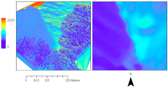
Figure 8.
Effect of DEM resolution in predicting solar radiation regimes. Solar radiation map based on the LiDAR DSM (left, 20 cm resolution) compared with the standard DTM (right, 8 m resolution; LINZ, 2016) source material for Craigieburn site in late austral autumn (20 May 2019).
The thermal imagery captured at the Craigieburn site offered detailed insights into diurnal temperature variations within the alpine treeline ecotone during the late autumn of the Southern Hemisphere (Figure 9). The thermal imagery presented is a raster image processed by Fox and Associates New Zealand, specializing in UAV Aerial Surveying and Mapping. The processing included corrections for geometric distortions to produce accurate, absolute temperature values across the landscape. We reprojected the raster data and displayed it on the LiDAR-generated DSM. These results highlight the influence of various factors, such as time of day, topography, vegetation, and different land cover types (including vegetated and non-vegetated areas) on the thermal environment. A comparative analysis of temperature ranges across different ground cover types (Figure 10) identified considerable differences between non-vegetated (scree) areas and vegetated regions. Apart from areas dominated by Leucopogon colensoi, all ground cover types strongly moderated temperature fluctuations along the eastern slope. This buffering resulted in maximum temperature variations of less than 13 °C (median of the object-specific maxima). In contrast, the scree areas experienced rapid heating, leading to substantially larger temperature variations of around 20 °C during a typical late autumn day. Leucopogon colensoi patches showed little buffering capacity, resulting in a maximum temperature range of 17.7 °C, which differed significantly from the remaining vegetation types, and also from the scree areas.
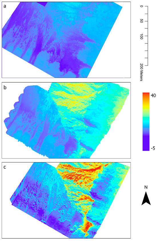
Figure 9.
Results of the UAV thermal surveys at Craigieburn site, New Zealand (late austral autumn, 20 May 2019). Temperature recordings (°C) in the morning (a), at noon (b) and the differences between both surveys (c).
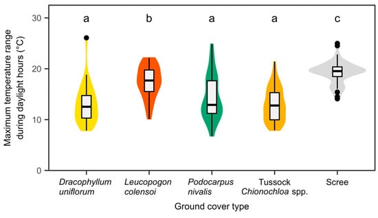
Figure 10.
Box-and-violin plots of the maximum surface temperature range during daylight hours (late autumn) by ground cover type. Maximum differences in surface temperature were derived from UAV-based thermal imaging surveys in the morning and at noon on east-facing slopes of Craigieburn site, New Zealand. Different lower-case letters indicate statistically significant differences at α = 0.05 (post hoc test based on Tukey contrasts).
3.3. Seedling Transect Visualisation
The topography, solar and thermal layers were consecutively combined with the seedling monitoring data. This approach resulted in a detailed overview of the abiotic dynamics on site, providing an “environmental sandbox” to investigate three decades (1991–2021) of seedling regeneration patterns in the subalpine zone (Figure 11). These three decades of data about seedling presence and absence, growth performance and new recruitment can be readily queried within geospatial software, enabling an in-depth study of environmental variables controlling seedling recruitment in the subalpine ecotone [53].
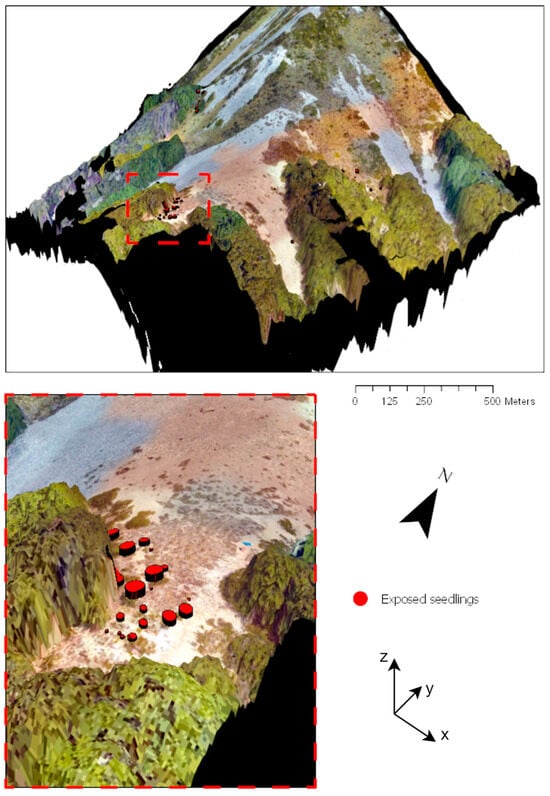
Figure 11.
A 3D-visualisation of the Craigieburn site, New Zealand, with Fuscospora cliffortioides seedling position and height at the treeline. The illustration used UAV-based RGB imagery (2 cm resolution) over the DTM (subalpine zone) and the DSM. Seedling positions were aligned along a long-term vegetation monitoring transect. The symbol size is proportional to seedling height recordings in the summer of 2019.
The UAV-based datasets, with their finer resolution compared to the standard 8 m satellite DTM for this region, offered clear benefits. This was particularly evident in the detailed analysis of topography, solar conditions and seedling monitoring data (Figure 12). The 20 cm LiDAR dataset facilitated an in-depth examination of how individual trees and the nearby treeline affect the radiation environment at this site.
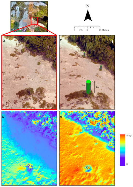
Figure 12.
High-quality LiDAR DSM layer (20 cm resolution) used for calculation of shading potential of individual trees at the treeline (a,b) of the Craigieburn site, New Zealand. The procedure enabled (c) 3D visualisations of exposed Fuscospora cliffortioides trees (green cylinder), measured as part of a treeline monitoring programme. Solar radiation projections (Wh/m2) illustrate the shading potential of individual trees in (d) late austral autumn and (e) summer.
By combining the top vegetation LiDAR DSM with a resolution of 20 cm and thermal data (comparing morning and noon temperatures), we were able to accurately map thermal patterns in the alpine treeline ecotone. This approach also facilitated the analysis of correlations with solar radiation budgets (Wh/m2) during the late autumn in the Southern Hemisphere (Figure 13).
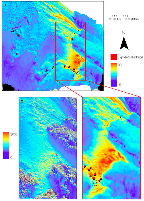
Figure 13.
A 3D-visualisation of the Craigieburn site, New Zealand, with tree seedling positions and heights (indicated by symbol size). (a,c) Thermal differences (late austral autumn, 20 May 2019, morning vs. noon) above canopy draped over the LiDAR DSM (20 cm resolution). Seedling positions from a treeline census dataset are located along the transect, and their heights (summer 2019) are displayed and compared with (b) calculated solar radiation (Wh/m2) for the same late austral autumn day.
4. Discussion
Using a novel approach of UAV-mounted RGB and multispectral cameras for dual image capture, we effectively developed a comprehensive classification of the alpine treeline ecotone. This was further improved by integrating the imagery with topographical, thermal and solar radiation maps and connecting these with thirty years of seedling monitoring data. Our approach provides a data-rich resource, permitting an in-depth analysis of the role of abiotic limitations in sharpening the ecotone transition at the treeline.
Our study significantly advances the field with its centimeter-scale resolution datasets, offering a more detailed exploration of the alpine treeline ecotone than previously possible. Contrasting with prior research [28] that deployed UAV, LiDAR and satellite imagery at lower resolutions for studying tree mortality, our methodology integrates high-resolution UAV imagery with extensive ecological data to delineate ecotone transitions precisely. This approach surpasses the broader applications and ecosystem focuses typical of earlier studies [30,36,57] by creating a direct link between advanced UAV technology and long-term monitoring data to identify specific abiotic factors driving treeline dynamics. Our innovative use of methodological precision and comprehensive environmental variable integration allows for a nuanced examination of treeline transitions, setting our work apart in the ecological field and significantly enhancing our understanding of alpine treeline ecotone dynamics and the abiotic limitations that shape them.
In particular, the use of multispectral-derived NDVI data for defining vegetation boundaries demonstrated increased accuracy (Table 1). Our research underscores the valuable combination of UAV technology, high-resolution data and vegetation indices in effectively mapping vegetation cover [13,16]. Using the proposed approach, we achieved a clear distinction between vegetation types, with only minor inconsistencies for more densely grouped plant associations such as Dracophyllum spp. and Podocarpus nivalis, with 60–90% or 60–80% overall classification accuracy, respectively. These inconsistencies were due to extensive spectral overlap in the bands used to discriminate species (>30%, NDVI, green (RGB)) and the minimum object size used in the classification algorithm. The high accuracy is comparable to other UAV vegetation segmentation studies [37,58,59,60] and superior to the overall accuracy reported from a recent UAV survey across a Norwegian treeline ecotone, with similar resolution and classification features but differing classification algorithms [61]. Our findings suggest that the proposed technique provides a powerful approach to improving aerial mapping at the vegetation community, habitat and possibly species scales. Adopting this technique into practice can greatly facilitate conservation efforts, natural resource management and landscape planning.
Previous studies at lower elevations showed that the highest classification accuracy was achieved with data recorded at peak growing season [62,63,64]. The timing of the data collection during the short alpine growing season may therefore have a strong influence on classification accuracy. From this point of view, the timing of our flights in the late growing season was suboptimal but yielded very high accuracy, nonetheless. This is in line with recent findings from a vast treeline transect in Scandinavia demonstrating that classification performance is neither significantly affected by the timing of the aerial survey within the growing season, nor by geographical variations within such heterogeneous habitats [61].
Airborne LiDAR sensors provide state-of-the-art, high-resolution topography layers [19,22,23] and represent the source for ancillary datasets, e.g., information on solar radiation and vegetation height. In this study, the sensor resolution was a limiting factor for consistently accurate plant height estimates. However, this issue can be mitigated by employing higher quality sensors and increasing sampling rates, which would allow for more thorough penetration through vegetation cover [13]. The final LiDAR digital surface models gave estimates of microhabitat height for ~6000 classified vegetation objects within the Craigieburn site. These estimates can be used to study mechanical insulation effects (e.g., facilitative feedback [11]), as recently demonstrated within these vegetation microhabitats [53].
We were able to calculate inter-annual variation in the solar radiation budget at the treeline based on the LiDAR-derived DSM. The high resolution of this surface layer revealed that seedlings near the existing treeline on east-facing slopes experience almost constant shade around the winter solstice (Figure 12). This insight is particularly important for treeline sites where growth is thought to be hindered by cold-induced photoinhibition, a concept supported by various studies [56,65,66,67,68]. Recent findings underscored the complexity of the diurnal radiation budget on sloping terrain in alpine environments [69]. Our findings suggest that, when an alpine treeline ecotone is limited by both frost and high solar radiation (photoinhibition), yet seedlings manage to establish in areas of prolonged shade during late autumn, then this can inform the optimal timing for studies focusing on these recruitment bottlenecks. From a practical perspective, this information can also be helpful in certain areas for the restoration of treeline woodlands or high-elevation protection forests, which have undergone severe shrinkage and degradation in recent decades [70].
The east-facing scree slopes at the Craigieburn site heated up rapidly during the day, with temperature differences reaching up to 25 °C between morning and noon flights (Figure 10). Highly detailed topography data from LiDAR measurements was instrumental in accurately mapping the thermal profiles derived from infrared imaging [71]. The fine-scale 3D-thermal profile of the subalpine belt gives detailed insight into the spatial heterogeneity of surface temperatures and is, thus, a vital tool for determining the effects of topography and vegetation on the microclimatic conditions on site. In a wider context, our approach facilitates research that critically relies on micrometeorological and plant physiological data (multispectral indices), such as studies on thermal acclimation and adaptation associated with thermal niche modelling.
In line with our findings, [72] demonstrated that LiDAR-produced vegetation height models can further refine the vegetation segmentation process. The identification of taller, exposed features of plant communities helps our understanding of the role of humidity, solar radiation and wind speed in controlling the thermal environment and temperature relations of plants [73,74]. Our UAV thermal imaging flyovers allowed determination of the temperature ranges during daylight hours (morning vs. noon, late austral autumn) as a function of ground cover type on the predominantly east-facing slope at the Craigieburn site (Figure 9 and Figure 10). It is well-documented that the (sub)alpine vegetation creates a temperature buffering effect, largely determined by growth habit and transpiration cooling [3]. Based on this buffering effect, we assumed smaller temperature variations on vegetated surfaces compared with the scree slopes. This assumption was confirmed by the infrared-based temperature measurements, which clearly illustrated the vegetation-driven thermal buffering phenomenon, except for L. colensoi. For this shrub species, the spreading, somewhat loosely arranged branches provide a sparse growth habit, probably causing closer coupling to the prevailing meteorological conditions compared with the more compact growth of co-occurring species. Plant architectural effects on canopy temperature have been documented before [12]; however, temperature variation may also be linked to differences in plant water use [75]. As expected, temperature fluctuated more widely on scree slopes and bare patches nestled within vegetated areas, highlighting the temperature variability on the microhabitat scale and the importance of the resulting mosaic of thermal niches for (sub)alpine biodiversity [12,76]. The magnitude of the temperature buffering effect commonly increases towards the centre of the plant body, but infrared sensors cannot penetrate deeply into the complex structure of dwarf shrubs or the clumped growth form of tussocks. For this reason, surface temperatures may not reflect the full buffering capacity [3].
Our approach of retrospectively georeferencing seedling transect surveys made it possible to link occurrence data with relevant ecological factors. It also revealed great potential for elucidating the role of microhabitat characteristics for seedling establishment. Although UAV flyovers from a single day cannot provide comprehensive information of environmental processes, the data we gleaned from this campaign provides extraordinary insight into the factors shaping spatial patterns of species occurrence. At the same time, this information supports spatially explicit modelling [56]. Furthermore, multiple UAV flights throughout the year can help capture temporal variability, allowing for detailed studies of seedling performance (recruitment, growth, mortality) in relation to microhabitat characteristics (topography, thermal, solar radiation) and ground cover type.
The combination of high-resolution spectral and topographic data with long-term vegetation sampling reveals new potential in existing vegetation monitoring plots. This added dimension to established monitoring frameworks can be a key driver in unravelling the complex dynamics at treeline ecotones [77]. A number of studies have highlighted the considerable potential of UAV research to produce high-resolution spatial datasets and bridge the gap between satellite and field data [27]. However, they remain a spatially explicit snapshot of the environmental conditions on site neglecting the temporal dynamics. This study introduced a novel workflow to address this limitation by pairing UAV imaging with long-term vegetation mapping campaigns to better exploit the potential of both data sources for studying vegetation dynamics. The results can be used to monitor seedling performance in a spatially explicit context and further investigate current recruitment bottlenecks, which are of particular interest in studies on slow ecotone dynamics and transplant experiments [11,53]. In addition, this workflow may provide enhanced support for conservation actions and decision-making, especially when dealing with vast monitoring areas and/or poorly regenerating species [78]. The methodology is currently mainly limited by the spatial resolution of the sensors, and the “weakest link” is the poorest resolution dataset used for the interpretation [8]. In studies with a strong emphasis on physiological processes, the spectral resolution of the multispectral sensor may also become limiting, which can be overcome by switching to a hyperspectral system [79]. The rapid advances in sensor technology and ease of use of UAV workflows are already paving the way for novel high-resolution learning segmentation processes [80]. UAV surveys are rapidly becoming standard practice, allowing for further exploitation of the “environmental sandbox” created, leveraging spectral signatures of phenological stages for the segmentation process [81] or monitoring treatment effects on vegetation distribution (e.g., weed spraying, [82]). We advocate monitoring complex ecosystem interactions with repeated UAV surveys to achieve a more comprehensive overview of the multi-dimensional plant-environment interactions at scale.
5. Conclusions
Ecotones in general, and their boundaries in particular, are sensitive indicators for climate change because many of the species present live very close to their tolerance limits [83]. However, tracking (subtle) shifts in vegetation dynamics, such as seedling regeneration in response to environmental change, requires periodic observations, which are notoriously difficult to obtain in case of ground-based measurements in such inaccessible, remote areas. The urgent need to closely monitor, understand and predict ecotone changes calls for a cost-effective, readily applicable remote sensing framework, like the proposed multi-pronged approach linking UAV-based optical multispectral and thermal data as well as LiDAR data with permanent sampling plots. Although we tested this novel approach in a treeline ecotone setting, it is readily applicable to other habitats and more general research questions. Our high delineation and identification accuracy allows improved vegetation and habitat mapping for conservation, ecosystem management and ecological risk assessment. The high accuracy, together with the infrared data, facilitates research into the variation in thermal niches under climate change. Further exploitation of the multispectral data can shed light on physiological processes and their responses to shifting environmental conditions. Leveraging the complementary strengths of these remote sensing tools allows deeper insights into ecosystem dynamics and more efficient responses to pressing ecological challenges.
Author Contributions
F.D. developed the workflows, acquired the data and had the lead role in writing the manuscript. M.K.-F.B. supervised the research and co-wrote and shaped the manuscript. J.E.S.F. provided critical feedback and helped shape the manuscript. All authors have read and agreed to the published version of the manuscript.
Funding
This research received no external funding.
Data Availability Statement
The data presented in this study are available on request from the corresponding author.
Acknowledgments
Support for this research was provided by Auckland University of Technology (AUT, Auckland). We would like to thank the Department of Conservation (DOC) for access permissions, as well as Lincoln University and Boyle Outdoor Education Centre (Canterbury, New Zealand) for providing accommodation and field equipment. We would like to thank Bradley S. Case for kindly providing the funding for the thermal and LiDAR UAV flights. We are grateful to Katrin Berkenbusch for her valuable comments on the final version of the manuscript.
Conflicts of Interest
The authors declare that they have no competing financial interests or personal relationships that could have appeared to influence the work reported in this paper.
References
- Gosz, J.R. Ecotone Hierarchies. Ecol. Appl. 1993, 3, 369–376. [Google Scholar] [CrossRef]
- Wasson, K.; Woolfolk, A.; Fresquez, C. Ecotones as Indicators of Changing Environmental Conditions: Rapid Migration of Salt Marsh–Upland Boundaries. Estuaries Coasts 2013, 36, 654–664. [Google Scholar] [CrossRef]
- Körner, C. Alpine Treelines: Functional Ecology of the Global High Elevation Tree Limits; Springer: Basel, Switzerland, 2012. [Google Scholar]
- Körner, C.; Hiltbrunner, E. The 90 Ways to Describe Plant Temperature. Perspect. Plant Ecol. Evol. Syst. 2018, 30, 16–21. [Google Scholar] [CrossRef]
- Gunderson, L.H.; Allen, C.R.; Holling, C.S. Foundations of Ecological Resilience; Island Press: Washington, DC, USA, 2012; ISBN 978-1-61091-133-7. [Google Scholar]
- Elliott, G.P. Extrinsic Regime Shifts Drive Abrupt Changes in Regeneration Dynamics at Upper Treeline in the Rocky Mountains, USA. Ecology 2012, 93, 1614–1625. [Google Scholar] [CrossRef]
- Holtmeier, F.-K. Mountain Timberlines: Ecology, Patchiness, and Dynamics, 2nd ed.; Advances in Global Change Research; Springer: Dordrecht, The Netherlands, 2009; ISBN 978-1-4020-9704-1. [Google Scholar]
- Weiss, D. Alpine Treeline Ecotones in the Western United States: A Multi-Scale Comparative Analysis of Environmental Factors Influencing Pattern-Process Relations. Ph.D. Thesis, University of North Carolina, Chapel Hill, NC, USA, 2009. [Google Scholar]
- Malanson, G.P.; Resler, L.M.; Bader, M.Y.; Holtmeier, F.-K.; Butler, D.R.; Weiss, D.J.; Daniels, L.D.; Fagre, D.B. Mountain Treelines: A Roadmap for Research Orientation. Arct. Antarct. Alp. Res. 2011, 43, 11. [Google Scholar] [CrossRef]
- Hansson, A.; Shulmeister, J.; Dargusch, P.; Hill, G. A Review of Factors Controlling Southern Hemisphere Treelines and the Implications of Climate Change on Future Treeline Dynamics. Agric. For. Meteorol. 2023, 332, 109375. [Google Scholar] [CrossRef]
- Harsch, M.A.; Bader, M.Y. Treeline Form—A Potential Key to Understanding Treeline Dynamics. Glob. Ecol. Biogeogr. 2011, 20, 582–596. [Google Scholar] [CrossRef]
- Scherrer, D.; Körner, C. Topographically Controlled Thermal-Habitat Differentiation Buffers Alpine Plant Diversity against Climate Warming. J. Biogeogr. 2011, 38, 406–416. [Google Scholar] [CrossRef]
- Weiss, D.J.; Walsh, S.J. Remote Sensing of Mountain Environments. Geogr. Compass 2009, 3, 1–21. [Google Scholar] [CrossRef]
- Lu, B.; He, Y. Species Classification Using Unmanned Aerial Vehicle (UAV)-Acquired High Spatial Resolution Imagery in a Heterogeneous Grassland. ISPRS J. Photogramm. Remote Sens. 2017, 128, 73–85. [Google Scholar] [CrossRef]
- Duro, D.; Coops, N.; Wulder, M.; Han, T. Development of a Large Area Biodiversity Monitoring Driven by Remote Sensing. Prog. Phys. Geogr. 2007, 31, 235–260. [Google Scholar] [CrossRef]
- Chen, J.; Yi, S.; Qin, Y.; Wang, X. Improving Estimates of Fractional Vegetation Cover Based on UAV in Alpine Grassland on the Qinghai–Tibetan Plateau. Int. J. Remote Sens. 2016, 37, 1922–1936. [Google Scholar] [CrossRef]
- Chen, Y.; Lu, D.; Luo, G.; Huang, J. Detection of Vegetation Abundance Change in the Alpine Tree Line Using Multitemporal Landsat Thematic Mapper Imagery. Int. J. Remote Sens. 2015, 36, 4683–4701. [Google Scholar] [CrossRef]
- Ørka, H.O.; Wulder, M.A.; Gobakken, T.; Næsset, E. Subalpine Zone Delineation Using LiDAR and Landsat Imagery. Remote Sens. Environ. 2012, 119, 11–20. [Google Scholar] [CrossRef]
- Šašak, J.; Gallay, M.; Kaňuk, J.; Hofierka, J.; Minár, J. Combined Use of Terrestrial Laser Scanning and UAV Photogrammetry in Mapping Alpine Terrain. Remote Sens. 2019, 11, 2154. [Google Scholar] [CrossRef]
- Morgan, B.; Chipman, J.; Bolger, D.; Dietrich, J. Spatiotemporal Analysis of Vegetation Cover Change in a Large Ephemeral River: Multi-Sensor Fusion of Unmanned Aerial Vehicle (UAV) and Landsat Imagery. Remote Sens. 2020, 13, 51. [Google Scholar] [CrossRef]
- Mathew, J.R.; Singh, C.P.; Solanki, H.; Sedha, D.; Pandya, M.R.; Bhattacharya, B.K. Role of LiDAR Remote Sensing in Identifying Physiognomic Traits of Alpine Treeline: A Global Review. Trop. Ecol. 2023. [Google Scholar] [CrossRef]
- Cawood, A.J.; Bond, C.E.; Howell, J.A.; Butler, R.W.H.; Totake, Y. LiDAR, UAV or Compass-Clinometer? Accuracy, Coverage and the Effects on Structural Models. J. Struct. Geol. 2017, 98, 67–82. [Google Scholar] [CrossRef]
- Gallay, M.; Lloyd, C.D.; McKinley, J.; Barry, L. Assessing Modern Ground Survey Methods and Airborne Laser Scanning for Digital Terrain Modelling: A Case Study from the Lake District, England. Comput. Geosci. 2013, 51, 216–227. [Google Scholar] [CrossRef]
- Villoslada, M.; Bergamo, T.F.; Ward, R.D.; Burnside, N.G.; Joyce, C.B.; Bunce, R.G.H.; Sepp, K. Fine Scale Plant Community Assessment in Coastal Meadows Using UAV Based Multispectral Data. Ecol. Indic. 2020, 111, 105979. [Google Scholar] [CrossRef]
- Candiago, S.; Remondino, F.; De Giglio, M.; Dubbini, M.; Gattelli, M. Evaluating Multispectral Images and Vegetation Indices for Precision Farming Applications from UAV Images. Remote Sens. 2015, 7, 4026–4047. [Google Scholar] [CrossRef]
- Rhodes, C.J.; Henrys, P.; Siriwardena, G.M.; Whittingham, M.J.; Norton, L.R. The Relative Value of Field Survey and Remote Sensing for Biodiversity Assessment. Methods Ecol. Evol. 2015, 6, 772–781. [Google Scholar] [CrossRef]
- Alvarez-Vanhard, E.; Houet, T.; Mony, C.; Lecoq, L.; Corpetti, T. Can UAVs Fill the Gap between in Situ Surveys and Satellites for Habitat Mapping? Remote Sens. Environ. 2020, 243, 111780. [Google Scholar] [CrossRef]
- Campbell, M.J.; Dennison, P.E.; Tune, J.W.; Kannenberg, S.A.; Kerr, K.L.; Codding, B.F.; Anderegg, W.R.L. A Multi-Sensor, Multi-Scale Approach to Mapping Tree Mortality in Woodland Ecosystems. Remote Sens. Environ. 2020, 245, 111853. [Google Scholar] [CrossRef]
- Hernández-Clemente, R.; Hornero, A.; Mottus, M.; Penuelas, J.; González-Dugo, V.; Jiménez, J.C.; Suárez, L.; Alonso, L.; Zarco-Tejada, P.J. Early Diagnosis of Vegetation Health from High-Resolution Hyperspectral and Thermal Imagery: Lessons Learned From Empirical Relationships and Radiative Transfer Modelling. Curr. For. Rep 2019, 5, 169–183. [Google Scholar] [CrossRef]
- Smigaj, M.; Agarwal, A.; Bartholomeus, H.; Decuyper, M.; Elsherif, A.; de Jonge, A.; Kooistra, L. Thermal Infrared Remote Sensing of Stress Responses in Forest Environments: A Review of Developments, Challenges, and Opportunities. Curr. For. Rep. 2023. [Google Scholar] [CrossRef]
- Smigaj, M.; Gaulton, R.; Suárez, J.C.; Barr, S.L. Combined Use of Spectral and Structural Characteristics for Improved Red Band Needle Blight Detection in Pine Plantation Stands. For. Ecol. Manag. 2019, 434, 213–223. [Google Scholar] [CrossRef]
- Dobosz, B.; Gozdowski, D.; Koronczok, J.; Žukovskis, J.; Wójcik-Gront, E. Evaluation of Maize Crop Damage Using UAV-Based RGB and Multispectral Imagery. Agriculture 2023, 13, 1627. [Google Scholar] [CrossRef]
- Fevgas, G.; Lagkas, T.; Argyriou, V.; Sarigiannidis, P. Detection of Biotic or Abiotic Stress in Vineyards Using Thermal and RGB Images Captured via IoT Sensors. IEEE Access 2023, 11, 105902–105915. [Google Scholar] [CrossRef]
- Wei, L.; Yang, H.; Niu, Y.; Zhang, Y.; Xu, L.; Chai, X. Wheat Biomass, Yield, and Straw-Grain Ratio Estimation from Multi-Temporal UAV-Based RGB and Multispectral Images. Biosyst. Eng. 2023, 234, 187–205. [Google Scholar] [CrossRef]
- Berger, K.; Machwitz, M.; Kycko, M.; Kefauver, S.C.; Van Wittenberghe, S.; Gerhards, M.; Verrelst, J.; Atzberger, C.; van der Tol, C.; Damm, A.; et al. Multi-Sensor Spectral Synergies for Crop Stress Detection and Monitoring in the Optical Domain: A Review. Remote Sens. Environ. 2022, 280, 113198. [Google Scholar] [CrossRef]
- Groos, A.; Aeschbacher, R.; Fischer, M.; Kohler, N.; Mayer, C.; Senn-Rist, A. Accuracy of UAV Photogrammetry in Glacial and Periglacial Alpine Terrain: A Comparison with Airborne and Terrestrial Datasets. Front. Remote Sens. 2022, 3, 871994. [Google Scholar] [CrossRef]
- Yan, Y.; Deng, L.; Liu, X.; Zhu, L. Application of UAV-Based Multi-Angle Hyperspectral Remote Sensing in Fine Vegetation Classification. Remote Sens. 2019, 11, 2753. [Google Scholar] [CrossRef]
- Blaschke, T.; Hay, G.J.; Kelly, M.; Lang, S.; Hofmann, P.; Addink, E.; Queiroz Feitosa, R.; van der Meer, F.; van der Werff, H.; van Coillie, F.; et al. Geographic Object-Based Image Analysis—Towards a New Paradigm. ISPRS J. Photogramm. Remote Sens. 2014, 87, 180–191. [Google Scholar] [CrossRef]
- Fabbri, S.; Grottoli, E.; Armaroli, C.; Ciavola, P. Using High-Spatial Resolution UAV-Derived Data to Evaluate Vegetation and Geomorphological Changes on a Dune Field Involved in a Restoration Endeavour. Remote Sens. 2021, 13, 1987. [Google Scholar] [CrossRef]
- Wei, T.; Shangguan, D.; Yi, S.; Ding, Y. Characteristics and Controls of Vegetation and Diversity Changes Monitored with an Unmanned Aerial Vehicle (UAV) in the Foreland of the Urumqi Glacier No. 1, Tianshan, China. Sci. Total Environ. 2021, 771, 145433. [Google Scholar] [CrossRef] [PubMed]
- Wardle, P. New Zealand Forest to Alpine Transitions in Global Context. Arct. Antarct. Alp. Res. 2008, 40, 240–249. [Google Scholar] [CrossRef]
- Leathwick, J.R. Are New Zealand’s Nothofagus Species in Equilibrium with Their Environment? J. Veg. Sci. 1998, 9, 719–732. [Google Scholar] [CrossRef]
- Mcglone, M.; Duncan, R.; Heenan, P. Endemism, Species Selection and the Origin and Distribution of the Vascular Plant Flora of New Zealand. J. Biogeogr. 2002, 28, 199–216. [Google Scholar] [CrossRef]
- Batllori, E.; Camarero, J.J.; Ninot, J.M.; Gutiérrez, E. Seedling Recruitment, Survival and Facilitation in Alpine Pinus Uncinata Tree Line Ecotones. Implications and Potential Responses to Climate Warming. Glob. Ecol. Biogeogr. 2009, 18, 460–472. [Google Scholar] [CrossRef]
- Elliott, G.P. Influences of 20th-Century Warming at the Upper Tree Line Contingent on Local-Scale Interactions: Evidence from a Latitudinal Gradient in the Rocky Mountains, USA. Glob. Ecol. Biogeogr. 2011, 20, 46–57. [Google Scholar] [CrossRef]
- Elliott, G.P.; Kipfmueller, K.F. Multi-Scale Influences of Slope Aspect and Spatial Pattern on Ecotonal Dynamics at Upper Treeline in the Southern Rocky Mountains, U.S.A. Arct. Antarct. Alp. Res. 2010, 42, 45–56. [Google Scholar] [CrossRef]
- Harsch, M.A. Treeline Dynamics: Pattern and Process at Multiple Spatial Scales. Ph.D. Thesis, Lincoln University, Lincoln, New Zealand, 2010. [Google Scholar]
- Harsch, M.A.; Buxton, R.; Duncan, R.P.; Hulme, P.E.; Wardle, P.; Wilmshurst, J. Causes of Tree Line Stability: Stem Growth, Recruitment and Mortality Rates over 15 Years at New Zealand Nothofagus Tree Lines. J. Biogeogr. 2012, 39, 2061–2071. [Google Scholar] [CrossRef]
- LINZ NZ 8m Digital Elevation Model 2016. Available online: https://data.linz.govt.nz/layer/51768-nz-8m-digital-elevation-model-2012/ (accessed on 12 January 2024).
- Poncet, A.M.; Knappenberger, T.; Brodbeck, C.; Fogle, M.; Shaw, J.N.; Ortiz, B.V. Multispectral UAS Data Accuracy for Different Radiometric Calibration Methods. Remote Sens. 2019, 11, 1917. [Google Scholar] [CrossRef]
- Harvey, P. ExifTool, Version 11.5. 2020. Available online: https://exiftool.org/ (accessed on 12 January 2024).
- Trimble eCognition, Version 9.5; Trimble Geospatial: Trimble, CO, USA, 2020.
- Döweler, F. Causes of Recruitment Limitation at Abrupt Alpine Treelines. Ph.D. Thesis, Auckland University of Technology, Auckland, New Zealand, 2021. [Google Scholar]
- Pinheiro, J.; Bates, D. R Core Team Nlme: Linear and Nonlinear Mixed Effects Models; R Package Team: Vienna, Austria, 2023. [Google Scholar]
- Lenth, R.V.; Bolker, B.; Buerkner, P.; Giné-Vázquez, I.; Herve, M.; Jung, M.; Love, J.; Miguez, F.; Riebl, H.; Singmann, H. Emmeans: Estimated Marginal Means, Aka Least-Squares Means; R Core Team: Vienna, Austria, 2024. [Google Scholar]
- Döweler, F.; Case, B.S.; Buckley, H.L.; Bader, M.K.-F. High Light-Induced Photoinhibition Is Not Limiting Seedling Establishment at Abrupt Treeline Ecotones in New Zealand. Tree Physiol. 2021, 41, 2034–2045. [Google Scholar] [CrossRef] [PubMed]
- Nuradili, P.; Zhou, J.; Zhou, X.; Ma, J.; Wang, Z.; Meng, L.; Tang, W.; Meng, Y. UAV Remote-Sensing Image Semantic Segmentation Strategy Based on Thermal Infrared and Multispectral Image Features. IEEE J. Miniaturization Air Space Syst. 2023, 4, 311–319. [Google Scholar] [CrossRef]
- Ahmed, O.S.; Shemrock, A.; Chabot, D.; Dillon, C.; Williams, G.; Wasson, R.; Franklin, S.E. Hierarchical Land Cover and Vegetation Classification Using Multispectral Data Acquired from an Unmanned Aerial Vehicle. Int. J. Remote Sens. 2017, 38, 2037–2052. [Google Scholar] [CrossRef]
- Ishida, T.; Kurihara, J.; Viray, F.A.; Namuco, S.B.; Paringit, E.C.; Perez, G.J.; Takahashi, Y.; Marciano, J.J. A Novel Approach for Vegetation Classification Using UAV-Based Hyperspectral Imaging. Comput. Electron. Agric. 2018, 144, 80–85. [Google Scholar] [CrossRef]
- Marcial-Pablo, M.d.J.; Gonzalez-Sanchez, A.; Jimenez-Jimenez, S.I.; Ontiveros-Capurata, R.E.; Ojeda-Bustamante, W. Estimation of Vegetation Fraction Using RGB and Multispectral Images from UAV. Int. J. Remote Sens. 2019, 40, 420–438. [Google Scholar] [CrossRef]
- Mienna, I.M.; Klanderud, K.; Ørka, H.O.; Bryn, A.; Bollandsås, O.M. Land Cover Classification of Treeline Ecotones along a 1100 Km Latitudinal Transect Using Spectral- and Three-Dimensional Information from UAV-Based Aerial Imagery. Remote Sens. Ecol. Conserv. 2022, 8, 536–550. [Google Scholar] [CrossRef]
- Gränzig, T.; Schuster, C.; Kleinschmit, B.; Förster, M. Evaluating an Intra-Annual Time Series for Grassland Classification—How Many Acquisitions and What Seasonal Origin Are Optimal? IEEE J. Sel. Top. Appl. Earth Obs. Remote Sens. 2014, 7, 3428–3439. [Google Scholar] [CrossRef]
- Feilhauer, H.; Schmidtlein, S. On Variable Relations between Vegetation Patterns and Canopy Reflectance. Ecol. Inform. 2011, 6, 83–92. [Google Scholar] [CrossRef]
- Bradter, U.; O’Connell, J.; Kunin, W.E.; Boffey, C.W.H.; Ellis, R.J.; Benton, T.G. Classifying Grass-Dominated Habitats from Remotely Sensed Data: The Influence of Spectral Resolution, Acquisition Time and the Vegetation Classification System on Accuracy and Thematic Resolution. Sci. Total Environ. 2020, 711, 134584. [Google Scholar] [CrossRef] [PubMed]
- Ball, M.C.; Hodges, V.S.; Laughlin, G.P. Cold-Induced Photoinhibition Limits Regeneration of Snow Gum at Tree-Line. Funct. Ecol. 1991, 5, 663–668. [Google Scholar] [CrossRef]
- Germino, M.J.; Smith, W.K.; Resor, A.C. Conifer Seedling Distribution and Survival in an Alpine-Treeline Ecotone. Plant Ecol. 2002, 162, 157–168. [Google Scholar] [CrossRef]
- Reyes-Díaz, M.; Alberdi, M.; Piper, F.; Bravo, L.; Corcuera, L. Low Temperature Responses of Nothofagus Dombeyi and Nothofagus Nitida, Two Evergreen Species from South Central Chile. Tree Physiol. 2005, 25, 1389–1398. [Google Scholar] [CrossRef]
- Sakai, A.; Paton, D.M.; Wardle, P. Freezing Resistance of Trees of the South Temperate Zone, Especially Subalpine Species of Australasia. Ecology 1981, 62, 563–570. [Google Scholar] [CrossRef]
- Ramtvedt, E.N.; Gobakken, T.; Næsset, E. Fine-Spatial Boreal–Alpine Single-Tree Albedo Measured by UAV: Experiences and Challenges. Remote Sens. 2022, 14, 1482. [Google Scholar] [CrossRef]
- Watts, S.; Jump, A. The Benefits of Mountain Woodland Restoration. Restor. Ecol. 2022, 30, e13701. [Google Scholar] [CrossRef]
- Boesch, R. Thermal Remote Sensing with Uav-Based Workflows. ISPRS—Int. Arch. Photogramm. Remote Sens. Spat. Inf. Sci. 2017, XLII-2/W6, 41–46. [Google Scholar] [CrossRef]
- Weinstein, B.G.; Marconi, S.; Bohlman, S.; Zare, A.; White, E. Individual Tree-Crown Detection in RGB Imagery Using Semi-Supervised Deep Learning Neural Networks. Remote Sens. 2019, 11, 1309. [Google Scholar] [CrossRef]
- Leinonen, I.; Grant, O.M.; Tagliavia, C.P.P.; Chaves, M.M.; Jones, H.G. Estimating Stomatal Conductance with Thermal Imagery. Plant Cell Environ. 2006, 29, 1508–1518. [Google Scholar] [CrossRef] [PubMed]
- Smigaj, M.; Gaulton, R.; Barr, S.; Suarez Minguez, J. Uav-Borne Thermal Imaging for Forest Health Monitoring: Detection of Disease-Induced Canopy Temperature Increase. ISPRS—Int. Arch. Photogramm. Remote Sens. Spat. Inf. Sci. 2015, XL-3/W3, 349–354. [Google Scholar] [CrossRef]
- Bader, M.K.-F.; Scherrer, D.; Zweifel, R.; Körner, C. Less Pronounced Drought Responses in Ring-Porous than in Diffuse-Porous Temperate Tree Species. Agric. For. Meteorol. 2022, 327, 109184. [Google Scholar] [CrossRef]
- Grigoriev, A.A.; Shalaumova, Y.V.; Vyukhin, S.O.; Balakin, D.S.; Kukarskikh, V.V.; Vyukhina, A.A.; Camarero, J.J.; Moiseev, P.A. Upward Treeline Shifts in Two Regions of Subarctic Russia Are Governed by Summer Thermal and Winter Snow Conditions. Forests 2022, 13, 174. [Google Scholar] [CrossRef]
- Garbarino, M.; Morresi, D.; Anselmetto, N.; Weisberg, P.J. Treeline Remote Sensing: From Tracking Treeline Shifts to Multi-Dimensional Monitoring of Ecotonal Change. Remote Sens. Ecol. Conserv. 2023, 9, 729–742. [Google Scholar] [CrossRef]
- Bader, M.K.-F.; Ehrenberger, W.; Bitter, R.; Stevens, J.; Miller, B.P.; Chopard, J.; Rüger, S.; Hardy, G.E.S.J.; Poot, P.; Dixon, K.W.; et al. Spatio-Temporal Water Dynamics in Mature Banksia Menziesii Trees during Drought. Physiol. Plant 2014, 152, 301–315. [Google Scholar] [CrossRef] [PubMed]
- Terentev, A.; Dolzhenko, V.; Fedotov, A.; Eremenko, D. Current State of Hyperspectral Remote Sensing for Early Plant Disease Detection: A Review. Sensors 2022, 22, 757. [Google Scholar] [CrossRef]
- Onishi, M.; Ise, T. Explainable Identification and Mapping of Trees Using UAV RGB Image and Deep Learning. Sci. Rep. 2021, 11, 903. [Google Scholar] [CrossRef]
- Wagner, F.H.; Sanchez, A.; Aidar, M.P.M.; Rochelle, A.L.C.; Tarabalka, Y.; Fonseca, M.G.; Phillips, O.L.; Gloor, E.; Aragão, L.E.O.C. Mapping Atlantic Rainforest Degradation and Regeneration History with Indicator Species Using Convolutional Network. PLoS ONE 2020, 15, e0229448. [Google Scholar] [CrossRef]
- Hamylton, S.M.; Morris, R.H.; Carvalho, R.C.; Roder, N.; Barlow, P.; Mills, K.; Wang, L. Evaluating Techniques for Mapping Island Vegetation from Unmanned Aerial Vehicle (UAV) Images: Pixel Classification, Visual Interpretation and Machine Learning Approaches. Int. J. Appl. Earth Obs. Geoinf. 2020, 89, 102085. [Google Scholar] [CrossRef]
- Risser, P.G. The Status of the Science Examining Ecotones. BioScience 1995, 45, 318–325. [Google Scholar] [CrossRef]
Disclaimer/Publisher’s Note: The statements, opinions and data contained in all publications are solely those of the individual author(s) and contributor(s) and not of MDPI and/or the editor(s). MDPI and/or the editor(s) disclaim responsibility for any injury to people or property resulting from any ideas, methods, instructions or products referred to in the content. |
© 2024 by the authors. Licensee MDPI, Basel, Switzerland. This article is an open access article distributed under the terms and conditions of the Creative Commons Attribution (CC BY) license (https://creativecommons.org/licenses/by/4.0/).