Article

The Biomass Proxy: Unlocking Global Agricultural Monitoring through Fusion of Sentinel-1 and Sentinel-2

Planet Labs PBC, Wilhelminastraat 43A, 2011 VK Haarlem, The Netherlands
*
Author to whom correspondence should be addressed.
Remote Sens. 2024, 16(5), 835; https://doi.org/10.3390/rs16050835
Submission received: 17 January 2024 / Revised: 17 February 2024 / Accepted: 26 February 2024 / Published: 28 February 2024
(This article belongs to the Section Remote Sensing in Agriculture and Vegetation)

Abstract

:
The Biomass Proxy is a new cloud-free vegetation monitoring product that offers timely and analysis-ready data indicative of above-ground crop biomass dynamics at 10m spatial resolution. The Biomass Proxy links the consistent and continuous temporal signal of the Sentinel-1 Cross Ratio (CR), a vegetation index derived from Synthetic Aperture Radar backscatter, with the spatial information of the Sentinel-2 Normalized Difference Vegetation Index (NDVI), a vegetation index derived from optical observations. A global scaling relationship between CR and NDVI forms the basis of a novel fusion methodology based on static and dynamic combinations of temporal and spatial responses of CR and NDVI at field level. The fusion process is used to mitigate the impact on product quality of low satellite revisit periods due to acquisition design or persistent cloud coverage, and to respond to rapid changes in a timely manner to detect environmental and management events. The resulting Biomass Proxy provides time series that are continuous, unhindered by clouds, and produced uniformly across all geographical regions and crops. The Biomass Proxy offers opportunities including improved crop growth monitoring, event detection, and phenology stage detection.

1. Introduction

As the global population continues to rise, feeding the world requires the intensification of agricultural systems to meet the growing demand. This intensification should be in harmony with sustainable practices if we are to alleviate the environmental strain imposed on our climate and resources [1]. Thorough monitoring of agricultural systems is key if we are to achieve the intensification of agriculture in a sustainable manner [2,3]. A lack of knowledge on local crop conditions results in the non-conservative application of agricultural inputs (such as fertilizers, herbicides, pesticides), which may result in significant amounts in our environmental waters [4]. Accurate field-level data can provide guidance on how to increase crop productivity without increasing environmental pressure [5]. Timely information on crop biomass status, intra-yield variability, or field-level changes is crucial to make informed decisions on the respective monetary, natural, or (bio-)chemical resources [6]. Satellite remote sensing enables global-scale agricultural monitoring, making it a pivotal tool in advancing the adoption of sustainable agricultural pathways [7].
When it comes to monitoring agriculture, the prevailing approach in both academic studies and operational management is the use of optical indices [8]. Vegetation indices based on optical remote sensing data from the visible to the infrared spectral domains are widely adopted, as they provide an adequate estimation of canopy photosynthetic activity [9]. One of the most commonly used indices is the Normalized Difference Vegetation Index (NDVI), introduced by Tucker [10]. There are numerous open-access and commercial providers of optical indices [11,12]. With the launch of the latest Landsat Missions, Sentinel-2, and commercial satellites such as Planet’s Dove and SuperDove constellations, such services are improving what is possible in agricultural monitoring by increasing spatial and temporal resolutions.
However, operational use of optical vegetation indices is often jeopardized by atmospheric conditions, such as cloud formation [13]. Under cloudy conditions, optical remote sensing observations are unable to deliver a reliable and continuous vegetation signal over fields of interest. Therefore, algorithms and products using solely optical vegetation indices such as NDVI exclude potential users in cloud-prone areas [14]. In addition, optical indices saturate over crops with a high vegetation density [15].
In contrast to optical observations, Synthetic Aperture Radar (SAR) observations remain unaffected by cloud coverage, as they operate in the microwave domain, capable of penetrating through clouds. Consequently, SAR has emerged as a viable alternative to optical observations for vegetation monitoring, particularly in cloudy conditions. The interpretation of SAR data, however, is usually more challenging than optical data [16]. SAR backscatter over agricultural canopies is driven by the dielectric constant, orientation, size, and distribution of the crop constituents (e.g., stems, leaves, ears), and the roughness and dielectric properties of the underlying soil [17,18]. In order to isolate the contribution of vegetation from the total observed backscatter, radar vegetation indices are generally used [19] that make use of polarimetric properties of SAR systems. For example, the Cross Ratio (CR), which is the ratio of two individual polarizations, Vertically Emitted–Vertically Received (VV) and Vertically Emitted–Horizontally Received (VH) polarizations, mainly represents the interactions between the radar signal and the crop and reduces the effect of environmental influences (e.g., precipitation events) [20,21] and viewing configuration, while showing good agreements with NDVI [20,22]. After the deployment of the Sentinel-1 constellation, polarimetric SAR data have seen rising utilization in agricultural monitoring due to their high spatial and temporal resolution and global coverage [18].
Data acquired by optical and microwave sensors can be linked to important biophysical variables such as crop biomass [8,23]. Research has demonstrated that SAR observations are sensitive to vegetation water content [21,24]. Additionally, it has been shown that optical indices provide important insights in the spatial distribution of crop biomass [25,26]. Tracking the growth of crop biomass is essential as it is directly linked to crop yield [27,28] and can be used to refine agricultural practices like variable rate applications of fertilizers, pesticides, or irrigation [29].
For the adoption of remote sensing technologies in agriculture, a continuous reliable monitoring service is key, and large gaps reduce the value of satellite information for decision making [5]. The integration of Sentinel-1 and Sentinel-2 data offers a more comprehensive view of vegetation, combining the strengths of SAR technology and optical imagery. Current fusion methods integrating the two signals are mostly in the domain of crop classification and land use mapping (e.g., [30]). Some are targeting gap-filling of NDVI [31,32,33]. Few are exploiting the opportunity to use both signals for biomass estimations, but this is mostly performed for forests [34,35] or for specific crops and regions [36,37,38]. More generic methods targeting fusion for monitoring of a wide range of crops are limited [39,40] and have to be adapted for other regions.
The integration of signals is often reached through applying machine learning techniques, but this comes at a cost. The resulting models are often specific to particular crops, regions, and seasons, limiting their capacity to operate within a global framework. There is a clear need for Analysis-Ready Data (ARD) in the context of applying remote sensing techniques for agricultural applications [41]. This entails simplicity, global spatial and temporal consistency, data devoid of cloud-induced disruptions, and data delivered in a near-real-time fashion to support informed decision and action. Adopters of optical remote sensing data can face severe challenges in turning them into agricultural applications due to atmospheric conditions. The availability of ARD simplifies the process of applying machine learning algorithms, conducting time-series analysis, and deriving meaningful insights from remote sensing imagery for agricultural applications [42].
To fill the gap, Planet’s Biomass Proxy offers a generic method for integrating Sentinel-1 and -2 data to create an ARD product indicative of above-ground crop biomass dynamics at 10m spatial resolution. The Biomass Proxy is a cloud-free vegetation monitoring product provided daily and in near real time for continuous operational management and risk mitigation. The Biomass Proxy links the consistent and continuous temporal signal of Sentinel-1 CR with the high spatial resolution and accuracy of Sentinel-2 NDVI observations. A novel analytical fusion methodology based on static and dynamic combinations of temporal and spatial signatures of NDVI and CR at field level is used to mitigate the impact on product quality of low satellite revisit periods due to acquisition design or persistent cloud coverage and respond in a timely manner to rapid changes and detect environmental and management events. After describing the Biomass Proxy retrieval algorithm, the product’s main features are presented and discussed using various use cases selected around the world.

2. Materials and Methods

2.1. Algorithm Description

The Biomass Proxy algorithm is a spatio-temporal fusion approach that uses the latest optical and radar observations at the field level to provide a continuous vegetation signal; see Figure 1. The inputs of the algorithm consist of Sentinel-1 images (backscatter coefficients in VH and VV polarizations), Sentinel-2 images (red and near-infrared spectral bands, cloud masks), and field boundaries of a singular crop. The outputs of the algorithm are daily maps of the Biomass Proxy at a 10 m spatial resolution. These maps are indicative crop biomass dynamics based on all available microwave and optical observations. The main steps of the algorithm used to produce the Biomass Proxy are described below and detailed in the following sections:
  • Preprocessing input data and creation of time series
    First, the algorithm preprocesses the optical and microwave data using multiple cloud masking routines for the optical imagery and multi-temporal and spatial speckle filtering for the microwave images at the field scale. Secondly, time series of NDVI and CR are generated for individual fields.
  • Scaling CR to the NDVI range
    A pre-established scaling relationship between the microwave and optical vegetation signals is used to translate the CR to the same scale as the NDVI.
  • Fusing time series into single vegetation signal
    At a daily time step, the algorithm generates a field average vegetation signal using a dynamic weighing strategy between the scaled CR and NDVI input signals.
  • Redistributing time series using spatial weights
    The field average vegetation signal is then downscaled at 10m spatial resolution using a dynamic weighting strategy based on the relative spatial variations of the optical and radar input signals to generate the daily Biomass Proxy output maps.
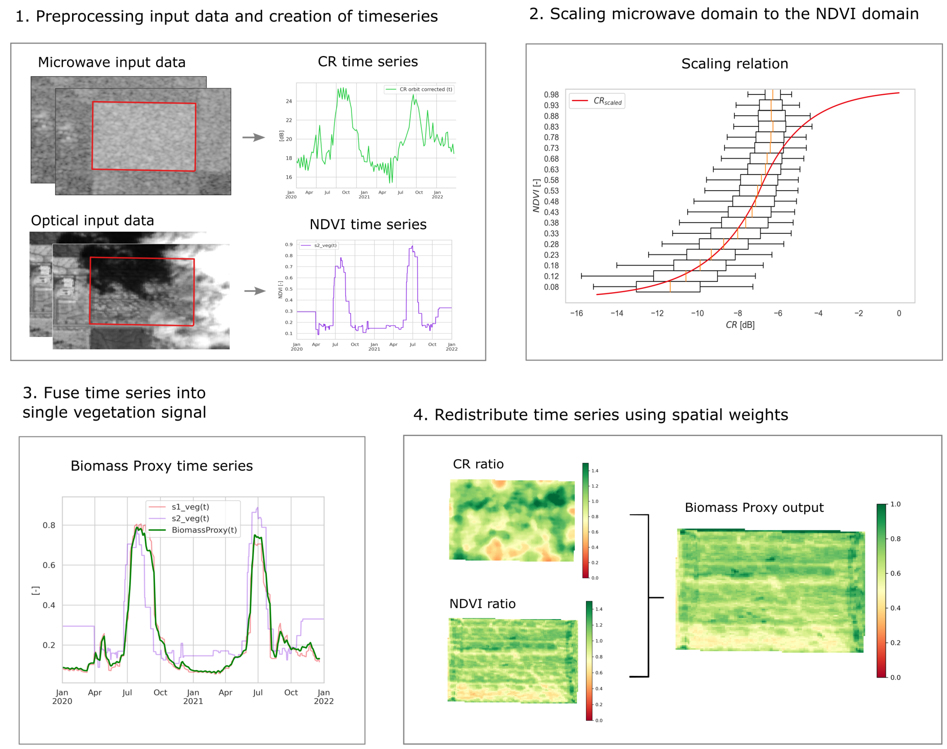
Temporal and spatial fusion happens separately in order to make use of different weighing strategies to leverage the different strengths of each signal in the two domains. The Biomass Proxy algorithm is designed to combine the strong temporal reliability of the radar signal with the high spatial resolution of optical data. The Biomass Proxy output therefore primarily reflects Sentinel-1 time series, while the spatial distribution is mostly reflected by Sentinel-2 patterns.
Figure 1. Overview of the methodology used to derive the Biomass Proxy. The input data, existing of microwave and optical data collected within field boundaries (marked by the red box), is run through several processing steps (1–4) to create daily Biomass Proxy output maps.
Remotesensing 16 00835 g001

2.2. Preprocessing Input Data and Creation of Time Series

2.2.1. Sentinel-1 Data

The Sentinel-1 mission [43] consisted of two satellites (Sentinel-1A and B) carrying a C-band (5.405 GHz) SAR system, providing dual-polarization imagery, i.e., backscatter coefficients in VV and VH polarizations, with a 10m spatial resolution over a 250 km swath. Each satellite revisits areas every 12 days, and using both satellites, coverage extends to 1–4 days over Europe and 6 days over the United States. Sentinel-1B stopped working in December 2021, but is soon to be replaced by Sentinel-1C, scheduled in 2024.
The radar signature of vegetated areas typically involves three elements: direct backscatter from the canopy, canopy-attenuated soil backscatter, and multiple scattering from vegetation–soil interactions [18,23,44]. For agricultural monitoring with Sentinel-1, it is essential to isolate the vegetation signal. VH polarization backscatter is more sensitive to volume scattering and vegetation, while VV polarization is responsive to surface scattering (Attema and Ulaby, 1978; Ulaby et al., 1981; [20]). CR, the ratio between VH and VV (Equation (1)), reduces the impact of factors like soil moisture and incidence angle, enhancing the radar’s ability to detect vegetation. Additionally, since radar backscatter is known to be impacted by speckle, a multi-temporal Lee sigma filter [45] and a median filter [46] are applied on the CR. An example of CR time series extracted from these spatially filtered CR images is presented in Figure 2.
C R = V H V V
The same location on earth can be viewed from different orbits. These relative orbits differ from one another in terms of incidence and azimuth angles. The backscatter coefficient generally decreases with increasing incidence angle; however, the subsequent impact on the CR depends on topography and geometry as well as vegetation structure [47]. As these characteristics may differ for each field, we derive the orbit correction factors (see Appendix A) over a fixed period of time (i.e., 2.5 years in the current version), and apply the correction on each orbit for each field individually, based on the relative differences in historical Sentinel-1 data characterizing the different orbits, to estimate the orbit-corrected C R o r b i t c o r r e c t e d ( t ) (Figure 2).

2.2.2. Sentinel 2 Data

The Sentinel-2 mission [48] comprises two satellites, Sentinel-2A (launched in 2015) and Sentinel-2B (launched in 2017). These satellites are equipped with the Sentinel-2 Multi-Spectral Instrument, which captures surface reflectance data across 13 spectral bands spanning the visible, near-infrared, and shortwave infrared ranges of the electromagnetic spectrum. With both satellites in operation, Sentinel-2 achieves a five-day revisit period.
To extract vegetation signals, the Biomass Proxy algorithm uses NDVI (Equation (2)) derived from surface reflectance measurements in the red (RED, Band4) and near-infrared (NIR, Band8) spectral domains at a 10 m spatial resolution. These domains are very sensitive to the vegetation photosynthetic activity; the leaf chlorophyll strongly absorbs red light for use in photosynthesis and the cell structure of the leaves, but on the other hand, it strongly reflects near-infrared light [49].
N D V I = N I R R E D N I R + R E D = B a n d 8 B a n d 4 B a n d 8 + B a n d 4
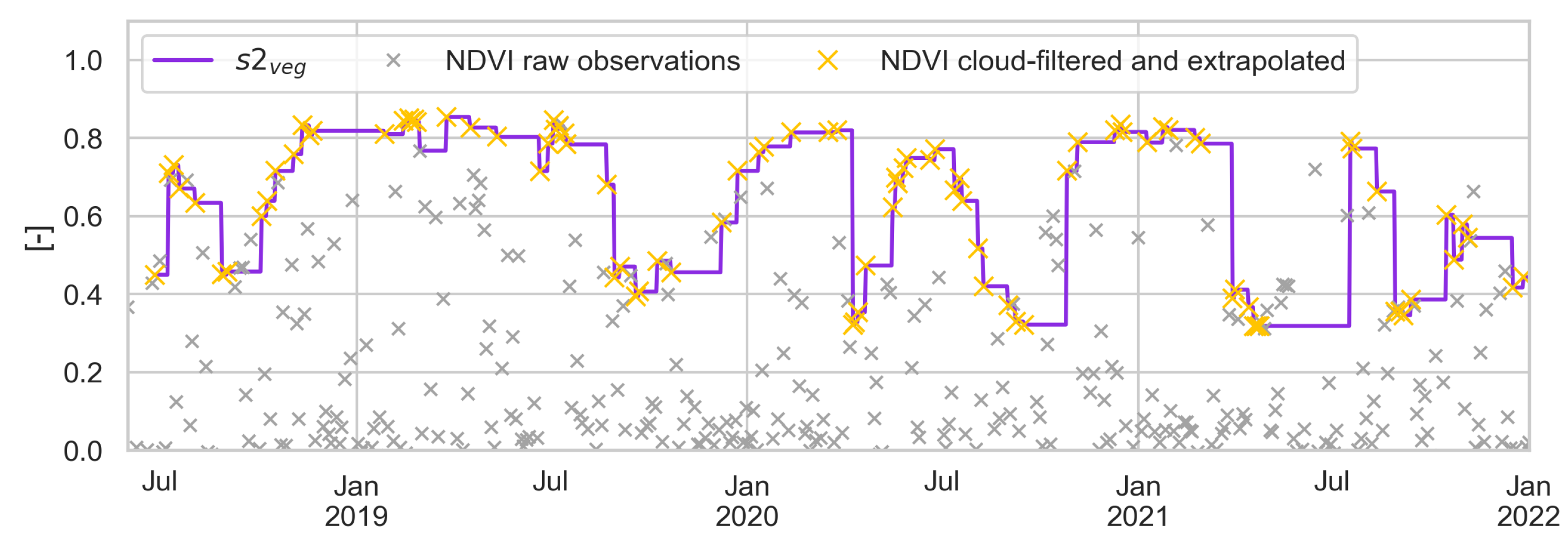
Preprocessing of optical data involves cloud masking the Sentinel-2 images by combining the Fmask [50], S2cloudless [51], and Sen2Cor [52] algorithms and snow and water masking by combining Fmask and Sen2cor. From the masked data, we create time series (Equation (3)) by extrapolating partially clouded images against the latest full coverage cloud-free image and then by front-filling the time series (Figure 3). Hereafter, the resulting time series is called s 2 v e g ( t ) . For deciding on the the most accurate representation of NDVI in the time series, our strategy is based on both the recency and cloud-free coverage of the image and follows a sigmoid decay function described by Equation (A2) in Appendix B.
s 2 v e g ( t ) = N D V I i if d w i ( t ) d w i n ( t ) N D V I n if d w i ( t ) < d w i n ( t )
where subscript i denotes the most recent image, and i n refers to any image before that.

2.3. Scaling CR to the NDVI Range

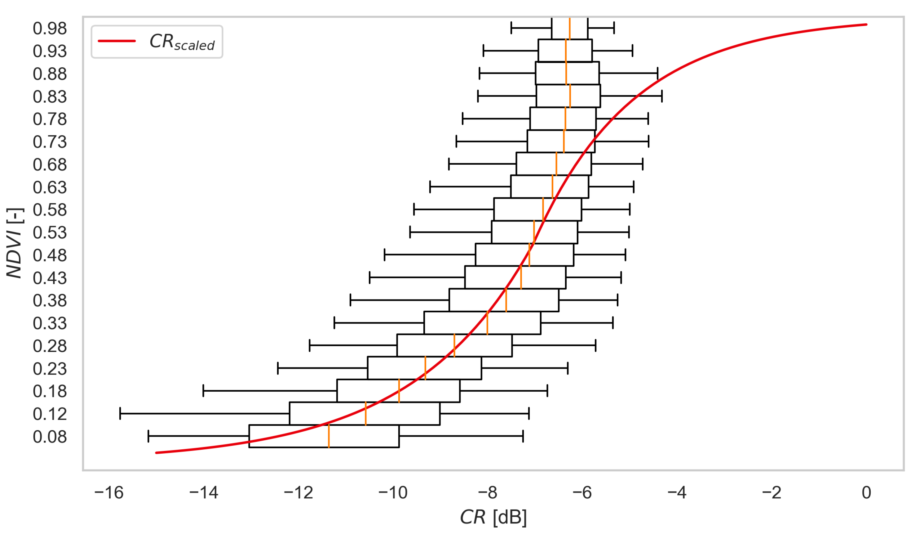
In order to fuse optical and radar vegetation signals in both time and space, we need both signals at comparable scales. We scale the radar signal to align with NDVI, since NDVI is a widely recognized and established optical vegetation index. The scaling function (Figure 4) is based on time series of CR and NDVI collected over more than a million fields spread all over the globe. The scaling function can be described as a combination of a power function, a linear center part, and an asymptotic tail (Equation (4)). The asymptotic shape was added for multiple reasons. Firstly, each CR value should be translatable, ensuring that a feasible translation exists for every CR value. Given that the upper limit of NDVI reaches one, the scaled values should not surpass this threshold. Secondly, stability within each domain is crucial for the algorithm. Relying solely on the power relation could lead to considerable fluctuations in radar values, an outcome we strive to circumvent. Lastly, the asymptotic shape of the process guarantees that an augmentation in the CR will consistently yield an increase in the scaled value, as opposed to capping the scaled value at one. The Pearson correlation coefficient r for the scaled CR ( C R s c a l e d ) is 0.62, and the Mean Absolute Error (MAE) is 0.16, suggesting the feasibility of scaling. However, it is noteworthy that the signals exhibit disparities, emphasizing that they should not be employed interchangeably (see Section 3).
C R s c a l e d = a · e ( b · C R + c ) + d if C R < C R linear m · C R + z if C R linear C R < C R asymptotic 1 1 k e n ( ( m · C R + z ) k ) if C R > = C R asymptotic
where C R s c a l e d is the result of scaling C R to an NDVI scale and a , b , c , d , m , z , n , k are empirical parameters derived by regressions using optical and radar observations over more than a million fields (See Appendix C). The result of applying scaling to the orbit-corrected CR time series ( C R s o ) is shown in Figure 5.
A custom weighed average considering up to 6 observations within the previous 24 days is applied to smooth the time series and is given by Equation (5). The resulting time series is called s 1 v e g ( t ) and is designed to eliminate noise in the CR signal without losing responsiveness to agricultural events.
s 1 v e g ( t ) = 1 W ( t ) i = N 1 w i ( t ) · C R s o ( t i )
where W ( t ) , the normalization factor, is defined as follows (Equation (6)):
W ( t ) = i = N 1 w i ( t )
where w i is the weight attributed to each CR value in a set of N scaled and orbit-corrected CR values { C R s o ( t n ) , C R s o ( t i ) , C R s o ( t 1 ) } , where n 6 and t t n < 24 days. In this context, subscript i denotes the nth image before t such that t 1 is the first image before time t. Then C R s o ( t 1 ) denotes the value of the scaled and orbit-corrected CR value of that image.
The weights are based on a Gaussian strategy (Equation (7)) proposed by Kitagawa et al. [53]. This strategy places emphasis on the most recent observation, positioning it as the central focus of the weighted averaging process.
g ( t t i ) = 1 2 π σ 2 · e ( t t i ) 2 2 σ 2
To further remove noise, we introduce a custom low-pass filter (Equation (8)) designed specifically to eliminate noise without introducing any significant delay. This filter is designed to operate solely on historical data, aligning with our objective of achieving near-real-time functionality.
b i = ( 1 | C R s o ( t i + 1 ) C R s o ( t i ) t i + 1 t i C R s o ( t i ) C R s o ( t i 1 ) t i t i 1 | + K )
Reducing delay is especially important after abrupt events such as harvest. To reduce delay after a harvest event, we introduce the Radar Harvest Detection Index ( R H D I ) (see Figure 5), which is greater than one when a harvest is likely occurring or has just occurred or equal to one otherwise. A high R H D I i increases the weight on the most recent observations, ensuring a timely response in the weighed average s 1 v e g ( t ) . This custom-built index is based on a number of indicators, including absolute value, slope, deflection, short-term averages, and long-term averages; see Appendix D. Combining the above-mentioned Gaussian strategy, low-pass filter, and radar harvest detection index (see Equation (9)) yields the weights used in Equation (5).
w i ( t ) = b i B ( t ) · g ( t t i ) G ( t ) · R H D I i R H D I ( t )
where the normalization factors G ( t ) , B ( t ) and R H D I ( t ) follow (Equations (10)–(12)):
G ( t ) = i = N 1 g ( t t i )
B ( t ) = i = N 1 b i
R H D I ( t ) = i = N 1 R H D I i

2.4. Fusing Time Series into Single Vegetation Signal

After the pre-processing and scaling processes, the NDVI and CR time series are fused using a combination of both static and dynamic weights. The static weights are equal for all fields globally and indicate the percentage of NDVI and scaled CR time series contributing to the fused temporal field average signal, respectively. Static weights offer the opportunity to adjust the individual contributions of each signal to shape the final vegetation signal.
Dynamic weights make sure that the most recent information is always leading. They are based on recency of the observation and the fraction of pixels covering the field. The latter can be less than one in case of cloud coverage or when the field is on a swath edge. The dynamic weights offer a consistent way to treat differences in overpass frequency over the globe for Sentinel-1 and Sentinel-2 satellites.
The static and dynamic weights together are used to calculate the relative contribution factors c o n t r i s 1 ( t ) and c o n t r i s 2 ( t ) of the spectral signals s 1 v e g ( t ) and s 2 v e g ( t ) , respectively, to the Biomass Proxy (Equations (13)–(15)).
B i o m a s s P r o x y ( t ) = 1 D i = 1 T ( s 1 v e g ( t ) · c o n t r i s 1 , T ( t ) + s 2 v e g ( t ) · c o n t r i s 2 , T ( t ) )
c o n t r i s 1 , T ( t ) = s w s 1 · c f s 1 ( t ) s w s 1 · c f s 1 ( t ) + s w s 2 · c f s 2 ( t )
c o n t r i s 2 , T ( t ) = s w s 2 · c f s 2 ( t ) s w s 1 · c f s 1 ( t ) + s w s 2 · c f s 2 ( t )
where c o n t r i s 1 , T ( t ) and c o n t r i s 2 , T ( t ) represent the contributions of both signals to the fusion process in the temporal domain (i.e., T), D the window of a small backward average (D = 5) to smooth the results of fusing the two signals, s w s 1 and s w s 2 the static weights of Sentinel-1 and Sentinel-2, and c f s 1 ( t ) and c f s 2 ( t ) the dynamic contributing factors (see Equations (16) and (17)).
c f s 1 ( t ) = 1 c f s 2 ( t )
c f s 2 ( t ) = 1 1 T i = 0 T d w s 1 ( t i ) d w s 2 ( t i ) + 1
where d w s 1 and d w s 2 are the dynamic weights for Sentinel-1 and Sentinel-2, respectively. The dynamic weights account for fluctuations in availability of input signals, due to prolonged cloud cover, or to low radar revisit frequency (see Appendix B for more details). While Biomass Proxy time series are largely based on CR, in the case of very low Sentinel-1 availability, the contribution of Sentinel-2 time series slightly increases. This is to ensure operational stability in low-radar-availability regions.

2.5. Redistributing Time Series Using Spatial Weights

To derive the Biomass Proxy maps for each day, the time series of field average fused product are downscaled to create Biomass Proxy pixel B i o m a s s P r o x y ( x , y , t ) values at 10 m resolution, the native resolution of Sentinel-2 (Equation (18)). Here, x, y, t represent the longitude and latitude of the field and acquisition date, respectively.
B i o m a s s P r o x y ( x , y , t ) = r a t i o ( x , y , t ) B i o m a s s P r o x y ( t )
The redistribution weights used in the downscaling process ( r a t i o ( x , y , t ) in Equation (19)) are made out of a combination of NDVI and scaled CR observations in the spatial domain.
r a t i o ( x , y , t ) = r a t i o s 1 , i ( x , y ) c o n t r i s 1 , S ( t ) + r a t i o s 2 , m ( x , y ) c o n t r i s 2 , S ( t )
where r a t i o s 1 , i ( x , y ) and r a t i o s 2 , m ( x , y ) represent the ratios between pixel values and the field average value of the respective image (in the case of NDVI, Equation (21)) or composite of images (in the case of CR, Equation (20)). Subscript m denotes the last full coverage cloud-free NDVI image. Images with any cloudy pixels are disregarded to prevent having any spatial artefacts from cloud-masking in the Biomass Proxy output maps.
r a t i o s 1 , i ( x , y ) = 1 N i = 1 N C R s c a l e d , i ( x , y ) C R s c a l e d , i
r a t i o s 2 , m ( x , y ) = N D V I m ( x , y ) N D V I m
With respect to Sentinel-1 images, we noticed (similarly to e.g., [54]) that the observed pattern is influenced by the incidence angle, whose effect was not spatially removed by the orbit correction. We therefore make a composite of the inner distributions of the latest six past images in the last 24 days (N ≤ 6). Here, C R s c a l e d ( x , y ) represents Sentinel-1 images that have been preprocessed and scaled with the scaling function described in Equation (4).
The contributions of the spectral signals in the spatial domain, c o n t r i s 1 , S ( t ) and c o n t r i s 2 , S ( t ) in Equation (19), follow the same fusion process as the temporal contributions (i.e., Equations (14)–(17)) and include static and dynamic weights. While Sentinel-2 NDVI is the main contributor to the spatial pattern through a high static weight, in cases of prolonged cloud cover, the dynamic weights make sure that the contribution of Sentinel-1 increases. In cloudy regions, a full coverage NDVI image may be weeks to months old and the radar component is used to fill the gaps despite a coarser spatial resolution after speckle filtering.
The dates of the most recent observations of Sentinel-1 and Sentinel-2 used in creating the daily Biomass Proxy maps are provided in the product metadata. Additionally, an overview of parameters currently used to process the Biomass Proxy can be found in Appendix E.

2.6. Selected Use Cases

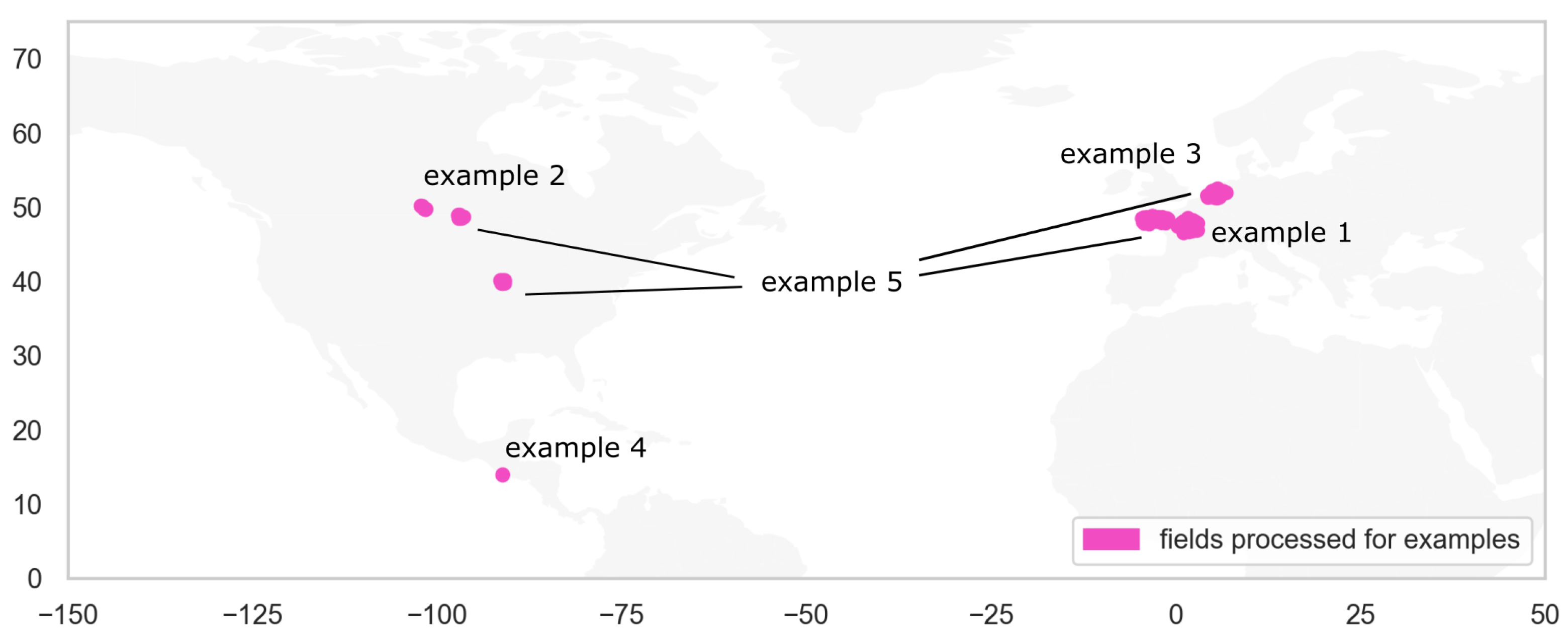
Since the launch of Sentinel-1 by the European Space Agency (ESA), SAR data have been increasingly used to monitor agricultural systems. Yet, radar applications mainly seem to remain in the realm of research, which could be explained by the relative complexity associated with the processing and interpretation of radar images compared to optical data [18,55]. Radar signals are under-leveraged, and can provide, next to their temporal reliability, key information of vegetation that is different from optical information. We will use several use cases to present and illustrate from a qualitative perspective the distinctive and novel insights provided by the fusion-based Biomass Proxy, which complement and extend beyond purely optical signals. The locations of the different use cases are given in Figure 6.
example 1:
To demonstrate the continuity of the Biomass Proxy under cloud cover, we selected two neighboring wheat fields in France, one of which was affected by prolonged cloud cover. We also demonstrate intermediate algorithm parameters and the dynamics of the algorithm.
example 2:
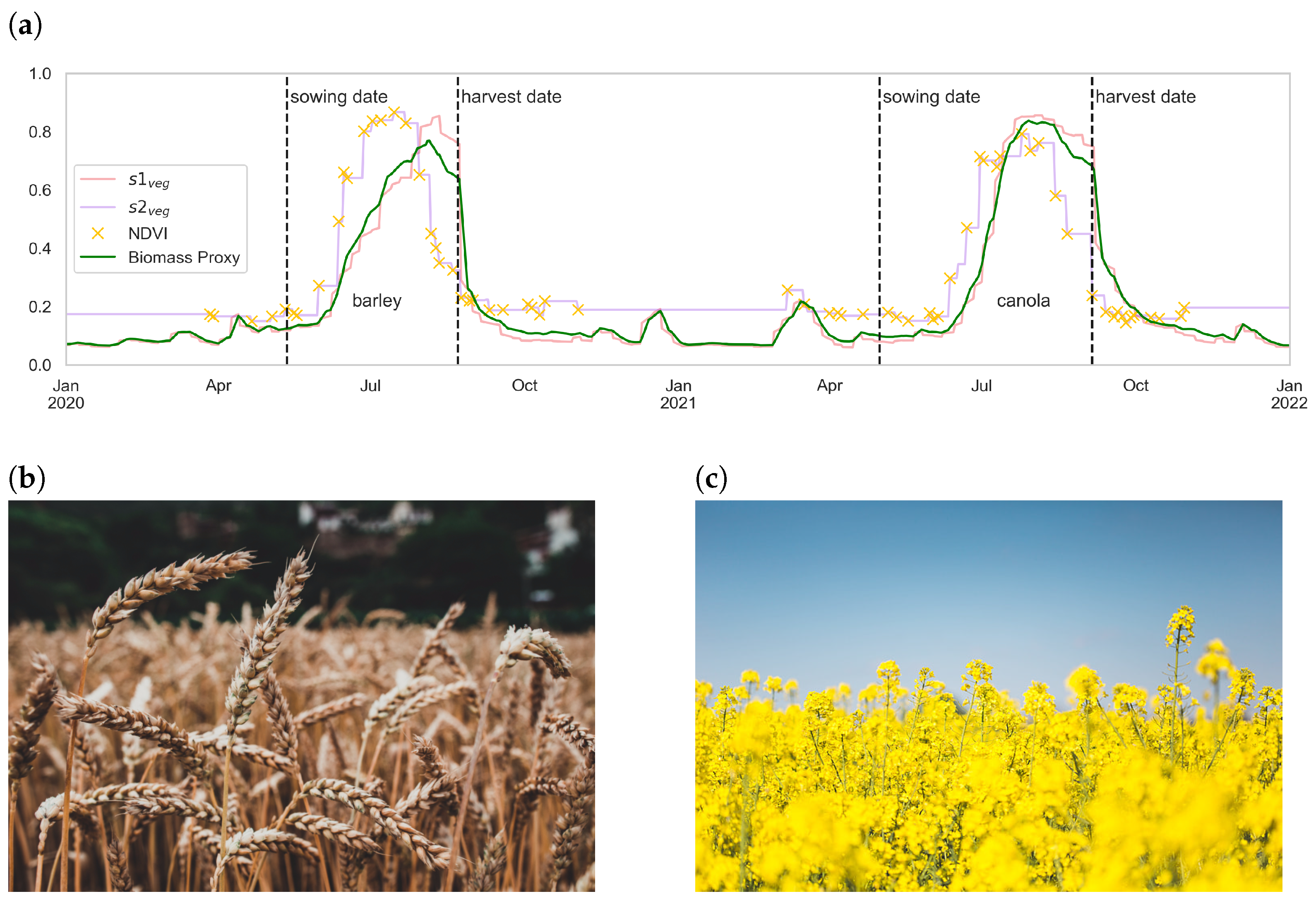
While the Biomass Proxy and NDVI can be similar, this example highlights observed differences between the Biomass Proxy and NDVI. We selected a field in Canada with barley and canola to show differences observed during flowering and senescence.
example 3:
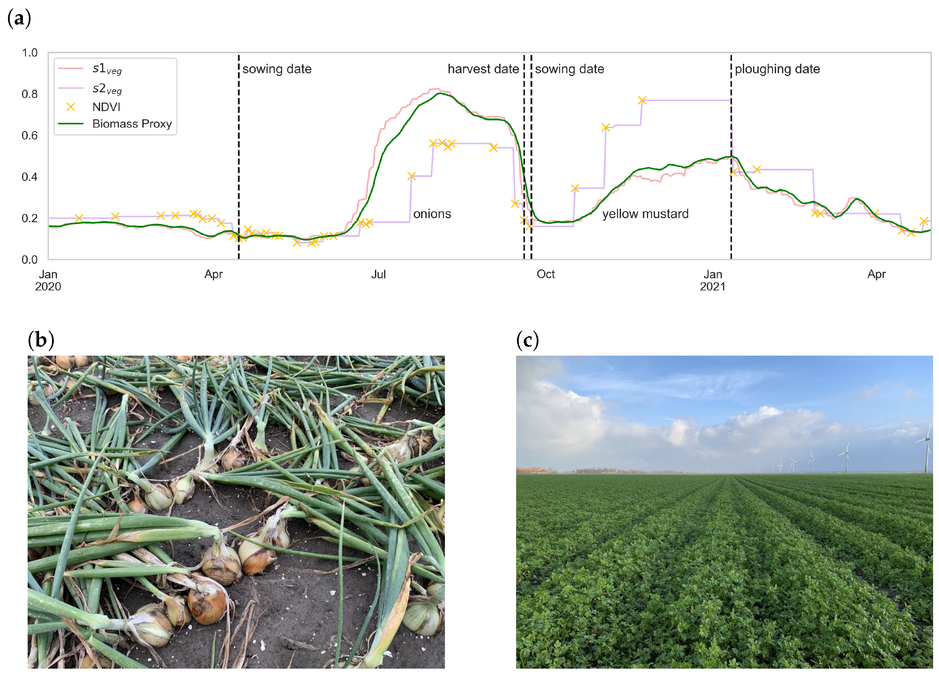
To illustrate variations and observed differences in signal ranges, we selected a field in the Netherlands cultivating onions and yellow mustard.
example 4:
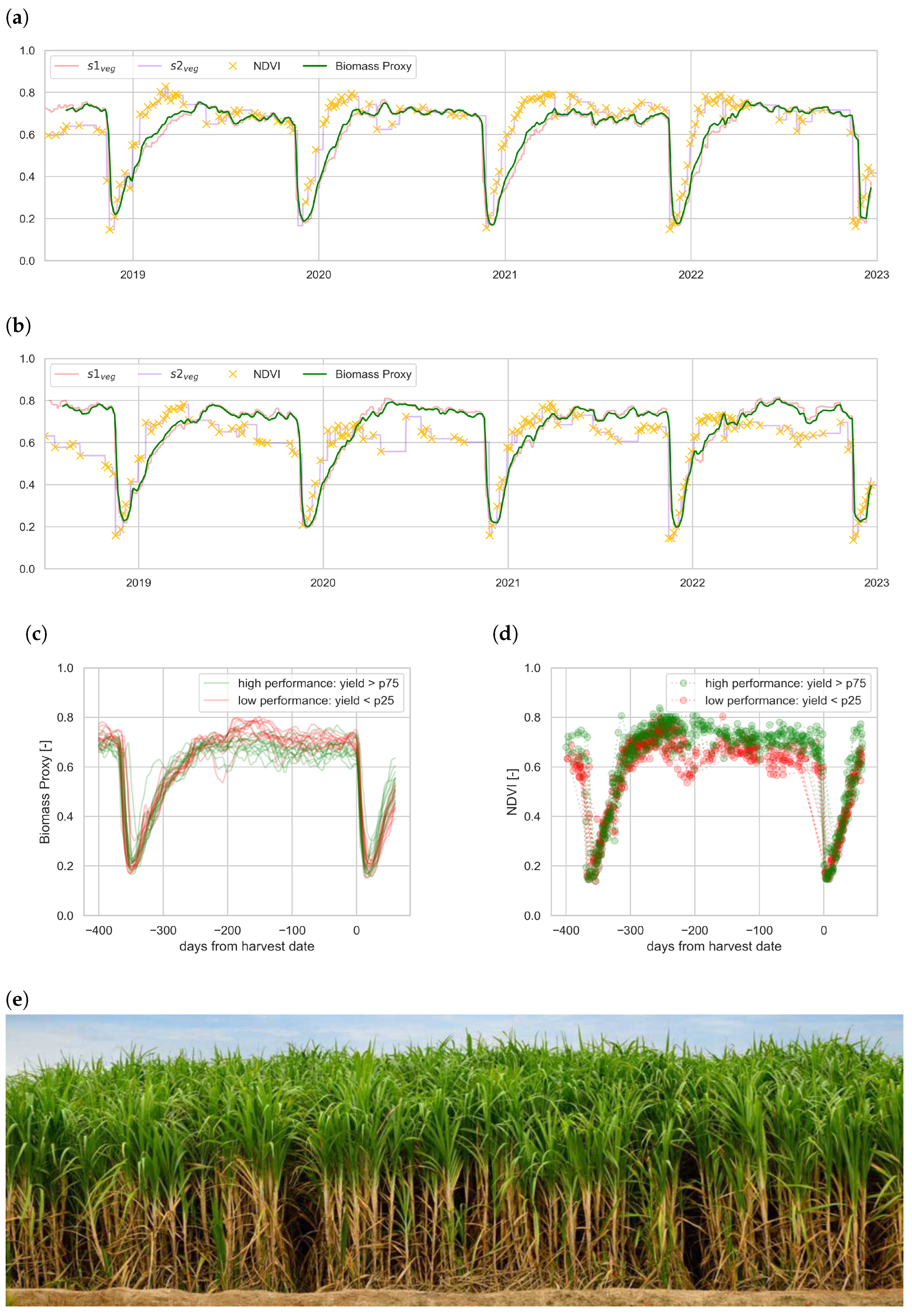
We illustrate the complementary value of Biomass Proxy and NDVI for sugarcane fields in Guatemala, in which we illustrate how the two indices respond differently to the build-up of sucrose.
example 5:
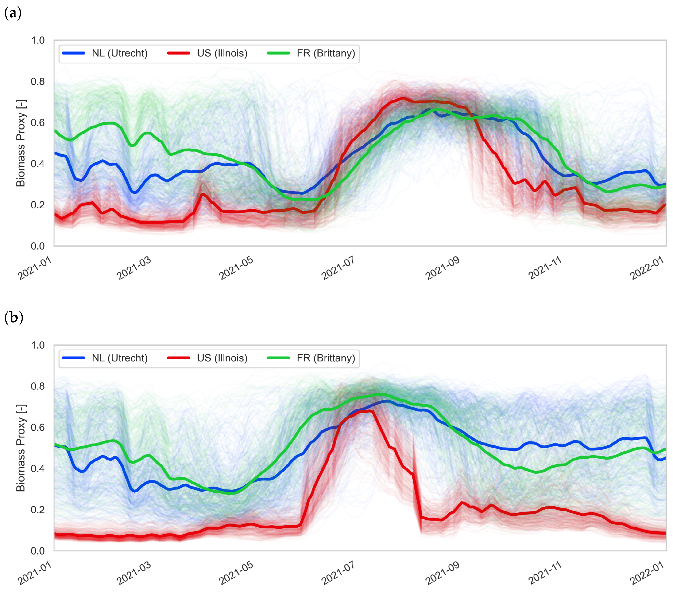
To demonstrate the global processing capabilities of the Biomass Proxy, we selected corn and wheat fields in different locations around the globe: France, the United States, and The Netherlands.

3. Results

3.1. Example 1: Biomass Proxy under Cloud Cover

The presence of clouds prevents reliable crop monitoring using optical remote sensing. The challenge of monitoring crops over cloudy regions is effectively addressed by the Biomass Proxy, whose time series primarily relies on SAR data. In this example, we demonstrate the ability of the Biomass Proxy to monitor crop growth in space and time in a continuous manner.
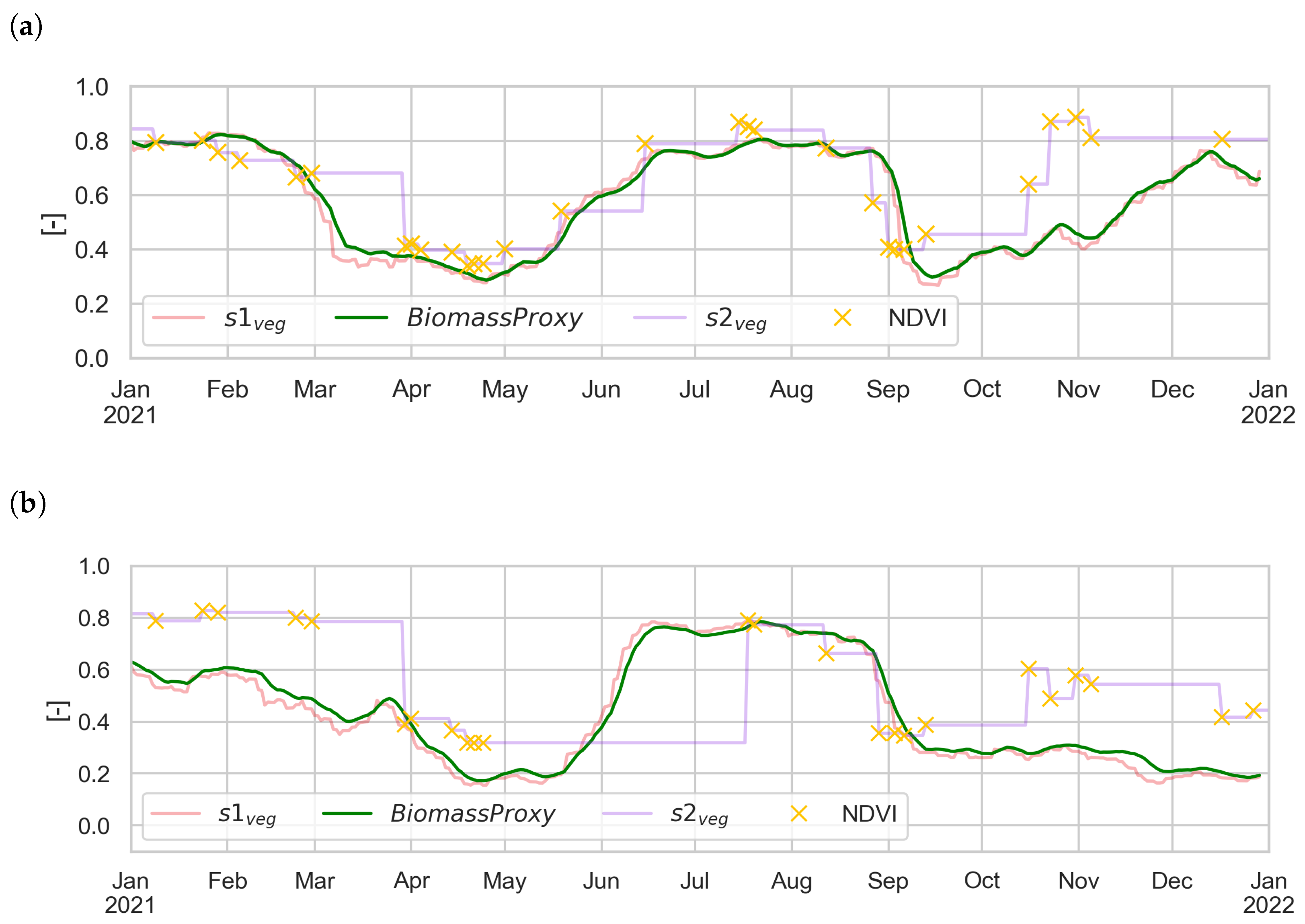
In Figure 7, we demonstrate the time series of the Biomass Proxy and intermediate algorithm parameters for two neighboring fields in France. Whereas the field represented in Figure 7a shows optical data updates in the order of weeks, a neighboring field (Figure 7b) was hindered by cloud cover throughout May, June, and July. The impact of clouds on the number of optical scenes available for the fusion process is clearly illustrated by the respective time series of the optical vegetation signal s 2 v e g ( t ) over the growing season of 2021. Due to the temporal fusion with s 1 v e g ( t ) , the impact of cloud coverage on the Biomass Proxy was reduced and the algorithm was able to provide a continuous vegetation signal.
This continuity is also provided in spatial maps for a 40 ha corn field (Figure 8). The daily Biomass Proxy images are a best estimate of the state of biomass in the field based on previous CR and NDVI distributions of Sentinel-1 and 2 images, which are also represented.
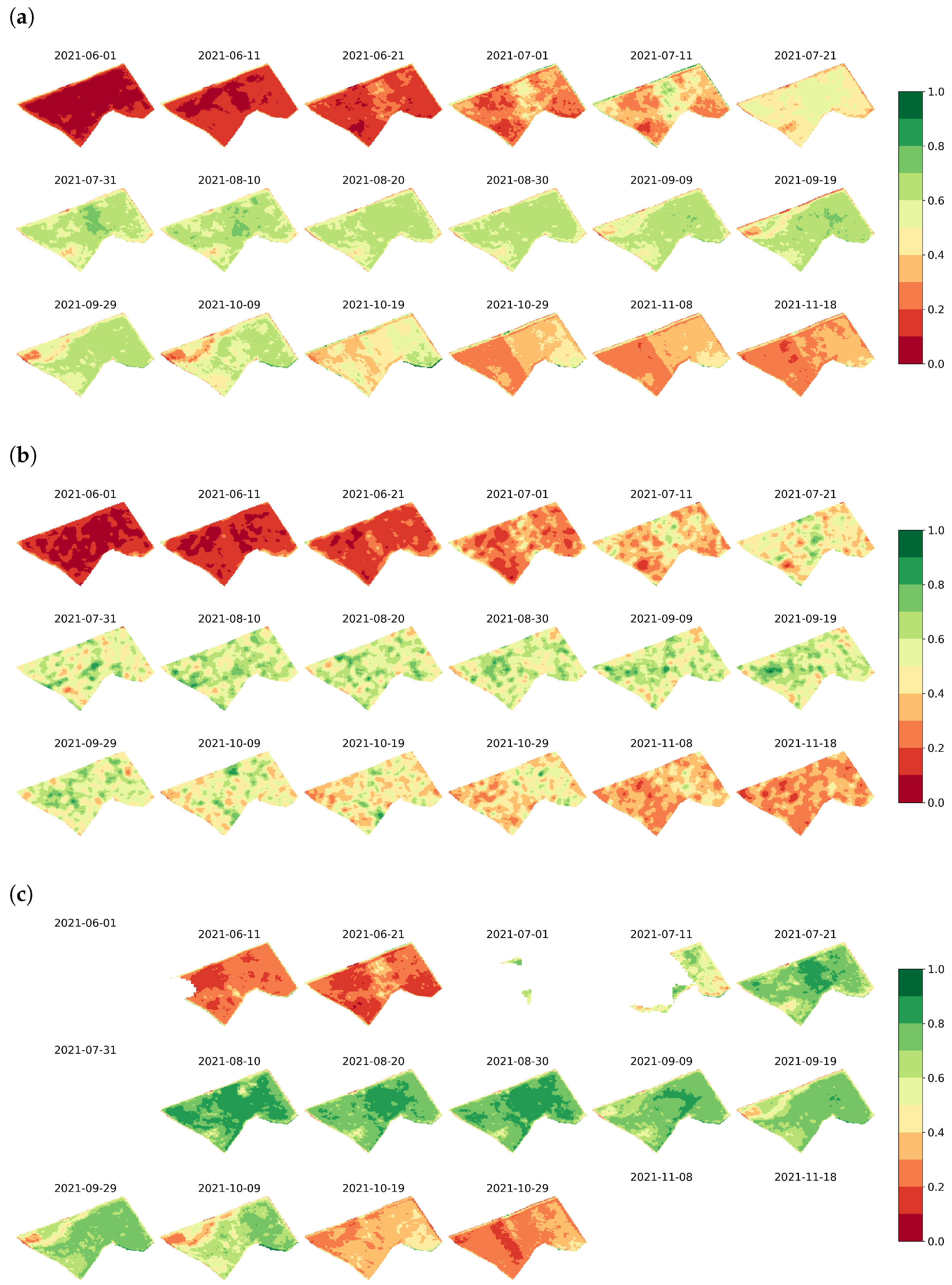
Biomass Proxy maps throughout the crop season over the same field are shown in Figure 9. To visualize the relative contributions of the spectral information, scaled CR composites and NDVI composites over the crop season are also shown in Figure 9b,c, respectively. It can be noticed that the field average Biomass Proxy primarily reflects the scaled CR average, while the spatial distribution is more dominated by NDVI patterns. Nonetheless, when no Sentinel-2 images are available for a long period of time, the CR composites gain in weight in the fusion process and help fill the gap.

3.2. Example 2: Biomass Proxy as an Indicator of Phenological Aspects

NDVI mainly represents the photosynthetic activity of leaves, which does not always correlate with the actual fresh biomass of the plant, especially during the senescence period. In this example, we illustrate the ability of the Biomass Proxy to describe relative changes in crop fresh biomass and differences we observed with NDVI time series. Time series of Biomass Proxy and NDVI observed over a field located in Saskatchewan, Canada cultivated with barley in 2020 and canola in 2021 clearly describe a strong decrease in NDVI during the senescence period, while the Biomass Proxy is slightly lessened before harvest (Figure 10).
In the case of barley, the decline in NDVI is explained by a change in color during the ripening stage. As the barley grains mature and reach full development, they undergo a color change from green to yellow-green, golden, and a light brown hue. NDVI responds naturally to a color change, which corresponds with an increasing amount of red light being reflected. NDVI observed over this field decreases and loses about 80% of its initial value in the process. During the ripening and senescence phases, barley fresh biomass does diminish before harvest, but at a much slower rate than the density of green leaves [56]. Barley plants redirect nutrients from vegetative parts (leaves, stems) to the developing grains. As a result, the plant begins to dry out, and the reduction in plant water content leads to a decrease in the overall plant weight. Barley can lose around 20% of its initial weight in the process [56]. Being sensitive to plant water content, the Biomass Proxy shows a similar decrease. It provides slightly different but complementary information than NDVI, which may be useful for crop management.
For canola crops, a color change occurs during flowering, temporarily transitioning the canopy upper layer to a yellow hue. As canola matures and the leaves start to dry and change color from green to yellow (and eventually brown during senescence), there is a shift in the spectral reflectance properties, leading to a strong decrease in NDVI. As for barley crops, the fresh biomass of canola plant and the associated observed Biomass Proxy decrease during the senescence period, but at a much slower rate than NDVI (Figure 10). Based on field data, Malhi et al. [57] observed a similar slow decrease in canola biomass three months after seeding, further confirming the close correlation between the Biomass Proxy and fresh biomass.

3.3. Example 3: Differences between Biomass Proxy and NDVI Absolute Values

The scaling relationship (Section 2.3) demonstrated that NDVI and Biomass Proxy time series are correlated, but it also highlighted the presence of variability. We have seen in previous examples that observed differences between Biomass Proxy and NDVI may be related to phenological stages, but there are also differences in the absolute value ranges. This example illustrates such distinctions for a field located in Flevoland, The Netherlands, which cultivated onions as the main crop in summer 2020, followed by yellow mustard as a winter cover crop. In fact, the Biomass Proxy of onions was much higher than that of yellow mustard throughout the crop season (Figure 11). The opposite effect is observed for NDVI, which reaches higher values for yellow mustard than onions.
Observed differences in the remote sensing indices may be partly due to differences in the canopy structure of the onions and yellow mustard (Figure 11). Onions have relatively narrow leaves and form a relatively open canopy, while the yellow mustard plants consist of large broad leaves that fully cover the underlying soil and are associated with greater canopy light interception and therefore higher NDVI values than onions. In contrast, the Biomass Proxy is higher for onions than for yellow mustard and observed differences may be associated with a variety of factors, such as plant structure and water content.
Conjointly, yields were much higher for onions (57 t/ha) than for yellow mustard (5 t/ha). It should be noted that onion biomass and water content are mainly concentrated in the bulb. Since the bulbs started to surface at the end of July and were almost completely above soil in August (see Figure 11b), this could possibly be an explanation for the observed higher values.
An alternative rationale for the difference could stem from the distinct scattering mechanisms of radar regarding to vegetation structure. For instance, in broadleaf crops like yellow mustard, radar attenuation happens primarily through direct surface scattering. Conversely, in crops like onions with their vertically elongated leaves, radar is predominantly affected by volume scattering [58]. Another possible source of uncertainty for differences observed is radar–soil interaction; however, we did not identify any consistent response of soil influence in the final product signal in the various use cases we investigated.
This example clearly showed that the Biomass Proxy provides additional information to NDVI observations. However, the interpretation of the differences between Biomass Proxy and NDVI may be complex and crop-dependent. Further research is needed to fully characterize differences between NDVI and the Biomass Proxy for various crops.

3.4. Example 4: Biomass Proxy and NDVI Time Series and Their Complementary Value

The fact that temporal profiles of NDVI and Biomass Proxy may differ and represent various aspects of crops is a feature that may be useful to refine crop classification and facilitate in-season crop monitoring. In this example, we demonstrate the complementary value between NDVI and Biomass Proxy signals to monitor sucrose content. Observations over multiple sugarcane seasons and fields in Guatemala are used to illustrate the opposite response of Biomass Proxy and NDVI products to changes in sucrose content (Figure 12). Such differences can be leveraged to better assess sucrose yield.
Around 200 days pre-harvest, both NDVI and Biomass Proxy time series of sugarcane with low or high levels of sucrose, respectively, start diverging, making possible to discriminate between low and high yields. One would expect that time series correlating with higher yields would exhibit an upward trajectory, a phenomenon indeed observable in the NDVI time series. However, an interesting pattern emerges in the Biomass Proxy time series, wherein contrary behavior is observed.
High-performance seasons exhibit lower Biomass Proxy values pre-harvest compared to low-performance seasons. This phenomenon was first discovered in Mozambique by den Besten et al. in [27] and further investigated in [59]. The authors found that the CR responds to the development of sucrose accumulation, which changes the internal distribution of sucrose and vegetation water in the stalk. The observed backscatter decreases when sucrose accumulated in the sugarcane stalk and water content decreased. We find similar results for the Biomass Proxy in Guatemala.
The divergence between NDVI and the Biomass Proxy aids in differentiating high-yield (high NDVI, low Biomass Proxy) from low-yield seasons (low NDVI, high Biomass Proxy) relatively early on in sugarcane fields, which can possibly be leveraged in predicting sucrose yield. This example illustrated that complementary use of NDVI and the Biomass Proxy has potential to be utilized in field performance assessment.

3.5. Example 5: Biomass Proxy Time Series in Various Geographic Regions

Previous use cases focused on the analysis of individual fields, highlighting specific features of the Biomass Proxy. Here, we want to demonstrate Planet capability to provide consistent products globally and the benefit for large-scale agricultural applications. Figure 13 shows time series of 1000 maize fields and 1000 wheat fields located in specific regions in the Netherlands (NL), France (FR), and the United States (US) to characterize differences in cropping seasons.
Maize typically grows from April–May to September–October in Europe and can be harvested late in November in France [60]. Biomass Proxy time series of fields located in NL and FR show an increase around mid-June. This increase corresponds to the expected peak of growth two months after planting [20], a period with significant stem elongation and leaf growth. Then, as it reaches flowering, the amount of water in the crop remains relatively stable [21], as does the height [61], until the plant matures and starts drying. Figure 13 clearly illustrates the difference in growing season timing between the different countries, especially early harvest dates in the US, compared to NL and FR.
A similar analysis has been conducted for wheat fields located in the same regions (Figure 13b). There are clear differences between Europe and US time series in terms of signal amplitude and variability, especially after harvest, and crop season length. Typically, spring wheat is planted in mid-February to mid-June in Europe and April–May in the US, and it is harvested in July in France and in August in Illinois, US. However, due to high precipitation in July 2021, harvest started mid-August in Brittany, France and the Netherlands. Unlike US fields, where Biomass Proxy time series fell rapidly after harvest, we observed that the Biomass Proxy of fields located in FR and NL slowly decreases after harvest due to stubble, straw, and crop residue that remains in the field, depending on the use of tilling or plowing practices used after harvest.
The observed differences clearly describe different farming practices that exist between Europe and the US. In Europe for instance, crop seasons are more often alternated with winter cover crops [62], and crop residue is left on the surface after harvest, while farmers in Illinois, US, do not generally plant cover crops due to time or cost constraints [63] and leave their fields bare between consecutive seasons. Consequently, the slopes of the Biomass Proxy time series after mid-August are more representative of post-harvest practices than crop senescence.
This example highlighted that the global processing capabilities of the Biomass Proxy provide the potential to analyze regional differences in crop practices. The Biomass Proxy can be used to derive insights ranging from the intra-field scale to the national scale.

4. Discussion

The Biomass Proxy fuses the temporal continuity of Sentinel-1 SAR with the spatial resolution of Sentinel-2 optical imagery. Biomass Proxy time series greatly benefit from the ability of SAR to penetrate clouds. This alleviates the challenge of monitoring crops under cloudy conditions (see Section 3.1), especially for crops with short phenological cycles (e.g., canola; see Section 3.2), and significantly improves event detection, such as harvests (see Section 3.2). Biomass Proxy time series can differ from NDVI during distinct phenological phases, which may aid in characterizing phenological aspects. Differences between the Biomass Proxy and NDVI (see Section 3.2 and Section 3.3) may also offer opportunities for early crop classification and can also help to assess field performance (see Section 3.4). All these opportunities can be seized in any location where Sentinel-1 and Sentinel-2 data are available. The Biomass Proxy is produced uniformly across the globe and comparing crops for various regions can even provide insights into regional cropping patterns (see Section 3.5).
While the study has provided valuable insights into potential use cases, it is important to raise some discussion about the current open questions and potential limitations of the methodology. Even though the use of SAR observably enhanced the vegetation dynamics in cloudy conditions, the high spatial resolution of the Biomass Proxy still mostly relies on optical data because SAR spatial data, despite filtering, are impacted by speckle interference. Therefore, cloud-free optical observations are needed to accurately capture dynamics at the intra-field scale (see Section 3.1). To increase the temporal coverage of radar and optical observations, further work will include extending the Biomass Proxy framework to other optical sources (e.g., PlanetScope, Landsat) and future high-resolution SAR imagery (e.g., Sentinel-1C and -1D [64], NISAR [65], ROSE-L [66]).
Fusing the strengths of SAR and optical imagery may offer many opportunities and such a fusion process was made possible by the use of a scaling relationship (see Section 2.3) between CR and NDVI. We found CR and NDVI to act similar in the crop vegetative phase; however, significant differences between NDVI and CR were observed during the plant senescence of specific crops (see Section 3.2) and might affect the performance of the scaling function when bringing together temporal and spatial domains (see Section 3.2, Section 3.3 and Section 3.4). Therefore, further research is needed to evaluate the benefit of using different optical vegetation indices which might be more directly linked to what is observed by the radar vegetation signal. These may include Short Wave InfraRed (SWIR) bands, as they may be suitable given their sensitivity to plant water content [67,68].
While the product has shown potentially valuable traits, naturally, a much wider validation effort is required to assess the consistencies of these characteristics at a global scale. While our demonstration studies (see Section 3.1, Section 3.2, Section 3.3, Section 3.4 and Section 3.5) various crops in various regions and climates, we have only begun to explore the extensive possibilities in crop analysis. Numerous potential applications for diverse crops, spanning field performance, crop management strategies, environmental events, pests, diseases, irrigation, and beyond, could exist. A comprehensive research effort is imperative to uncover the full spectrum of opportunities for the product, especially when used in conjunction with other indices, within the domain of agricultural monitoring.
Future work will also have to investigate the relations between the Biomass Proxy and the crop fresh biomass and yield. A preliminary study showed high correlations (r2 around 0.9) between Biomass Proxy and fresh biomass of maize through the growing season [69]. However, the link between the Biomass Proxy and absolute values of crop biomass will have to be derived on a per-crop basis and will require a dedicated effort.

5. Conclusions

Released in May 2023, Planet’s Biomass Proxy product offers a timely, accessible, and analysis-ready product indicative of above-ground crop biomass dynamics at 10 m spatial resolution. Based on Earth observations from Sentinel-1 and Sentinel-2 constellations, the Biomass Proxy is a cloud-free vegetation monitoring product for agriculture management at scales varying from the intra-field scale to the national scale. In this paper, we described the processing algorithm and illustrated the main attributes of the Biomass Proxy product. The algorithm combines the strong temporal reliability of the radar signal with the high spatial resolution of optical data in a simple analytical fusion process. The Biomass Proxy does not fundamentally represent a cloud-free NDVI product, but rather a radar-based vegetation index that is more correlated to the plant water content and fresh biomass than the density of green leaves. In fact, the complementary value between the radar and optical data raises opportunities for agricultural applications, such as crop classification, field performance assessment, phenological stage monitoring, and yield forecasting. We have demonstrated that Biomass Proxy can be a valuable tool for crop management, particularly in cloudy regions where other remote sensing solutions are scarce or at coarse resolution. Sensitive to the plant water content, the Biomass Proxy is expected to support crop management, mitigate the effects of climate variability on agriculture, and provide accurate information on plant growth status and environmental stresses.

Author Contributions

Conceptualization, R.B. and B.A.; methodology, R.B. and B.A; software, R.B., B.A., F.C., T.v.d.H., R.K.; validation, R.B., N.d.B., P.G., D.J., M.R. and G.R.; formal analysis, R.B.; investigation, R.B.; data curation, R.B. and N.d.B.; writing—original draft preparation, R.B. and N.d.B.; writing—review and editing, B.A., N.d.B. and P.G.; visualization, R.B.; supervision, B.A. and R.d.J.; project administration, R.B., B.A. and A.Z.; All authors have read and agreed to the published version of the manuscript.

Funding

This research received no external funding.

Institutional Review Board Statement

Not applicable.

Informed Consent Statement

Not applicable.

Data Availability Statement

The data presented in this study are available on request from the corresponding author. Due to privacy restrictions associated with the presented use-cases, they are not publicly shared. An open dataset of the Biomass Proxy can be found in https://collections.sentinel-hub.com/crop-biomass (accessed on 27 February 2024).

Acknowledgments

The authors would like to express their gratitude to those operating and building the infrastructure that supports running the Biomass Proxy algorithm. Furthermore, the authors express their gratitude for the in situ data that were provided in support of the use-cases presented. Moreover, it should be noted that the findings and views described herein do not necessarily reflect those of Planet Labs PBC.

Conflicts of Interest

All authors were employed by the company Planet Labs PBC.

Abbreviations

The following abbreviations are used in this manuscript:
MDPIMultidisciplinary Digital Publishing Institute
DOAJDirectory of open-access journals
NDVINormalized Difference Vegetation Index
CRCross Ratio
ARDAnalysis-Ready Data
SARSynthethic Aperture Radar
VHVertically Emitted–Horizontally Received backscatter
VVVertically Emitted–Vertically Received backscatter

Appendix A. Sentinel-1 Orbit Correction
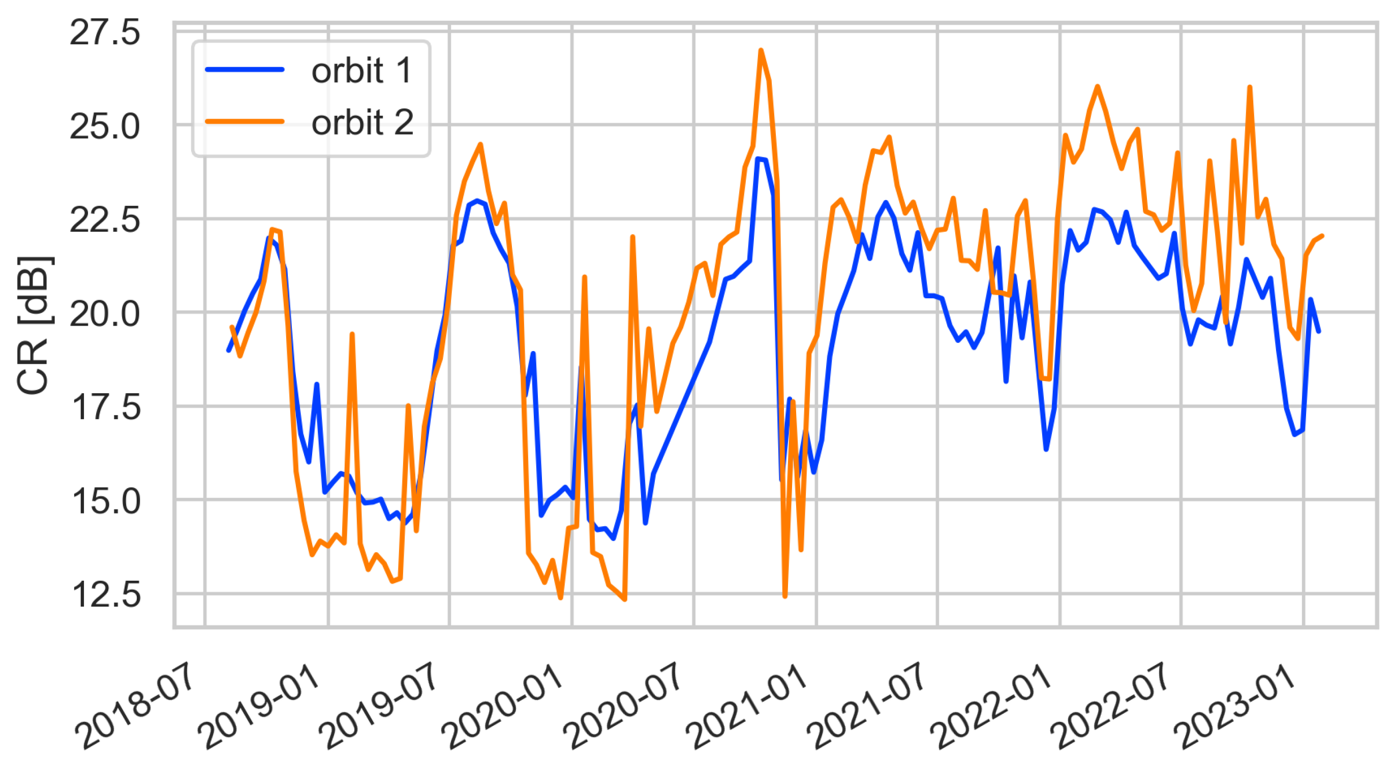
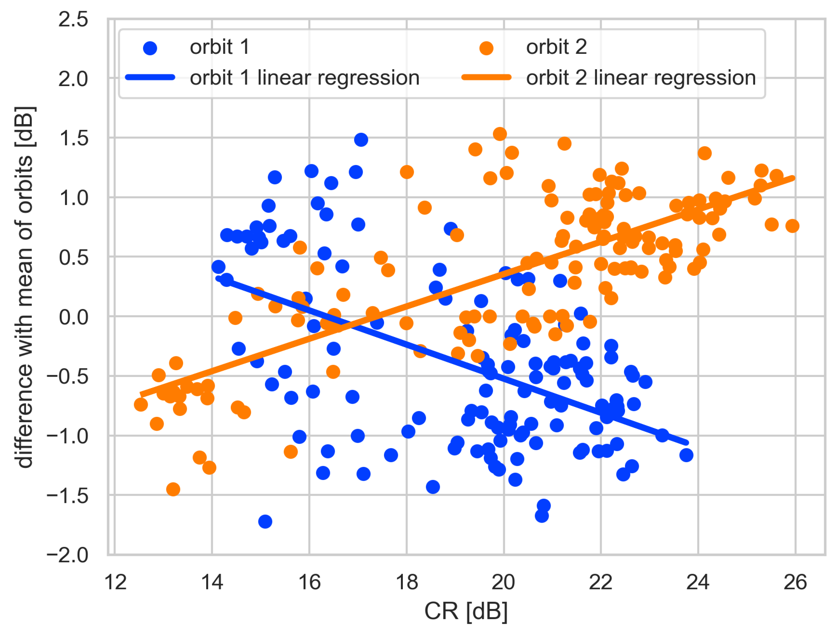
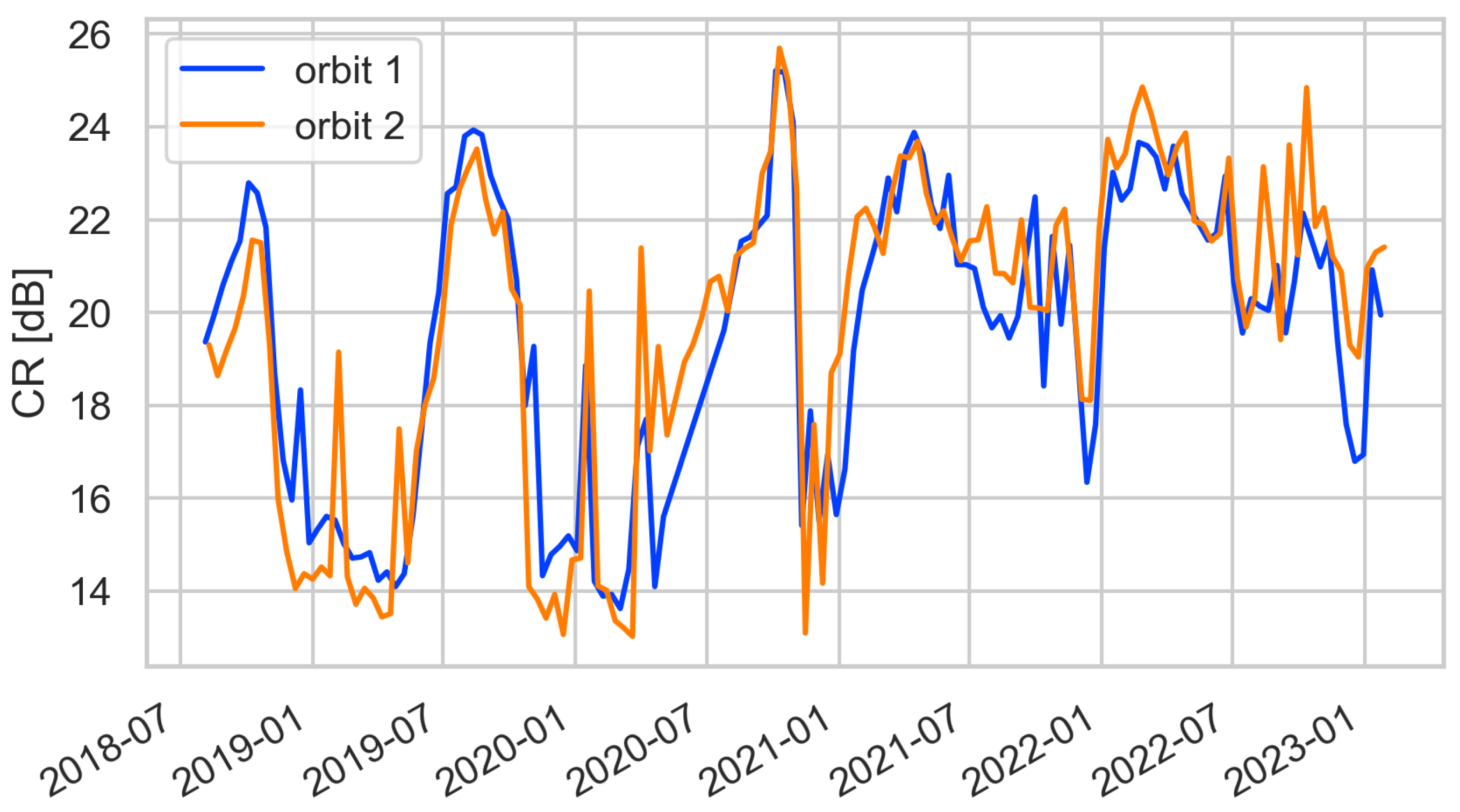
The relative orbit delineates the trajectory followed by each Sentinel-1 satellite as it traverses a specific region. Images captured along the same relative orbit share identical incidence angles and azimuth. As incidence angle and azimuth may impact the observed backscatter, we apply orbit correction per field (Equation (A1)) over past Sentinel-1 observations. Figure A1, Figure A2 and Figure A3 demonstrate the process of orbit correction for an example field with only two relative orbits. We take the separate orbits of the Sentinel-1 CR (Figure A1) and calculate the distance of the rolling mean (centered, 25 days) of the orbit to the rolling mean of all orbits and apply a linear regression over that difference (Figure A2). The derived regression parameters are implemented on the separate orbits (Figure A3).
C R o r b i t c o r r e c t e d , o r b i t x ( t ) = ( 1 A o r b i t x ) · C R o r b i t x ( t ) + B o r b i t x
where x is the number of the relative orbit and A x and B x regression coefficients corresponding to the linear regression between the CR of orbit x and the difference with the mean of orbits (Figure A2).
Figure A1. The Sentinel-1 CR for two different relative orbits.
Remotesensing 16 00835 g0a1
Figure A2. Linear regression of the distance to the mean of the orbits of Figure A1, with, in this case, Pearson r = −0.51 and r = 0.76 for orbits 1 and 2, respectively.
Remotesensing 16 00835 g0a2
Figure A3. The Sentinel-1 CR after the orbit correction.
Remotesensing 16 00835 g0a3

Appendix B. Dynamic Weight

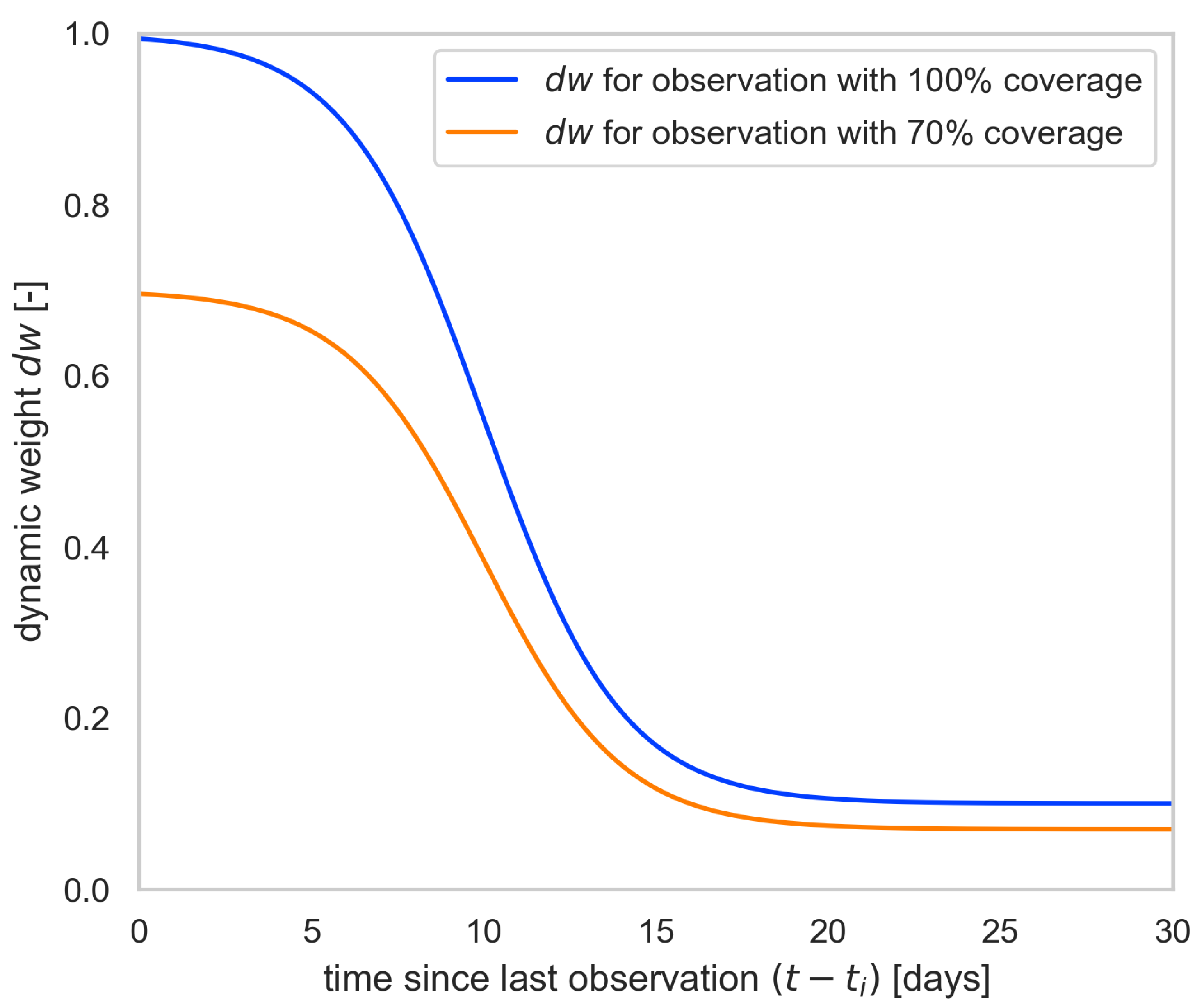
The dynamic weight function has been developed to facilitate decision-making processes by evaluating the reliability and accuracy of an image in portraying the current situation in the field. This assessment is based on two primary factors: the age of the image and its coverage. As an image ages, the certainty of its ability to accurately represent the present diminishes, and reduced spatial coverage further amplifies uncertainty. This is to be reflected in an S-shaped function. The dynamic weight function assigns high values to recent images (within a week) and subsequently diminishes rapidly. To illustrate how this can be interpreted, consider the following example. An image with 50% coverage of the present is deemed more credible than a fully covered image from two weeks prior. The function asymptotically approaches a low but stable contribution.
d w ( t ) = c o v e r a g e i 1 v 1 1 1 + e δ 1 1 + e β ( t t i ) + δ 1 1 + e δ
with t the current date and t i the date of the last observation, β and δ decay exponents, and v the vertical range to decay. The values are given in Table A1.
Table A1. Decay function constants.
ConstantValueUnit
v0.9-
β 0.5-
δ 5days
Figure A4. Dynamic weight illustration.
Remotesensing 16 00835 g0a4

Appendix C. Scaling Parameters

C R s c a l e d is the result of scaling C R to an NDVI scale and a , b , c , d , m , z , n , k are empirical parameters derived by regressions over more than a million fields. They are given in Table A2. These are mathematical parameters to ensure the form of the scaling function.
The empirical parameters (from Equation (4)) of the power function and linear function a , b , c , d , m , z were estimated by using non-linear Orthogonal Distance Regression [70] on time series of C R and s 2 v e g worldwide, where d w s 2 (see Appendix B) is above 0.85 and with a uniform sample size for each bin of 0.05 NDVI. The asymptotic function with parameters n , k was added by design.
Table A2. Regression parameters used in Equation (4).
ParameterValue
a0.99 ×   10 11
b3.96 ×   10 01
c27.4
d1.78 ×   10 02
m1.91 ×   10 01
z1.845
n2.50
k5.00 ×   10 01

Appendix D. Radar Harvest Detection Index

The radar harvest detection index is designed to put emphasis on the most recent observation in case of a harvest occurring or right after. Older images are not representative anymore in the situation of an harvest. It was not designed to obtain an exact date of harvest; there may not even be an observation on the harvest date. The determination of parameters was achieved through a systematic exploration employing trial and error methodologies. It contains many empirical factors but has shown, however, to be remarkably effective in detecting harvest events.
The design combines many factors, as the harvest can occur in different forms in the time series. A weighed average of the combination of these indicators is what we call the radar harvest detection index and is given by Equation (A3).
R H D I i = Y i 1 + H 1 · C R s o ( t i ) if Y i > H 2 1 if Y i H 2 Y i = K 9 P x = 1 8 ( F x K x ) + K 10 Y i K 9 P = x = 1 8 K x
The factors F x contributing to the weighted average are given through Equations (A4)–(A11)
F 1 = C 1 C R s o ( t i ) + C 2 C 3
F 2 = G A i ( σ 2 ) + C 4 C R s o ( t i ) + C 4 C 5
F 3 = C R s o ( t i 1 ) C R s o ( t i ) C 6 ( t i t i 1 + C 7 )
F 4 = G A i ( σ 1 ) C R s o ( t i 1 ) T A i ( σ 1 ) C 8
F 5 = G A i ( σ 2 ) C R s o ( t i ) C 9
F 6 = U A i C R s o ( t i ) C 10 C R s o ( t i ) C 11
F 7 = G A ( σ 2 ) C R s o ( t i ) + C 12 C R s o ( t i ) C R s o ( t i 1 ) + C 12 if G A ( σ 2 ) C R s o ( t i ) > 0 C R s o ( t i ) C R s o ( t i 1 ) 0 0 else
F 8 = ( G A ( σ 2 ) C R s o ( t i ) ) ( C R s o ( t i 1 ) C R s o ( t i ) + C 13 ) C 13 if G A ( σ 2 ) C R s o ( t i ) > 0 C R s o ( t i ) C R s o ( t i 1 ) < 0 0 else
The weighing factors are based on averages and Gaussian averages (Equations (A12) and (A13)) of the scaled and corrected Cross Ratio values C R s o in a set of values defined by S i = { C R s o ( t i 2 ) C R s o ( t i n ) } , where n is such that t i 1 t i n 60 days. The subscript i denotes the image for which the R H D I i is calculated.
G A i ( σ ) = 1 G i ( σ ) n = 2 | S i | g ( t i 1 t i n , σ ) C R s o ( t i n ) T A i ( σ ) = 1 G i ( σ ) n = 2 | S i | g ( t i 1 t i n , σ ) t i n U A i = 1 | S i | 2 n = 2 | S i | C R s o ( t i n )
g ( t i 1 t i n , σ ) = 1 2 π σ 2 · e ( t i 1 t i n ) 2 2 σ 2 G i ( σ ) = n = 2 | L S i | g ( t i 1 t i n )
The constants used in the calculation of R H D I are listed in Table A3.
Table A3. Constants used in calculation of the R H D I .
ParameterValue
H13
H25.5
K12
K21
K31
K41
K52
K66
K71
K81
K98
K101
C13
C20.7
C33
C40.25
C51
C60.075
C73
C80.05
C90.3
C100.3
C110.2
C120.2
C130.2
σ 1 3
σ 2 12

Appendix E. Version Configurations

In the latest version, we chose a high temporal static weight for Sentinel 1 CR and a low static weight for Sentinel 2 NDVI; we like to keep the sensitivity to the physical properties of the plant that the CR responds to. We decided to keep a relatively small contribution of NDVI and not have an index entirely based on S1, to be more resilient in the event of low availability or missing radar observations. In cases of low availability of radar observations, all observations help to have a better insight into vegetation growth.
In space, we chose to attribute a high weight to Sentinel 2 NDVI. We have prescribed a larger weight for NDVI, which has higher spatial resolution compared to filtered CR. Even though there is a large difference in the static weights, this does not mean that NDVI always completely dominates the spatial pattern of the Biomass Proxy.
Table A4. Run configuration in latest version.
DomainParameterValueUnit
timeD5days
time s w s 1 0.75-
time s w s 2 0.25-
timeT30days
time σ 7days
space s w s 1 0.10-
space s w s 2 0.90-
spaceD1-
spaceN6observations

References

  1. UN General Assembly. Transforming Our World: The 2030 Agenda for Sustainable Development. UN Doc. A/RES/70/1 (25 September 2015). Available online: https://documents.un.org/doc/undoc/gen/n15/291/89/pdf/n1529189.pdf?token=Lo3l30u41Bq97qGeWW&fe=true (accessed on 27 February 2024).
  2. Karthikeyan, L.; Chawla, I.; Mishra, A.K. A review of remote sensing applications in agriculture for food security: Crop growth and yield, irrigation, and crop losses. J. Hydrol. 2020, 586, 124905. [Google Scholar] [CrossRef]
  3. Mulla, D.J. Twenty five years of remote sensing in precision agriculture: Key advances and remaining knowledge gaps. Biosyst. Eng. 2013, 114, 358–371. [Google Scholar] [CrossRef]
  4. Basso, B.; Shuai, G.; Zhang, J.; Robertson, G.P. Yield stability analysis reveals sources of large-scale nitrogen loss from the US Midwest. Sci. Rep. 2019, 9, 5774. [Google Scholar] [CrossRef] [PubMed]
  5. Weiss, M.; Jacob, F.; Duveiller, G. Remote sensing for agricultural applications: A meta-review. Remote Sens. Environ. 2020, 236, 111402. [Google Scholar] [CrossRef]
  6. Gutiérrez, F.; Htun, N.N.; Schlenz, F.; Kasimati, A.; Verbert, K. A review of visualisations in agricultural decision support systems: An HCI perspective. Comput. Electron. Agric. 2019, 163, 104844. [Google Scholar] [CrossRef]
  7. Khanna, M.; Atallah, S.S.; Kar, S.; Sharma, B.; Wu, L.; Yu, C.; Chowdhary, G.; Soman, C.; Guan, K. Digital transformation for a sustainable agriculture in the United States: Opportunities and challenges. Agric. Econ. 2022, 53, 924–937. [Google Scholar] [CrossRef]
  8. Guan, K.; Wu, J.; Kimball, J.S.; Anderson, M.C.; Frolking, S.; Li, B.; Hain, C.R.; Lobell, D.B. The shared and unique values of optical, fluorescence, thermal and microwave satellite data for estimating large-scale crop yields. Remote Sens. Environ. 2017, 199, 333–349. [Google Scholar] [CrossRef]
  9. Gitelson, A.A.; Peng, Y.; Huemmrich, K.F. Relationship between fraction of radiation absorbed by photosynthesizing maize and soybean canopies and NDVI from remotely sensed data taken at close range and from MODIS 250m resolution data. Remote Sens. Environ. 2014, 147, 108–120. [Google Scholar] [CrossRef]
  10. Tucker, C.J. Red and photographic infrared linear combinations for monitoring vegetation. Remote Sens. Environ. 1979, 8, 127–150. [Google Scholar] [CrossRef]
  11. Yang, Z.; Yu, G.; Di, L.; Zhang, B.; Han, W.; Mueller, R. Web service-based vegetation condition monitoring system—VegScape. In Proceedings of the 2013 IEEE International Geoscience and Remote Sensing Symposium—IGARSS, Melbourne, VIC, Australia, 21–26 July 2013; pp. 3638–3641. [Google Scholar] [CrossRef]
  12. Didan, K. MOD13Q1 MODIS/Terra vegetation indices 16-day L3 global 250m SIN grid V006. Nasa Eosdis Land Processes DAAC 2015, 10, 415. [Google Scholar]
  13. Li, S.; Xu, L.; Jing, Y.; Yin, H.; Li, X.; Guan, X. High-quality vegetation index product generation: A review of NDVI time series reconstruction techniques. Int. J. Appl. Earth Obs. Geoinf. 2021, 105, 102640. [Google Scholar] [CrossRef]
  14. Prudente, V.H.R.; Martins, V.S.; Vieira, D.C.; de França e. Silva, N.R.; Adami, M.; Sanches, I.D.A. Limitations of cloud cover for optical remote sensing of agricultural areas across South America. Remote Sens. Appl. Soc. Environ. 2020, 20, 100414. [Google Scholar] [CrossRef]
  15. Gu, Y.; Wylie, B.K.; Howard, D.M.; Phuyal, K.P.; Ji, L. NDVI saturation adjustment: A new approach for improving cropland performance estimates in the Greater Platte River Basin, USA. Ecol. Indic. 2013, 30, 1–6. [Google Scholar] [CrossRef]
  16. Javali, A.; Gupta, J.; Sahoo, A. A review on Synthetic Aperture Radar for Earth Remote Sensing: Challenges and Opportunities. In Proceedings of the 2021 Second International Conference on Electronics and Sustainable Communication Systems (ICESC), Coimbatore, India, 4–6 August 2021; pp. 596–601. [Google Scholar] [CrossRef]
  17. Long, D.; Ulaby, F. Microwave Radar and Radiometric Remote Sensing; University of Michigan Press: Ann Arbor, MI, USA, 2014. [Google Scholar]
  18. Steele-Dunne, S.C.; McNairn, H.; Monsivais-Huertero, A.; Judge, J.; Liu, P.W.; Papathanassiou, K. Radar remote sensing of agricultural canopies: A review. IEEE J. Sel. Top. Appl. Earth Obs. Remote Sens. 2017, 10, 2249–2273. [Google Scholar] [CrossRef]
  19. Arii, M.; van Zyl, J.J.; Kim, Y. A general characterization for polarimetric scattering from vegetation canopies. IEEE Trans. Geosci. Remote Sens. 2010, 48, 3349–3357. [Google Scholar] [CrossRef]
  20. Veloso, A.; Mermoz, S.; Bouvet, A.; Toan, T.L.; Planells, M.; Dejoux, J.F.; Ceschia, E. Understanding the temporal behavior of crops using Sentinel-1 and Sentinel-2-like data for agricultural applications Understanding the temporal behavior of crops using Sentinel-1 and Sentinel-2-like data for agricultural. Remote Sens. Environ. 2017, 199, 415–426. [Google Scholar] [CrossRef]
  21. Vreugdenhil, M.; Wagner, W.; Bauer-Marschallinger, B.; Pfeil, I.; Teubner, I.; Rüdiger, C.; Strauss, P. Sensitivity of Sentinel-1 Backscatter to Vegetation Dynamics: An Austrian Case Study. Remote Sens. 2018, 10, 1396. [Google Scholar] [CrossRef]
  22. Lehmann, E.A.; Caccetta, P.; Lowell, K.; Mitchell, A.; Zhou, Z.S.; Held, A.; Milne, T.; Tapley, I. SAR and optical remote sensing: Assessment of complementarity and interoperability in the context of a large-scale operational forest monitoring system. Remote Sens. Environ. 2015, 156, 335–348. [Google Scholar] [CrossRef]
  23. Ulaby, F.T.; Moore, R.K.; Fung, A.K. Microwave Remote Sensing: Active and Passive. Volume 1—Microwave Remote Sensing Fundamentals and Radiometry; Artech House: Norwood, MA, USA, 1981. [Google Scholar]
  24. Kim, Y.; Jackson, T.; Bindlish, R.; Lee, H.; Hong, S. Radar Vegetation Index for Estimating the Vegetation Water Content of Rice and Soybean. IEEE Geosci. Remote Sens. Lett. 2012, 9, 564–568. [Google Scholar] [CrossRef]
  25. Ghosh, P.; Mandal, D.; Bhattacharya, A.; Nanda, M.K.; Bera, S. Assessing crop monitoring potential of sentinel-2 in a spatio-temporal scale. Int. Arch. Photogramm. Remote Sens. Spat. Inf. Sci. 2018, XLII-5, 227–231. [Google Scholar] [CrossRef]
  26. Periasamy, S. Significance of dual polarimetric synthetic aperture radar in biomass retrieval: An attempt on Sentinel-1. Remote Sens. Environ. 2018, 217, 537–549. [Google Scholar] [CrossRef]
  27. den Besten, N.; Steele-Dunne, S.; Aouizerats, B.; Zajdband, A.; de Jeu, R.; van der Zaag, P. Observing sucrose accumulation with sentinel-1 backscatter. Front. Remote Sens. 2021, 2, 778691. [Google Scholar] [CrossRef]
  28. Chao, Z.; Liu, N.; Zhang, P.; Ying, T.; Song, K. Estimation methods developing with remote sensing information for energy crop biomass: A comparative review. Biomass Bioenergy 2019, 122, 414–425. [Google Scholar] [CrossRef]
  29. Raun, W.R.; Solie, J.B.; Johnson, G.V.; Stone, M.L.; Mutten, R.W.; Freeman, K.W.; Thomason, W.E.; Lukina, E.V. Improving Nitrogen Use Efficiency in Cereal Grain Production with Optical Sensing and Variable Rate Application. Agron. J. 2002, 94, 815–820. [Google Scholar] [CrossRef]
  30. Blickensdörfer, L.; Schwieder, M.; Pflugmacher, D.; Nendel, C.; Erasmi, S.; Hostert, P. Mapping of crop types and crop sequences with combined time series of Sentinel-1, Sentinel-2 and Landsat 8 data for Germany. Remote Sens. Environ. 2022, 269, 112831. [Google Scholar] [CrossRef]
  31. Li, J.; Li, C.; Xu, W.; Feng, H.; Zhao, F.; Long, H.; Meng, Y.; Chen, W.; Yang, H.; Yang, G. Fusion of optical and SAR images based on deep learning to reconstruct vegetation NDVI time series in cloud-prone regions. Int. J. Appl. Earth Obs. Geoinf. 2022, 112, 102818. [Google Scholar] [CrossRef]
  32. Scarpa, G.; Gargiulo, M.; Mazza, A.; Gaetano, R. A CNN-Based Fusion Method for Feature Extraction from Sentinel Data. Remote Sens. 2018, 10, 236. [Google Scholar] [CrossRef]
  33. Chen, D.; Hu, H.; Liao, C.; Ye, J.; Bao, W.; Mo, J.; Wu, Y.; Dong, T.; Fan, H.; Pei, J. Crop NDVI time series construction by fusing Sentinel-1, Sentinel-2, and environmental data with an ensemble-based framework. Comput. Electron. Agric. 2023, 215, 108388. [Google Scholar] [CrossRef]
  34. Nuthammachot, N.; Askar, A.; Stratoulias, D.; Wicaksono, P. Combined use of Sentinel-1 and Sentinel-2 data for improving above-ground biomass estimation. Geocarto Int. 2022, 37, 366–376. [Google Scholar] [CrossRef]
  35. Li, R.; Xia, H.; Zhao, X.; Guo, Y. Mapping evergreen forests using new phenology index, time series Sentinel-1/2 and Google Earth Engine. Ecol. Indic. 2023, 149, 110157. [Google Scholar] [CrossRef]
  36. Hadria, R.; Duchemin, B.; Jarlan, L.; Dedieu, G.; Baup, F.; Khabba, S.; Olioso, A.; Le Toan, T. Potentiality of optical and radar satellite data at high spatio-temporal resolutions for the monitoring of irrigated wheat crops in Morocco. Int. J. Appl. Earth Obs. Geoinf. 2010, 12, S32–S37. [Google Scholar] [CrossRef]
  37. Hosseini, M.; McNairn, H.; Mitchell, S.; Robertson, L.D.; Davidson, A.; Homayouni, S. Synthetic aperture radar and optical satellite data for estimating the biomass of corn. Int. J. Appl. Earth Obs. Geoinf. 2019, 83, 101933. [Google Scholar] [CrossRef]
  38. Fieuzal, R.; Baup, F. Estimation of leaf area index and crop height of sunflowers using multi-temporal optical and SAR satellite data. Int. J. Remote Sens. 2016, 37, 2780–2809. [Google Scholar] [CrossRef]
  39. Jiao, X.; McNairn, H.; Yekkehkhany, B.; Robertson, L.D.; Ihuoma, S. Integrating Sentinel-1 SAR and Sentinel-2 optical imagery with a crop structure dynamics model to track crop condition. Int. J. Remote Sens. 2022, 43, 6509–6537. [Google Scholar] [CrossRef]
  40. Mercier, A.; Betbeder, J.; Rapinel, S.; Jégou, N.; Baudry, J.; Hubert-Moy, L. Evaluation of Sentinel-1 and -2 time series for estimating LAI and biomass of wheat and rapeseed crop types. J. Appl. Remote Sens. 2020, 14, 24512. [Google Scholar] [CrossRef]
  41. Holtgrave, A.K.; Röder, N.; Ackermann, A.; Erasmi, S.; Kleinschmit, B. Comparing Sentinel-1 and -2 Data and Indices for Agricultural Land Use Monitoring. Remote Sens. 2020, 12, 2919. [Google Scholar] [CrossRef]
  42. Jung, J.; Maeda, M.; Chang, A.; Bhandari, M.; Ashapure, A.; Landivar-Bowles, J. The potential of remote sensing and artificial intelligence as tools to improve the resilience of agriculture production systems. Curr. Opin. Biotechnol. 2021, 70, 15–22. [Google Scholar] [CrossRef] [PubMed]
  43. Torres, R.; Snoeij, P.; Geudtner, D.; Bibby, D.; Davidson, M.; Attema, E.; Potin, P.; Örn Rommen, B.; Floury, N.; Brown, M.; et al. GMES Sentinel-1 mission. Remote Sens. Environ. 2012, 120, 9–24. [Google Scholar] [CrossRef]
  44. Attema, E.P.; Ulaby, F.T. Vegetation modeled as a water cloud. Radio Sci. 1978, 13, 357–364. [Google Scholar] [CrossRef]
  45. Lee, J. Digital image smoothing and the sigma filter. Comput. Vis. Graph. Image Process. 1983, 24, 255–269. [Google Scholar] [CrossRef]
  46. Pratt, W.K. Digital Image Processing; Wiley: New York, NY, USA, 2007. [Google Scholar] [CrossRef]
  47. Bauer-Marschallinger, B.; Cao, S.; Navacchi, C.; Freeman, V.; Reuß, F.; Geudtner, D.; Rommen, B.; Vega, F.C.; Snoeij, P.; Attema, E.; et al. The normalised Sentinel-1 Global Backscatter Model, mapping Earth’s land surface with C-band microwaves. Sci. Data 2021, 8, 277. [Google Scholar] [CrossRef]
  48. Gascon, F.; Bouzinac, C.; Thépaut, O.; Jung, M.; Francesconi, B.; Louis, J.; Lonjou, V.; Lafrance, B.; Massera, S.; Gaudel-Vacaresse, A.; et al. Copernicus Sentinel-2A Calibration and Products Validation Status. Remote Sens. 2017, 9, 584. [Google Scholar] [CrossRef]
  49. Huang, C.; Zhang, C.; He, Y.; Liu, Q.; Li, H.; Su, F.; Liu, G.; Bridhikitti, A. Land Cover Mapping in Cloud-Prone Tropical Areas Using Sentinel-2 Data: Integrating Spectral Features with Ndvi Temporal Dynamics. Remote Sens. 2020, 12, 1163. [Google Scholar] [CrossRef]
  50. Zhu, Z.; Wang, S.; Woodcock, C.E. Improvement and expansion of the Fmask algorithm: Cloud, cloud shadow, and snow detection for Landsats 4–7, 8, and Sentinel 2 images. Remote Sens. Environ. 2015, 159, 269–277. [Google Scholar] [CrossRef]
  51. Sanchez, A.H.; Picoli, M.C.A.; Camara, G.; Andrade, P.R.; Chaves, M.E.D.; Lechler, S.; Soares, A.R.; Marujo, R.F.B.; Simões, R.E.O.; Ferreira, K.R.; et al. Comparison of Cloud Cover Detection Algorithms on Sentinel–2 Images of the Amazon Tropical Forest. Remote Sens. 2020, 12, 1284. [Google Scholar] [CrossRef]
  52. Main-Knorn, M.; Pflug, B.; Louis, J.; Debaecker, V.; Müller-Wilm, U.; Gascon, F. Sen2Cor for Sentinel-2. In Proceedings of the Image and Signal Processing for Remote Sensing XXIII, Warsaw, Poland, 11–14 September 2017; Bruzzone, L., Bovolo, F., Benediktsson, J.A., Eds.; SPIE: Bellingham, WA, USA, 2017; p. 3. [Google Scholar] [CrossRef]
  53. Kitagawa, G.; Gersch, W. Smoothness Priors Analysis of Time Series; Springer: New York, NY, USA, 1996; Volume 116. [Google Scholar] [CrossRef]
  54. Kaplan, G.; Fine, L.; Lukyanov, V.; Manivasagam, V.S.; Tanny, J.; Rozenstein, O. Normalizing the local incidence angle in sentinel-1 imagery to improve leaf area index, vegetation height, and crop coefficient estimations. Land 2021, 10, 680. [Google Scholar] [CrossRef]
  55. Liu, C.A.; Chen, Z.X.; Yun, S.H.A.O.; Chen, J.S.; Hasi, T.; Pan, H.Z. Research advances of SAR remote sensing for agriculture applications: A review. J. Integr. Agric. 2019, 18, 506–525. [Google Scholar] [CrossRef]
  56. AHDB. Biomass Growth and Dry Matter Accumulation in Barley. Available online: https://ahdb.org.uk/knowledge-library/biomass-growth-and-dry-matter-accumulation-in-barley (accessed on 12 December 2023).
  57. Malhi, S.S.; Johnston, A.M.; Schoenau, J.J.; Wang, Z.H.; Vera, C.L. Seasonal Biomass Accumulation and Nutrient Uptake of Canola, Mustard, and Flax on a Black Chernozem Soil in Saskatchewan. J. Plant Nutr. 2007, 30, 641–658. [Google Scholar] [CrossRef]
  58. Satalino, G.; Balenzano, A.; Mattia, F.; Davidson, M.W.J. C-Band SAR Data for Mapping Crops Dominated by Surface or Volume Scattering. IEEE Geosci. Remote Sens. Lett. 2014, 11, 384–388. [Google Scholar] [CrossRef]
  59. den Besten, N.; Dunne, S.S.; Mahmud, A.; Jackson, D.; Aouizerats, B.; de Jeu, R.; Burger, R.; Houborg, R.; McGlinchey, M.; van der Zaag, P. Understanding Sentinel-1 backscatter response to sugarcane yield variability and waterlogging. Remote Sens. Environ. 2023, 290, 113555. [Google Scholar] [CrossRef]
  60. USDA. Europe—Crop Calendars. Available online: https://ipad.fas.usda.gov/rssiws/al/crop_calendar/europe.aspx (accessed on 12 December 2023).
  61. Wang, Q.; Chai, L.; Zhao, S.; Zhang, Z. Gravimetric vegetation water content estimation for corn using L-band Bi-angular, dual-polarized brightness temperatures and leaf area index. Remote Sens. 2015, 7, 10543–10561. [Google Scholar] [CrossRef]
  62. Elhakeem, A.; Bastiaans, L.; Houben, S.; Couwenberg, T.; Makowski, D.; van der Werf, W. Do cover crop mixtures give higher and more stable yields than pure stands? Field Crops Res. 2021, 270, 108217. [Google Scholar] [CrossRef]
  63. Singer, J.W.; Nusser, S.M.; Alf, C.J. Are cover crops being used in the US corn belt? J. Soil Water Conserv. 2007, 62, 353–358. [Google Scholar]
  64. Torres, R.; Lokas, S.; Cosimo, G.D.; Geudtner, D.; Bibby, D. Sentinel 1 evolution: Sentinel-1C and -1D models. Int. Geosci. Remote Sens. Symp. (IGARSS) 2017, 2017, 5549–5550. [Google Scholar] [CrossRef]
  65. Kellogg, K.; Hoffman, P.; Standley, S.; Shaffer, S.; Rosen, P.; Edelstein, W.; Dunn, C.; Baker, C.; Barela, P.; Shen, Y.; et al. NASA-ISRO Synthetic Aperture Radar (NISAR) Mission. In Proceedings of the 2020 IEEE Aerospace Conference, Big Sky, MT, USA, 7–14 March 2020; pp. 1–21. [Google Scholar] [CrossRef]
  66. Davidson, M.; Gebert, N.; Giulicchi, L. ROSE-L—The L-band SAR Mission for Copernicus. In Proceedings of the EUSAR 2021, 13th European Conference on Synthetic Aperture Radar, Online, 29 March–1 April 2021; pp. 1–2. [Google Scholar]
  67. Chen, D.; Huang, J.; Jackson, T.J. Vegetation water content estimation for corn and soybeans using spectral indices derived from MODIS near- and short-wave infrared bands. Remote Sens. Environ. 2005, 98, 225–236. [Google Scholar] [CrossRef]
  68. Roberto, C.; Lorenzo, B.; Michele, M.; Micol, R.; Cinzia, P. Optical Remote Sensing of Vegetation Water Content. Hyperspectral Indices Image Classif. Agric. Veg. 2018, 183–200. [Google Scholar] [CrossRef]
  69. Guillevic, P.C.; Aouizerats, B.; Burger, R.; Besten, N.D.; Jackson, D.; Ridderikhoff, M.; Zajdband, A.; Houborg, R.; Franz, T.E.; Robertson, G.P.; et al. Planet’s Biomass Proxy for monitoring aboveground agricultural biomass and estimating crop yield. Field Crops Res. 2024; Submitted. [Google Scholar]
  70. Boggs, P.T.; Donaldson, J.R.; Byrd, R.H.; Schnabel, R.B. Algorithm 676: ODRPACK: Software for weighted orthogonal distance regression. ACM Trans. Math. Softw. 1989, 15, 348–364. [Google Scholar] [CrossRef]
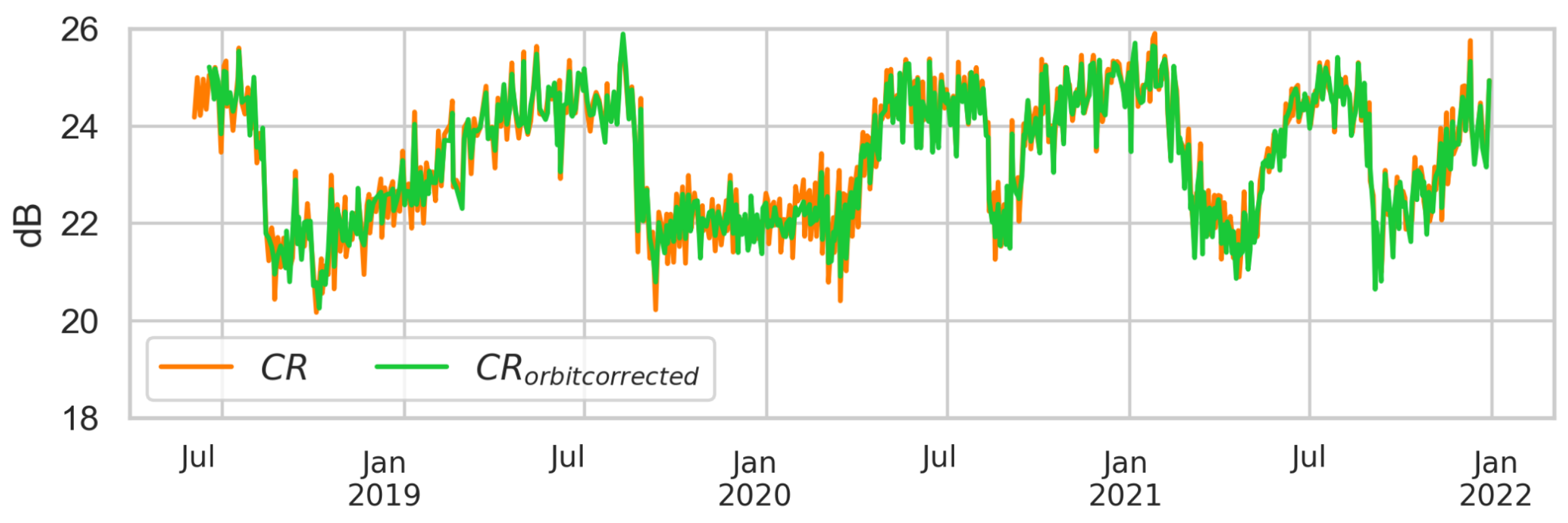
Figure 2. CR time series C R ( t ) with and without orbit corrections.
Remotesensing 16 00835 g002
Figure 3. Time series of NDVI data and preprocessed optical signal s 2 v e g ( t ) for the data fusion. The raw NDVI product and the cloud-filtered NDVI are also represented.
Remotesensing 16 00835 g003
Figure 4. Global scaling function used to scale CR to the NDVI domain of variation. The boxes extend from 25th to 75th percentiles with a line at the median. The whiskers represent the 5th and 95th percentiles.
Remotesensing 16 00835 g004
Figure 5. Time series of scaled CR corrected for orbit effects C R s o ( t ) , weighed average s 1 v e g ( t ) , and the Radar Harvest Detection Index (RHDI).
Remotesensing 16 00835 g005
Figure 6. Location of fields used in examples in this study.
Remotesensing 16 00835 g006
Figure 7. Biomass Proxy, S 1 v e g and S 2 v e g time series over two neighboring wheat fields in France, under clear (a) and cloudy (b) sky conditions during the May–June–July period.
Remotesensing 16 00835 g007
Figure 8. Biomass Proxy maps for a 40 ha maize field in France. The ratios between NDVI and CR pixel values and field averages of the respective images, r a t i o s 1 , i ( x , y ) and r a t i o s 2 , m ( x , y ) , are also represented.
Remotesensing 16 00835 g008
Figure 9. Maps of Biomass Proxy (a), 10-day scaled CR composites (b) and 10-day NDVI composites (c) over the full season of a 40 ha maize field in France.
Remotesensing 16 00835 g009
Figure 10. Biomass Proxy, cloud-free NDVI observations, s 1 v e g and s 2 v e g time series for barley and canola (a) demonstrating different features associated with color changes, particularly evident for barley during senescence (b) and for canola during flowering (c).
Remotesensing 16 00835 g010
Figure 11. Biomass Proxy, cloud-free NDVI observations, s 1 v e g and s 2 v e g time series for onion and yellow mustard (a) in an 8 ha field in Flevoland, demonstrating that radar and optical data are sensitive to different biophysical properties. Onions (b), with higher water content, are associated with high Biomass Proxy values (picture taken 28 August 2020), while yellow mustard (c), with its denser canopy, is associated with higher NDVI values.
Remotesensing 16 00835 g011
Figure 12. Biomass Proxy, cloud-free NDVI observations, S 1 v e g and S 2 v e g time series for a good-performing (a) and a bad-performing (b) sugarcane field, illustrating the complementary use of these signals in field performance assessment. In addition, high- and low-performance field seasons are given and represented by the green and red lines for Biomass Proxy (c) and NDVI (d), respectively, reflecting yields above the 75th percentile and below the 25th percentile. For illustrative purposes, a typical sugarcane field (e) is also given.
Remotesensing 16 00835 g012
Figure 13. Biomass Proxy time series for 1000 fields of maize (a) and 1000 fields of wheat (b) spread over three regions, demonstrating the scalability of the algorithm and the consistency of the results. The thick lines represent the average of the time series of the region.
Remotesensing 16 00835 g013
Disclaimer/Publisher’s Note: The statements, opinions and data contained in all publications are solely those of the individual author(s) and contributor(s) and not of MDPI and/or the editor(s). MDPI and/or the editor(s) disclaim responsibility for any injury to people or property resulting from any ideas, methods, instructions or products referred to in the content.