Sound Speed Inversion Based on Multi-Source Ocean Remote Sensing Observations and Machine Learning

Abstract

Ocean sound speed is important for underwater acoustic applications, such as communications, navigation and localization, where the assumption of uniformly distributed sound speed profiles (SSPs) is generally used and greatly degrades the performance of underwater acoustic systems. The acquisition of SSPs is necessary for the corrections of the sound ray propagation paths. However, the inversion of SSPs is challenging due to the intricate relations of interrelated physical ocean elements and suffers from the high costs of calculations and hardware deployments. This paper proposes a novel sound speed inversion method based on multi-source ocean remote sensing observations and machine learning, which adapts to large-scale sea regions. Firstly, the datasets of SSPs are generated utilizing the Argo thermohaline profiles and the empirical formulas of the sound speed. Then, the SSPs are analyzed utilizing the empirical orthogonal functions (EOFs) to reduce the dimensions of the feature space as well as the computational load. Considering the nonlinear regression relations of SSPs and the observed datasets, a general framework for sound speed inversion is formulated, which combines the designed machine learning models with the reduced-dimensional feature representations, multi-source ocean remote sensing observations and water temperature data. After being well trained, the proposed machine learning models realize the accurate inversion of the targeted ocean region by inputting the real-time ocean environmental data. The experiments verify the advantages of the proposed method in terms of the accuracy and effectiveness compared with conventional methods.

1. Introduction

Sound signals are an important medium for mild-long-range underwater signal propagation. Sound speed is a key quantity for underwater communications, underwater navigation and localizations [1,2]. Due to the inhomogeneous water body, the paths of sound rays are bent and the estimated sound speed varies depending on the interrelated and temporal–spatial-varying water parameters, such as the temperature, salinity and depth. To incorporate the sound speed into the system, the assumptions of fixed sound speed (about 1500 m/s) or measured sound speed profiles (SSPs) are generally considered in underwater acoustic applications. An erroneous sound speed directly causes the measured sound rays to deviate, which greatly degrades the performance of the underwater acoustic system. To measure SSPs requires deploying complicated sensors at a high cost. Furthermore, the temporal–spatial variations in underwater conditions easily make the measured SSP outdated. To avoid these errors from mismatches between the measured sound speed with the real one, the inversion of SSPs has attracted the researchers’ attention and become one necessary approach to improve the performance of underwater signal processing [3,4,5].

The inversion of the sound speed field utilizing measurements is intuitive, which requires deploying instruments such as the sound velocity profilers or thermohaline profilers to obtain direct sound speed quantities or indirect sound speed-related parameters [6]. These methods cannot cover large-range ocean regions, and their performance is limited due to being time-consuming and the high cost. From this background information, the indirect inversion methods of sound speed are developed. The earliest technique for the indirect inversion of the sound speed is ocean acoustic tomography (OAT), which was firstly proposed by Munk [7] and used to monitor the ocean mesoscale fluctuations through the measured sound propagation time. Although OAT-based technology can obtain more accurate results than measurement methods, the OAT-based inversion is the optimization with the designed cost function and requires a large amount of calculations of sound speed models. The aforementioned inversion methods are difficult to apply on the current underwater acoustic systems with the requirements of fast speed and low cost.

The relations of various physical ocean parameters, such as water temperature and water salinity, have continued to be explored, and the research on the ocean temperature and salinity fields promotes the development of SSP inversions. Many works have proved the correlations among various SSP-related parameters [8,9], so it is meaningful to explore the nonlinear mapping relations between sound speed and other ocean parameters. The artificial intelligence (AI) technologies such as machine learning (ML) are powerful solvers to mine the inner relations of marine data and explore the unknown mapping relations. Jain et al. [10] proposed an estimation method of the sound speed from surface observations using an artificial neural network method, which considered the surface heat flux, net radiation, sea surface wind stress, dynamic height (DH) and vertical profiles of the temperature and salinity and utilized the multilayer perceptron (MLP) model with two hidden layers. The paper [11] proposed a convolutional long short-term memory (LSTM) network for SSP inversion, which considered the Argo-based SSPs. Due to the rapid accumulation of marine data, a large number of highly valuable ocean observation data provide sufficient training datasets. For the real-time data processing, it is necessary to characterize and represent the available ocean sound speed data. Considering the temporal–spatial correlations, the reduced-dimensional representations realize the parameterized descriptions of the sound speed field with a few basis functions. The empirical orthogonal function (EOF)-based construction method for the sound speed field greatly reduces the number of required parameters [12]. The papers [13,14] proposed single empirical orthogonal function regression (sEOF-r)-based construction methods for the ocean sound speed field. A multilayer perceptron neural network was proposed to learn the SSPs’ functional transformation and output the desired EOF coefficients for inversion [15]. In 2017, Bianco induced the dictionary learning into the representation of the sound speed field, which greatly improved the construction accuracy with sparse features [16]. Yan utilized dictionary learning for the sparse encoding and compressing storage of SSPs [17]. The paper [4] proposed a learned dictionary-based supervised framework for SSP classifications. The paper [5] proposed an interpretable deep-K singular-value decomposition model to analyze the SSP data with uncertainties.

Due to the development of an integrated air–sea network, satellite remote sensing provides more available data for the rapid acquisition of the sound speed in the large-scale ocean area. Depending on the satellite, remote sensing observations have potential for the achievement of near-real-time and accurate SSP inversion. Based on the Argo data and the sea surface datasets, the paper [18] considered the eddy kinetic energy in the sEOF-r inversion framework, which proved the concept of global SSP inversion. The paper [19] incorporated XGBoost into the field of sound speed inversion, which further improved the estimation accuracy of SSPs by utilizing satellite remote sensing data. As with the aforementioned investigations, ML-based SSP inversion methods are developing and achieve good results in many aspects, such as feature representations, ML model establishment and SSP-related datasets generation. However, the exploration of available data has developed immaturely, where the sea surface remote sensing data are limited for SSP inversion with different depths. There is a lack of a general framework for the SSP inversion by considering the remote sensing data and other ocean observation data. There is also lack of the physical interpretation of the relations between the sea surface parameters and the sound speed field disturbances.

To fill this gap and aim to the accurate, fast, low-cost sound speed inversion over large-scale sea regions, this paper proposes an inversion method for the ocean sound speed field based on multi-source ocean remote sensing observations and the designed ML models. The major contributions of this paper are as follows.

(1)

Multi-source remote sensing datasets are utilized, which include the global ocean Argo datasets to generate SSPs and ocean sea surface remote sensing datasets to provide information, such as sea level anomalies (SLA) and the sea surface temperature (SST), shallow-water temperature data and localization information. The utilization of multi-source remote sensing datasets explores the feasibility of SSP inversion over a large-scale ocean area, and the utilization of water temperature observations in different depths further improves the accuracy of SSP inversion in the local sea region.

(2)

The EOF-based characterization is exploited to reduce the dimensions of Argo-based SSPs. The sound speed reconstruction performances with different-order EOFs are compared and analyzed. Combining with the dynamic ocean phenomena, the EOF and PC parameters are analyzed to explore their physical meaning. Then, the first five orders of coefficients are chosen as model labels to achieve the tradeoff of inversion accuracy and computational load.

(3)

Combining the reduced-dimensional characterization of the sound speed field and multi-source remote sensing datasets, this paper provides a novel and general framework for SSP inversion, where a single ML model or combined ML models are exploited considering different inversion performances for each order of EOF. Experiments are executed to verify the advantages of the proposed method in term of the accuracy and robustness for SSP inversion, especially for shallow-water cases, due to the consideration of the temperature at different water depths.

2. Materials and Method

In this section, we introduce the involved datasets, the EOF representations of the SSP datasets and the ML models. On the basis of the datasets analysis and typical models for the nonlinear estimation for ocean parameters, a general SSP inversion method is proposed.

2.1. Datasets

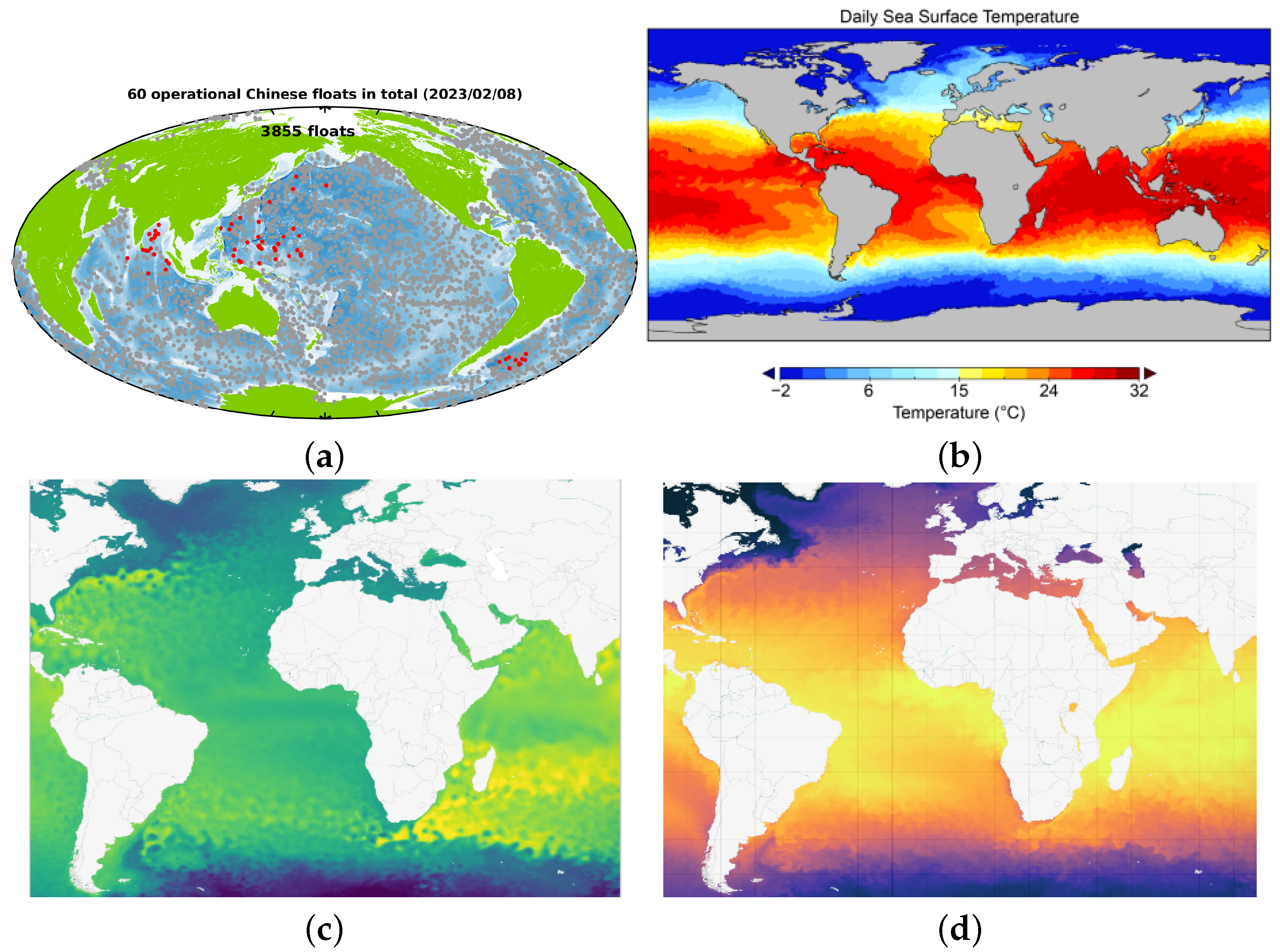
The datasets involved in this paper are the Global Argo Ocean Observation dataset and the satellite remote sensing-based National Oceanic and Atmospheric Administration (NOAA) and Copernicus Marine Environment Monitoring Service (CMEMS) datasets, which are shown in Figure 1. Argo is a global ocean project initiated by scientists from the United States, Japan and other countries in the late 1990s [20]. In Figure 1, the first subfigure shows the distribution of active buoys in the Argo observation network as of 8 February 2023. The red circle dots represent Chinese Argo program buoys. This paper uses the Argo Grid Dataset provided by the Argo Live Data Center (http://www.argo.org.cn/ (accessed on 8 February 2023)). The NOAA dataset is provided by the National Oceanic and Atmospheric Administration and is designed to address the risk of climate disasters. The SST data are from NOAA’s 1/4° Optimum Daily SST (OISST) database, primarily from the observations of the Advanced Very High Resolution Radiometer (AVHRR) satellite, which has covered a large-scale temperature field since 1981. Copernicus is the European Union’s Earth observation project, which uses observational data from space satellites and in situ measurements for the purpose of making free, open, near-real-time ocean datasets available worldwide. The data in Figure 1c,d include the data of the SLA and SST, which are obtained from the Copernicus C3S (Copernicus Climate Change Service) series of database products.

2.2. EOF Analysis of SSP

The key to the utilization of satellite remote sensing data is to build the regression relationship between the ocean sound speed field and remote sensing parameters. Benefiting from the advantages of an EOF analysis in data compression, SSPs are parameterized with reduced dimensions. An EOF analysis generates the Principal Components (PCs) parameter, which reflects the change weight of EOFs in the time dimension. Then, the regression relationship between the SSP and remote sensing parameters is transformed into the regression relation between multi-order PCs and remote sensing parameters. When it comes to analyzing the EOFs of the SSPs, we can obtain the multi-order EOFs and PCs. Then, we use the remote sensing dataset to fit the relation between the first k orders of PCs and sea surface parameters according to

$$\begin{array}{c}\hfill {\alpha }_k={\alpha }_{0k}+{\alpha }_{1k}SST+{\alpha }_{2k}SLA+{\alpha }_{3k}SST\times SLA\end{array}$$

(1)

where ${\alpha }_k$ is the corresponding PC for the kth-order EOFs. ${\alpha }_{0k}$, ${\alpha }_{1k}$, ${\alpha }_{2k}$ and ${\alpha }_{3k}$ are the regression coefficients, which can be obtained using the least squares method. With Equation (1), the regression coefficients are achieved. When we input real-time remote sensing surface parameters, the PCs can be calculated. Combined with the known EOFs, the SSPs are recovered.

2.3. Machine Learning Models

The machine learning models in this paper include multiple linear regression (MLR), support vector regression (SVM), MLP and XGBoost. These four models are widely applied to the parameter estimation of ocean environments. We give a brief introduction for these models.

MLR analyzes the approximate linear relationship between a single independent variable and multiple dependent variables based on statistical theory [25]. Given a group of observations $\left\{Y,x_1,x_2,\cdots ,x_k\right\}$, Y is the fitting value, ${\left\{x_i\right\}}_{i=1}^k$ are independent explanatory variables, and then the model of MLR is given by

$$\begin{array}{c}\hfill Y={\beta }_0+{\beta }_1{x}_1+{\beta }_2{x}_2+\cdots +{\beta }_k{x}_k+\epsilon \end{array}$$

(2)

where ${\beta }_i$, $i=1,2,\cdots ,k$ is the regression coefficient, ${\beta }_0$ is the constant term and $\epsilon$ is the error term.

SVR is a branch of SVM for a regression problem [26]. The training process of SVR is transformed as an optimization problem (3) given datasets $\left\{\left(x_1,y_1\right),\left(x_2,y_2\right),\cdots ,\left(x_n,y_n\right)\right\}$,

$$\begin{array}{c}\hfill \begin{array}{c}min\frac{1}{2}{∥w∥}^2+C{\displaystyle \sum _{i=1}^n}\left({\xi }_i^{on}+{\xi }_i^{down}\right)\\ s.t.\left\{\begin{array}{c}{y}_i-〈w,\Phi \left(x\right)〉-b\le \epsilon +{\xi }_i^{on}\\ -y_i+〈w,\Phi \left(x\right)〉+b\le \epsilon +{\xi }_i^{down}\\ {\xi }_i^{on},{\xi }_i^{down}\ge 0\left(i=1,2,\cdots ,n\right)\end{array}\right.\end{array}\end{array}$$

(3)

where $\Phi \left(x\right)$ is the nonlinear mapping function, w is the weight vector, b is the compensation term and $\epsilon$ is the tolerance deviation of the interval band. C is the error penalty factor, which controls the tradeoff between the estimated function and the tolerant deviation amount of $\epsilon$. ${\xi }_i^{on}$ and ${\xi }_i^{down}$ are introduced as the slack variables to cope with the otherwise infeasible constraints of the convex optimization problem.

XGBoost is an addition model that integrates multiple lift trees [27]. Assume there are K decision trees, the tree model for the tth iteration training is $f_t\left(x\right)$, and the predicted value ${\widehat{y}}_i^{\left(t\right)}$ is given by

$$\begin{array}{c}\hfill {\widehat{y}}_i^{\left(t\right)}=\sum _{k=1}^t{f}_k\left(x_i\right)={\widehat{y}}_i^{\left(t-1\right)}+f_t\left(x_i\right)\end{array}$$

(4)

where $x_i$ is the ith sample input. The objective function is given by

$$\begin{array}{c}\hfill Obj\left(f_t\right)=\sum _{i=1}^{n}L\left(y_i,{\widehat{y}}_i^{\left(t\right)}\right)+\Omega \left(f_t\right)\end{array}$$

(5)

where the loss function is $L=\frac{1}{2}{\left(y_i-{\widehat{y}}_i\right)}^2$ and the regulation term is $\Omega \left(f_t\right)=\gamma T+\frac{1}{2}\lambda {\displaystyle \sum _{j=1}^T}{w}_j^2$. n is the sample number, $\gamma$ and $\lambda$ are the regulation coefficients and T is the number of samples of multi-leaf nodes in the decision tree.

MLP is a fully connected feedforward neural network, which is composed of the input layer, hidden layer and output layer [28]. The MLP model is given by

$$\begin{array}{c}\hfill y=f\left(\sum _{i=1}^n{w}_i{x}_i\right),i=1,2,\cdots ,n\end{array}$$

(6)

where y is the output of the network, f is the activation function, $x_i$ and $w_i$ are the input of the ith neuron and weight and n is the number of neurons.

2.4. Proposed Inversion Method of SSPs

This subsection proposes an inversion method of the sound speed based on multi-source ocean remote sensing observations, which combines the datasets and machine learning models with the reduced-dimensional characterization of the SSP.

The inversion results use remote sensing data depending on the correlation between the parameters of sea surface and the sound speed field. In the interior of the ocean, ocean dynamic activities lead to different disturbances in the sound speed field. Random disturbance information is not fully covered in sea surface parameters, so the inversion performance will be worse. It is limited for the sound speed of the whole sea depth only using remote sensing data of the sea surface. It is necessary to reasonably expand datasets of the sound speed field. Therefore, we add a very small amount of shallow-water temperature data to reduce the estimation error of the sound speed in shallow sea; on the other hand, according to the characteristics of the spatial variation in the ocean sound speed, this paper adds the longitude and latitude of the marked sea area as the position information to optimize the SSP inversion results.

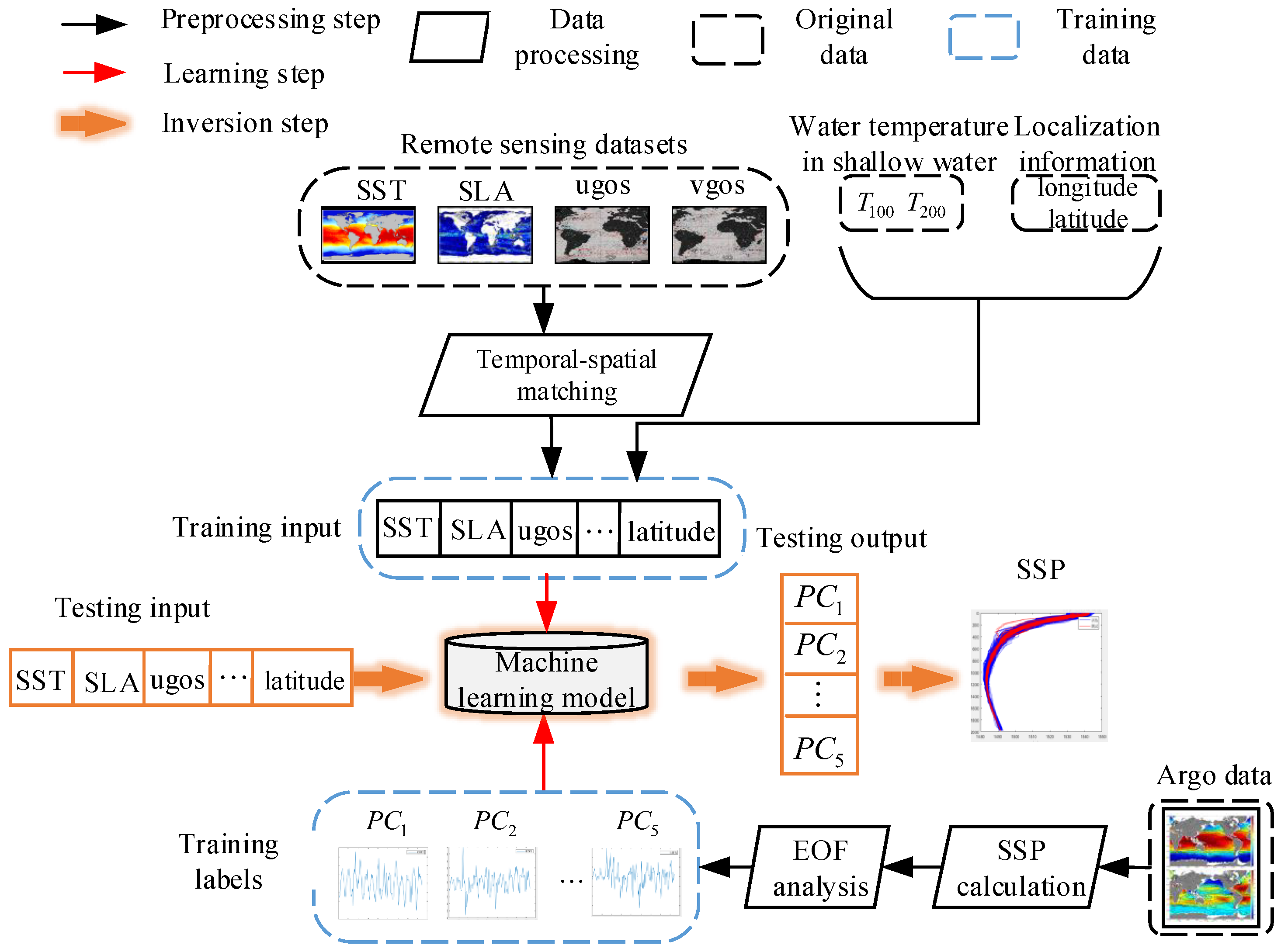
The framework of the inversion method is shown in Figure 2. The whole diagram includes three steps: preprocessing of the grid data, training of the machine learning model and the real-time inversion of the SSP.

• Data preprocessing: In the part of data preprocessing, different types of remote sensing data are required to be space-time matched. Through converting the daily average data to the monthly average data, we can keep the datasets consistent in time resolution. For the spatial resolution, two-dimensional interpolation is used to arrive at the consistency of the latitude and longitude.
• Model training: We combine the Argo thermohaline profiles and empirical formulas for the sound speed to generate a large number of SSP samples as training datasets. Through an EOF analysis for these SSP samples, the PCs are treated as the training labels for the model training. In the training part of machine learning, eight kinds of ocean environmental parameters are concatenated as input vectors, i.e., the SST, SLA, water velocity of the sea surface turning to the east (ugos), water velocity of the sea surface turning to the north (vgo), water temperature of 100 m and 200 m beneath the surface in shallow water ($T_{100}$ and $T_{200}$) and the longitude and latitude of the target sea regions. The above parameters and labels are input into different machine learning models to train, and then the inversion model of the SSP is established by tuning the optimal hyperparameters.
• SSP inversion: After the off-line training, the model is on-line deployed. Only a small number of sea surface data and temperature data are required for the SSP inversions, which has the advantages of fast estimation, low-cost deployment and large-scale applications.

3. Numerical Simulation

This section uses measured data to verify the superiority of the proposed method in SSP inversion. The experimental results present the processed datasets, the time-varying characteristics of the sound speed field based on PCs and the SSP inversion results.

3.1. Experimental Datasets

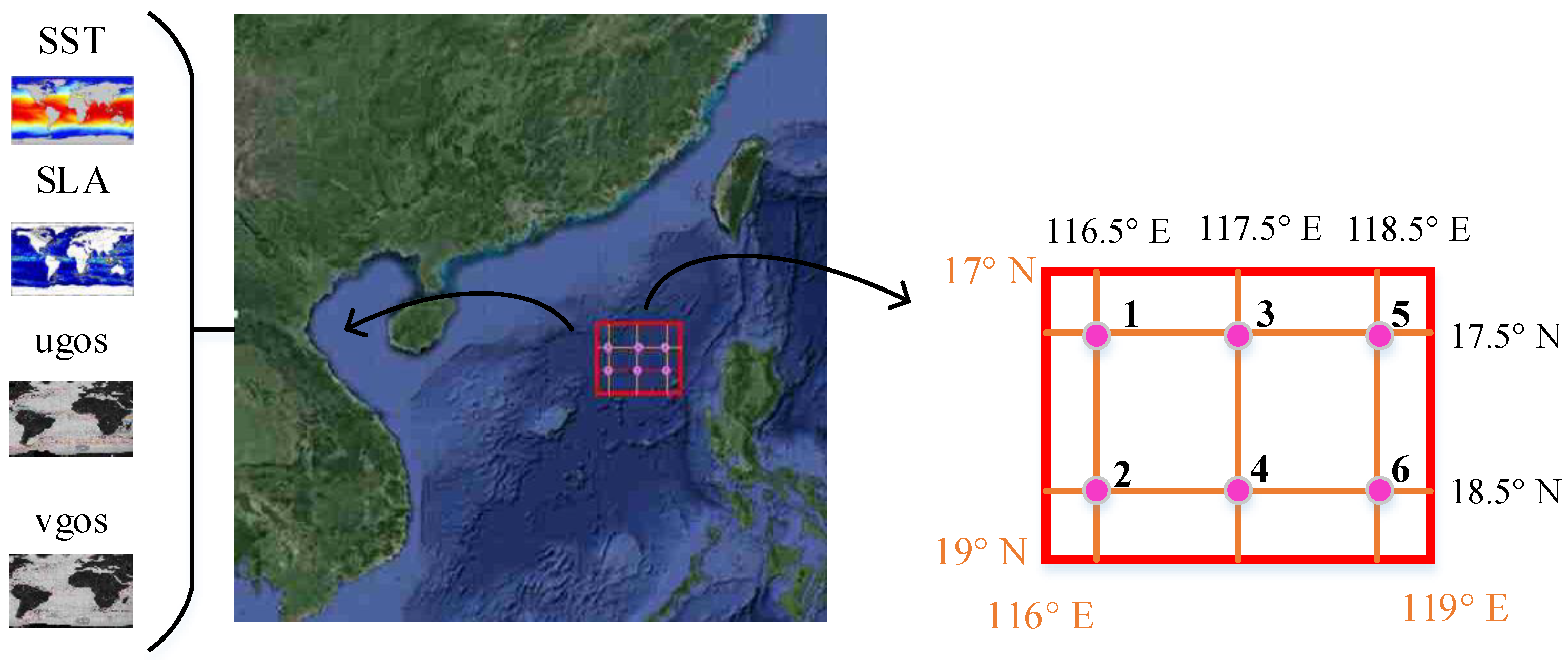
The target ocean region is the central region of the China south sea with the longitude range 116°E∼119°E and latitude range 17°N∼19°N. The sea region is subject to a monsoon climate and the influence of the Kuroshio invasion, and the activities such as the mesoscale vortex, front and turbulence are frequent. It causes random fluctuations in the temperature and salty field in the ocean, and the uncertainty of various environmental factors intensifies the difficulties for the inversion of the sound speed field.

The spatial resolution of the Argo datasets adopted in this paper is $1^{°}\times 1^{°}$. The six grid points of Argo are considered as shown in Figure 3. The monthly average Argo thermohaline profiles from 2004 to 2016 are taken as the original data. We utilize the Leroy empirical formula to generate SSP datasets, in which 936 SSP samples are taken as the training datasets and 72 SSP samples in 2017 are treated as the testing datasets. The reason for choosing Leroy’s empirical formula is that the sea water temperature in the South China Sea in the summer may exceed $30$ °C, while Leroy’s empirical formula is applicable to the sea water temperature range of −2∼34 °C. This paper uses sea surface remote sensing parameters including the SST, SLA and SSV, which are listed in

Table 1. Parameters of datasets.

Parameters	Datasets	Time Resolution	Space Resolution
Thermohaline	Argo	Monthly average	$1^{\circ }\times 1^{\circ }$
SST	NOAA	Daily average	$0.{25}^{\circ }\times 0.{25}^{\circ }$
SLA and SSV	CMEMS	Daily average	$0.{25}^{\circ }\times 0.{25}^{\circ }$

.

3.1.1. Data Matching and Correlation Analysis

According to Table 1, the temporal–spatial resolution of the remote sensing data is higher than the Argo data, so then it is necessary to perform spatial–temporal matching to ensure a consistent resolution across the different datasets. To unify the time resolutions, we take the monthly average of the daily averages in the sea surface remote sensing data, and finally, all the kinds of the remote sensing parameters have 1008 monthly average data samples. The unification of the spatial resolutions requires a two-dimensional interpolation as shown in Figure 4, which is operated using the interpolation function.

3.1.2. Correlation Analysis

The correlation between the sea surface remote sensing parameters and shallow-water temperature is analyzed as a prerequisite for the accurate inversion of the sound speed. The Spearman correlation coefficient measures the degree of dependence between variables based on monotonicity, which is in the range $\left[-1,1\right]$. When the coefficient is positive, it indicates a positive correlation. The more closer to 1 of the absolute value, the stronger the correlation is. The Spearman coefficient ${\rho }_s$ is given by

$${\rho }_s=1-\frac{6{\displaystyle \sum _{i=1}^N}{d}^2}{N^3-N}$$

(7)

where $d=r_x-r_y$, and $r_x$ and $r_y$ are the rank of X and Y. N is the sample number.

Figure 5 shows the Spearman coefficients between the SLA, SST and water temperature with water depths of 50 m, 100 m, 150 m, 200 m and 300 m. As shown in Figure 5, the SST and SLA are correlated with water temperatures of different depths. The correlation coefficient reaches above 0.6, which verifies the feasibility of using remote sensing parameters of the sea surface to invert the sound speed field.

3.2. Analysis of SSP Datasets

Figure 6 shows 168 monthly average SSP samples corresponding to grid point 1 from 2004 to 2017. The blue part represents 156 SSPs in the training set, and the red part represents 12 SSPs in the testing set.

After the data processing, we analyze the EOF coefficients of the datasets to decide the model output labels. We define the cumulative variance contribution rate (CR) of the first k orders of EOFs as

$$CR=\frac{{\displaystyle \sum _{i=1}^k}{\lambda }_i}{{\displaystyle \sum _{j=1}^M}{\lambda }_j}$$

(8)

where ${\lambda }_i$ is the eigenvalue of the ith-order EOF.

Figure 7 and

Table 2. Performance of reconstructed SSP with different EOF orders.

EOF Order	VAR CR	Cumulative VAR CR	Error (m/s)
1	67.91%	67.91%	1.13
2	17.21%	85.12%	0.77
3	7.49%	92.61%	0.54
4	3.19%	95.80%	0.41
5	1.45%	97.25%	0.33
6	0.82%	98.07%	0.28

present the reconstruction performance of the sound speed field with different-order EOFs. In Figure 7a, the variance CR decreases as the order of the EOF increases. The first-order EOF contributes the most variance CR, which arrives at $67.91\%$. The sixth-order EOF contributes less than $1\%$. The result shows that the main features of the sound speed field exist in the first five orders of EOFs. Figure 7b reflects the construction errors at different depths with different EOF orders. On the whole, the reconstruction error decreases as the depth increases. When the depth is greater than 1200 m, the sound speed error is less than 0.2 m/s and tends to be flat. When the depth is less than 100 m, the error of the sound speed increases significantly and the motion is obvious, especially in the vicinity of 50 m, and the reconstruction error using the first three orders of EOFs is greater than 1 m/s. With the order increasing, the error of the sound speed at each depth decreases, especially the reconstruction accuracy of the sound speed field within 1000 m, which is significantly improved. In Table 2, the construction error is 0.33 m/s when choosing the first five orders of EOFs, and the first five orders of the EOFs are enough to reconstruct the acoustic speed field as the prior information considers the tradeoff between the accuracy and the computational load. The first five orders of the EOFs and PCs can be estimated to reconstruct the sound speed field in the target sea area.

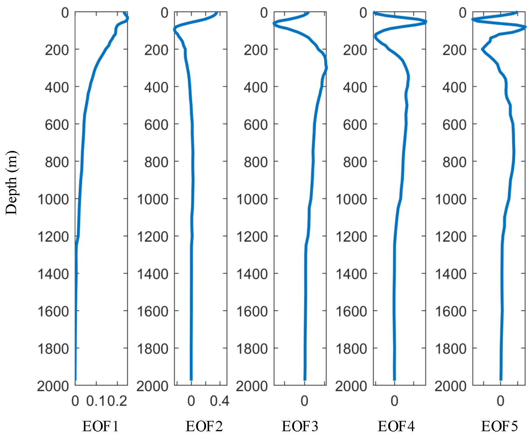
Figure 8 shows the first five orders of EOFs for the reconstruction of the sound speed field. In the figure, the jitters of the EOF are concentrated in water layers with less than 500 m depth. When the depth is greater than 1000 m, the amplitude of each order of EOF tends to 0. The phenomenon proves that the disturbance of the upper ocean speed field is relatively active. The EOF reflects the characteristics of the spatial distribution for the sound speed.

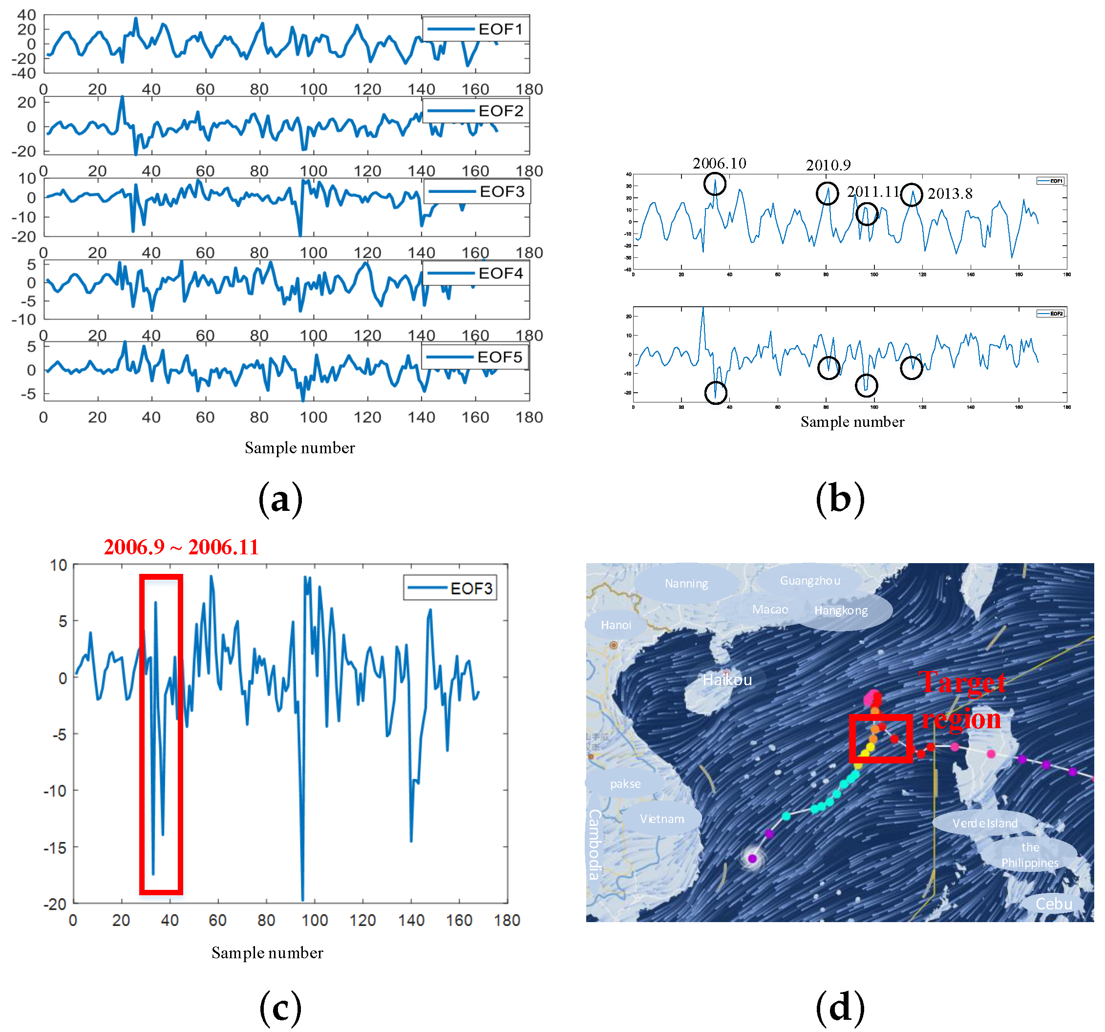
Figure 9 shows the first five orders of PCs corresponding to the first five orders of EOFs. In Figure 9a, the fluctuation range of the first order is obviously larger than the last four orders, and the fluctuation trend is relatively regular. The amplitude gradually increases from May to August every year and decreases from January to February in the next year. The maximum value is mostly concentrated in August and September, and the minimum value mainly appears in February and March. The above change law corresponds to the annual cycle characteristics of the sound speed field changing with the seasons. From this analysis, it can be seen that the first-order PC essentially reflects the annual cycle change rule of the sound speed field, and the sea water temperature at this time is the dominant factor for sound speed variation.

The amplitude variation law of the second-order PC is similar to that of the first-order PC, which also has annual cycle characteristics. However, there are outliers at some points as shown in Figure 9b, which are noted by circle. It can be seen that outliers appear at the time points concentrated in the summer and autumn seasons, and the corresponding amplitude changes are exactly opposite to the first-order PC. Because the second order of the ocean vertical profile is usually associated with the thermocline [29], the outliers of the second-order PC may be related to the abrupt changes in the salinity in the upper ocean layer.

Different from the change law of the first two orders of PCs, the last three orders of PCs jitter more frequently and there is no obvious annual cycle characteristics, whose amplitude range is reduced relative to the first two orders of PCs. It is because higher-order PCs tend to contain subtle disturbance information of sound speed fields and are particularly sensitive to the heat exchange in the ocean [30]. Figure 9c shows three consecutive outliers in the third-order PC, which correspond to the time of September 2006 to December 2006. According to the “Typhoon query” service of the China Meteorological Administration, Typhoon 619 Cimaron passed the sea area near grid point 1 (17°N∼17.7°N, 116.3°E∼116.8°E) from 31 October to 3 November 2006 as shown in Figure 9d. Its maximum wind reached 10 levels. From this analysis, it can be seen that the outliers of the third-order PC are most likely related to severe weather, such as typhoons, which causes intense mixing of the upper ocean and dramatic changes in the water temperature and salinity, resulting in disturbances of the ocean sound speed field.

Through analyzing the physical meanings of the first five orders of PCs, it can be seen that the first two orders of PCs reflect the seasonal variation in the speed field. Some of the outliers of the second PC may be associated with the upper ocean salinity field. The last three orders of PCs mainly reflect the subtle disturbance phenomena of the ocean sound speed field from dynamic activities such as the front and turbulence, which increases the difficulty of retrieving the sound speed field.

Figure 9. The first 5 orders of PCs and analysis. (a) the first 5 orders of PCs; (b) the 2nd–order PC; (c) the 3rd–order PC; and (d) the track of Typhoon Cimaron [31].

Figure 9. The first 5 orders of PCs and analysis. (a) the first 5 orders of PCs; (b) the 2nd–order PC; (c) the 3rd–order PC; and (d) the track of Typhoon Cimaron [31].

3.3. Result Analysis of SSP Inversion

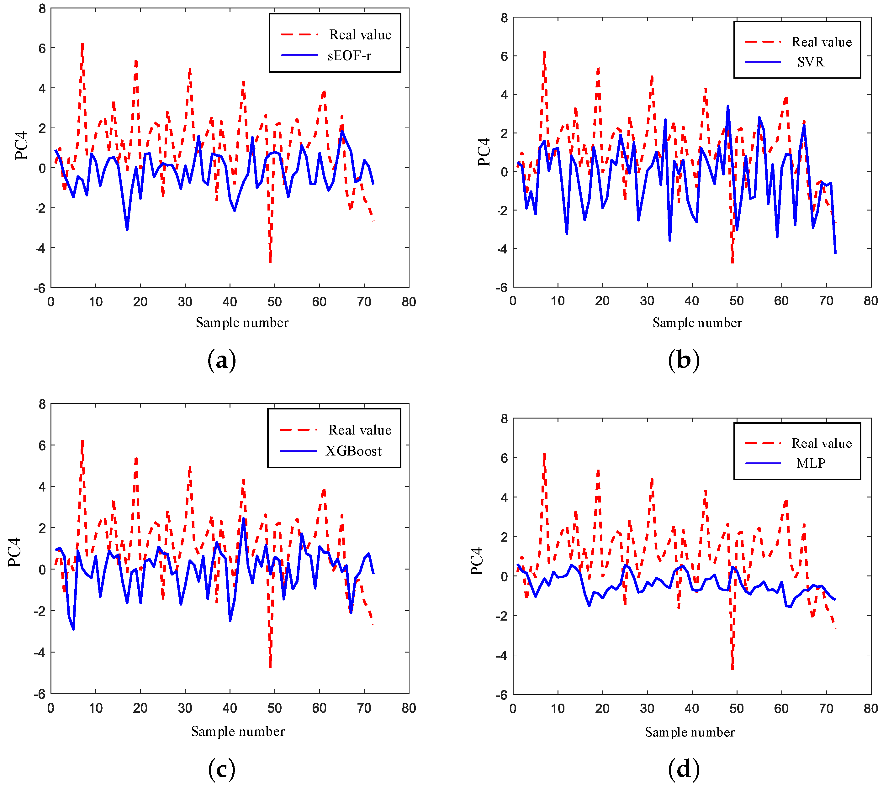
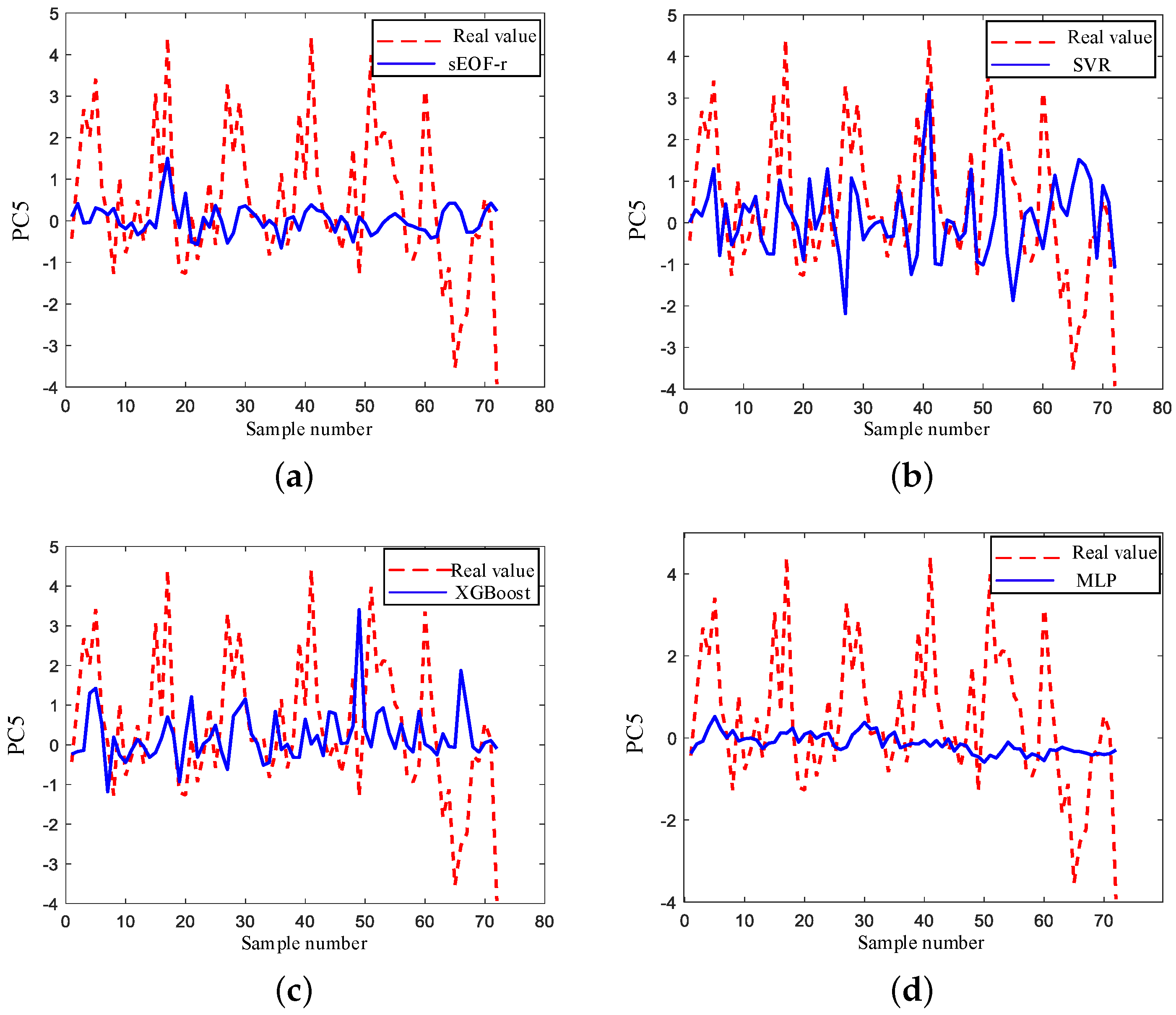
The ML models include SVR, MLP, MLR and XGboost. The SVR model uses the Gaussian kernel function. $\gamma =1$ and the penalty factor is 10. XGBoost leverages 20 categorical regression trees for learning, the learning rate is 0.1, the maximum depth of the tree is 6 and the minimum leaf node weight is set to 1. MLP uses two hidden layers, and each layer has 50 neurons. The activation function is selected as the LeakyRelu function, and the stochastic gradient descent algorithm is adopted. The initial learning rate is set to 0.015 and the loss function is the mean square error. The accuracy of the SSP inversion depends on the PCs. 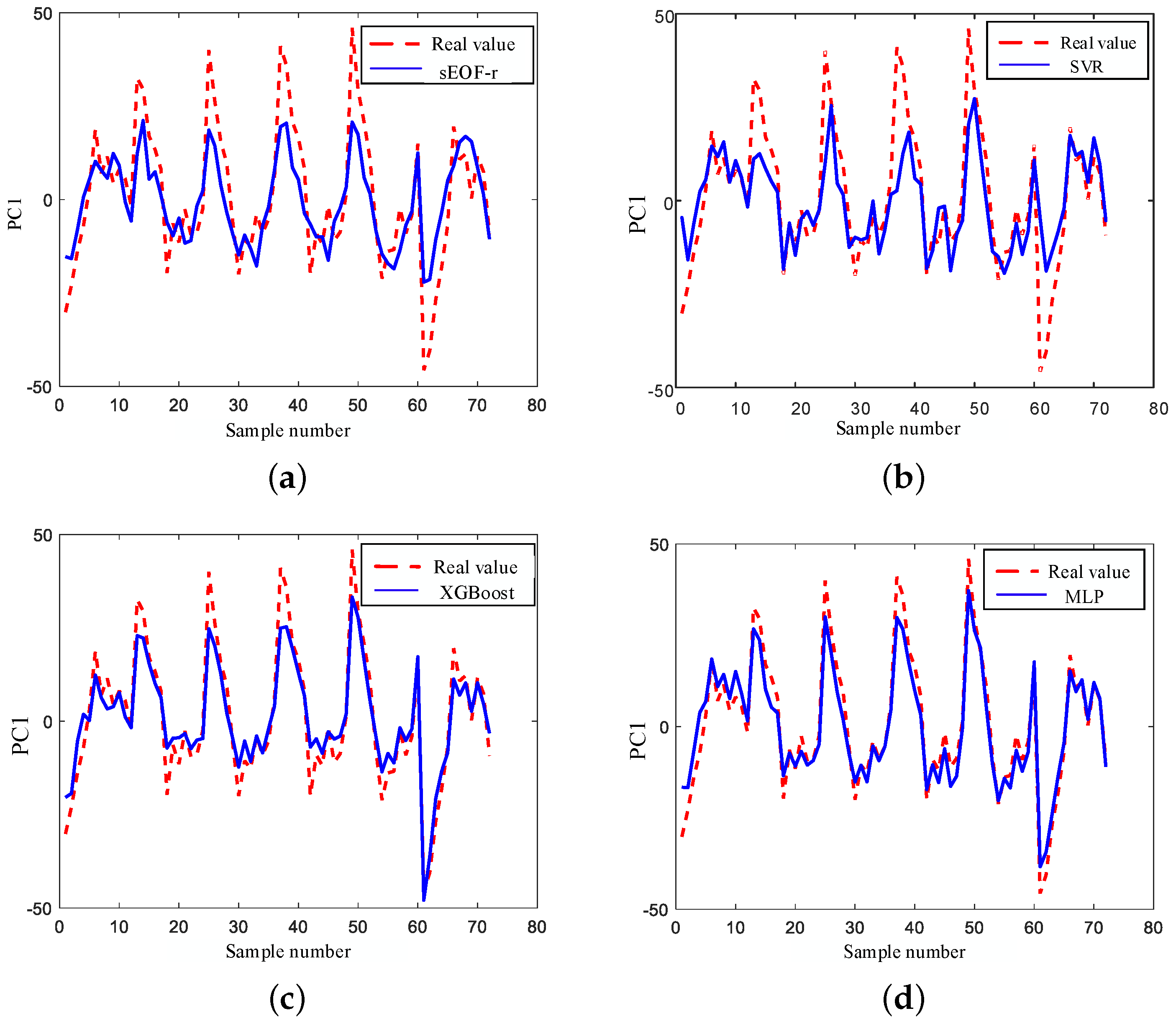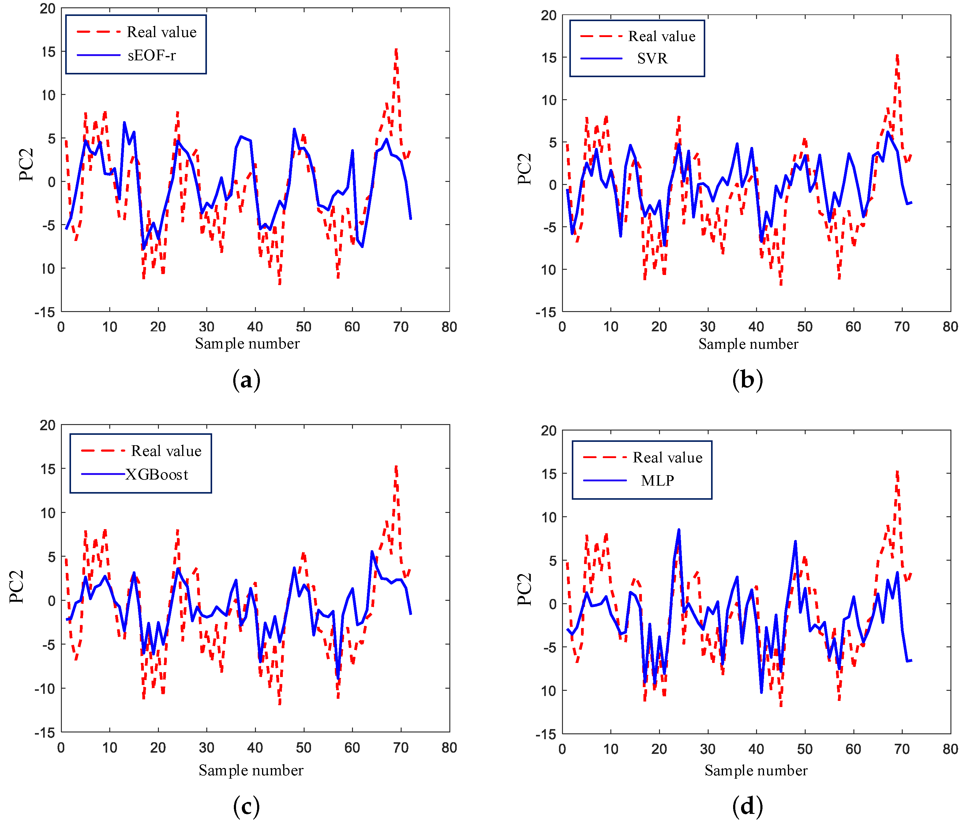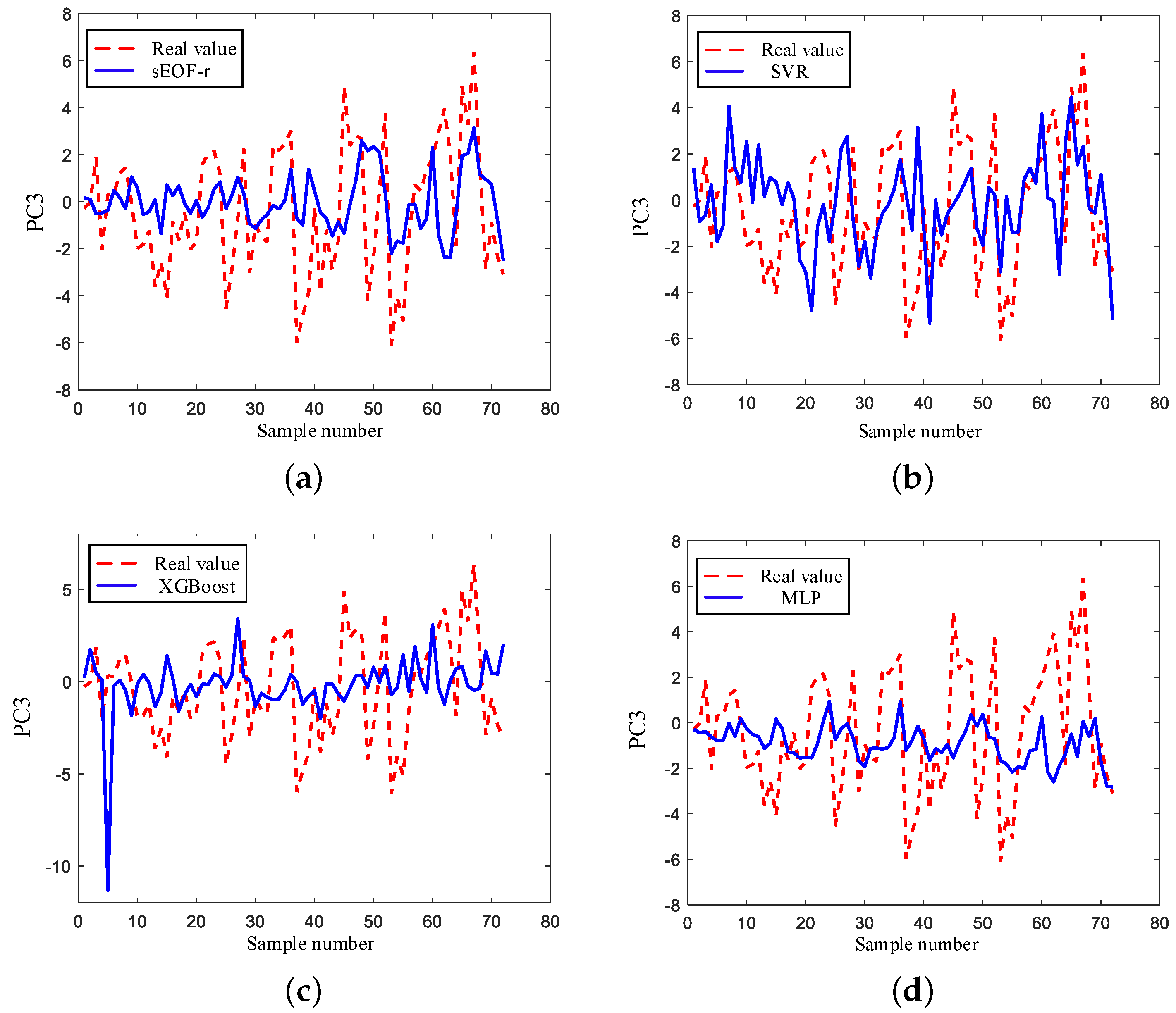From Figure 10, Figure 11, Figure 12, Figure 13 and Figure 14, the recovery performance of the dominant first five orders of PCs are compared with different ML models.

Figure 10 shows the estimation results of the first-order PC. It can be seen that all four models can learn the changes in the first-order PC, among which sEOF-r has the worst estimation performance, and it is difficult to fit the peak and jitter details of the first-order PC. SVR can learn some jitters between peaks, but its fitting results are still not enough. XGBoost and MLP have better ability in learning the peak values and the fluctuation details of the first-stage PCs, where MLP has the best fitting effect. The results prove that the nonlinear ML models have better regression results than conventional linear models. Because the first-order PC has the major information for the sound speed, the accurate estimation lays good foundations for the SSR inversion.

Figure 11 shows the estimation performance of the second-order PC. It can be seen that all the methods do not fit the details of the changes. Compared with sEOF-r, the ML models can partially learn the jitter trends. MLP has relative better performance among the compared methods. Compared with the results of the first-order PC, the worse performance is because the second-order PC not only reflects the annual cycle characteristics of the sound speed field but also is affected by other marine environmental factors, such as the abrupt change in the ocean upper salinity field.

Figure 12, Figure 13 and Figure 14 show the estimation results of the last three orders of PCs. It is worth noting that the cumulative VAR CR is only 12.13%, which is far less than the first two orders of PCs, which means the effects of the last three orders of the PC estimation accuracies on the reconstruction of the sound speed are much smaller than that of the first two orders of PCs. As a whole, the estimation results of the last three orders of PCs are significantly worse than that of the first two orders of PCs, especially MLP, which has results close to 0. SVR can estimate more peak fluctuations. In Figure 12c, XGBoost produces a large amplitude outlier when estimating third-order PCs, and the stability of the estimate is poor. As in the analysis of high-order PCs, the high-order PCs often reflect the random disturbance of the sound speed field, which contains complicated and changeable information that is hard to estimate. The MLP mode is not good at learning the subtle fluctuations of a higher-order PC in the sound speed field, which has advantages in grasping the circulation law of the climate state in the sound speed field. In addition, with SVR it is difficult to estimate the annual cyclic peak of the sound speed field; however, it can estimate the partial jitter tendency of a higher-order PC for random perturbations in the sound speed field, which has a stronger ability to learn the random disturbance of the sound speed field.

Based on the performances of ML models in learning the sound speed field, this paper integrates the results of MLP and SVR. The main step to build the novel model is to use the first two orders of PCs from the MLP estimation and the last three orders of PCs from the SVR estimation to form a new set of the first five orders of PCs and reconstruct the SSPs, which is shown in Figure 15.

To measure the inversion performance, the root mean square error (RMSE) is given by

$$RMSE=\sqrt{\frac{{\displaystyle \sum _{j=1}^N}{\displaystyle \sum _{i=1}^M}{\left[c_t\left(z_i,t_j\right)-c_r\left(z_i,t_j\right)\right]}^2}{N\times M}}$$

(9)

where $c_t\left(z_i,t_j\right)$ and $c_r\left(z_i,t_j\right)$ denote the real and the reconstructed SSP at time instant $t_j$ and the depth $z_i$. N is the sample number and M is the layer number of the depth.

Table 3. RMSE comparison of SSP inversion with different models.

ML Models	MLR	MLP	MLP + SVR	XGBoost	SVR
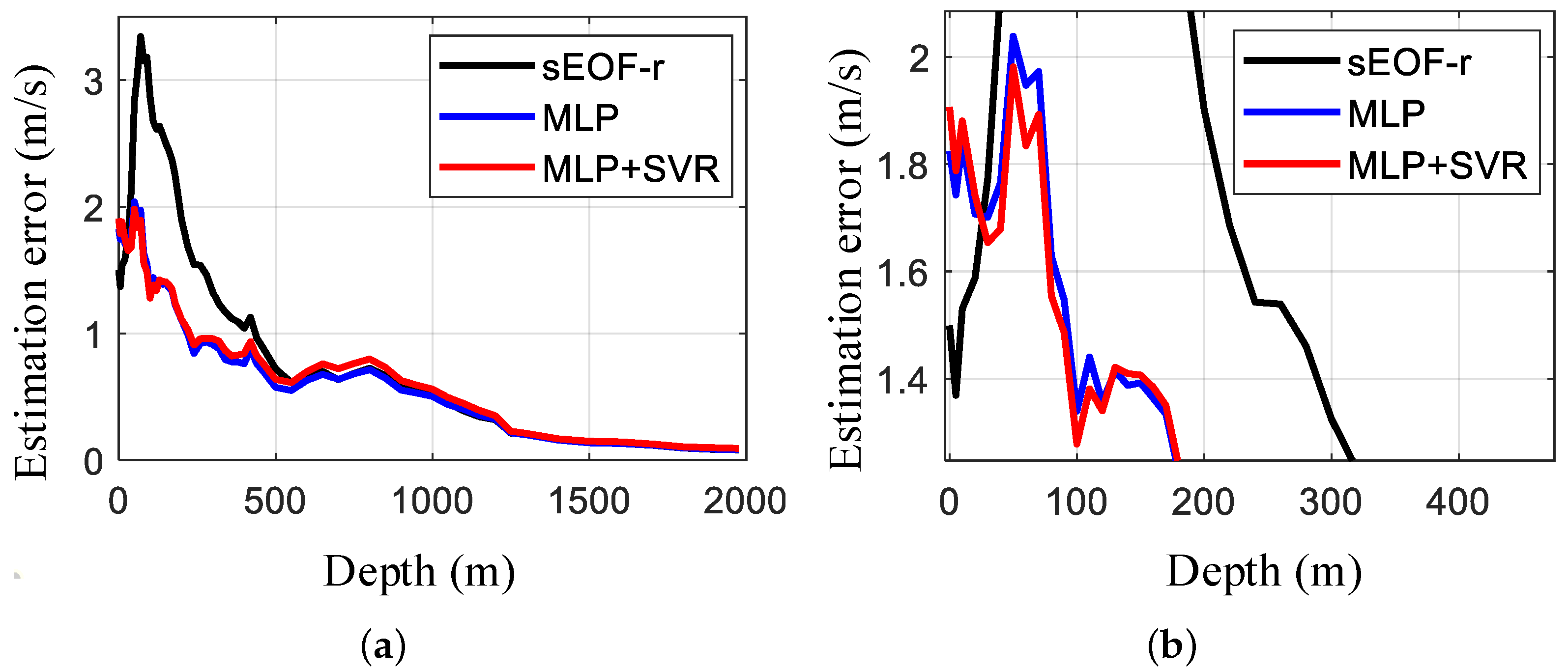
RMSE (m/s)	1.63	1.08	1.09	1.16	1.53

shows the RMSE comparisons of the different methods. It can be seen that the MLP-based inversion method has the best estimation performance. The estimation performance of the MLP combined with SVR inversion method is similar to that of the MLP inversion method.

Figure 16 compares the inversion errors between the best two proposed methods, i.e., MLP and “MLP + SVR”, and the traditional sEOF-r method at different depths. From Figure 16, it can be seen that the proposed inversion methods have smaller errors than that of the sEOF-r method at the depth of 30 m to 550 m. The estimated performance of the three methods are similar at depths greater than 550. For the combination of MLP and SVR, the inversion error is slightly smaller than that of MLP in the range of 30 m∼130 m, which decreases by about 0.116 m/s. But after 150 m, the method loses its advantage, especially the estimation errors, which are slightly higher than the traditional methods when the depth is greater than 550 m. So, we can choose MLP or the MLP and SVR combined method to retrieve SSPs when the water depth is within 550 m.

The experiments are executed on the basis of remote sensing parameters, and a very small amount of shallow sea water temperature data are added, which are from the Argo-measured thermohaline depth profile dataset. The experiments verify that the method of the ocean sound speed has significant advantages in accuracy and robustness, with the characteristics of fast, low cost and large coverage, which provides schemes for the scene requirement of sound ray correction in the underwater acoustic systems.

4. Conclusions

In this paper, an SSP inversion method based on multi-source ocean remote sensing observations is proposed. The method formulates a general sound speed field inversion framework, which is suitable for different ML models or the designed ML models. Besides the sea surface remote sensing datasets, the proposed method considers the sea surface temperature and localization information of the targeted region as the input of the ML models. Combining the convenience of the grid remote sensing dataset with the reduced-dimensional EOF-based SSPs, the feature representation and feature analysis help to realize the real-time reconstruction of the local ocean speed field. The proposed method has the advantages of simple implementation, fast estimation and accurate and good interpretability. The experiments verify that the proposed method can effectively improve the construction accuracy from 30 m to 500 m. Compared with the traditional sEOF-r method, the proposed method can estimate the sound speed with an accuracy of 1.51 m/s at the depth of 50 m∼100 m. For the whole depth SSP, the total root mean square error is reduced by about 0.55 m/s.

The proposed method explores the ML-based SSP inversion method and the inherent relations between the feature representations and physical ocean phenomenon. However, this method is still limited, which requires being further developed. (a) The datasets involved in this paper, such as the existing remote sensing parameters of the sea surface and the shallow sea water temperature data, cannot cover the perturbation information of the sound speed field, so the estimation performance of the models is limited. For dataset generation, besides the remote sensing datasets and temperature datasets, more reliable datasets are required to be explored for more accurate SSP inversion. (b) For the design of network models, DL models can provide robust and powerful learning models for SSP inversion, especially along with the number of available datasets increasing. In the future, our focus is on the design of DL-based SSP inversion models and feature representations for SSP datasets, which considers the spatial–temporal variation in the sound speed in the target ocean region.