Abstract
In response to the demand for high-precision point cloud mapping of subway trains in long tunnel degradation scenarios in major urban cities, we propose a map construction method based on LiDAR and inertial measurement sensors. This method comprises a tightly coupled frontend odometry system based on error Kalman filters and backend optimization using factor graphs. In the frontend odometry, inertial calculation results serve as predictions for the filter, and residuals between LiDAR points and local map plane point clouds are used for filter updates. The global pose graph is constructed based on inter-frame odometry and other constraint factors, followed by a smoothing optimization for map building. Multiple experiments in subway tunnel scenarios demonstrate that the proposed method achieves robust trajectory estimation in long tunnel scenes, where classical multi-sensor fusion methods fail due to sensor degradation. The proposed method achieves a trajectory consistency of 0.1 m in tunnel scenes, meeting the accuracy requirements for train arrival, parking, and interval operations. Additionally, in an industrial park scenario, the method is compared with ground truth provided by inertial navigation, showing an accumulated error of less than 0.2%, indicating high precision.
1. Introduction
Urban rail transit, as a critical infrastructure and major livelihood project, plays a pivotal role as the arterial system of urban transportation. After more than a century of development, major metropolises around the world have evolved into cities on rails. Traditional urban rail transit trains primarily rely on automatic block signaling technology provided by the communication signal system to avoid collisions, enabling trains to be isolated from each other on different sections. This system uses beacons to obtain discontinuous positions of trains, lacking efficiency and accuracy in real-time applications. Moreover, it requires massive civil construction investment for building and continuous maintenance, hindering the technological upgrade and widespread development of urban rail transit. Therefore, it is crucial to use autonomous perception technology to achieve environmental information in tunnel scenes and the pose information of trains.
With the development of intelligent and unmanned technologies, the field of rail transit is gradually introducing intelligent driving systems to enhance operational efficiency and safety. However, commonly used Global Navigation Satellite Systems (GNSSs) in autonomous driving provide flexibility and accurate positioning in open areas but are not suitable for tunnel scenes in large urban subways. To obtain accurate pose data of trains and surrounding environmental information, it is necessary to construct a high-precision point cloud map of the train operating area, providing rich a priori information for positioning and environmental perception. Many previous works based on Mobile Mapping Systems (MMSs) have adopted this approach [1,2]. MMSs can provide direct georeferencing but require a series of post-processing and expensive measurement instruments. Therefore, they are not suitable for real-time positioning of urban subway vehicles and large-scale deployment.
With the continuous maturation of Simultaneous Localization and Mapping (SLAM) technology, new opportunities have arisen for the construction of high-precision maps for subway environments and applications based on high-precision maps. However, there is currently a lack of methods for high-precision map construction for long subway tunnel features in degraded scenes. The main technical challenges can be summarized as follows:
- Cumulative Errors in Long Tunnel Environments: Subway tunnels in large cities are often long and lack reference information like GNSSs for ground truth vehicle pose estimation. This leads to increased positioning errors with distance, making it challenging to meet the accuracy requirements for train pose estimation during station stops.
- Degraded Scenarios with Repetitive Features: Inside tunnels, the most observable features are repetitive tunnel walls, tracks, and power supply systems. This presents challenges for existing SLAM methods designed for urban scenes.
- Lack of Loop Closure Opportunities: SLAM typically corrects accumulated drift over detected loop closures. However, trains lack revisit locations, making loop closure detection difficult.
- Narrow-Field, Non-Repetitive Scan LiDARs: Solid-state LiDARs with limited fields of view can easily fail in scenarios with insufficient geometric features.
To address these issues, we propose a system for the precise positioning and mapping of rail vehicles in tunnel environments. This system tightly integrates multimodal information from LiDARs and IMUs in a coupled manner. The main contributions of our work can be summarized as follows:
- We develop a compact positioning and mapping system that tightly integrates LiDARs and IMUs.
- In response to tunnel degradation scenarios, a high-dimensional, multi-constraint framework is proposed, integrating a frontend odometry based on an error state Kalman filter and a backend optimization based on a factor graph.
- Leveraging geometric information from sensor measurements, we mitigate accumulated pose errors in degraded tunnel environments by introducing absolute pose, iterative closest point (ICP), and Landmark constraints.
- The algorithm’s performance is validated in urban subway tunnel scenarios and industrial park environments.
2. Related Work
Train positioning based on query/response systems, commonly referred to as a “Balise transmission system”, is a prevalent method in rail transportation. Typically, it comprises onboard interrogators, ground beacons, and trackside electronic units. Ground beacons are strategically placed along the railway line at specific intervals. As a train passes each ground beacon, the onboard interrogator retrieves stored data, enabling point-based train positioning [3,4]. However, this method provides only point-based positioning, leading to conflicts between beacon spacing and investment requirements. Consequently, hybrid positioning methods have been widely adopted, involving distance accumulation through wheel encoders and error correction using query/response systems. Nevertheless, this approach can introduce significant cumulative errors in scenarios involving changes in wheel diameter, slipping, or free-wheeling. Furthermore, onboard interrogators rely on ground beacons and trackside electronic units, making trains incapable of self-locating in cases of ground system failures. Given the substantial capital investment required and the issues related to low positioning efficiency and the inability of onboard equipment to self-locate, researchers have explored solutions using onboard sensors [5,6,7] or feature matching-based methods [8].
In the field of intelligent transportation, both domestic and international scholars have proposed numerous methods for constructing point cloud maps [9,10,11,12,13,14,15,16]. Among these methods, LIO mapping stands out as a real-time technique for 3D pose estimation and mapping. This method successfully achieves tight coupling between IMUs and LiDAR technology. However, it comes with a high computational cost and lacks backend global pose optimization, resulting in substantial cumulative errors over long distances [14]. LiDAR-inertial odometry and mapping (LIOM), on the other hand, presents a method for correcting distortion in LiDAR point clouds using IMUs and employs nearest-neighbor techniques for semantic segmentation of point clouds in urban road conditions to mitigate the influence of moving objects. Nevertheless, its frontend adopts a loosely coupled design, leading to reduced performance in feature-sparse degraded scenarios [15]. VINS-MONO introduces a tightly coupled method that combines vision and IMUs, offering advantages such as high real-time performance and insensitivity to external parameters. However, it exhibits insensitivity to measurement scales, rendering it unsuitable for tunnel areas with suboptimal lighting conditions [16]. With the rapid advancement of LiDAR hardware, solid-state LiDARs have gained renown for their cost-effectiveness and compliance with automotive regulations, making them widely adopted in autonomous driving and robotics technologies [17,18,19]. However, their limited field of view makes them susceptible to failures in degraded environments lacking distinctive features [20]. To address this limitation, integrating LiDAR with other sensors proves effective in enhancing the system’s robustness and accuracy [21,22,23,24].
In the realm of rail transportation, O Heirich and others from Germany have proposed a synchronous mapping and localization method based on track geometry information [25]. However, it exhibits low accuracy and is unsuitable for relocalization. In China, Y Wang et al., for instance, have introduced a mapping and localization method for outdoor rail transportation scenes based on a tightly coupled LiDAR-vision-GNSS-IMU system [26]. This method offers advantages such as high accuracy and robustness. Nevertheless, it necessitates GNSS integration and has not been optimized to address the specific challenges posed by long subway tunnel degradation scenarios.
Therefore, this paper addresses the need for high-precision offline point cloud map construction in subway tunnel environments with degraded features. It presents a mapping method designed for long-distance feature-degraded scenarios, relying on a tightly coupled LiDAR-IMU frontend inter-frame odometry and backend global graph optimization. First, it introduces a framework that incorporates an error state Kalman filter (ESKF)-based frontend odometry and a factor graph-based backend optimization. This framework facilitates the establishment of frontend point-plane residual constraints using local maps updated after backend pose refinement. Second, to tackle the challenges posed by degraded tunnel features, this paper introduces absolute pose constraints, iterative closest point (ICP) constraints, and Landmark constraints to the backend factor graph constraints, effectively reducing pose accumulation errors. Finally, the algorithm’s performance is validated in rail transit tunnel scenarios.
3. Materials and Methods
Common options for positioning, mapping, and target perception sensors include GNSS, IMU, LiDAR, and cameras. However, the tunnel’s suboptimal lighting conditions significantly affect cameras, and their contribution to improving mapping accuracy in tunnel scenes is limited [27,28]. Additionally, GNSS signals cannot be received underground. Therefore, this study primarily employs LiDAR and IMU units as the main sensors. LiDAR can be further categorized into mechanical LiDAR and solid-state LiDAR. Mechanical LiDAR, with its large size and high cost, contrasts with solid-state LiDAR, which is lightweight, cost-effective, and more suitable for mass applications. However, solid-state LiDAR also introduces new challenges to algorithms, including a small field of view (FOV) that leads to degradation in scenes with fewer features. Due to differences in the LiDAR’s scanning method, traditional point cloud feature extraction algorithms need adaptation based on the scanning method. Moreover, compared to the rotational scanning of mechanical LiDAR, the laser point sampling time of solid-state LiDAR varies and is challenging to compensate for using kinematic equations. All these factors pose challenges to the mapping and positioning applications of solid-state LiDAR [20]. This paper proposes a universal frontend odometry that eliminates the commonly used point cloud feature extraction module. The algorithm is agnostic to the scanning method and principles of the LiDAR. The workflow of the algorithm is illustrated in Figure 1 and can be broadly divided into five modules: hardware drivers, data preprocessing, frontend odometry, backend graph optimization, and map maintenance.
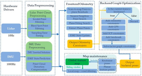
Figure 1.
Algorithm overall flowchart.
3.1. Frontend Odometry
The frontend odometry module is responsible for calculating the relative pose relationship between consecutive LiDAR frames, providing pose constraints between adjacent LiDAR frames. As LOAM-series frontend odometry relies on the computation of point-to-line features [29], and the extraction of line-plane features in solid-state LiDAR is related to the LiDAR’s scanning method. This paper adopts the idea from FastLio, proposing a tightly coupled frontend odometry that does not depend on traditional point cloud curvature calculation for extracting line features [18,30]. The algorithm is modified to suit the rail transportation environment and the requirements of offline map construction.
The algorithm is based on an ESKF filter for the tightly coupled LiDAR-IMU method [30]. During initialization, the system is required to remain stationary for a period, utilizing collected data to initialize the gravity vector, IMU biases, and noise, among other parameters. When the algorithm is running, raw data from the LiDAR are input into the LiDAR point cloud preprocessing module. Invalid points and points in close proximity are filtered out, and the remaining points are sorted based on sampling time in ascending order. This sorting facilitates distortion compensation based on IMU preintegration results. The preintegration method is then used to perform inertial navigation on the raw IMU data. Based on the inertial navigation results, motion distortion in the point cloud is compensated, and the prediction phase of the ESKF filter is executed. The temporal flow of LiDAR and IMU data is illustrated in Figure 2 [20,31].
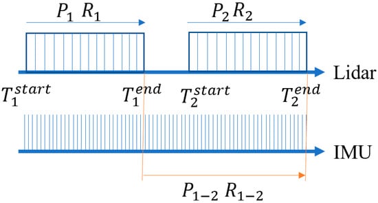
Figure 2.
Schematic diagram of time flow for LiDAR and IMU.
Figure 2 depicts two scans of the LiDAR, denoted as and , with the starting time as the start and the ending time as the end. During a scan, the pose transformation of the LiDAR within the time interval to is represented by and . Therefore, all point clouds within the time interval to are transformed to the moment to compensate for the motion distortion in the original point cloud. Simultaneously, the frontend odometry needs to output the inter-frame pose transformation between two scans. In the prediction phase of the ESKF filter, the inertial navigation results and within the time interval to are directly used as the filter’s prediction input.
The state variables and kinematic equations used in the ESKF filter are represented by Equations (1) and (2), where all variables are denoted with superscript “I” for the IMU coordinate system and “G” for the Earth coordinate system.
—position in the Earth coordinate system; —velocity in the Earth coordinate system; —rotation matrix of the attitude in the Earth coordinate system; —accelerometer measurement; —accelerometer bias; —accelerometer noise; —gravity vector; —gyroscope measurement; —gyroscope bias; —gyroscope noise; —gyroscope bias random walk noise; —accelerometer bias random walk noise.
In the map maintenance module, a sliding window is maintained based on the current position of the LiDAR, and a local map is output for scan-to-map matching. The raw LiDAR point cloud undergoes motion compensation and voxel filtering down-sampling. The ESKF filter establishes the point-to-plane constraint relationship. Using kd-tree nearest-neighbor search, the five nearest points () to the current point (P) are selected from the local map. This decision is primarily based on the structural characteristics of the point cloud within the tunnel environment. Opting for five points in the plane-fitting process ensures accurate fitting of the ground plane and other features present in the tunnel, such as installed signs and road edge planes. Choosing more than five points might result in a scarcity of plane points, leading to significant solving errors, while selecting fewer than five points could result in larger residuals in the fitted plane, causing fitting inaccuracies. The plane equation is then fitted using Principal Component Analysis (PCA) as follows [32]:
Each dimension of the data is subtracted by its mean value. After transformation, the mean value of each dimension becomes zero. Compute the covariance matrix for the three coordinates. The covariance matrix is defined as follows:
where represents the covariance between the and coordinates, and is the variance of the coordinate. The covariance calculation is defined by Equation (4), where are the coordinates of the centered points:
The eigenvalues and eigenvectors of the covariance matrix are computed. The calculated eigenvalues, sorted in descending order, are denoted as , with corresponding eigenvectors . Clearly, the eigenvectors corresponding to the two largest eigenvalues form a set for the plane to be fitted, while represents the normal vector of the fitting plane, with components . If the fitting plane passes through the point , the equation of the fitted plane is given by Equation (5):
The curvature-based feature extraction method has the advantage of rapidly extracting line and surface features, but it is challenging to achieve comprehensive and accurate feature extraction in long tunnel scenarios lacking distinct features. This method is prone to degradation in the driving direction. To prevent the ESKF filter from diverging in scenes with fewer features, a method for constructing plane point constraints is proposed. This method uses the following two conditions to determine whether a point can be used to construct a constraint relationship as a planar point:
1. The distance from each of the five points () to the fitted plane is less than 0.1 m.
2. The threshold is set to , where is the distance from point to the fitted plane, and is the distance from point to the center of the LiDAR. As is much smaller than between any two frames, to filter measurement errors from exceptional plane points, the constructed plane constraint is considered valid only when .
Finally, the ESKF filter is updated based on the point-to-plane residual constraints, and the optimal estimate of the state variables is output as the output of the inter-frame frontend odometry. The covariance matrix is updated, and the ESKF filter is iterated.
3.2. Backend Graph Optimization
In the context of the backend optimization problem based on the pose graph, each node in the factor graph represents a pose to be optimized. The edges between any two nodes represent spatial constraints between the corresponding poses, including relative pose relationships and their associated covariances. The relative pose relationships between nodes can be computed using frontend odometry, IMU pre-integration, frame-to-frame matching, and other methods. Given the utilization of the tightly coupled LiDAR-IMU approach in the frontend odometry, frame-to-frame IMU pre-integration constraints are not employed in the backend optimization.
Addressing the challenges of solving high-dimensional constraints, this paper proposes a framework with high dimensionality and multiple constraints, as illustrated in Figure 1. The framework leverages ESKF in the frontend odometry to provide high-frequency position updates. In the backend, a graph optimization constraint-solving approach is employed, integrating various constraints. The ESKF frontend odometry provides high-frequency position updates, and the backend uses graph optimization constraints that fuse various constraints. The key constraints integrated into the factor graph include frame-to-frame odometry factors, absolute pose factors, ICP factors, and Landmark factors, forming the factor graph depicted in Figure 3. In the optimization process after adding each new keyframe, the initial values for solving are provided by the frontend odometry.
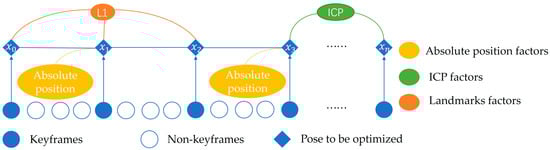
Figure 3.
Algorithm flowchart for backend graph optimization.
To batch optimize historical keyframe poses , this paper employs a factor graph optimization method, where each keyframe pose is a vertex in the graph. Through the computation of frontend odometry and point cloud matching results, edges are constructed between adjacent keyframe poses or any two keyframe poses. Additionally, for extra observations such as absolute pose constraints or Landmark constraints, edges connecting vertices are added to the factor graph.
3.2.1. Frame-to-Frame Odometry
The inter-frame constraints for adjacent keyframes in the backend graph optimization are provided by the frontend odometry module. To select keyframes for optimization, the current frame is compared to the state of the previous keyframe . When the pose change exceeds a threshold, the current frame is chosen as a keyframe. In the factor graph, the newly selected keyframe is associated with the previous state node . LiDAR scans between two keyframes are discarded to maintain a relatively sparse factor graph while balancing map density and memory consumption, suitable for map construction. Ultimately, the relative pose transformation between and is obtained. In practical testing, considering the field of view of the LiDAR and ensuring offline mapping accuracy in degraded scenarios, the thresholds for positional and rotational changes to identify keyframes are set to 0.5 m and 1 degree, respectively.
3.2.2. Absolute Pose Factors
In degraded scenarios, relying solely on long-term pose estimates from IMU and LiDAR will accumulate errors. To address this issue, the backend optimization system needs to incorporate sensors providing absolute pose measurements to eliminate cumulative errors. Absolute pose correction factors mainly include two types:
- 1.
- GPS-Based Factors
Absolute poses are obtained from GPS sensors in the current state and transformed into the local Cartesian coordinate system. As shown in Figure 3, an absolute pose factor has already been introduced at keyframe . After adding new keyframes and other constraints to the factor graph, due to the slow growth of accumulated errors from the frontend odometry, introducing absolute pose constraints too frequently for backend optimization can lead to difficulty in constraint solving and poor real-time algorithm performance. Therefore, a new GPS factor is added to keyframe only when the position change between keyframe and keyframe exceeds a threshold. The covariance matrix of the absolute pose depends on the precision of the sensor used and the quality of satellite signal reception.
- 2.
- Control Point-Based Factors in GPS-Limited Environments
In environments lacking satellite signals, such as tunnels, GPS sensors cannot be directly used for pose correction. In such cases, control points’ absolute coordinates are obtained in advance using surveying equipment like total stations. When the LiDAR moves near the relevant control points, the target perception algorithm outputs the control points’ relative coordinates in the LiDAR coordinate system. Using Equation (6), the LiDAR’s absolute pose coordinates are then determined. The covariance matrix of the absolute pose depends on the covariance of the target positions output by the Kalman tracking algorithm in the perception algorithm.
where —absolute coordinates of the control point; —rotation matrix representing the LiDAR’s pose; —relative coordinates of the control point in the LiDAR coordinate system; —absolute coordinates of the LiDAR.
In the actual process, absolute pose factors are only introduced into the system for global optimization when the pose covariance output by the frontend odometry is significantly larger than the received absolute pose covariance.
3.2.3. ICP Factors
The ICP factor involves solving the relative pose transformation between point clouds corresponding to any two keyframes using the ICP algorithm. In the factor graph shown in Figure 3, when keyframe is added to the factor graph, a set of ICP constraints is constructed between keyframes and . The backend optimization factor graph adds ICP factors in the following two situations:
- 1.
- Loop Closure Detection
When a new keyframe is added to the factor graph, it first searches for the keyframe in the Euclidean space that is closest to . An ICP factor is added to the factor graph only if and are within a spatial distance threshold ∆d and a temporal separation greater than a threshold ∆t. In practical experiments, due to the difficulty of forming loop constraints in the unidirectional movement of subways, loop constraints are constructed in platform areas of both up and down directions on the same route.
- 2.
- Low-Speed or Stationary Conditions
In degraded scenarios, the IMU zero offset estimates in the frontend odometry can accumulate significant errors during prolonged low-speed or stationary vehicle conditions, leading to drift in the frontend odometry. Therefore, additional constraints need to be added in such scenarios to avoid pose drift during prolonged stops. Subway trains typically stop only at platforms in tunnel scenes, where point cloud features are abundant, providing sufficient geometric information for ICP constraint solving. When the system detects low-speed or stationary states, it re-caches every keyframe in this state. Whenever a new keyframe is added to the factor graph, a constraint relationship is established between and the keyframe , which is the furthest in time from the current keyframe.
When the conditions for adding ICP factors are met, the system searches for the n closest keyframes in the historical keyframes to establish a local point cloud map. This local point cloud map is then used for ICP constraint solving with , ultimately obtaining a set of relative pose transformation relationships between and . The covariance matrix of the ICP factor is calculated based on the goodness of fit output during the ICP solving process.
3.2.4. Landmark Factors
The establishment and solving of Landmark factors adopt the Bundle Adjustment (BA) optimization concept commonly used in visual SLAM. As shown in Figure 3, when keyframes , , and all observe the same landmark point , and since the absolute coordinates of remain constant, constraint relationships between —, —, and — can be established based on Equation (7).
where —absolute coordinates of landmark point , not directly solved during the process; —attitude rotation matrix of the LiDAR in keyframe ; —relative coordinates of the landmark point in keyframe in the LiDAR coordinate system; —absolute coordinates of the LiDAR in keyframe .
Therefore, the key to adding Landmark factors lies in how to obtain real-time observations of the position and attitude of the same landmark point. The selection of landmark points is crucial, ensuring continuous observations over a short period and maintaining relatively constant shape and size during the observation to avoid abrupt changes in the object’s center of mass. In urban scenes, road signs are chosen as landmark points, while in tunnel scenes of rail transportation, mileposts alongside the track are selected as landmark points.
3.3. Map Update
After completing the global optimization for each keyframe, it is necessary to update the stored global map based on the optimized keyframe poses. Furthermore, considering the LiDAR’s position in the map, a local feature map is extracted from the global map. This local feature map serves as input to the frontend odometry for scan-to-map matching. In the process of updating the local feature map, this paper implements a position-based sliding window approach. It involves extracting information from the nearest n sub-keyframes to the current LiDAR position, focusing on plane point clouds. Subsequently, the concatenated map undergoes voxel filtering and downsampling to reduce computational load during the matching process.
4. Experimental Results and Discussion
Considering the difficulty in obtaining real-time ground truth poses in the tunnel environment of rail transportation, the proposed offline mapping method with a tightly coupled frontend and graph optimization backend was experimentally validated in both urban road outdoor scenes and rail transportation scenes.
Taking into account the challenge of obtaining real-time ground truth poses in the tunnel environment of rail transit, the mapping method proposed in this paper, featuring a tightly coupled frontend and a graph optimization backend, has not only been experimentally validated in subway scenarios but has also been compared with RTK+IMU integrated navigation in industrial park building obstruction environments. This additional comparison aims to further assess the cumulative error of the proposed method.
4.1. Experimental Equipment
The mapping data acquisition system uses the RS-LiDAR-M1, an automotive-grade solid-state LiDAR. It operates with a 905 nm wavelength laser, providing a maximum range of 200 m and an accuracy ranging within ±5 cm. The LiDAR has a horizontal field of view of 120° with a resolution of 0.2°, a vertical field of view of 25° with a resolution of 0.2°, and the ability to output up to 750,000 points per second in single-echo mode. The selected IMU model is the STIM300, with an accelerometer resolution of 1.9 μg, bias instability of 0.05 mg, gyroscope resolution of 0.22°/h, and gyroscope bias instability of 0.3°/h. The sensor installation and layout diagrams for the subway environment and the industrial park environment are illustrated in Figure 4a,b, respectively.
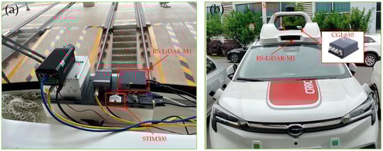
Figure 4.
Physical installation and arrangement of sensors. (a) Sensors on the train. (b) Sensors on the autonomous driving platform vehicle.
4.2. Subway Tunnel Scene
Given the degraded nature of tunnel scenes, where the number of feature points in LiDAR point clouds for matching is limited and prone to misalignment, the covariance of point-to-plane residuals needs to be increased when detecting degradation in the frontend odometry. Simultaneously, in the ESKF filter, the covariance of IMU inertial solutions is reduced. During the backend optimization process, considerations include addressing drift in low-speed stationary train scenarios and selecting appropriate landmarks.
4.2.1. Low-Speed Stationary Scenario
During the map data collection process, the train normally stops in the platform area, which is rich in features. There are enough planar feature points for inter-frame matching and the addition of ICP constraints, as shown in Figure 5. Features such as the tunnel wall and the train stop sign can be used for matching.
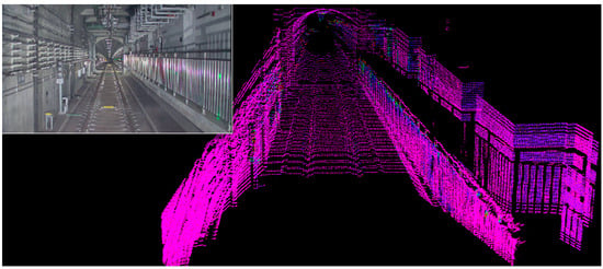
Figure 5.
Point cloud effect in normal station platform parking (underground subway parking).
However, in situations where the train is stationary in the curved section of the tunnel or when the ICP factor is turned off in the algorithm, significant drift can occur when there is a large change in train speed during stationary periods, as illustrated in Figure 6. The output trajectory exhibits a backward movement when the train is stationary, emphasizing the need to avoid abrupt acceleration, deceleration, and stops in severely degraded scenes during map data collection.
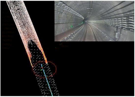
Figure 6.
Drift in train parking trajectory in tunnel. The trajectory exhibits a phenomenon of moving backward within the red circle.
4.2.2. Landmark Selection
Due to the limited number of extractable landmarks in subway tunnel scenes, the intensity information of point clouds and the arrangement of signs inside the tunnel are considered. The recognition of hundred-meter markers is chosen as a landmark for constraints, as shown in Figure 7. Since the hundred-meter markers are made of metal, the intensity information is substantial, allowing for direct extraction of relevant point clouds based on intensity filtering. The final step involves extracting the centroid coordinates of the relevant point clouds and incorporating them into the factor graph for optimization and solving.
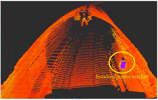
Figure 7.
Detection of hundred-meter markers in the tunnel.
4.2.3. Landmark Selection
In the subway tunnel scenario, quantitative analysis is challenging due to the lack of ground truth. Therefore, the evaluation is based on multiple data collections in the same subway tunnel scene, comparing the consistency of trajectories and focusing on the assessment in platform areas and tunnel sections. The three-dimensional point cloud results of the mapping are shown in Figure 8 and Figure 9. In the original point cloud, the tracks and tunnel walls are clearly visible, indicating that our algorithm achieves high accuracy in local areas.
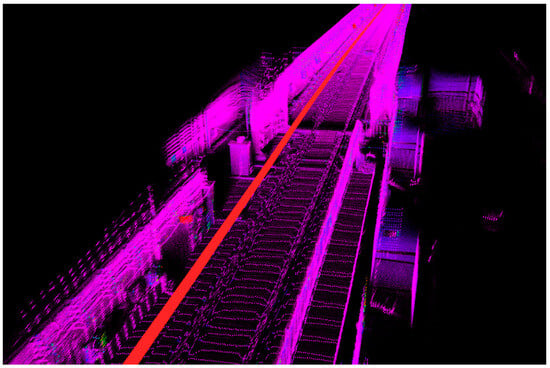
Figure 8.
Mapping results of subway tunnel platform.
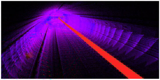
Figure 9.
Mapping results of subway tunnel curve.
To evaluate the consistency of data collected, we used the trajectory from the initial mapping session as ground truth and analyzed the error in the overlap between the trajectories of subsequent mapping sessions. To address the challenge of ensuring a consistent starting point for each data collection, we utilized the evo tool to align the trajectories of multiple sessions, as illustrated in Figure 10. Developed by Michael Grupp, the evo tool is a Python package designed for assessing odometry and SLAM results. It provides functionalities, including aligning and comparing trajectories, computing errors, and generating visualizations, facilitating a comprehensive evaluation of localization and mapping performance. The maximum Absolute Pose Error (APE) recorded was 0.1 m, with an average of 0.04 m and a Root Mean Square Error (RMSE) of 0.05 m.
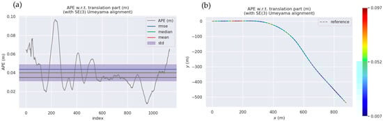
Figure 10.
Consistency results for data collected at different times in the same subway tunnel scene. (a) APE, RMSE, median, mean, std. (b) APE in the xy-plane.
Additionally, due to the significant distance between subway stations in tunnels, mapping within the tunnels involves a higher number of keyframes and the use of unsampled point clouds for stitching. This results in elevated computational and memory requirements for offline map construction. To address these challenges, we propose a multi-map stitching approach, creating a map for each platform interval and then concatenating maps from multiple intervals. Since subway platforms exhibit rich features, we choose to stop and concatenate maps at these locations. We record the last frame pose of the previous map as the initial pose for the current map and manually adjust constraints at the platform using the interactive SLAM method to reduce cumulative errors [33].
4.3. Industrial Park Building Obstructed Environment
To simulate tunnel environments as much as possible and provide a comparison with RTK + IMU combined navigation positioning as ground truth, the experiments were conducted in an industrial park scene. In this scene, the LiDAR’s horizontal field of view was obstructed by buildings, but it still received satellite positioning signals. The sensors were mounted on the roof of the vehicle, as shown in Figure 4a. The addition of GPS factors in the backend optimization was constrained only at the starting and ending positions of the trajectory. The ground truth trajectory during mapping was provided by a high-precision RTK + IMU combined navigation device, and the established point cloud map is shown in Figure 11. In the 3D point cloud map, vehicles and signs are clearly visible, indicating that our algorithm has high precision in local areas.
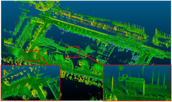
Figure 11.
Point cloud map in an industrial park scene. The red boxes are displays that have been partially enlarged.
We compared the keyframe trajectories output by our algorithm after backend optimization with the ground truth provided by the combined inertial navigation (RTK + IMU) to quantitatively evaluate the accuracy of the mapping algorithm. The trajectory curves in the x, y, and z directions are plotted in Figure 12. The blue curve represents the ground truth trajectory provided by the RTK + IMU combined navigation device, and the gray dashed line represents the keyframe trajectory output by the mapping algorithm. It can be observed that the trajectory error is small in the horizontal direction, while in the vertical direction, the altitude error from the RTK + IMU combined navigation is relatively larger compared to the errors in the horizontal direction. The altitude trajectory curve output by our mapping algorithm is smoother and generally consistent with the ground truth trend.
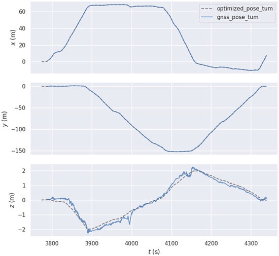
Figure 12.
Position comparison in x, y, and z directions.
In the quantitative assessment of algorithm accuracy, we selected the APE of the trajectory as the evaluation metric, focusing only on position error and neglecting orientation error. Therefore, the calculated APE results are in units of meters. The computed APE results are shown in Figure 13 and Figure 14.
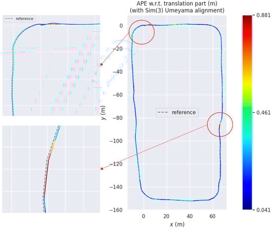
Figure 13.
APE trajectory curve. Red arrows and circles are employed for locally enlarged displays.
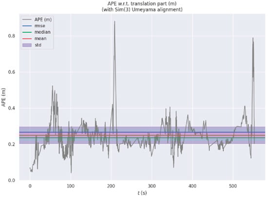
Figure 14.
APE statistical results.
Due to the inclusion of GPS factors only at the starting and ending points during the backend optimization process and the use of trajectory alignment methods, the APE is larger at the starting point. The increased error at turning points is attributed to calibration errors between the LiDAR and IMU, with the calibration error causing more noticeable APE as the turning speed increases. Additionally, partial occlusion by buildings results in a decrease in the accuracy of the RTK + IMU combined navigation used as ground truth, further contributing to an increase in APE values.
The statistical results of APE in Figure 14 are as follows: maximum value (max) = 0.88 m, minimum value (min) = 0.04 m, mean = 0.23 m, and root mean square error = 0.26 m. The quantitative analysis results demonstrate the algorithm’s high trajectory accuracy.
4.4. Discussion
In comparison to mainstream SLAM algorithms, such as Fast-LIO [18,30], our proposed frontend odometer and backend optimization framework focuses on mapping. This approach addresses the challenges of pose estimation in degraded tunnel environments. The design of our framework is specifically tailored to the structural characteristics of tunnel scenes and the operational requirements of trains in tunnel intervals, resulting in high-precision point cloud construction.
In the subway mapping and localization process, the absence of a GNSS as ground truth may result in cumulative errors. Additionally, during the initial wake-up phase of the train, without GNSS signals for providing the initial position, the system faces challenges in initialization.
To address these limitations, we propose utilizing visual recognition of mileposts and their unique identifiers alongside the tracks. The unique identifiers of mileposts can be leveraged for calibrating subway positions. Moreover, incorporating visual methods can enhance the success rate of initialization, thus increasing the robustness of the subsequent localization system.
5. Conclusions
In this paper, we proposed a high-precision point cloud map construction method based on LiDAR and IMU. The approach utilizes a tightly coupled frontend odometry with an ESKF for inter-frame pose estimation, and a backend global pose optimization employing graph optimization theory. Absolute pose factors, ICP factors, and Landmark factors are incorporated into the optimization process based on real-world scenarios. In the context of long urban subway tunnels, the algorithm introduces detection for degraded scenes in the frontend odometry and emphasizes the inclusion of ICP factors in low-speed stationary situations and the selection of Landmark points in the backend graph optimization.
The algorithm’s performance is evaluated by assessing the consistency of trajectories using different data collected on the same route, with a particular focus on platform and tunnel areas. The trajectory alignment error is consistently below 0.11 m. No degradation anomalies were observed throughout the entire tunnel section. Additionally, in the experimental setup in an industrial park scenario, the optimized trajectory is compared with the ground truth provided by the integrated navigation system, yielding an RMSE of 0.26 m for the APE and an accumulated error of less than 0.2%. It is evident that the proposed algorithm achieves high-precision map construction in tunnels and obstructed environments. The next step will be to address the pose initialization problem in degraded environments, particularly in long tunnel scenarios.
Author Contributions
Conceptualization, C.L. and W.P.; methodology, C.L. and W.P.; software, W.H. and F.W.; validation, W.P. and W.H.; formal analysis, W.H.; investigation, C.L. and X.Y.; data curation, C.Y. and Q.W.; writing—original draft preparation, W.P. and W.H.; writing—review and editing, W.H. and X.Y.; visualization, X.Y. and F.W. All authors have read and agreed to the published version of the manuscript.
Funding
This work was funded by the National Key Research and Development Project of China (2022YFB4300400).
Data Availability Statement
Data are contained within the article.
Acknowledgments
All authors would like to thank the editors and anonymous reviewers for their valuable comments and suggestions, which improved the quality of the manuscript. Additionally, we would like to express our gratitude to Shanghai Huace Navigation Technology Co., Ltd. for their technical assistance and support during testing.
Conflicts of Interest
All authors are employed by the company CRRC Zhuzhou Institute Co., Ltd. All authors declare that the research was conducted in the absence of any commercial or financial relationships that could be construed as a potential conflict of interest.
References
- Sun, H.; Xu, Z.; Yao, L.; Zhong, R.; Du, L.; Wu, H. Tunnel monitoring and measuring system using mobile laser scanning: Design and deployment. Remote Sens. 2020, 12, 730. [Google Scholar] [CrossRef]
- Foria, F.; Avancini, G.; Ferraro, R.; Miceli, G.; Peticchia, E. ARCHITA: An innovative multidimensional mobile mapping system for tunnels and infrastructures. MATEC Web Conf. 2019, 295, 01005. [Google Scholar] [CrossRef]
- Cheng, R.; Song, Y.; Chen, D.; Chen, L. Intelligent localization of a high-speed train using LSSVM and the online sparse optimization approach. IEEE Trans. Intell. Transp. Syst. 2017, 18, 2071–2084. [Google Scholar] [CrossRef]
- Wu, Y.; Weng, J.; Tang, Z.; Li, X.; Deng, R.H. Vulnerabilities, attacks, and countermeasures in balise-based train control systems. IEEE Trans. Intell. Transp. Syst. 2016, 18, 814–823. [Google Scholar] [CrossRef]
- Wang, Z.; Yu, G.; Zhou, B.; Wang, P.; Wu, X. A train positioning method based-on vision and millimeter-wave radar data fusion. IEEE Trans. Intell. Transp. Syst. 2021, 23, 4603–4613. [Google Scholar] [CrossRef]
- Otegui, J.; Bahillo, A.; Lopetegi, I.; Diez, L.E. Evaluation of experimental GNSS and 10-DOF MEMS IMU measurements for train positioning. IEEE Trans. Instrum. Meas. 2018, 68, 269–279. [Google Scholar] [CrossRef]
- Buffi, A.; Nepa, P. An RFID-based technique for train localization with passive tags. In Proceedings of the IEEE International Conference on RFID (RFID), Phoenix, AZ, USA, 9–11 May 2017; pp. 155–160. [Google Scholar]
- Daoust, T.; Pomerleau, F.; Barfoot, T.D. Light at the end of the tunnel: High-speed lidar-based train localization in challenging underground environments. In Proceedings of the 2016 13th Conference on Computer and Robot Vision (CRV), Victoria, BC, Canada, 1–3 June 2016. [Google Scholar]
- Liu, H.; Pan, W.; Hu, Y.; Li, C.; Yuan, X.; Long, T. A Detection and Tracking Method Based on Heterogeneous Multi-Sensor Fusion for Unmanned Mining Trucks. Sensors 2022, 22, 5989. [Google Scholar] [CrossRef]
- Pan, W.; Fan, X.; Li, H.; He, K. Long-Range Perception System for Road Boundaries and Objects Detection in Trains. Remote Sens. 2023, 15, 3473. [Google Scholar] [CrossRef]
- Wang, J.; Chen, W.; Weng, D.; Ding, W.; Li, Y. Barometer assisted smartphone localization for vehicle navigation in multilayer road networks. Measurement 2023, 211, 112661. [Google Scholar] [CrossRef]
- Gao, F.; Wu, W.; Gao, W.; Shen, S. Flying on point clouds: Online trajectory generation and autonomous navigation for quadrotors in cluttered environments. J. Field Robot. 2019, 36, 710–733. [Google Scholar] [CrossRef]
- Wang, J.; Weng, D.; Qu, X.; Ding, W.; Chen, W. A Novel Deep Odometry Network for Vehicle Positioning Based on Smartphone. IEEE Trans. Instrum. Meas. 2023, 72, 2505512. [Google Scholar] [CrossRef]
- Ye, H.; Chen, Y.; Liu, M. Tightly coupled 3d lidar inertial odometry and mapping. In Proceedings of the IEEE International Conference on Robotics and Automation (ICRA), Montreal, QC, Canada, 20–24 May 2019. [Google Scholar]
- Zhao, S.; Fang, Z.; Li, H.; Scherer, S. A Robust Laser-Inertial Odometry and Mapping Method for Large-Scale Highway Environments. In Proceedings of the 2019 IEEE/RSJ International Conference on Intelligent Robots and Systems (IROS), Macau, China, 4–8 November 2019; pp. 1285–1292. [Google Scholar] [CrossRef]
- Qin, T.; Li, P.; Shen, S. VINS-Mono: A Robust and Versatile Monocular Visual-Inertial State Estimator. IEEE Trans. Robot. 2018, 34, 1004–1020. [Google Scholar] [CrossRef]
- Liu, X.; Zhang, F.Z. Extrinsic calibration of multiple lidars of small fov in targetless environments. IEEE Robot. Autom. Lett. 2021, 6, 2036–2043. [Google Scholar] [CrossRef]
- Xu, W.; Zhang, F. Fast-lio: A fast, robust lidar-inertial odometry package by tightly-coupled iterated kalman filter. IEEE Robot. Autom. Lett. 2021, 6, 3317–3324. [Google Scholar] [CrossRef]
- Liu, Z.; Zhang, F. BALM: Bundle adjustment for lidar mapping. IEEE Robot. Autom. Lett. 2021, 6, 3184–3191. [Google Scholar] [CrossRef]
- Lin, J.; Zhang, F. Loam livox: A fast, robust, high-precision lidar odometry and mapping package for lidars of small fov. In Proceedings of the 2020 IEEE International Conference on Robotics and Automation (ICRA), Paris, France, 31 May–31 August 2020; pp. 3126–3131. [Google Scholar]
- Lin, J.; Zhang, F. R 3 LIVE: A Robust, Real-time, RGB-colored, LiDAR-Inertial-Visual tightly-coupled state Estimation and mapping package. In Proceedings of the IEEE International Conference on Robotics and Automation (ICRA), Philadelphia, PA, USA, 23–27 May 2022. [Google Scholar]
- Bao, Z.; Hossain, S.; Lang, H.; Lin, X. A review of high-definition map creation methods for autonomous driving. Eng. Appl. Artif. Intell. 2023, 122, 106125. [Google Scholar] [CrossRef]
- Zhou, H.; Yao, Z.; Lu, M. Uwb/lidar coordinate matching method with anti-degeneration capability. IEEE Sens. J. 2020, 21, 3344–3352. [Google Scholar] [CrossRef]
- Zhuang, Y.; Sun, X.; Li, Y.; Huai, J.; Hua, L.; Yang, X.; Cao, X.; Zhang, P.; Cao, Y.; Qi, L.; et al. Multi-sensor integrated navigation/positioning systems using data fusion: From analytics-based to learning-based approaches. Inf. Fusion 2023, 95, 62–90. [Google Scholar] [CrossRef]
- Heirich, O.; Robertson, P.; Strang, T. RailSLAM—Localization of Rail Vehicles and Mapping of Geometric Railway Tracks. In Proceedings of the IEEE International Conference on Robotics and Automation (ICRA), Karlsruhe, Germany, 6–10 May 2013. [Google Scholar]
- Wang, Y.; Song, W.; Lou, Y.; Zhang, Y.; Huang, F.; Tu, Z.; Liang, Q. Rail Vehicle Localization and Mapping with LiDAR-Vision-Inertial-GNSS Fusion. IEEE Robot. Autom. Lett. 2022, 7, 9818–9825. [Google Scholar] [CrossRef]
- Tschopp, F.; Schneider, T.; Palmer, A.W.; Nourani-Vatani, N.; Cadena, C.; Siegwart, R.; Nieto, J. Experimental comparison of visual-aided odometry methods for rail vehicles. IEEE Robot. Autom. Lett. 2019, 4, 1815–1822. [Google Scholar] [CrossRef]
- Wang, Y.; Song, W.; Lou, Y.; Huang, F.; Tu, Z.; Zhang, S. Simultaneous Location of Rail Vehicles and Mapping of Environment with Multiple LiDARs. arXiv 2021, arXiv:2112.13224. [Google Scholar]
- Shan, T.; Englot, B. LeGO-LOAM: Lightweight and Ground-Optimized Lidar Odometry and Mapping on Variable Terrain. In Proceedings of the IEEE/RSJ International Conference on Intelligent Robots and Systems (IROS), Madrid, Spain, 1–5 October 2018; IEEE: Piscataway, NJ, USA, 2018. [Google Scholar]
- Xu, W.; Cai, Y.; He, D.; Lin, J.; Zhang, F. Fast-lio2: Fast direct lidar-inertial odometry. IEEE Trans. Robot. 2022, 38, 2053–2073. [Google Scholar] [CrossRef]
- Fan, X.; Chen, Z.; Liu, P.; Pan, W. Simultaneous Vehicle Localization and Roadside Tree Inventory Using Integrated LiDAR-Inertial-GNSS System. Remote Sens. 2023, 15, 5057. [Google Scholar] [CrossRef]
- Feng, C.; Taguchi, Y.; Kamat, V.R. Fast plane extraction in organized point clouds using agglomerative hierarchical clustering. In Proceedings of the IEEE International Conference on Robotics and Automation (ICRA), Hong Kong, China, 31 May–7 June 2014. [Google Scholar]
- Koide, K.; Miura, J.; Yokozuka, M.; Oishi, S.; Banno, A. Interactive 3D graph SLAM for map correction. IEEE Robot. Autom. Lett. 2020, 6, 40–47. [Google Scholar] [CrossRef]
Disclaimer/Publisher’s Note: The statements, opinions and data contained in all publications are solely those of the individual author(s) and contributor(s) and not of MDPI and/or the editor(s). MDPI and/or the editor(s) disclaim responsibility for any injury to people or property resulting from any ideas, methods, instructions or products referred to in the content. |
© 2024 by the authors. Licensee MDPI, Basel, Switzerland. This article is an open access article distributed under the terms and conditions of the Creative Commons Attribution (CC BY) license (https://creativecommons.org/licenses/by/4.0/).