Abstract
Reanalysis datasets provide a reliable reanalysis of climate input data for hydrological models in regions characterized by limited weather station coverage. In this paper, the accuracy of precipitation, the maximum and minimum temperatures of four reanalysis datasets, the China Meteorological Assimilation Driving Datasets for the SWAT model (CMADS), time-expanded climate forecast system reanalysis (CFSR+), the European Centre for Medium-Range Weather Forecast Reanalysis (ERA). and the China Meteorological Forcing Dataset (CMFD), were evaluated by using data from 28 ground-based observations (OBs) in the Source of the Yangtze and Yellow Rivers (SYYR) region and were used as input data for the SWAT model for runoff simulation and performance evaluation, respectively. And, finally, the CMADS was optimized using Integrated Calibrated Multi-Satellite Retrievals for Global Precipitation Measurement (AIMERG) data. The results show that CMFD is the most representative reanalysis data for precipitation characteristics in the SYYR region among the four reanalysis datasets evaluated in this paper, followed by ERA5 and CFSR, while CMADS performs satisfactorily for temperature simulations in this region, but underestimates precipitation. And we contend that the accuracy of runoff simulations is notably contingent upon the precision of daily precipitation within the reanalysis dataset. The runoff simulations in this region do not effectively capture the extreme runoff characteristics of the Yellow River and Yangtze River sources. The refinement of CMADS through the integration of AIMERG satellite precipitation data emerges as a potent strategy for enhancing the precision of runoff simulations. This research can provide a reference for selecting meteorological data products and optimization methods for hydrological process simulation in areas with few meteorological stations.
1. Introduction
Located in Northwest China’s Qinghai Province, the Source of the Yangtze and Yellow Rivers (SYYR) is the home to the headstreams of China’s two great rivers, the Yangtze and Yellow river, which provide water resources for the country’s natural ecosystems and a population exceeding hundreds of millions [1]. This assumes indispensable functions in the preservation of water, regulation of runoff, and the sustenance of ecological diversity [2,3,4]. Runoff, a pivotal facet of the hydrological cycle, exerts consequential effects on both the regional hydrological dynamics and holds substantial implications for water security and ecological well-being in downstream regions [5,6]. Therefore, the large-scale simulation or prediction of runoff within the SYYR region holds significance in advancing our comprehension of surface water availability and management [7].
Watershed hydrological models have gained extensive utilization in the simulation and prediction of runoff processes and are now mainly classified into the lumped hydrological models, and the semi-distributed and distributed models. Sun et al. [8] applied the calibrated lumped Xin’anjiang model for flood forecasting in the Shaowu basin. Dal et al. [9] used the semi-distributed hydrological model to investigate the control of spatial variability of runoff by the main river channel in the Thur basin, Switzerland. Liu et al. [10] used the distributed hydrological model based on hydrothermal coupling considering glaciers and permafrost to model the hydrological processes associated with the water cycle in the Niyang River basin, located on the Qinghai–Tibet Plateau. Compared with these models, the advantage of the Soil and Water Assessment Tool (SWAT) model is that it not only has a strong physical basis, which can integrate geographic information systems (GISs), remote sensing (RS), and digital elevation models (DEMs), but also has a good user interface, strong spatial data management, organization, analysis, and presentation capabilities. At present, the SWAT model has experienced growing adoption among hydrologists and water resource managers for evaluating the influence of anthropogenic activities and climatic variations on water resources [11]. However, a large amount of basic data are required for the operation of the SWAT model, which includes four main components: DEM data, land use data, soil data, and meteorological data. Over the years, the data quality of DEMs, land use, and soil datasets has witnessed substantial improvement owing to the swift evolution in remote sensing techniques and advancements in data classification methodologies [12]. The availability and quality of meteorological data may be critical to the results of simulations, but dense meteorological observatories are expensive to maintain and not easily accessible [13]. However, the insufficiency of weather stations and meteorological data, coupled with the absence of comprehensive, long-term time series datasets, characterizes the data limitations within the SYYR region [14].
With the advancement and development of satellite and ground-based observation technologies, an increasing number of meteorological data products are available for researchers to share and use. In particular, the precipitation data, which are the most important data driving hydrological models, are available in a wide range of options. In a review published in the Reviews of Geophysics, Sun et al. [15] delineated intricate details pertaining to data sources and estimation methodologies for approximately 30 extant global precipitation datasets, derived from gauge, satellite-related, and reanalysis datasets. It is worth highlighting that reanalysis datasets exhibit heightened variability compared to other dataset categories. Simultaneously, the extent of variability in precipitation estimates varies across different geographical regions However, as an important part of the “China Water Tower”, the SYYR region is mainly recharged by natural precipitation and glacial meltwater. In the context of continued global warming, the increasing share of glacial meltwater in water recharge indicates the necessity of enhancing the impacts of temperature on runoff in the SYYR region; taking into account natural precipitation. The significance of the reanalyzed dataset is underscored by its comprehensive incorporation of intricate precipitation data and a multitude of climatic variables, encompassing temperature, solar radiation, and wind speed. Of particular relevance to the SYYR area are precipitation and temperature factors. In comparison to alternative climate products, these datasets comprehensively fulfill our requirements for runoff simulation employing the SWAT model.
Reanalysis datasets denote gridded datasets characterized by spatial and temporal integrity, generated through weather simulation models extrapolating from observed data [13]. They combine satellite data with observational data to represent observed weather as accurately as possible on a continuous time and space scale. Numerous meteorological reanalysis data products have been employed in the realm of hydrological modeling, including the CFSR, one of the preeminent reanalysis climate products utilized in SWAT modeling, contributing about 40% to publications, and CMADS. Although the latter exclusively encompasses the East Asian region, with freely accessible data limited to the temporal span from 2008 to 2018, it still contributes about 13% to publications [16]. In addition, other global reanalysis products used in SWAT include the European Centre for Medium-Range Weather Forecast ReAnalysis (ERA) and the Climatic Research Unit (CRU). Reanalysis datasets usually provide a more accurate representation of weather conditions at the basin or regional scale, but given that the reanalysis system is constituted by a background forecast model and a data assimilation process, their data quality depends to some extent on the observed data used in the reanalysis system [17]. Consequently, in some cases, the reanalysis dataset is not matched by the actual weather conditions in the region. Eini et al. [13] evaluated precipitation data from five reanalysis datasets within the CRU and CFSR in a semi-arid basin and simulated the local hydrology separately and concluded that reanalysis precipitation is a valid alternative for hydrological modeling in semi-arid basins. Ndhlovu et al. [18] utilized gridded climate data in the context of hydrological modeling within the Zambezi River Basin, located in Southern Africa, and showed that the CFSR has a satisfactory hydrological modeling result for this region. However, preceding studies frequently focus solely on evaluating the precision of monthly precipitation, overlooking the evaluation of the precision of daily precipitation data essential for hydrological modeling as mandated by the SWAT model. It also requires an accurate assessment because of the effect of alpine temperature on regional hydrology. Therefore, a comprehensive evaluation of the regional precision of reanalysis data must be an obligatory prerequisite preceding their incorporation into hydrological modeling [13].
Considering the suitability of meteorological reanalysis products across temporal and spatial dimensions, coupled with the availability of data, this paper selects CFSR and CMADS, which are used in hydrological modeling, the regularly updated ERA5 at a global scale, and the China Meteorological Forcing Dataset (CMFD), which is a mainstream Chinese gridded observation. Subsequently, an evaluation is conducted on the efficacy of the CFSR, CMADS, CMFD, and ERA precipitation and temperature datasets within the SYYR region. These datasets are subsequently employed in conjunction with the SWAT model for hydrological simulations in the region, aiming to discern the reanalysis dataset that yields optimal performance in the hydrological modeling context. Section 2 provides a comprehensive overview of the study area, encompassing details on data sources, statistical methodologies, and hydrological models employed in the research. Section 3 offers an in-depth analysis of the performance of the reanalysis dataset, encompassing statistical evaluations and hydrological modeling assessments. Section 4 delves into the underlying factors contributing to the varied applicability of reanalysis data within the SYYR region, elucidating optimization methodologies specific to CMADS. The study culminates in Section 5 with the presentation of key findings and conclusions.
2. Materials and Methods
2.1. Study Area
“Situated on the Tibetan Plateau (TP), the geographic expanse spans approximately 30.53 × 10⁴ km2 within the southern confines of Qinghai province. This area encompasses both the Yangtze River source region and the Yellow River source region, as shown in Figure 1. The Yangtze River source is bounded by the confluence of the Batang River, located between the Kunlun and Tanggula ranges in the heart of the TP covering a watershed area of about 16.11 × 10⁴ km2. With its vast expanse of glaciers, snow-capped peaks, rivers, lakes, and wetlands, this region plays a crucial role as a primary hydrological reservoir. Serving as a vital water source for the Yangtze River basin, the runoff from the Yangtze River source region constitutes approximately 25% of the entire water volume of the Yangtze River” [19]. The term ‘Yellow River source’ designates the region within the Yellow River basin situated upstream of the Longyangxia Reservoir, located in the northeastern segment of the Tibetan Plateau, encompassing a watershed area spanning approximately 14.42 × 10⁴ km2. Despite its modest physical footprint, the Yellow River source exhibits an intricate network of water systems, serving as a vital water catchment in China. Notably, the runoff originating from this source contributes to over 40% of the entire Yellow River basin, establishing it as a substantial component of China’s water tower [20]. In this research, the SYYR region is divided into 54 sub-basins by the SWAT model, as shown Figure 1b.
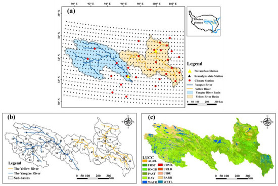
Figure 1.
(a) Study area of the source of the Yangtze and Yellow Rivers: the main river, main tributaries, climate stations, reanalysis data stations, and streamflow stations; (b) the delimitation of the sub-basins with the SWAT model and the numbers are sub-basin numbers; (c): land use types in 2010 (AGRL: agricultural land; FRST: forest-mixed; RNGB: shrubbery; PAST: pasture; HAY: hay; WATR: water; URML: residential area (medium density); URLD: residential area (low density); UIDU: industrial land; BARR: barren; WETL: wetlands).
2.2. Data Sources and Processing
CFSR, CMADS V1.0 (2008–2018) [21], CMFD, and ERA5 were designated as the reanalysis datasets that scrutinize the accuracy of precipitation and temperature (both maximum and minimum) in comparison to observations. Then, they were used as input data for the hydrological simulations. It is imperative to highlight that the CFSR(SWAT) [22] dataset, accessible via the SWAT website, received updates only until July 2014. This limitation compromises its adequacy for fulfilling the contemporary demands of scientific research presentations. In this study, tools such as Matlab2022b and python3.10 were used to connect the NCEP Climate Prediction System version 2 (CFSv2) 6 h product to the CFSR dataset, and updated the CFSR dataset to 2018, the same period as CMADS V1.0. This paper encompasses ground-based observational meteorological data (OBS) utilized for assessing the precision of reanalysis data. Additionally, it includes the DEM data, land use data, and soil data essential for runoff simulation using the SWAT model, along with the hydrological observations required for the calibration process. In addition, the required data include AIMERG [23], the satellite precipitation data needed to optimize CMADS. Detailed information such as the source of the above data can be found in Table 1.

Table 1.
Foundational details pertaining to the datasets employed in this study.
2.3. SWAT Model
The SWAT model, derived from the Simulator for Water Resources in Rural Basins (SWRRB) model, is a semi-distributed hydrological model encompassing three primary sub-modules designed for applications in hydrology, soil erosion, and pollution load assessment [24,25]. Since its development, the model has undergone ongoing refinement, and its efficacy in simulating and forecasting runoff and sediment dynamics has garnered global recognition through widespread utilization and validation.
2.3.1. Hydrological Cycle Processes in SWAT Model
The process of the hydrological cycle follows the principle of water balance. A fraction of the precipitation is intercepted and retained by the vegetative canopy, while the remaining portion impinges upon the soil surface. Subsequently, a segment of the water at the soil surface undergoes infiltration into the soil profile, contributing to the generation of surface runoff, which then converges into the river system. Then, part of the infiltrated water will remain in the soil and evaporate, and others will flow into the surface water system via underground channels [26,27], the formula is as follows:
SWt denotes the final soil water content, SW0 represents the initial soil water content on day ‘i’, where ‘t’ denotes the temporal dimension in days. The variables Rday, Wy, Qsurf, Ea, Wseep, and Qgw, correspondingly, signify the daily quantities of precipitation, snowmelt, surface runoff, evapotranspiration, percolation, and return flow on day ‘i’, with all measurements expressed in millimeters.
2.3.2. Snowmelt Processes in SWAT Model
The SWAT employs a temperature index-based methodology for the estimation of snowmelt processes. The dynamics of snowmelt are intricately influenced by both atmospheric and snowpack temperatures, the rate of melting, and the spatial extent of snow coverage. Within this framework, the model treats the resultant melted snow as akin to rainfall, facilitating the computation of runoff and percolation. The quantification of snowmelt is derived through a linear function, wherein it is expressed as a function of the disparity between the average maximum air temperature associated with the snowpack and a user-defined threshold denoting the temperature conducive to snowmelt.
SNOWmelt represents the daily volume of snowmelt (mm H2O), fmelt denotes the snowmelt factor (mm H2O/°C-day), SNOWcov signifies the proportion of Hydrologic Response Units characterized by snow cover, Tsnow represents the temperature of the snowpack (°C), Tmax corresponds to the maximum temperature (°C), and Tmelt is the temperature threshold indicative of snowmelt initiation (°C).
2.3.3. Model Setup
The simulation of the source basin was executed utilizing the ArcSWAT interface designed for SWAT2009. In the source regions of the Yellow River and the Yangtze River, a single basin outlet is concurrently identified, and the entire basin is delineated into 54 sub-basins using a DEM. In order to optimize both the precision of model computation and computational efficiency, a total of 695 Hydrologic Response Units (HRUs) were generated. The delineation of these HRUs was contingent upon the predominant land use, soil characteristics, and slope, with respective thresholds of 10%, 15%, and 10% being applied.
2.4. Statistical Measures
2.4.1. Validation Strategies
The evaluation of the reanalysis datasets was divided into two main aspects: (1) Climatic aspects—evaluating the accuracy of four reanalysis datasets in terms of precipitation, maximum and minimum temperatures in time (daily/monthly/annual), and space by using OBS data. (2) Hydrological aspects—the comparison of runoff data obtained from four reanalysis datasets and the OBS data-driven SWAT model to analyze their performance in a runoff simulation. As reanalysis datasets are grid data products while OBS data are point data, so the spatial matching between the two kinds of data is a critical aspect. According to Pombo et al. [28] and Tan et al. [29], there are two main approaches to solving the spatial matching problem. To achieve grid-to-point conversion, one approach is to calculate the meteorological indicators corresponding to the location of the actual meteorological station in the reanalysis dataset by simple averaging; the other is to use interpolation to convert points to a grid based on the actual meteorological station locations. In this paper, we choose to calculate the precipitation, maximum temperature, and minimum temperature of four reanalysis datasets at the corresponding points of OBSs using the inverse distance weighting method by comparing the results obtained by the two methods of interpolation and simply averaging them. As for the evaluation of reanalysis datasets, only grids covering at least one OBS site were considered, otherwise, they were excluded from the evaluation.
2.4.2. Validation Metrics
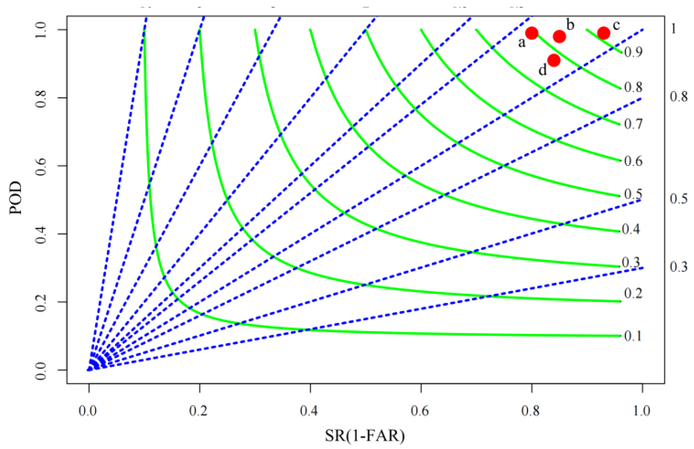
Taylor diagrams serve as a tool for evaluating the performance of four distinct reanalysis datasets of climate information in comparison to observational data. In a Taylor diagram, the correlation coefficient (CC), standard deviation (STD), and root mean square error (RMSD) of the reanalysis climate data are related to the observations by a cosine relationship. This was employed for the evaluation of the precision of precipitation, maximum temperature, and minimum temperature within the reanalysis datasets relative to OBS data. The latter had been extensively utilized in prior research endeavors for the meticulous assessment of gridded climate products [30,31,32]. In addition, three categories of statistical indicators, the Probability of Detection (POD), False Alarm Rate (FAR), and Critical Success Index (CSI), were used to assess the consistency of daily precipitation data with actual precipitation events in the reanalysis data, which can be represented in the performance diagram. POD and FAR metrics quantify the proportions of correctly and incorrectly identified precipitation events relative to the total precipitation occurrences, respectively. Meanwhile, CSI assesses the comprehensive ratio of both precipitation and non-precipitation days detected by the reanalysis data. Within the Taylor diagram, proximity to the ‘observed’ point along the x-axis signifies heightened accuracy, whereas in the performance diagram, closeness to the upper right corner indicates better detectability of occurrence [33]. The determination coefficient (R2) and Nash–Sutcliffe coefficient (NSE) were used to evaluate the runoff accuracy of the SWAT model. The evaluation criteria (Table 2) were applied for evaluation standards, which are commonly used by previous researchers [34]. In other words, the assessment of simulated runoff results from the SWAT model was conducted by gauging the R2 and NSE indexes for their respective magnitudes. The calculation methods of the above evaluation indicators are shown in Table 3.
Table 2.
Evaluation of runoff simulation performance of SWAT model.
Table 3.
Statistical indexes for the evaluation of precipitation, temperature, and runoff in this study.
3. Results
3.1. Climate Aspect
A total of 903 meteorological points in the SYYR region and its surrounding areas were extracted from the four reanalysis datasets, respectively, including three meteorological factors: precipitation, maximum temperature, and minimum temperature. Then, the observation data of 28 meteorological stations were used to analyze the time scale (daily/monthly/yearly) and spatial scales to evaluate the accuracy of the reanalysis datasets.
3.1.1. Evaluation of the Precipitation of Reanalysis Datasets by Time Scale
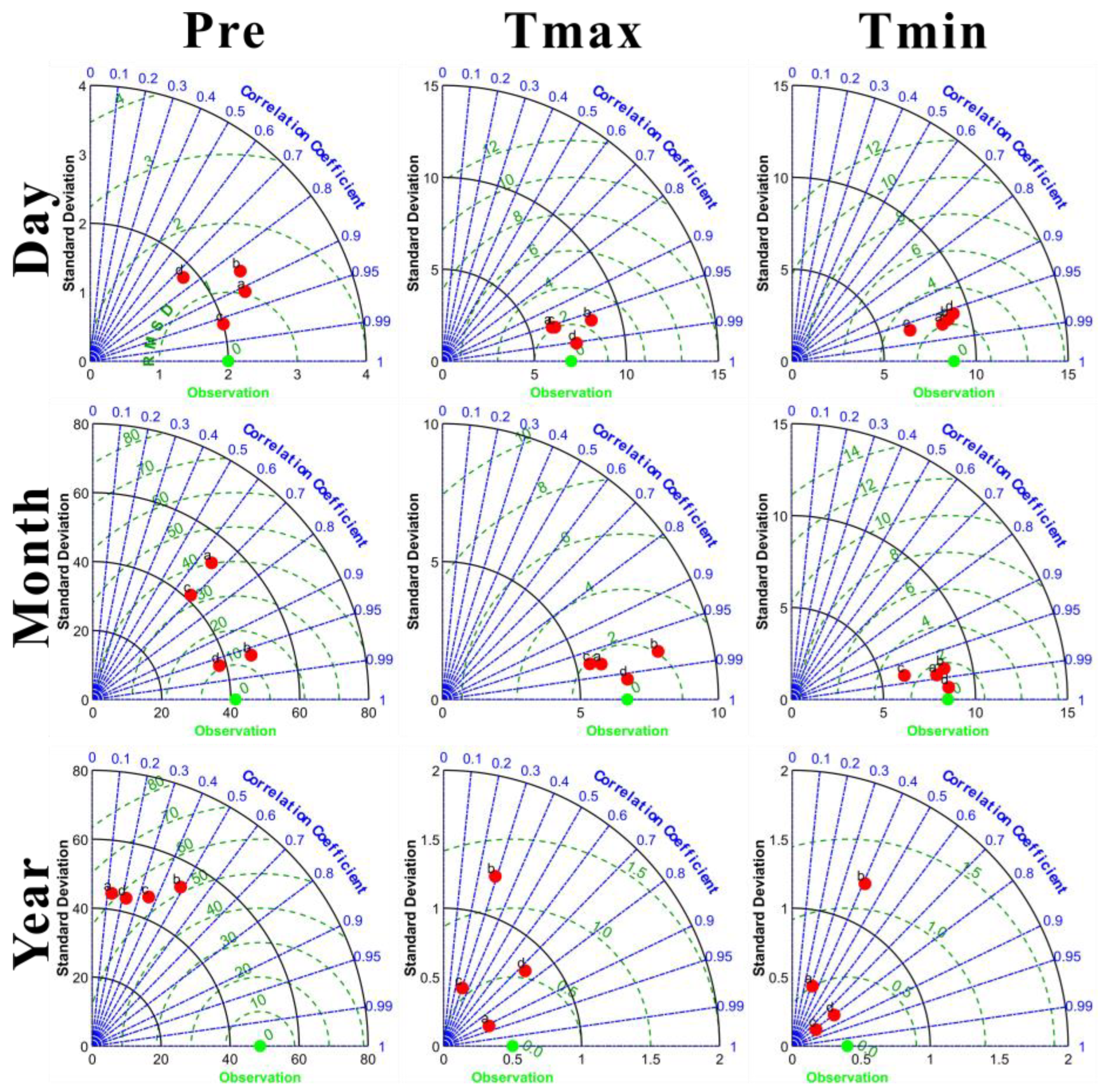
A quantitative understanding of how these reanalysis data compare to observations on different time scales can be found by looking at the correlation coefficient (i.e, CC), centered root mean square difference (i.e., RMSD), and standard deviation (i.e., STD). This can be summarized by a drawing of the Taylor diagram Figure 2. At the daily scale, CMFD performed best, followed by ERA5 and CFSR, while CMADS underperformed in terms of daily precipitation. For example, CMFD precipitation has the best correlation with observed precipitation (i.e., a correlation over 0.95) and its RMSD is also the smallest in the four reanalysis datasets used for evaluation (i.e., RMSD less than 1 mm/day), showing that CMFD is in excellent agreement with observed data, although the STD of CMFD is not the smallest. The correlation between ERA5 and CFSR with observations, although not as high as CMFD, is also satisfactory (i.e., the correlation also reaches 0.85–0.91), whereas the correlation between CMADS and observations is only 0.74, showing that ERA5 and CFSR are also representative of the precipitation characteristics of the SYYR region to some extent. Additionally, the standard deviation of CMFD is 2.01 mm/day, which is only 0.01 mm/day different from the standard deviation of 2.00 mm/day for the observations, showing that CMFD captures the variability of precipitation in the SYYR region well. Standard deviations greater than 2.00 mm/day for ERA5 and CFSR indicate a slight tendency to overestimate estimated precipitation, while CMADS tends to underestimate (i.e., standard deviation of 1.81 mm/day).
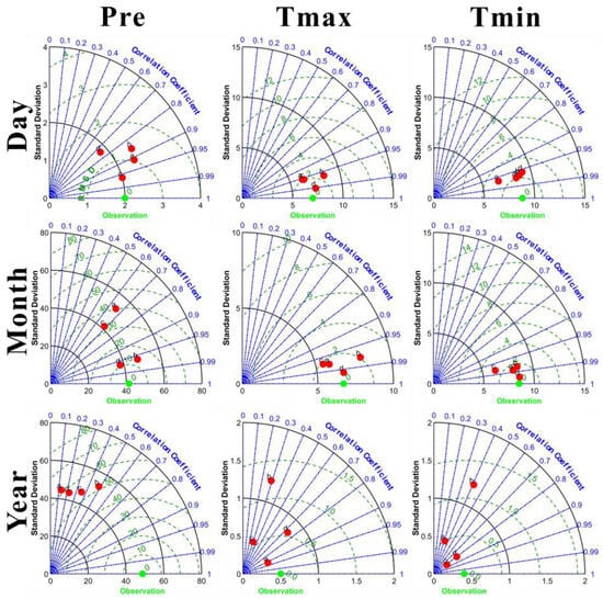
Figure 2.
Taylor plots of reanalysis datasets and observations on precipitation, maximum temperature, and minimum temperature for different time scales (daily/monthly/yearly) for 2008–2018. (a-ERA5, b-CFSR, c-CMFD, d-CMADS).
Meanwhile, CMFD has the highest POD and CSI and the smallest FAR in the four reanalysis datasets according to the performance diagrams in Figure 3, showing that CMFD performs well in the precipitation detection capability assessment. The four reanalysis products show similar performance, in most cases second only to CMFD, suggesting a robust occurrence detection mechanism. On the monthly scale, the performance of CMADS and CFSR is satisfactory (i.e., both correlation coefficients are greater than 0.95), while CMFD and ERA5 are not as good as at the daily scale (i.e., both correlation coefficients are less than 0.7). At the interannual scale, the four reanalysis datasets performed poorly, not only with correlation coefficients lower than 0.5, but also standard deviations and root mean square errors greater than 40 mm/year.
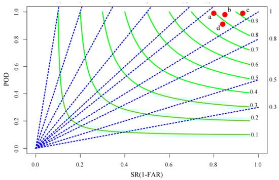
Figure 3.
Daily scale performance diagrams for the years 2008 to 2018 feature bias scores indicated by blue lines and the Comprehensive Similarity Index (CSI) represented by green lines (a-ERA5, b-CFSR, c-CMFD, d-CMADS).
3.1.2. Evaluation of the Temperature of Reanalysis Datasets by Time Scale
At the daily scale, the four reanalysis datasets performed satisfactorily in terms of maximum and minimum temperature, with the best being CMADS, followed by CMFD, and finally ERA5 and CFSR; all had correlation coefficients greater than 0.95. At the same time, the STD and RMSD of the four reanalysis datasets are relatively close and not significantly different to the observed data and show a cumulative state in the Taylor diagram, showing that the reanalysis dataset has high accuracy in temperature estimation. At the monthly scale, the four reanalysis datasets performed similarly to the daily scale at the monthly scale, with all showing satisfactory accuracy in temperature estimation, for both maximum and minimum temperatures. On the interannual scale, the four reanalysis data vary considerably in the accuracy of the temperature estimates, and the accuracy varies considerably between maximum and minimum temperatures. For example, among the datasets considered, ERA5 exhibits superior accuracy in capturing the mean annual maximum temperature (i.e., the correlation coefficient of 0.92), while the accuracy is very low in terms of mean annual minimum temperature (i.e., the correlation coefficient of only 0.32). The other three reanalysis datasets are similar to ERA5, which may be caused by the lower number of samples used for assessment at the annual scale.
3.1.3. Spatial Annual Averages: Reanalysis Datasets vs. OBS Data
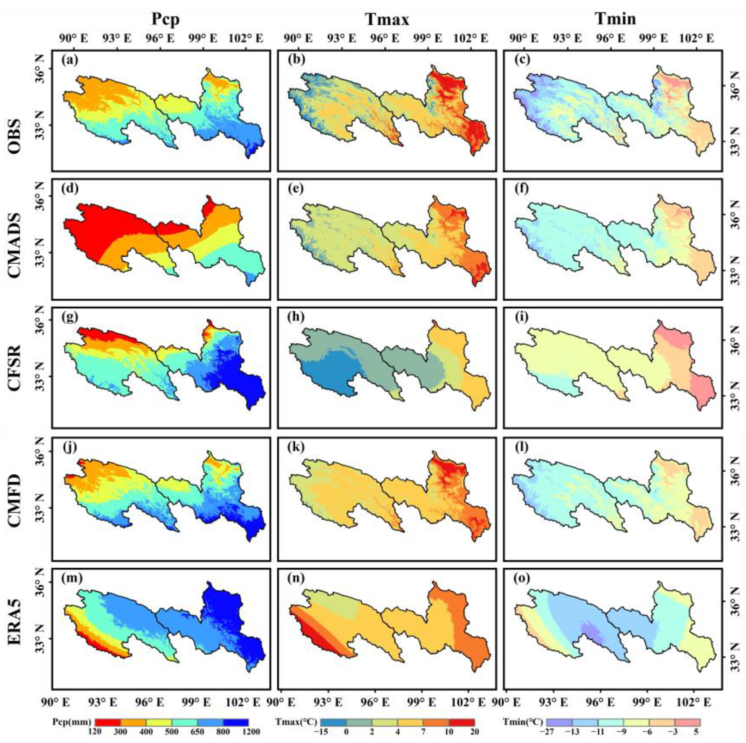
In order to spatially compare the differences between reanalysis datasets and OBS data, this study employs the ANUSPLIN interpolation methodology to interpolate annual mean precipitation as well as maximum and minimum temperatures within the SYYR region (Figure 4).

Figure 4.
Spatial distribution of reanalysis datasets and observed data. Subfigures in the first, second, and third columns illustrate the spatial distributions of annual average precipitation, maximum temperature, and minimum temperature, respectively ((a): OBS-Pcp, (b): OBS-Tmax, (c): OBS-Tmin, (d): CMADS-Pcp, (e): CMADS-Tmax, (f): CMADS-Tmin, (g): CFSR-Pcp, (h): CFSR-max, (i): CFSR-Tmin, (j): CMFD-Pcp, (k): CMFD-Tmax, (l): CMFD-Tmin, (m): ERA5-Pcp, (n): ERA5-Tamx, (o): ERA5-Tmin).
From Figure 4a, it was found that precipitation presents a decrease from southeast to northwest in the SYYR region. Due to the topographic obstruction and airflow uplift, water vapor from the ocean decreases in the process of moving from southeast to northwest, resulting in abundant precipitation in the southeastern part of the SYYR region, with annual precipitation ranging from 800 to 1200 mm, while precipitation is scarce in the northwest, with annual precipitation less than 300 mm. By comparing Figure 4a,d,g,j,m, it can be discerned that the annual precipitation across CMADS, CFSR, CMFD, ERA5, and observational (OBS) data in the SYYR region consistently displays a geographical pattern marked by higher values in the southeast and lower values in the northwest. In particular, the CMFD data are in excellent agreement with the spatial distribution of the observations. Furthermore, it is apparent that CMADS tends to exhibit a systematic underestimation of annual precipitation within the SYYR region, while both CFSR and ERA5 demonstrate a tendency toward overestimation. This observation aligns with the outcomes derived from the quantitative analysis presented in the preceding section.
From Figure 4b,c, the investigation reveals a discernible east-to-west decline in both the annual mean maximum and minimum temperatures across the SYYR region. This temperature variation is attributed to the elevation gradient, particularly evident in the transition from the relatively lower-elevation eastern Yellow River source area to the higher-elevation Yangtze River source area in the west. The temperature reduction is compounded by the latitudinal influence, contributing to relatively elevated temperatures in the southeastern corner of the Yangtze River source region. This phenomenon indicates that the influence of elevation gradient on the temperature in the SYYR region is greater than that of latitude. By comparing Figure 4b,e,h,k,n, a consensus is evident in the spatial distribution of the annual mean maximum temperature across CMADS, CFSR, CDMFD, and observational (OBS) data within the SYYR region. This commonality manifests as a geographical pattern characterized by higher values in the east and lower values in the west. However, ERA5 performed poorly and there was a significant overestimation of temperatures in the southwestern Yangtze River source. The spatial patterns observed in Figure 4c,f,i,l,o indicate a general coherence between the spatial distribution of the mean annual minimum temperature and that of the mean annual maximum temperature.
3.2. Hydrological Aspect
3.2.1. Calibration and Sensitivity Analysis of Parameters
The calibration of the SWAT model is executed by employing the Sequential Uncertainty Fitting Algorithm (SUFI-2) within the Uncertainty Procedure (SWAT-CUP). This method offers a versatile algorithm for the calibration of SWAT models characterized by a substantial number of input parameters [35]. The process of calibrating the SWAT model involved the application of global sensitivity analysis within SWAT-CUP, leading to the identification and selection of a total of 10 parameters for calibration. Table 4 lists the global sensitivity ranking of model parameters and their best-fit values for runoff simulations in the SYYR region. Across all simulations, the year 2008 was designated as the warm-up phase for model simulations, while the interval spanning 2009 to 2014 served as the model calibration period. Subsequently, the validation phase encompassed the years 2015 to 2018. Calibration and validation procedures were conducted at both the daily and monthly temporal scales.
Table 4.
Initial and optimized parameter values for the runoff simulation.
3.2.2. Flow Simulation in the SYYR
To mitigate uncertainties in the hydrological model, parameter uniformity is imperative among the various components of the hydrological model. Therefore, we first rigorously process the data based on observations, then adjust the reference to obtain the best parameters for input into SWAT, with the best parameters held constant, and then input different meteorological forcing data for simulation, so that the resulting hydrological processes are comparable.
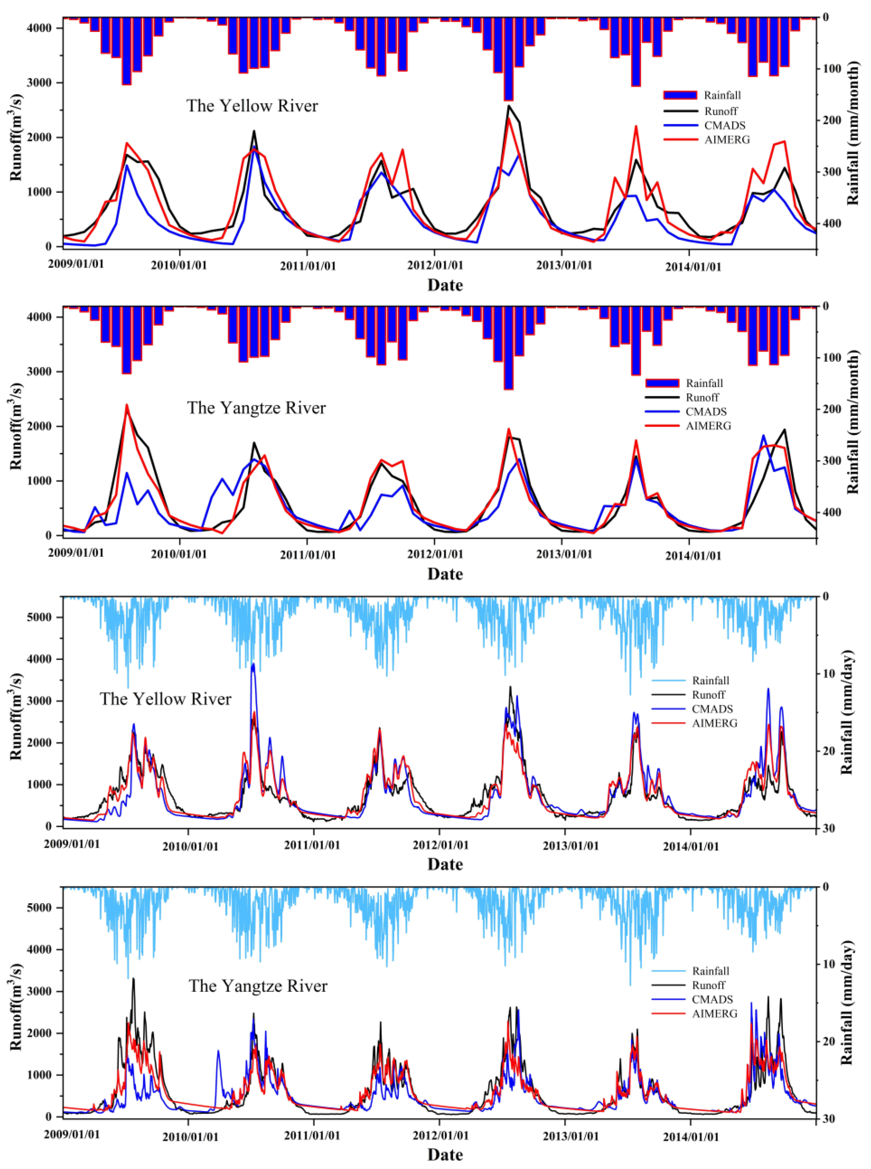
Upon calibration of parameters using observational data, diverse runoff simulations were generated by executing the SWAT model with varied meteorological datasets. Figure 5 presents the daily and monthly runoff simulations for the two hydrological stations, while Table 5 details the corresponding performance indicators. Comparative analysis of the runoff simulations using distinct input data reveals the superior performance of OBS-driven simulations, with CMFD demonstrating the closest resemblance, followed by ERA5 and CFSR. Conversely, CMADS exhibits comparatively inferior performance.
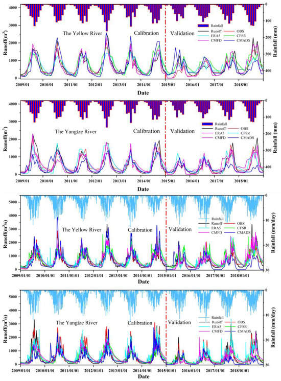
Figure 5.
Observed runoff and SWAT model simulations at hydrological stations, spanning the calibration period (2009–2014) and the validation period (2015–2018).
Table 5.
Performance metrics for daily and monthly runoff simulation.
In summary, the precision of runoff simulations generated by SWAT models generally exhibits a higher degree of accuracy at the monthly scale compared to the daily scale. Additionally, most reanalysis datasets adequately fulfill the data requirements for runoff simulations, with the notable exception of CMADS, which demonstrates suboptimal performance during the validation period. When coupled with the assessment outcomes of reanalysis data in Section 3.1, a notable correspondence emerges between the runoff simulation results and the evaluation of daily scale precipitation. Specifically, a one-to-one relationship is observed between the accuracy of runoff simulation and the precision of daily scale precipitation. It can be inferred that the accuracy of runoff simulation is heavily contingent upon the accuracy of daily scale precipitation within reanalysis datasets. This observation underscores the tendency in related research to primarily focus on the assessment of precipitation within reanalysis or satellite datasets. On the other hand, we note that there are differences in the accuracy of the reanalysis data for runoff simulations in the two basins. For example, although CMADS is less accurate in estimating daily precipitation, its simulation accuracy for monthly runoff in the Yellow River source area is better than that of CFSR and ERA5, while it performs poorly in the Yangtze River source area, most likely due to the spatial differences in the accuracy of the reanalysis data.
As can be seen from Figure 5, whether within the Yellow River or Yangtze River basin, the annual peak flow predominantly occurs during the period from May to September. Notably, during the calibration period (2009–2014), the highest daily average flow reached 3350.00 m3/s at the source of the Yellow River on 24 July 2012, and 3320.00 m3/s at the source of the Yangtze River on 24 July 2009. Employing the 95% quantile [36] of runoff values for the study period as the extreme runoff threshold (as illustrated in Figure 6), it was observed that, in most instances, both reanalysis datasets and observed data tend to underestimate peak flows during runoff simulations at the sources of both the Yellow River and the Yangtze. This discrepancy may arise from the SWAT model’s limitation in accurately representing the glacier and soil thawing processes in the SYYR region during the thaw period. Additionally, it fails to seamlessly integrate glacier meltwater and thawed soil water into the simulated runoff outcomes.
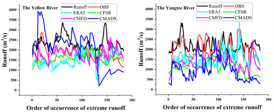
Figure 6.
Comparison of observed extreme runoff at >95% quantile with simulated runoff from SWAT.
4. Discussion
4.1. Uncertainty Analysis of Reanalysis Data
In general, the reanalysis data have good applicability in China and can obtain a relatively accurate runoff simulation by running the SWAT model. However, the study area in this paper is located on the Tibetan Plateau, which has a unique plateau climate with climatic differences from other regions in China [14]. Moreover, the spatial and temporal resolution, as well as the quality of the components, will exhibit variations across diverse reanalysis datasets, contingent upon factors such as the origin of the observed data, the forecast model/land surface model [37], the assimilation method [38], and other contributing parameters [39]. These factors could contribute to notable disparities in the precision and suitability of the four reanalysis datasets within the SYYR region.
The findings of this study indicate that, within the SYYR region, CMFD exhibits the highest level of applicability, succeeded by ERA5 and CFSR, whereas CMADS demonstrates suboptimal results in runoff simulation due to its diminished performance in daily scale precipitation. Notably, CMFD and CMADS assimilate ground-based observations with multiple gridded datasets sourced from remote sensing and reanalysis [40]. Given the constraints associated with ground observations, particularly in regions of elevated terrain complexity, direct interpolation of variable values may yield greater errors compared to the interpolation of differences or ratios between station data and background data [41]. CMFD employed distinct data generation algorithms tailored for various variables [42]. Notably, the precipitation generation algorithm employed a positive bias suppression method, wherein precipitation interpolation was conducted separately for sub-daily and -monthly scales. Subsequently, the sub-daily interpolated values were adjusted based on the corresponding monthly interpolated values [43], which greatly improves data accuracy. ERA5 is a comprehensive reanalysis dataset which assimilates as many observations as possible in the upper atmosphere and near the surface [44,45]. In regions with limited observational coverage, ERA5 employs a weather forecasting model to furnish spatially and temporally continuous data. This dataset is generated through the utilization of 4D-Var data assimilation and model forecasts within the CY41R2 version of the ECMWF Integrated Forecast System (IFS) [46]. ERA5 integrates available weather observations and complements them with a weather forecasting model to yield continuous data with spatial and temporal coverage. The resultant dataset, resembling a weather forecast, inherently carries a degree of uncertainty. Conversely, CFSR stands as a comprehensive, long-term reanalysis dataset crafted by the U.S. National Centers for Environmental Prediction. It encompasses both the coupled land–atmosphere–ocean model and the Global Land Data Assimilation System (GLDAS) [47]. Although its data quality has improved after the upgrade transition from CFSv1 to CFSv2, the resulting data necessarily contain some uncertainty as they seem not to assimilate ground-based observations [48], but to produce data in a forecast manner. CMADS was constructed through the application of diverse techniques, including data loop nesting, resampling, and bilinear interpolation. This process was rooted in the utilization of field elements derived from the China Meteorological Administration Land Data Assimilation System (CLDAS) as the foundational dataset [49]. This may be one of the reasons for the lower accuracy of CMADS in terms of daily scale precipitation, which is also consistent with the findings of Zhang et al. [49] and Dao et al. [50]. Nevertheless, CMADS merits acknowledgment for its commendable precision in temperature estimates, yielding satisfactory outcomes across the annual, monthly, and daily temporal scales. Consequently, an evaluation of climate data source accuracy becomes imperative when employing reanalysis datasets at a regional scale, particularly in areas with limited meteorological station coverage.
4.2. Optimization of the CMADS Dataset
The SYYR region is one of China’s important nature reserves, where human activities have relatively little impact on the natural environment [51]. Moreover, the predominant sources of water supply to rivers in the region consist primarily of natural precipitation and glacial meltwater. Consequently, the regional runoff is primarily shaped by natural factors [5,52]. In this investigation, an initial exploration of the influence of precipitation, temperature, and solar radiation on runoff in the SYYR region was conducted at a monthly scale using path analysis. This analysis was based on a synthesis of regional characteristics and the data essential for runoff simulation with the SWAT model, as illustrated in Figure 7. The findings reveal that temperature exerts the most substantial direct impact on runoff in the SYYR region, followed by solar radiation, with precipitation exhibiting the least direct influence. Li et al. [53] argued that with global warming and increasing temperatures, on the one hand, the depth of permafrost freezing decreases, glacial snowmelt increases, and evaporation increases in the basin, leading to a greater effect of temperature on runoff. On the other hand, the rise in temperature alters the characteristics of the basin’s underlying surface, leading to an augmentation in soil layer thickness. This, in turn, escalates the proportion of precipitation contributing to groundwater recharge while diminishing direct surface runoff. Consequently, the impact of temperature on runoff in the SYYR region becomes more pronounced.
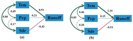
Figure 7.
Path analysis of runoff changes in the SYYR region, (a) the Yellow River; (b) the Yangtze River. Green color indicates a positive effect, red color indicates a negative effect, and the thickness of the line represents the magnitude of the effect.
From the results of this paper, it is clear that CMADS does not perform well in precipitation, but it presents good results in temperature simulation. Therefore, the author advocates for the utilization of meteorological data products demonstrating superior precision in precipitation estimation or corresponding satellite data products to address the deficiencies observed in CMADS regarding precipitation. Notably, prior studies have consistently demonstrated a strong correlation between the daily precipitation data from IMERG and surface precipitation across China [54,55,56].
In this study, the selection is made for AIMERG, which is acquired through the implementation of an innovative spatiotemporal correction algorithm. Additionally, the integration of a high-quality ground-based observation product, APHRODITE, is employed to rectify the GPM IMERG satellite precipitation product [23]. The AIMERG precipitation dataset effectively integrates the respective merits of satellite estimation and ground-based observations, exhibiting superior performance in systematic bias and random errors across diverse spatial and temporal scales in China, thereby furnishing a more dependable foundational dataset for scientific research and applications in related fields across Asia [57,58]. Employing Python and Matlab tools, precipitation data from AIMERG was extracted and substituted for corresponding points in CMADS, ensuring the continuity of other input data. Subsequently, the SWAT model underwent recalibration to simulate runoff in the SYYR region, with the stipulation that the remaining input data remained unaltered. The result shows (Table 6) that the CMADS data optimized with AIMERG are more suitable for runoff simulation in the SYYR area (Figure 8), especially in the Yangtze River source area, where the R2 and NSE for monthly scale runoff simulation increased from 0.55 and 0.54 to 0.86 and 0.86, respectively, and the R2 and NSE for monthly scale runoff simulation increased from 0.53 and 0.50 to 0.82 and 0.79.
Table 6.
Evaluation Indicators for Daily and Monthly Runoff Simulation for CMADS and AIMERG + CMADS.
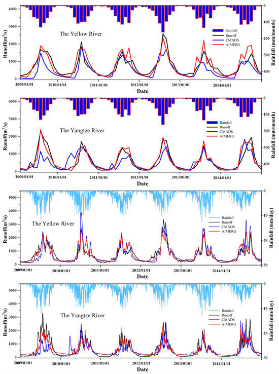
Figure 8.
Simulation results of observed monthly runoff and the AIMERG-optimized CMADS-driven SWAT model at hydrological stations during the calibration period (2009–2014).
The refinement of the CMADS dataset through the application of the substitution method has yielded a significant enhancement in its accuracy. This approach, characterized by its simplicity and accessibility, contrasts with the intricate methodologies employed by other researchers in optimizing and fusing reanalysis data. These methodologies encompass sophisticated techniques, including artificial neural networks [59], wavelet transform methods [60], genetic algorithms [61,62], and machine learning [63,64]. However, it is noteworthy that the efficacy of the aforementioned optimization is constrained to situations akin to CMADS, where certain metrics exhibit suboptimal performance relative to others.
4.3. Limitations
Within the confines of the SWAT model framework, notwithstanding the incorporation of parameters pertinent to snowmelt, it is imperative to acknowledge the model’s omission of pivotal freeze–thaw phenomena manifesting in soils and glaciers. This lacuna encompasses the nuanced influences exerted by seasonal permafrost, permafrost, and glacial melt on the hydrological process of runoff. Particularly noteworthy are investigations conducted by Wang et al. [65] and Xin et al. [66], which have astutely recognized the substantive repercussions of these processes on streamflow dynamics. And the depth of perennial permafrost on the Tibetan Plateau has decreased in recent years [67]. The concurrent presence of permafrost and seasonal permafrost introduces limitations on interfacial water fluxes encompassing the terrestrial surface, the cryosphere, and the unfrozen lithosphere beneath [68]. This constraint engenders a diminution in the soil surface’s infiltration capacity and the hydraulic conductivity of the soil, instigating alterations in surface hydrodynamics, subsurface groundwater transport, and subsequent disruptions to ecosystem functioning [69,70]. Conversely, the escalating influence of glacial meltwater on runoff dynamics within the SYYR region necessitates the development of an analogous algorithmic framework or a module dedicated to simulating soil and glacier freeze–thaw processes within the SWAT model. Previous endeavors, exemplified by Omani et al. [71] and Qi et al. [72], sought to devise methodologies incorporating soil temperature and glacier mass balance simulations. Nevertheless, extant accomplishments underscore discernible lacunae the envisioned objectives, thus underscoring the imperative for future research endeavors aimed at ameliorating these gaps.
Furthermore, the role of groundwater in runoff simulation within the SWAT model in alpine regions is of paramount importance. The substantial impact of groundwater on soil moisture dynamics, particularly in cooler climates, is undeniable, and its pivotal role in mitigating runoff constraints arising from soil freezing cannot be disregarded [70]. However, the somewhat simplified delineation of groundwater processes in the SWAT model may not comprehensively encapsulate the intricate interplay between groundwater dynamics and soil moisture dynamics [73]. The optimization of the groundwater–surface water linkage within the SWAT model can be achieved by incorporating a more nuanced depiction of interaction mechanisms between groundwater and surface water [74]. Furthermore, enhancing the parameterization process governing groundwater–surface water interaction within the model is imperative to elucidate groundwater dynamics with greater granularity in forthcoming research endeavors.
5. Conclusions
In this study, three meteorological elements, precipitation, and maximum and minimum temperature of the reanalysis datasets CMADS, CFSR, CMFD, and ERA5 were initially evaluated based on daily, monthly, and annual time scales by using 28 meteorological station observations from 2008 to 2018 in the SYYR region. And the five meteorological datasets (OBS, CMADS, CFSR, CMFD, and ERA5) were also applied to the SWAT model to compare the performance of each dataset in the simulation of runoff. Additionally, the CMADS dataset was also optimized using AIMERG satellite precipitation data based on the assessment results of meteorological elements and the hydroclimatic characteristics of the SYYR region, and satisfactory results were obtained. In summary, the principal findings of this study are outlined as follows:
- (1)
- On the daily scale, in terms of climate, CMFD performs best (i.e., correlation over 0.95 and RMSD less than 1 mm/day), followed by ERA5 and CFSR, while CMADS performs poorly in terms of daily precipitation (i.e., correlation only 0.74). The four reanalysis datasets performed well in terms of temperature at the daily and monthly scales (i.e., correlation over 0.95), but not satisfactorily at the annual scales.
- (2)
- In runoff simulations, SWAT has better simulation accuracy at the monthly scale than at the daily scale. The best runoff simulation was based on OBS data (with R2 > 0.80, NSE > 0.80 during the calibration period), and the closest to the OBS simulation results was CMFD, followed by ERA5 and CFSR, while CMADS was the worst performer.
- (3)
- Reanalysis data and the observed data in most cases underestimated the peak flows to varying degrees in the runoff simulations carried out, and failed to effectively capture the extreme runoff characteristics of the basin, both at the source of the Yellow River and the Yangtze.
- (4)
- After optimizing CMADS with the AIMERG precipitation dataset, the runoff simulation performance was greatly improved, with R2 and NSE increasing from 0.55 and 0.54 to 0.86 and 0.86 for the source of the Yangtze at the monthly scale and from 0.53 and 0.50 to 0.82 and 0.79 at the daily scale, respectively.
Ultimately, we posit that a meticulous evaluation of the precision inherent in reanalyzed data becomes imperative when employing such datasets at a regional scale, particularly in regions characterized by a paucity of weather station coverage. In the context of the SYYR region scrutinized within this study, it is undoubtable that the CMFD dataset and the refined iteration of CMADS stand out as the most apt choices.
Author Contributions
X.W. (Xiaofeng Wang): conceptualization, data curation, supervision, resources, writing—review and editing; J.Z.: conceptualization, methodology, software, data curation, investigation, validation, formal analysis, visualization, writing—original draft, writing—review and editing; J.M.: validation, writing—review and editing; P.L.: supervision, data curation, resources, writing—review and editing; X.F. (Xinxin Fu): data curation, supervision, writing—review and editing; X.F. (Xiaoming Feng): resources, project administration, funding acquisition; X.Z.: visualization, supervision, writing—review and editing; Z.J.: data curation, supervision, validation, writing—review and editing; X.W. (Xiaoxue Wang): validation, writing—review and editing; X.H.: visualization, formal analysis. All authors have read and agreed to the published version of the manuscript.
Funding
This research was funded by the Second Tibetan Plateau Scientific Expedition and Research Program Tibetan, grant number 2019QZKK0405, the Chinese Academy of Sciences, Strategic Pilot Science and Technology Project (Class A), grant number XDA2002040201, and the Fundamental Research Funds for the Central Universities, CHD, grant number 300102352201.
Data Availability Statement
The download addresses for all data can be obtained from Table 1 in the manuscript.
Conflicts of Interest
The authors declare no conflicts of interest.
References
- Wang, T.; Sun, B.; Wang, H. Interannual variations of monthly precipitation and associated mechanisms over the Three River Source region in China in winter months. Int. J. Climatol. 2021, 41, 2209–2225. [Google Scholar] [CrossRef]
- Jiang, C.; Zhang, L. Effect of ecological restoration and climate change on ecosystems: A case study in the Three-Rivers Headwater Region, China. Environ. Monit. Assess. 2016, 188, 382. [Google Scholar] [CrossRef] [PubMed]
- Liu, J.; Xu, X.; Shao, Q. Grassland degradation in the “Three-River Headwaters” region, Qinghai Province. J. Geogr. Sci. 2008, 18, 259–273. [Google Scholar] [CrossRef]
- Yang, K.; Wu, H.; Qin, J.; Lin, C.; Tang, W.; Chen, Y. Recent climate changes over the Tibetan Plateau and their impacts on energy and water cycle: A review. Glob. Planet. Chang. 2014, 112, 79–91. [Google Scholar] [CrossRef]
- Wang, Y.; Xie, X.; Shi, J.; Zhu, B. Ensemble runoff modeling driven by multi-source precipitation products over the Tibetan Plateau. Chin. Sci. Bull. 2021, 66, 4169–4186. [Google Scholar] [CrossRef]
- Ji, P.; Yuan, X. High-Resolution Land Surface Modeling of Hydrological Changes over the Sanjiangyuan Region in the Eastern Tibetan Plateau: 2. Impact of Climate and Land Cover Change. J. Adv. Model. Earth Syst. 2018, 10, 2829–2843. [Google Scholar] [CrossRef]
- Li, F.; Zhang, Y.; Xu, Z.; Liu, C.; Zhou, Y.; Liu, W. Runoff predictions in ungauged catchments in southeast Tibetan Plateau. J. Hydrol. 2014, 511, 28–38. [Google Scholar] [CrossRef]
- Sun, Y.; Bao, W.; Jiang, P.; Xu, Y.; He, C.; Chen, W.; Huang, L. Real-time updating of XAJ model by using Unscented Kalman Filter. J. Lake Sci. 2018, 30, 488–496. [Google Scholar]
- Dal Molin, M.; Schirmer, M.; Zappa, M.; Fenicia, F. Understanding dominant controls on streamflow spatial variability to set up a semi-distributed hydrological model: The case study of the Thur catchment. Hydrol. Earth Syst. Sci. 2020, 24, 1319–1345. [Google Scholar] [CrossRef]
- Liu, Y.; Zhou, Z.; Liu, J.; Wang, P.; Li, Y.; Zhu, Y.; Jiang, X.; Wang, K.; Wang, F. Distributed hydrological model of the Qinghai Tibet Plateau based on the hydrothermal coupling: II: Simulation of water cycle processes in the Niyang River basin considering glaciers and frozen soils? Adv. Water Sci. 2021, 32, 201–210. [Google Scholar]
- Goyal, M.K.; Panchariya, V.K.; Sharma, A.; Singh, V. Comparative Assessment of SWAT Model Performance in two Distinct Catchments under Various DEM Scenarios of Varying Resolution, Sources and Resampling Methods. Water Resour. Manag. 2018, 32, 805–825. [Google Scholar] [CrossRef]
- Grusson, Y.; Anctil, F.; Sauvage, S.; Sánchez Pérez, J. Testing the SWAT Model with Gridded Weather Data of Different Spatial Resolutions. Water 2017, 9, 54. [Google Scholar] [CrossRef]
- Eini, M.R.; Javadi, S.; Delavar, M.; Monteiro, J.A.F.; Darand, M. High accuracy of precipitation reanalyses resulted in good river discharge simulations in a semi-arid basin. Ecol. Eng. 2019, 131, 107–119. [Google Scholar] [CrossRef]
- You, Q.; Kang, S.; Li, J.; Chen, D.; Zhai, P.; Ji, Z. Several research frontiers of climate change over the Tibetan Plateau. J. Glaciol. 2021, 43, 885–901. [Google Scholar]
- Sun, Q.; Miao, C.; Duan, Q.; Ashouri, H.; Sorooshian, S.; Hsu, K.L. A Review of Global Precipitation Data Sets: Data Sources, Estimation, and Intercomparisons. Rev. Geophys. 2018, 56, 79–107. [Google Scholar] [CrossRef]
- Tan, M.L.; Gassman, P.W.; Liang, J.; Haywood, J.M. A review of alternative climate products for SWAT modelling: Sources, assessment and future directions. Sci. Total Environ. 2021, 795, 148915. [Google Scholar] [CrossRef] [PubMed]
- Bosilovich, M.G.; Chen, J.; Robertson, F.R.; Adler, R.F. Evaluation of Global Precipitation in Reanalyses. J. Appl. Meteorol. Clim. 2008, 47, 2279–2299. [Google Scholar] [CrossRef]
- Ndhlovu, G.Z.; Woyessa, Y.E. Use of gridded climate data for hydrological modelling in the Zambezi River Basin, Southern Africa. J. Hydrol. 2021, 602, 126749. [Google Scholar] [CrossRef]
- Qi, D.; Zhang, S.; Li, Y. Research Progress on Variations of the Climate and Water Resourcesin the Source Region of the Yangtze River. Plateau Mt. Meteorol. Res. 2013, 33, 89–96. [Google Scholar]
- Jin, J.; Wang, G.; Zhang, J.; Yang, Q.; Liu, C.; Liu, Y.; Bao, Z.; He, R. Impacts of climate change on hydrology in the Yellow River source region, China. J. Water Clim. Chang. 2020, 11, 916–930. [Google Scholar] [CrossRef]
- Meng, X.; Wang, H.; Chen, J. Profound Impacts of the China Meteorological Assimilation Driving Datasets for the SWAT Model (CMADS). Water 2019, 11, 832. [Google Scholar] [CrossRef]
- Fuka, D.R.; Walter, M.T.; MacAlister, C.; Degaetano, A.T.; Steenhuis, T.S.; Easton, Z.M. Using the Climate Forecast System Reanalysis as weather input data for watershed models. Hydrol. Process. 2014, 28, 5613–5623. [Google Scholar] [CrossRef]
- Ma, Z.; Xu, J.; Zhu, S.; Yang, J.; Tang, G.; Yang, Y.; Shi, Z.; Hong, Y. AIMERG: A new Asian precipitation dataset (0.1 degrees/half-hourly, 2000–2015) by calibrating the GPM-era IMERG at a daily scale using APHRODITE. Earth Syst. Sci. Data 2020, 12, 1525–1544. [Google Scholar] [CrossRef]
- Havrylenko, S.B.; Bodoque, J.M.; Srinivasan, R.; Zucarelli, G.V.; Mercuri, P. Assessment of the soil water content in the Pampas region using SWAT. Catena 2016, 137, 298–309. [Google Scholar] [CrossRef]
- Awan, U.K.; Ismaeel, A. A new technique to map groundwater recharge in irrigated areas using a SWAT model under changing climate. J. Hydrol. 2014, 519, 1368–1382. [Google Scholar] [CrossRef]
- Kondo, T.; Sakai, N.; Yazawa, T.; Shimizu, Y. Verifying the applicability of SWAT to simulate fecal contamination for watershed management of Selangor River, Malaysia. Sci. Total Environ. 2021, 774, 145075. [Google Scholar] [CrossRef]
- Lin, F.; Chen, X.; Yao, W.; Fang, Y.; Deng, H.; Wu, J.; Lin, B. Multi-time scale analysis of water conservation in a discontinuous forest watershed based on SWAT model. Acta Geogr. Sin. 2020, 75, 1065–1078. [Google Scholar]
- Pombo, S.; de Oliveira, R.P. Evaluation of extreme precipitation estimates from TRMM in Angola. J. Hydrol. 2015, 523, 663–679. [Google Scholar] [CrossRef]
- Tan, M.; Duan, Z. Assessment of GPM and TRMM Precipitation Products over Singapore. Remote Sens. 2017, 9, 720. [Google Scholar] [CrossRef]
- Xu, Z.; Han, Y. Short communication comments on ‘DISO: A rethink of Taylor diagram’. Int. J. Climatol. 2020, 40, 2506–2510. [Google Scholar] [CrossRef]
- Pomee, M.S.; Hertig, E. Precipitation projections over the Indus River Basin of Pakistan for the 21st century using a statistical downscaling framework. Int. J. Climatol. 2022, 42, 289–314. [Google Scholar] [CrossRef]
- Randriatsara, H.H.R.H.; Hu, Z.; Xu, X.; Ayugi, B.; Sian, K.T.C.L.; Mumo, R.; Ongoma, V. Evaluation of gridded precipitation datasets over Madagascar. Int. J. Climatol. 2022, 42, 7028–7046. [Google Scholar] [CrossRef]
- Tang, G.; Clark, M.P.; Papalexiou, S.M.; Ma, Z.; Hong, Y. Have satellite precipitation products improved over last two decades? A comprehensive comparison of GPM IMERG with nine satellite and reanalysis datasets. Remote Sens. Environ. 2020, 240, 111697. [Google Scholar] [CrossRef]
- Moriasi, D.N.; Gitau, M.W.; Pai, N.; Daggupati, P. Hydrologic and Water Quality Models: Performance Measures and Evaluation Criteria. Trans. ASABE 2015, 58, 1763–1785. [Google Scholar]
- Abbaspour, K.C.; Rouholahnejad, E.; Vaghefi, S.; Srinivasan, R.; Yang, H.; Kløve, B. A continental-scale hydrology and water quality model for Europe: Calibration and uncertainty of a high-resolution large-scale SWAT model. J. Hydrol. 2015, 524, 733–752. [Google Scholar] [CrossRef]
- Chen, X.; Chen, W.; Huang, G. Future Climatic Projections and Hydrological Responses in the Upper Beijiang River Basin of South China Using Bias-Corrected RegCM 4.6 Data. J. Geophys. Res. Atmos. 2021, 126, e2021JD034550. [Google Scholar] [CrossRef]
- Mararakanye, N.; Le Roux, J.J.; Franke, A.C. Using satellite-based weather data as input to SWAT in a data poor catchment. Phys. Chem. Earth Parts A/B/C 2020, 117, 102871. [Google Scholar] [CrossRef]
- Dhanesh, Y.; Bindhu, V.M.; Senent-Aparicio, J.; Brighenti, T.M.; Ayana, E.; Smitha, P.S.; Fei, C.; Srinivasan, R. A Comparative Evaluation of the Performance of CHIRPS and CFSR Data for Different Climate Zones Using the SWAT Model. Remote Sens. 2020, 12, 3088. [Google Scholar] [CrossRef]
- Baatz, R.; Hendricks Franssen, H.J.; Euskirchen, E.; Sihi, D.; Dietze, M.; Ciavatta, S.; Fennel, K.; Beck, H.; De Lannoy, G.; Pauwels, V.R.N.; et al. Reanalysis in Earth System Science: Toward Terrestrial Ecosystem Reanalysis. Rev. Geophys. 2021, 59, e2020RG000715. [Google Scholar] [CrossRef]
- Zhang, H.; Yang, T.; Bah, A.; Luo, Z.; Chen, G.; Xie, Y. Analysis of the Applicability of Multisource Meteorological Precipitation Data in the Yunnan-Kweichow-Plateau Region at Multiple Scales. Atmosphere 2023, 14, 701. [Google Scholar] [CrossRef]
- Pepin, N.C.; Arnone, E.; Gobiet, A.; Haslinger, K.; Kotlarski, S.; Notarnicola, C.; Palazzi, E.; Seibert, P.; Serafin, S.; Schöner, W.; et al. Climate Changes and Their Elevational Patterns in the Mountains of the World. Rev. Geophys. 2022, 60, e2020RG000730. [Google Scholar] [CrossRef]
- Hao, Y.; Baik, J.; Choi, M. Combining generalized complementary relationship models with the Bayesian Model Averaging method to estimate actual evapotranspiration over China. Agric. For. Meteorol. 2019, 279, 107759. [Google Scholar] [CrossRef]
- He, J.; Yang, K.; Tang, W.; Lu, H.; Qin, J.; Chen, Y.; Li, X. The first high-resolution meteorological forcing dataset for land process studies over China. Sci. Data 2020, 7, 25. [Google Scholar] [CrossRef]
- Jiang, C.; Xu, T.; Wang, S.; Nie, W.; Sun, Z. Evaluation of Zenith Tropospheric Delay Derived from ERA5 Data over China Using GNSS Observations. Remote Sens. 2020, 12, 663. [Google Scholar] [CrossRef]
- Li, H.; Chen, R.; Han, C.; Yang, Y. Evaluation of the Spatial and Temporal Variations of Condensation and Desublimation over the Qinghai–Tibet Plateau Based on Penman Model Using Hourly ERA5-Land and ERA5 Reanalysis Datasets. Remote Sens. 2022, 14, 5815. [Google Scholar] [CrossRef]
- Hersbach, H.; Bell, B.; Berrisford, P.; Hirahara, S.; Horányi, A.; Muñoz Sabater, J.; Nicolas, J.; Peubey, C.; Radu, R.; Schepers, D.; et al. The ERA5 global reanalysis. Q. J. R. Meteorol. Soc. 2020, 146, 1999–2049. [Google Scholar] [CrossRef]
- Saha, S.; Moorthi, S.; Wu, X.; Wang, J.; Nadiga, S.; Tripp, P.; Behringer, D.; Hou, Y.; Chuang, H.; Iredell, M.; et al. The NCEP Climate Forecast System Version 2. J. Clim. 2014, 27, 2185–2208. [Google Scholar] [CrossRef]
- Ghimire, U.; Akhtar, T.; Shrestha, N.K.; Paul, P.K.; Schürz, C.; Srinivasan, R.; Daggupati, P. A Long-term Global Comparison of IMERG and CFSR with Surface Precipitation Stations. Water Resour. Manag. 2022, 36, 5695–5709. [Google Scholar] [CrossRef]
- Zhang, L.; Meng, X.; Wang, H.; Yang, M.; Cai, S. Investigate the Applicability of CMADS and CFSR Reanalysis in Northeast China. Water 2020, 12, 996. [Google Scholar] [CrossRef]
- Dao, D.M.; Lu, J.; Chen, X.; Kantoush, S.A.; Binh, D.V.; Phan, P.; Tung, N.X. Predicting Tropical Monsoon Hydrology Using CFSR and CMADS Data over the Cau River Basin in Vietnam. Water 2021, 13, 1314. [Google Scholar] [CrossRef]
- Ma, B.; Zeng, W.; Xie, Y.; Wang, Z.; Hu, G.; Li, Q.; Cao, R.; Zhuo, Y.; Zhang, T. Boundary delineation and grading functional zoning of Sanjiangyuan National Park based on biodiversity importance evaluations. Sci. Total Environ. 2022, 825, 154068. [Google Scholar] [CrossRef] [PubMed]
- Wang, L.; Yao, T.; Chai, C.; Cuo, L.; Su, F.; Zhang, F.; Yao, Z.; Zhang, Y.; Li, X.; Qi, J.; et al. Monitoring and Quantifying Total River Runoff from the Third Pole. Bull. Am. Meteorol. Soc. 2020, 5, E948–E965. [Google Scholar] [CrossRef]
- Li, W.Z.; Liu, W.; Zhang, T.F. The contribution rate of climate and human activities on runoff change in the source regions of Yellow River. J. Glaciol. Geocryol. 2018, 40, 958–992. [Google Scholar]
- Guo, H.; Chen, S.; Bao, A.; Behrangi, A.; Hong, Y.; Ndayisaba, F.; Hu, J.; Stepanian, P.M. Early assessment of Integrated Multi-satellite Retrievals for Global Precipitation Measurement over China. Atmos. Res. 2016, 176–177, 121–133. [Google Scholar] [CrossRef]
- Tang, G.; Ma, Y.; Long, D.; Zhong, L.; Hong, Y. Evaluation of GPM Day-1 IMERG and TMPA Version-7 legacy products over Mainland China at multiple spatiotemporal scales. J. Hydrol. 2016, 533, 152–167. [Google Scholar] [CrossRef]
- Tang, G.; Zeng, Z.; Long, D.; Guo, X.; Yong, B.; Zhang, W.; Hong, Y. Statistical and Hydrological Comparisons between TRMM and GPM Level-3 Products over a Midlatitude Basin: Is Day-1 IMERG a Good Successor for TMPA 3B42V7? J. Hydrometeorol. 2016, 17, 121–137. [Google Scholar] [CrossRef]
- Zhang, L.; Gao, L.; Chen, J.; Zhao, L.; Zhao, J.; Qiao, Y.; Shi, J. Comprehensive evaluation of mainstream gridded precipitation datasets in the cold season across the Tibetan Plateau. J. Hydrol. Reg. Stud. 2022, 43, 101186. [Google Scholar] [CrossRef]
- Sengupta, A.; Vissa, N.K.; Roy, I. Assessing the performance of satellite derived and reanalyses data in capturing seasonal changes in extreme precipitation scaling rates over the Indian subcontinent. Atmos. Res. 2023, 288, 106741. [Google Scholar] [CrossRef]
- Peña-Arancibia, J.L.; van Dijk, A.I.J.M.; Renzullo, L.J.; Mulligan, M. Evaluation of Precipitation Estimation Accuracy in Reanalyses, Satellite Products, and an Ensemble Method for Regions in Australia and South and East Asia. J. Hydrometeorol. 2013, 14, 1323–1333. [Google Scholar] [CrossRef]
- Hu, Z.; Chai, L.; Crow, W.T.; Liu, S.; Zhu, Z.; Zhou, J.; Qu, Y.; Liu, J.; Yang, S.; Lu, Z. Applying a Wavelet Transform Technique to Optimize General Fitting Models for SM Analysis: A Case Study in Downscaling over the Qinghai–Tibet Plateau. Remote Sens. 2022, 14, 3063. [Google Scholar] [CrossRef]
- Zerenner, T.; Venema, V.; Friederichs, P.; Simmer, C. Multi-objective downscaling of precipitation time series by genetic programming. Int. J. Climatol. 2021, 41, 6162–6182. [Google Scholar] [CrossRef]
- Horton, P.; Jaboyedoff, M.; Obled, C. Using genetic algorithms to optimize the analogue method for precipitation prediction in the Swiss Alps. J. Hydrol. 2018, 556, 1220–1231. [Google Scholar] [CrossRef]
- Islam, K.I.; Elias, E.; Carroll, K.C.; Brown, C. Exploring Random Forest Machine Learning and Remote Sensing Data for Streamflow Prediction: An Alternative Approach to a Process-Based Hydrologic Modeling in a Snowmelt-Driven Watershed. Remote Sens. 2023, 15, 3999. [Google Scholar] [CrossRef]
- Fernandez-Palomino, C.A.; Hattermann, F.F.; Krysanova, V.; Lobanova, A.; Vega-Jácome, F.; Lavado, W.; Santini, W.; Aybar, C.; Bronstert, A. A novel high-resolution gridded precipitation dataset for Peruvian and Ecuadorian watersheds—Development and hydrological evaluation. J. Hydrometeorol. 2022, 23, 309–336. [Google Scholar]
- Wang, T.; Yang, H.; Yang, D.; Qin, Y.; Wang, Y. Quantifying the streamflow response to frozen ground degradation in the source region of the Yellow River within the Budyko framework. J. Hydrol. 2018, 558, 301–313. [Google Scholar] [CrossRef]
- Xin, J.; Sun, X.; Liu, L.; Li, H.; Liu, X.; Li, X.; Cheng, L.; Xu, Z. Quantifying the contribution of climate and underlying surface changes to alpine runoff alterations associated with glacier melting. Hydrol. Process. 2021, 35, e14069. [Google Scholar] [CrossRef]
- Qin, Y.; Yang, D.; Gao, B.; Wang, T.; Chen, J.; Chen, Y.; Wang, Y.; Zheng, G. Impacts of climate warming on the frozen ground and eco-hydrology in the Yellow River source region, China. Sci. Total Environ. 2017, 605–606, 830–841. [Google Scholar] [CrossRef] [PubMed]
- Cherkauer, K.A.; Lettenmaier, D.P. Hydrologic effects of frozen soils in the upper Mississippi River basin. J. Geophys. Res. 1999, 104, 19599–19610. [Google Scholar] [CrossRef]
- Bense, V.F.; Kooi, H.; Ferguson, G.; Read, T. Permafrost degradation as a control on hydrogeological regime shifts in a warming climate. J. Geophys. Res. Earth Surf. 2012, 117. [Google Scholar] [CrossRef]
- Cheng, G.; Jin, H. Permafrost and groundwater on the Qinghai-Tibet Plateau and in northeast China. Hydrogeol. J. 2013, 21, 5–23. [Google Scholar] [CrossRef]
- Omani, N.; Srinivasan, R.; Smith, P.K.; Karthikeyan, R. Glacier mass balance simulation using SWAT distributed snow algorithm. Hydrol. Sci. J. 2017, 62, 546–560. [Google Scholar] [CrossRef]
- Qi, J.; Li, S.; Li, Q.; Xing, Z.; Bourque, C.P.A.; Meng, F. A new soil-temperature module for SWAT application in regions with seasonal snow cover. J. Hydrol. 2016, 538, 863–877. [Google Scholar] [CrossRef]
- Zhang, H.; Wang, B.; Liu, D.L.; Zhang, M.; Leslie, L.M.; Yu, Q. Using an improved SWAT model to simulate hydrological responses to land use change: A case study of a catchment in tropical Australia. J. Hydrol. 2020, 585, 124822. [Google Scholar] [CrossRef]
- Bui, M.T.; Lu, J.; Nie, L. A Review of Hydrological Models Applied in the Permafrost-Dominated Arctic Region. Geosciences 2020, 10, 401. [Google Scholar] [CrossRef]


Disclaimer/Publisher’s Note: The statements, opinions and data contained in all publications are solely those of the individual author(s) and contributor(s) and not of MDPI and/or the editor(s). MDPI and/or the editor(s) disclaim responsibility for any injury to people or property resulting from any ideas, methods, instructions or products referred to in the content. |
© 2024 by the authors. Licensee MDPI, Basel, Switzerland. This article is an open access article distributed under the terms and conditions of the Creative Commons Attribution (CC BY) license (https://creativecommons.org/licenses/by/4.0/).