Abstract
LiDAR-based digital terrain models (DTMs) represent an advance in the investigation of small-scale geomorphological features, including dolines of karst terrains. Important issues in doline morphometry are (i) which statistical distributions best model the size distribution of doline morphometric parameters and (ii) how to characterize the volume of dolines based on high-resolution DTMs. For backward compatibility, how previous datasets obtained predominantly from topographic maps relate to doline data derived from LiDAR is also examined. Our study area includes the karst plateaus of Aggtelek Karst and Slovak Karst national parks, whose caves are part of the UNESCO World Heritage. To characterize the study area, the relationships between doline parameters and topography were studied, as well as their geological characteristics. Our analysis revealed that the LiDAR-based doline density is 25% higher than the value calculated from topographic maps. Furthermore, LiDAR-based doline delineations are slightly larger and less rounded than in the case of topographic maps. The plateaus of the study area are characterized by low (5–10 km−2), moderate (10–30 km−2), and medium (30–35 km−2) doline densities. In terms of topography, the slope trend is decisive since the doline density is negligible in areas where the general slope is steeper than 12°. As for the lithology, 75% of the dolines can be linked to Wetterstein Limestone. The statistical distribution of the doline area can be well modeled by the lognormal distribution. To describe the DTM-based volume of dolines, a new parameter (k) is introduced to characterize their 3D shape: it is equal to the product of the area and the depth divided by the volume. This parameter indicates whether the idealized shape of the doline is closer to a cylinder, a bowl (calotte), a cone, or a funnel shape. The results show that most sinkholes in the study area have a transitional shape between a bowl (calotte) and a cone.
1. Introduction
Geomorphology deals with the study of landforms, and its purpose is not merely to provide descriptions but also to draw conclusions about the development of landforms. Within this field, geomorphometry deals with the measurable parameters of landforms and examines their statistical and spatial distributions and the relationships between the parameters. The availability of LiDAR-based digital terrain models (DTMs) represents a leap forward in the examination of smaller landforms. The dolines (or sinkholes) of karst terrains are just such small forms, the diameter of which varies between 1 m and several 100 m [1,2], so LiDAR can provide the optimal raw data for their investigation. Nevertheless, doline morphometry was already “investigated” well before the advent of LiDAR datasets. The first doline morphometry papers appeared in the 1970s [3,4]. GIS greatly improved the possibilities of doline morphometric analyses, thanks to which it became possible to examine increasingly larger databases (containing several tens of thousands of dolines). As a result, the number of articles dealing with doline morphometry has gradually increased since the 2000s [5,6,7,8,9,10]. Even in this period, however, the morphometric characterization of sinkholes was mainly based on topographic maps, aerial photographs, and field surveys. The scale and quality of these datasets varied greatly from country to country. However, the growing availability of LiDAR data made it possible to delineate the precise shape of dolines on the basis of high-resolution (i.e., 1–2 m cell size) DTMs [11,12,13,14,15,16,17,18,19,20,21,22]. We note that, in recent years, sinkholes delineated using the SfM (Structure from Motion) method for aerial photos taken from drones have increasingly been included in the analyses [23,24,25,26], but this type of data acquisition has specific issues (e.g., influence of vegetation); therefore, this procedure is not dealt with in this article.
Dolines are the most characteristic small landforms of karst regions. The word “doline” comes from the Slovenian language, and following the work of Jovan Cvijić, “the father of karst geomorphology”, this term gained widespread use in karst studies [27]. On the other hand, the term “sinkhole” spread from English-speaking countries, and in recent years, it has become more frequent in karst studies. However, out of respect for Cvijić, we prefer using the word “doline”, though occasionally, we also write “sinkhole” as a synonym. Nevertheless, owing to the large number of dolines, they represent objects that can be easily studied using statistical methods. The distribution and size characteristics of sinkholes are closely related to lithology, tectonics, glaciation, some climatic parameters, and the duration of sinkhole development [8,9,10,28,29,30,31,32,33]. An important open question in sinkhole morphometry is the statistical distribution of the size parameters. In many cases, previous studies have shown that the doline areas within a study terrain are best characterized by a lognormal distribution [31,34,35,36]. However, it has also been suggested that the cumulative distribution of doline areas can be well described by a power function, which may be based on fractal properties [37,38,39]. For a more detailed interpretation of this approach, see [39].
The size of a doline is most comprehensively characterized by its volume because this parameter reflects not only the horizontal extent but also the depth. The amount of dissolved material transported from the surface by infiltrating water can best be approximated using volumetric analysis. The exact calculation of the volume was previously not possible with the required accuracy or at least rather difficult, but LiDAR-based DTMs also provide an opportunity for this. This is why volume has recently gained a greater significance in sinkhole morphometric studies [10,16,21,26,40,41]. In fact, the volume calculation can be carried out using raster DTMs, or more directly using a point cloud. For small-scale landforms, either natural or artificial, terrestrial laser scanning or close-range photogrammetry can provide valuable input in order to quickly and precisely calculate the volume [42,43,44]. Volume calculations generally require the definition of upper and lower surfaces, or, in the study of dynamic landforms (e.g., volcanoes, sand dunes, landslides), the surface before and after a given period or event [45,46,47,48,49]. In the case of karst dolines, the lower surface is the actual surface, whereas the upper surface can be thought of as the pre-denudation surface.
The doline density is one of the most frequently used morphometric indicators, which aims to capture the degree of karstification of a given area and to characterize the terrain with a single number. A lot of data on doline density have been collected in recent decades; however, the comparison of these data is not easy due to the different methods used in the analyses [7,9,21,26,29,32,35,50,51,52,53,54,55].
LiDAR-based processing makes the morphometrical analysis of dolines more precise than previous methods. However, it is worth investigating how the data obtained with previous methods, specifically on the basis of topographic maps, and the data calculated on the basis of LiDAR relate to each other. For this comparison, we need a test area where both types of data are available in relatively good quality.
Moreover, to carry out this quantitative analysis, we need a study area with a sufficiently large number of dolines and well-defined territorial units. Thus, we chose the area of the Aggtelek Karst (NE Hungary) and the Slovak Karst (SE Slovakia), which form a common, cross-border, continuous karst region, the traditional name of which is the Gömör–Torna (Gemer–Turňa) Karst. There are two national parks in this karst area, and the caves of this territory are part of the UNESCO World Heritage [56,57]. In this context, we note that the examination of sinkholes in the karst regions is significant not only from a morphometric point of view but also because most of the precipitation reaching the surface in these areas infiltrates into the depth through the dolines, which makes these landforms extremely important from a hydrological point of view. The sinkholes therefore play a significant role in the preservation of the caves, as well as in the protection of the karst water resources [58,59].
In this article, we formulate three general objectives, taking into consideration the above topics.
Our first goal is to investigate the statistical question of which probability distribution better fits the empirical distribution of doline areas: the lognormal distribution or the power-law distribution.
Second, we investigate how sinkhole volumes can be calculated from LiDAR-derived DTM data and which model parameter(s) can suitably characterize the 3D shape of dolines.
The third point of our aims is the characterization of the various plateaus of the selected study area (Aggtelek Karst and Slovak Karst) based on doline morphometric parameters.
2. Materials and Methods
2.1. Study Area
The examined karst region (Figure 1) is mostly built up of well-karstified rocks formed in the Middle and Upper Triassic, of which the Wetterstein Formation (limestone and dolomite) has the largest extent, but the Gutenstein Formation (limestone and dolomite), the Steinalm Limestone, and the Reifling Limestone also occupy significant areas [60,61,62,63,64]. These carbonate rocks were deposited in the Neotethys Ocean [63]. The ocean became deeper in the Jurassic, and thus, carbonate deposition was halted. As a result of subduction at the edge of the ocean, a part of the oceanic crust was obducted on the continental crust, which can be found today near Meliata (Slovakia, [65]). In the Cretaceous, due to tectonic compression, the carbonate layers were folded and nappes were created. Some parts became subaerial, which made karstification possible, as demonstrated by the first traces of paleokarst in the area [63,66]. The Oligocene was characterized by significant horizontal movements along tectonic lines [63]. Due to the uplift of some parts of the area, karst features could develop in the Miocene, when the climate was subtropical [67,68,69,70,71,72], but the southern part of the area was flooded by the Pannonian Sea, which later became a lake [63,67,68,69,70,71,72]. As the uplift continued in several stages during the Pliocene and Quaternary, most of the current exokarst and endokarst features were formed in these periods [65,73,74,75,76,77]. Before these uplifts, the area slightly sloping from north to south used to be a relatively uniform surface, and a drainage network of fluvial origin was formed on it. Thereafter, the uplift divided this area into several blocks, and karstification became gradually more intensive [78]. Some of the river valleys transformed into dry valleys, infiltration became the dominant process in the uplifted karst areas, and cave formation took place in the depths [79]. Currently, the topography of the study area is characterized by plateaus of 350–900 m a.s.l., densely dotted with dolines. The plateaus are separated from each other by valleys that are mostly of tectonic origin but also fluvially formed. Almost all of the sinkholes are of solution origin, and only a small number of collapse features and depressions of suffosion origin occur [11,20,71,80,81]. Along the contact zones of karst and non-karst units, stream sinks and springs are found at the input and output sides, respectively [68,81,82]. In the depths, there are caves with diverse speleo-features and genetics; thus, their geodiversity is outstanding, which is the main reason why these caves have been declared a UNESCO World Heritage Site [83]. The area of Aggtelek Karst and Slovak Karst has been studied by many researchers from a geomorphological point of view [68,72,73,84,85,86,87]. Among these publications, there are also several that specifically focus on doline morphometric analyses [11,18,20,31,71,80,88,89,90]. However, none of these publications provide a comprehensive morphometric description of the entire investigated area, as most of these works were written in the period before LiDAR became available.
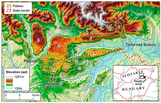
Figure 1.
Map of the study area. Karst plateaus are marked by ID numbers: Jelšavská (1); Koniarska (2); Plešivská (3); Bučina (4); Silická (5); Horný (6); Žl’ab (7); Bôrčianska (8); Zádielska (9); Jasovská (10); Kečovská-Haragistya (11); Nagyoldal (12); W-Alsó-hegy (13); E-Alsó-hegy (14); Szinpetri (15); Páska-bükk (16); Aggtelek (17); Rudabánya (18); Szalonna (19); Jósvafő (20).
2.2. Base Data
The main data sources of the present analyses are LiDAR databases. LiDAR data are available free of charge for Slovakia [91]. According to this portal, the technical parameters of the given territory (34-Rožňava) are as follows: scanning period: 28 April 2021–5 May 2021; vertical accuracy of cloud points: 0.08 m; positional accuracy of cloud points: 0.09 m; average density of last reflection points: 47/m2; and vertical accuracy of DTM (in ETRS89): 0.09 m. The raster DTM with a horizontal resolution of 1 m from LiDAR is also directly available from the database; thus, we used it in the analyses. As for the Hungarian side, the LiDAR database was created by the Envirosense Hungary Kft. on behalf of the Aggtelek National Park in August 2013. The data were provided to us by the Aggtelek National Park Directorate. The density of points classified as ground is 2 points/m2. It is relatively low because data collection was carried out during the vegetation period. Therefore, a DTM with a resolution of 2.5 m/px was created from the point cloud [18]. This database does not include the easternmost, relatively small plateaus of the Hungarian part of Aggtelek Karst (i.e., Rudabánya (18) and Szalonna (19) units; hereafter, numbers after local plateau names (Figure 1) are the “ID” numbers used in the figures and in the tables).
In addition to the LiDAR-based analysis, we also carried out the delineation of dolines based on topographic maps at a scale of 1:10,000 in both countries [92,93]. The outlines were delineated using the outermost-closed-contour method (see details in Section 2.3). If smaller closed depressions were clearly distinguishable within a large, complex depression, then we delineated the smaller features. In the Hungarian topographic maps, the contour interval is 5 m, but in the case of dolines, there are often secondary contour lines at 2.5 m vertical intervals. The Slovak topographic maps have contour intervals of 2 m.
To delineate the geological units, we used geological maps with a scale of 1:25,000 for the Hungarian parts and their associated map descriptions [60,64]. For the Slovakian parts, geological maps with a scale of 1:50,000 and their corresponding descriptions were used as a basis [61,62]. The scales are different, because these are the best publicly available geological maps in these countries.
2.3. Methodology
One of the crucial methodological issues in doline morphometry is the delineation of dolines. Dolines are small, closed depressions formed in karst areas. However, the lower and upper size limits are not clearly defined in the literature [15,17,94]. It is really not easy to specify a threshold diameter below which a small depression is considered a “random pit” and above which the form is regarded as a doline. Nevertheless, we have to set a lower limit in the procedure in order to exclude small depressions that are only due to minor random undulations of the surface (or of the DTM) and are not dolines. The upper limit is also ambiguous. Occasionally, dolines can grow very large, with diameters of 500 m or more [95]. If the bottom of a large, closed depression is not dissected by smaller forms, then it can still be considered a doline, even if its formation is more complex than that of simple dolines. For example, large, closed depressions are often found in valley sections that end in a stream sink. On the other hand, if a large, closed depression includes several smaller dolines, then the large form can be considered rather an “uvala”, and the smaller features within this can be delineated as dolines (see [96] for more details on uvalas). Nevertheless, “nested features” occur even in the case of smaller depressions [15]. These “nested features” can be formed by the coalescence of individual dolines or by the splitting of larger depressions into smaller parts. The question is how we delineate these forms. If two (or more) simple depressions within a larger depression are roughly the same size and are large enough to be considered dolines, then they should be delineated as individual dolines. However, when a tiny depression is found within a larger depression, then it is more realistic to delineate the larger depression as a doline. Finally, we note that complex (nested) depressions can be technically characterized by the “sinkhole rank” (see [15,97] for details).
Even if it is already decided which feature is considered to be a doline, there is still the question of where exactly to draw the outline of the feature. The outline of the doline can be determined by several methods (Figure 2). On topographic maps, the doline is indicated by closed contour lines (or occasionally by symbols). Thus, the edge of the doline can be defined most simply by the outermost closed contour (OCC). This is slightly lower compared to the lowermost point of the doline’s real rim. In fact, the vertical deviation is smaller than the value of the contour interval. Therefore, it necessarily represents a slightly narrower delineation than reality. At the same time, this instruction is clear and easy to follow for the digitizer, so this method is used quite often, especially if the basic data are topographic maps [7,21,26,31,98]. Another clear definition for doline delineation is the imaginary closed contour at the level of the lowermost point of the doline rim. This definition has become widespread in the case of DTM-based delineations [11,12,13,14,15,16,18]. Nonetheless, there is also an approach that states that the outline of the sinkhole is not necessarily horizontal. According to this definition, the outline of the sinkhole must be adjusted to the abrupt change in slope (that is, to the profile curvature maximum). However, the slopes of the doline edges can be so varied, and the slope transition often so gradual, that it is not possible to build a clear and universal definition based on this principle. As a result, this type of approach generally requires manual delineation, which leads to subjectivity. Thus, this method has not become widespread, although some researchers favor this definition despite its practical difficulties [20,98,99]. Finally, the outline of the doline can also be defined as the watershed belonging to its deepest point. This can unequivocally be performed on the basis of DTMs, but this method usually leads to much larger features than the real forms of dolines, except in the case of polygonal karsts consisting of closely packed dolines [10,16].
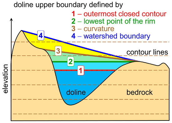
Figure 2.
Various doline delineation principles. The brown dashed lines indicate the elevation levels of the contour lines. For further explanation, see the text.
In our analysis, in the case of topographic maps, we delineated the dolines using the OCC method, while in the case of LiDAR-based DTMs, dolines were defined by the level of the lowermost point of the doline rim. The details of the delineation algorithm are presented in previous articles [12,15,18,97], so only the major steps and the flowchart (Figure 3) of the algorithm are presented here without further details.
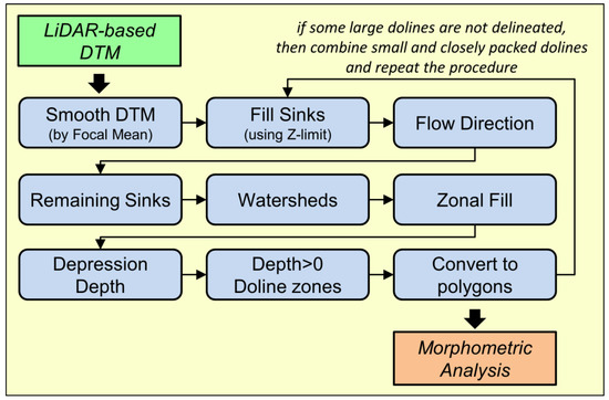
Figure 3.
Flowchart of the doline delineation algorithm. For further explanation, see the text.
- Smoothing of the DTM to remove spurious errors.
- Filling of pits smaller than true dolines (by setting the appropriate Z-limit). (In the case of a too-small Z-limit, there are many false positives, i.e., features outlined by the algorithm that are not true dolines. In the case of a too-large Z-limit, there are many false negatives, i.e., dolines that are not recognized by the algorithm. In [18], it was demonstrated that 1 m is the optimal value for Aggtelek Karst; thus, in the present analysis, the same value was used as the Z-limit.) The result is the “filled DTM”.
- Determination of flow directions based on the filled DTM.
- Identification of the remaining sinks (which are deeper than the above Z-limit): these are the “sink points”.
- Delineation of watersheds belonging to the sink points.
- Filling of depressions up to the level of the lowermost point of their rim. The result is the “zonal-filled DTM”.
- Calculation of the difference between the “zonal-filled DTM” and the “filled DTM”: this is the depth.
- Delineation of areas where the depth is larger than 0: these are the dolines (as raster data).
- Conversion of dolines into a polygon shape file for further analysis.
- Calculation of the morphometric characteristics of sinkholes.
Closed depressions, as mentioned above, are often “nested”. Handling these complex forms is a challenge. Kobal et al. [15] developed a procedure, the essence of which is to fill the depressions that have already been identified and then repeat the delineation procedure. As a result, we can also obtain the outlines of larger, complex features. In the present analysis, our experience was that after applying the delineation steps only once, we obtained the correct doline boundaries for most features. However, in certain cases, when a small doline was present in a larger feature, then only two (or more) tiny dolines were outlined, and the “true doline” (the larger feature) was missing from the database. This phenomenon is especially remarkable when comparing manual and automatic delineations (see Figure 4). To resolve this situation, after applying the algorithm once, we combined certain features. Dolines whose area or depth was too small (area less than 1000 m2 or depth less than 1 m) and were close to other sinkholes (distance less than 30 m) were filled, and the delineation steps were run again. Since the results obtained after the second round were satisfactory, we finished the delineation procedure after this second round.
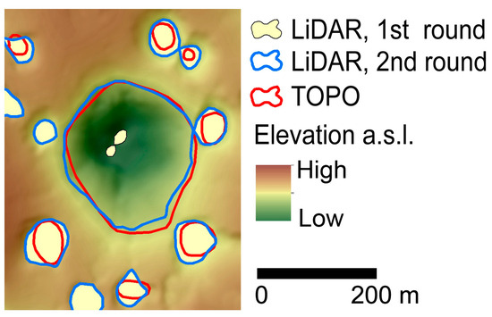
Figure 4.
A typical result of the delineation algorithm after the first and second rounds for a model area. The doline outlines based on the topographic map are also presented (TOPO). It is obvious that in the case of the large central doline, the delineation is incorrect after the first round; this is why the second round is necessary.
Morphometric parameters have been calculated using standard GIS tools. In the present paper, the following parameters are used: doline area (A), equivalent diameter (d, the diameter of the circle having the same area as the original form), depth (h, the elevation difference between the highest and lowest points of the doline), circularity (Circ), and volume (V). In the literature, there are several formulae for circularity; we used the following formula (after [19,100]), where P is the doline perimeter:
Circ = (4 × π × A)/P2
Based on DTMs, the volume can be calculated as the difference between the upper and lower envelope surfaces. Actually, the upper envelope surface is the horizontal polygon area of the doline. The lower envelope surface is the filled DTM (after the 2nd step of the algorithm). The volume is calculated as a sum:
where Apx is the area of one pixel, and hpx is the depth of the form in a given pixel. After some simple transformations, we obtain
where n is the number of pixels within the actual form. The mean depth (hmean) can be easily calculated in a GIS environment (e.g., by the Zonal Statistics as Table tool in ArcMap® 10.8 software), and the volume is calculated by multiplying this value with the area of the doline.
In this paper, a new morphometric parameter is also introduced: the 3D-shape parameter (k). The purpose is to characterize the ideal 3D geometric shape of dolines. In the literature, the shape of dolines is approximated as a cylinder, a bowl (or calotte), a cone, or a funnel (Figure 5). Naturally, these are idealized shapes, but they are often linked to genetic types. Namely, collapse sinkholes can be approximated by a cylinder, whereas solution dolines are closer to bowl or cone shapes. Before the advent of DTMs, the researchers selected a 3D shape typical of dolines in their research area, and the volume was calculated from the area and depth using the formula linked to the selected shape. Now, the situation is just the opposite: we are able to precisely calculate the volume using the LiDAR-based DTM, and we can assign an “idealized 3D shape” to the doline based on its volume. In order to carry this out, we have to take into account how the volume formulae change for the ideal 3D shapes. It is observed that the volume formulae have similar structures, and they can all be written in a general form:
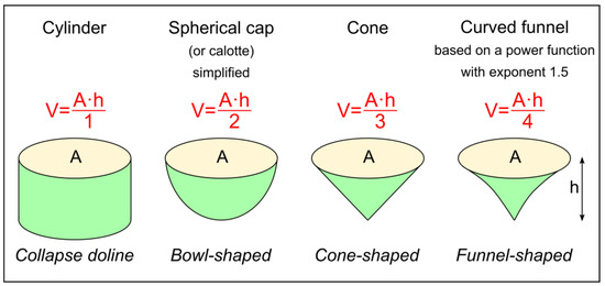
Figure 5.
Volume formulae of some idealized 3D shapes. Below the shapes, the names of the shapes when dolines are the subjects are given. The volume of the calotte is simplified here, but if the depth is relatively small with respect to the diameter, then the difference from the precise value is negligible.
In this formula, k reflects the ideal 3D shape of the given feature. Naturally, it is possible that a doline has exactly the same volume as the same-area and same-depth cone, while its true shape is quite different. Thus, we cannot say that if k is exactly 3, then the doline has a perfect cone shape. That is why we speak about an “idealized 3D shape”.
The parameters characterizing the spatial distribution of dolines are the doline density and the doline area ratio. The doline density is equal to the number of dolines divided by the study area. The doline area ratio is the total area of dolines divided by the study area. These parameters are sensitive to the size of the study area. In many studies, it is observed that “everything” is included in the study area, even sub-areas where dolines cannot occur at all for either lithological or topographical reasons. In such cases, we obtain low values for the whole area’s doline density, while the real situation is that the area that is actually covered by dolines can be characterized by a higher density. This problem can be solved by a doline density map, but if one wants to characterize the doline density with a single indicator value, then our proposal is that, as far as possible, one should take into account only those parts of the study area where the lithology allows for the formation of dolines and the slope angle is generally low. Naturally, these criteria should not be applied per pixel, but to larger contiguous areas. The numerical threshold of the slope angle should be determined on the basis of local conditions, but typically, the threshold value is around 10–12°, above which dolines occur only very rarely [9,35,53,55,101].
In order to compare doline density values among different areas, it is recommended to use the “same language”, i.e., common terms for doline density ranges. Recently, the classification of Pahernik [32] has been becoming widespread, according to which the doline density is “negligible” for 1–10 km−2, “small” for 10–30 km−2, “medium” for 30–60 km−2, “large” for 60–100 km−2, “very high” for 100–200 km−2, and “extremely high” for above 200 km−2. According to the literature, there are many well-karstified areas with a doline density of less than 10 km−2, including some plateaus of Aggtelek and Slovak Karsts; therefore, we recommend slightly modifying Pahernik’s too-strict designations, and our proposal is to call the 1–10 km−2 category “low” density, the 10–30 km−2 category “moderate” density, and the 60–100 km−2 category “high” density; for the other categories, we would leave the original terms of Pahernik.
3. Results
Hereafter, LiDAR-derived doline data are included in the analysis by default, except for the first point, where LiDAR-based and topographic map-based (hereinafter TOPO) data are compared. In the case of two plateaus (Rudabánya (18) and Szalonna (19)), no LiDAR data were available, so the parameters of the dolines were determined only on the basis of the topographic maps. For the whole karst area, the majority of dolines are located on the delineated plateaus (n = 4955). However, a small but non-negligible proportion of them cannot be assigned to the plateau terrains (n = 307). Nonetheless, when the context is the whole karst area, the data for “non-plateau dolines” are also included.
3.1. Features Identified in LiDAR versus TOPO Data
In the comparison, we focus on three parameters, doline density, doline area, and circularity, as these parameters characterize dolines from three different aspects: spatial distribution, size, and shape. Further on, considering the differences in data quality between the two countries, the results are also summarized by country. For the entire area, the LiDAR database contains 25% more dolines than TOPO. (In the case of Hungary, the surplus is 11%, whereas for Slovakia, it is 29%). Accordingly, the doline density is, on average, 25% higher when calculated based on LiDAR; however, this average value covers quite significant differences according to the plateaus (Figure 6). On the northern plateaus, LiDAR generally resulted in a larger surplus, in some cases drastically increasing the number of dolines (Jelšavská (1), Jasovská (10)), while the increase was smaller on the southern plateaus. There can be several reasons for this. On the one hand, this can be due to a bias, as the Hungarian LiDAR data have a lower resolution and lower quality than the Slovakian data. On the other hand, experience from our field trips also confirms that there are fewer small dolines in the Hungarian parts that do not appear on topographic maps, so the change compared to the TOPO data is smaller. As for the doline areas (Figure 6), the distributions of the two datasets are basically very similar. It is observed that although the LiDAR-based data contain the smallest-area dolines, TOPO dolines are, on average, somewhat smaller. The lower quartile, mean, and median values all support this observation. (For the whole study area, the median area of dolines is, on average, 17% larger for the LiDAR than for the TOPO dataset. For Hungary, this value is 13%, and for Slovakia, 18%). The reason for this is that, in the case of topographic maps, the border is defined by the outermost closed contour, which is typically somewhat lower than the elevation of the lowermost point of the rim of the doline; therefore, the area of TOPO dolines is smaller.
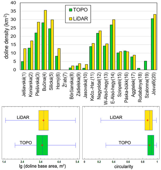
Figure 6.
A comparison of topographic map-based (TOPO) and LiDAR-based parameters. In the case of two plateaus (Rudabánya Mountains (18), Szalonna Karst (19)), no LiDAR data were available. Top: doline density; bottom left: box-whisker plot of doline area logarithms; bottom right: box-whisker plot of doline circularity. The vertical line in the box indicates the median, whereas red + indicates the mean values in the box-whisker plots.
Finally, regarding circularity (Figure 6), the diagram demonstrates that the shapes of TOPO dolines are more circular (for the whole study area, the median circularity of dolines is, on average, 3% smaller for the LiDAR than for the TOPO dataset; for Hungary, this value is 4%, and for Slovakia, 2%). The reason for this is that, according to cartographic principles, a kind of “generalizing/rounding effect” already prevails during the drawing of the contour lines in the map. In addition, during the digitization of the dolines, a further smoothing effect may have played a role. In contrast, during the LiDAR-based derivation, dolines are delineated by more realistic contours that better match the actual (observed) shapes of the dolines.
3.2. Doline Spatial Distribution Parameters
In print size, the dolines are too small to show all the features on one map, so here, we present a section that shows the Silická plateau (5) with the largest number of sinkholes (Figure 7).
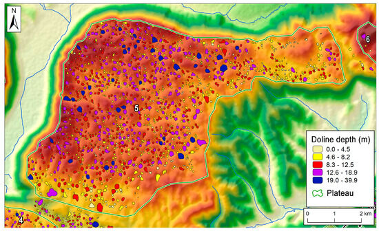
Figure 7.
Dolines of Silická plateau (5) delineated by the LiDAR-based methodology. Doline colors are according to depth. The numbers 4–6 refer to plateaus as in Figure 1 and Table 1. The map containing the whole Aggtelek Karst and Slovak Karst can be downloaded as a Supplementary File (Figure S1).
The spatial distribution of dolines can be well illustrated with a doline density map (Figure 8). This map shows that the north–central parts of the karst area are the most densely scattered with dolines. However, exceptions to this simple observation also exist; for example, Alsó-hegy (13, 14), Jósvafő plateau (20), and the northern tip of the Koniarska plateau (2) also have high-doline-density parts. In addition, a high-doline-density zone can be observed along the Gombasek–Silica tectonic line (between Silická (5) and Bučina (4) plateaus), which also continues to the NW on the Plešivská plateau (3). Regression analysis supports that the doline density is also influenced by the slope angle. At the level of plateau mean values, it is observed that there is a moderate (R2 = 0.50) negative correlation between the doline density and the mean slope angle (Figure 9). This means that, trend-wise, on the plateaus that are more horizontal, dolines are found in higher densities.
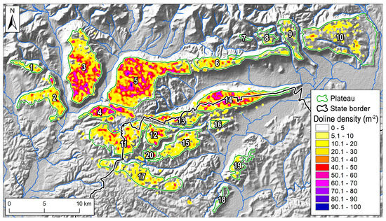
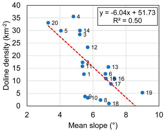
Table 1 demonstrates that there are significant differences in both the number and the density of dolines among the individual plateaus. There are no dolines at all on Žl’ab Mt. (7), and there are only a few dolines in the Rudabánya Mountains (18); thus, these are not doline-dotted plateaus. A rather low doline density (<8.8 km−2) characterizes Borčianska (8), Jasovská (10), Zádielska (9), Szalonna (19), and Aggtelek (17) karst plateaus. A moderate doline density (10.8–30 km−2) is typical of most plateaus, while the locally highest values (>28 km−2), though still only “medium” according to the general classification [32], are found on Plešivská (3), Silická (5), E-Alsó-hegy (14), Jósvafő (20), and Bučina (4) plateaus.

Table 1.
Some doline morphometric indicators of the plateaus of the study area: the number of dolines, doline density, doline area ratio, and the doline–area mean and median, n.d. means no data.
As already mentioned, the general slope angle significantly determines where sinkholes can form. Examining this question on the basis of the DTM, we calculated the general slope of the terrain in the doline centers. It is important to look at the general slope because the actual slope in the doline center is theoretically 0° (since it is a local minimum). Therefore, to calculate the general slope, instead of LiDAR, the 1″ resolution SRTM dataset was used [102]. But even the SRTM was further smoothed by a mean filter with a radius of three and five cells, and the slope angle was calculated based on these filtered DTMs, too, in order to obtain the general slope of the terrain. Thereafter, the distribution of the general slope angle of doline centers was examined. There are only minor differences among the distributions based on the unsmoothed, three-cell smoothed, and five-cell smoothed 1′′ resolution SRTM data. Our goal is to determine the slope angle threshold that limits the formation of sinkholes; thus, the upper percentiles of the slope angle distributions are presented in Table 2. It highlights that there are only very few dolines formed on terrains steeper than 12°, and one can say that 90% of sinkholes are formed on terrains with a general slope of less than 7–8° (the exact value depends on filtering).
Table 2.
The percentile values of the general slope angles measured in doline centers. Slope values refer to the general slope of the terrain calculated from the unsmoothed and mean-filtered SRTM 1” DTM.
In addition to the slope angle, geological settings also influence the location of sinkholes: the formation of high-doline-density zones can be clearly observed along some fault lines. Based on the Slovak and Hungarian geological maps, three-quarters of dolines were formed on Wetterstein Limestone, whereas the second most important bedrock is Steinalm Limestone (Table 3). Further on, dolines also occur at a few percent on the following lithologies: Wetterstein Dolomite, Reifling Limestone, Gutenstein Limestone, Gutenstein Dolomite, Gutenstein Formation undistinguished, deluvial sediments, Waxeneck Limestone, and Szin Beds. As Table 3 demonstrates, Wetterstein Limestone is more favorable for doline evolution than other rocks, because it has a higher share of dolines than of area. Steinalm Limestone and Reifling Limestone have the same share of dolines as of area. All other lithologies have lower shares of doline than of area.
Table 3.
Distribution of dolines according to lithology. Lithologies with less than 0.9% of all dolines are not shown.
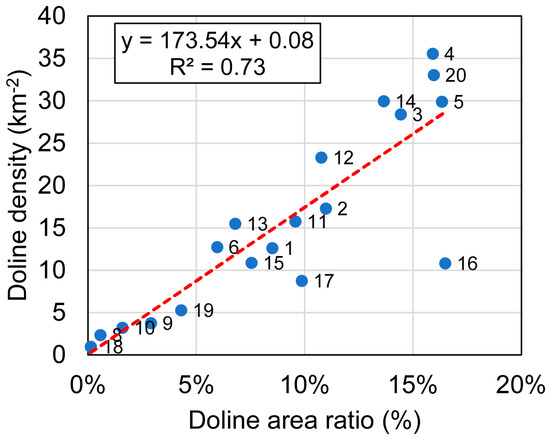
An indicator similar to the doline density is the doline area ratio, which expresses the proportion of the surface that is covered by dolines. The difference with respect to the doline density is that larger dolines may create greater coverage, even at a lower doline density. According to Figure 10, a high area ratio due to large dolines is the most characteristic of the southern and western parts of the karst region, as the most obvious outliers are the Aggtelek (17) and Páska-bükk (16) plateaus, but the Szinpetri (15), Jelšavská (1), and Koniarska (2) plateaus also advance in the doline area ratio ranking with respect to the doline density rank. A possible explanation for this fact is that the development of the dolines along the boundaries of the karst areas was more intensive due to streams flowing from non-karst areas to the karst terrain; thus, the dolines could grow larger in these parts. In the case of Páska-bükk (16), there is a special reason: one of the largest dolines in the entire karst region is found here (A = 125,784 m2), which results in an outstanding “doline area ratio”. The difference between the interpretation of the doline density and the doline area ratio is also reflected in Figure 11. In the case of similar-sized dolines, the relationship between the doline density and the doline area ratio would be a simple line with R2 close to 1. However, as Figure 11 demonstrates, the strength of the relationship is strong but not very strong. Points above the regression line mean plateaus where the doline density is higher than expected from the doline area ratio due to the high proportion of relatively small dolines. On the other hand, points below the line mark plateaus, where relatively large dolines significantly increase the doline area ratio, even if the doline density is not so high. The most extreme example is the Páska-bükk (16) plateau due to the aforementioned reason.
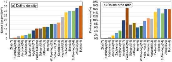
Figure 10.
Doline density (a) and doline area ratio (b) by plateau sorted by doline density.
3.3. Doline Area Empirical Distributions
The mean doline area for the whole study area is 5514 m2, which corresponds to an equivalent diameter of 84 m. However, since the size distribution of the sinkholes is highly skewed, the median value better expresses the size of the “typical doline”. In the study area, this is 3638 m2, which corresponds to a diameter of 68 m. As described in the doline area ratio section, the Koniarska (2), Jelšavská (1), Szinpetri (15), Zádielska (9), Szalonna (19), and especially the Aggtelek (17), and Páska-bükk (16) plateaus can be characterized by larger dolines. In contrast, the type areas of smaller sinkholes (in addition to the Bôrčianska(8) and Rudabánya(18) units, which have hardly any sinkholes) are the Alsó-hegy (13, 14) and Bučina (4) plateaus. The doline areas according to the bedrock are presented in Figure 12 for the important (i.e., with a proportion of at least 0.9%) lithological categories. It shows that within the most common Wetterstein Limestone category (n = 3834), smaller sinkholes dominate. The dolines formed on Wetterstein Dolomites (n = 154) are similar in median value but somewhat larger in mean value. The size of the dolines formed on Reifling Limestone (n = 119) and Steinalm Limestone (n = 532) occupies an intermediate position, and finally, the largest areas are typical of the dolines formed on Gutenstein Formations (n = 286 altogether).
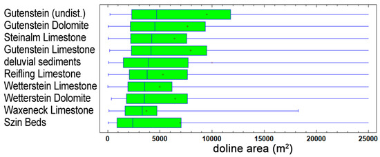
Figure 12.
Box-whisker plots of the doline area categorized by bedrock. A vertical line indicates the median value, and “+” is the mean value.
Regarding the study area, the results support that the statistical distribution of doline areas can be well modeled by the lognormal distribution. Table 4 indicates that, for most plateaus, the statistical tests (chi-square and Kolmogorov–Smirnov) confirmed that the logarithm of the data shows a normal distribution; therefore, the distribution of the original data is lognormal. For the sake of brevity, only the six plateaus with the most sinkholes are shown in the diagrams (Figure 13). As for Plešivská (3), Silická (5), and E-Alsó-hegy (14), if the smallest features detected as dolines are omitted using 200 m2 (equivalent diameter ca. 8 m) as a lower limit for the doline area, then the statistical tests support the lognormal distribution even in these cases. This means that only a few small features (n = 17, 20, and 12 for Plešivská (3), Silická (5), and E-Alsó-hegy (14), respectively) obscure the lognormal nature of the distributions for these plateaus.
Table 4.
The test results of doline area distribution fitting for the study area plateaus. Chi-square and Kolmogorov–Smirnov (K-S) tests were used for the log-transformed data. The null hypothesis is that the log-transformed data fit a normal distribution. If p > 0.05, then the null hypothesis cannot be rejected, n.d. means no data.
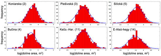
Figure 13.
Empirical distributions of the doline area after log transformation for the six plateaus with the most sinkholes (Koniarska, Plešivská, Bučina, Silická, Kečovská–Haragistya, E-Alsó-hegy). Blue lines indicate the fitted normal distribution (after the log transformation).
The possibility of a power-law distribution was also examined. Graphs showing the cumulative frequency distribution for the six plateaus with the most sinkholes were also created (Figure 14). If a logarithmic scale is used on both axes and the power-law distribution is true, then the points must fit on a straight line [17,39]. The results indicate that only a limited part of the graphs fulfills linearity; i.e., the power function fits only a limited part of the original data. The lower limit of linearity cannot be clearly determined based on these graphs, because the slopes of the functions change gradually, but as an approximation, one can say that the graph is linear for doline areas above 5000 m2. This value is much higher than the threshold used during the doline delimitation procedure; thus, it is not an artifact. Therefore, it is stated that the power-law distribution is not suitable to model doline area distributions in this karst terrain.
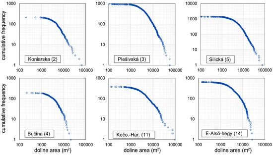
Figure 14.
Cumulative frequency distributions of the doline area on a logarithmic scale for the six plateaus with the most sinkholes.
3.4. Parameters Characterizing the Vertical Shape
Among the parameters characterizing the vertical shape of dolines, the depth and the depth-to-diameter ratio were calculated (Table 5). There are significant differences in both parameters according to the plateau and according to the bedrock, too. In both absolute and relative terms, shallow dolines can be found in the Rudabánya (18), Bôrčianska (8), Jósvafő (20), Zádielska (9), and Jasovská (10) units. It means that the average depth of dolines on these plateaus is less than 4 m. The other extreme is represented by Bučina (4) and E-Alsó-hegy (14), where the average depth of dolines approaches 10 m, and the depth-to-diameter ratio is also outstanding in these places (0.13–0.14). In the case of Páska-bükk (16), the average depth is greatly increased by the giant doline of the plateau, but since its areal extent is also large, the depth-to-diameter ratio is not outstanding here. In geological terms, Figure 15 illustrates that the Wetterstein Limestone, which represents the vast majority of dolines, has the largest depth-to-diameter ratio; i.e., the “typical”, relatively steep-sided dolines are characteristic of this bedrock. Compared to the above bedrock, the dolines formed on Steinalm Limestone or Reifling Limestone are somewhat shallower, and the dolines formed on Gutenstein Formations, Waxeneck Limestone, and Wetterstein Dolomite are even shallower. Finally, the shallowest features can be associated with the Szin Beds and the deluvial sediments. These differences can be explained by geomorphological processes.
Table 5.
Vertical doline parameters: depth, depth-to-diameter ratio, volume, 3D-shape parameter (k), and mean denudation. (Since LiDAR data were not available for Rudabánya (18) and Szalonna (19) mountains, these parameters were not calculated for these units.) n.d. means no data.
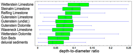
Figure 15.
A box-whisker plot of the doline depth-to-diameter ratio according to lithological categories. A vertical line indicates the median value, and “+” is the mean value.
The volume of dolines essentially expresses how much the given doline “contributed” to the karst denudation. If, for a plateau, the total volume of dolines is divided by the area of the plateau, then we obtain a mean denudation thickness that is directly due to doline growth. The mean volume, the 3D-shape parameter, and the mean denudation thickness values of the plateaus are presented in Table 5.
The volumes of the dolines, as well as the mean denudation thickness, show extreme values for Páska-bükk (16), which is again attributed to the giant doline on this plateau. Apart from this, the plateaus in the western and southern parts of the karst can be characterized by large-volume dolines. These are the plateaus where doline areas are also outstanding (Aggtelek (17), Jelšavská (1), Szinpetri (15), and Koniarska (2) plateaus). However, from the viewpoint of mean denudation thickness, the doline density is more influential than the doline size (either area or volume). In statistical terms, if the extreme value of Páskabükk (16) is omitted, then R2 between the mean denudation thickness and doline density is 0.66, while R2 between the mean denudation thickness and mean doline area is only 0.03, and R2 between the mean denudation thickness and mean doline volume is 0.23. As a result, Bučina (4), E-Alsó-hegy (14), Silická (5), and Plešivská (3) plateaus have high denudation thickness values. In contrast, the northeastern plateaus (Bôrčianska (8), Zádielska (9), Jasovská (10)) show quite low values. It is difficult to interpret the magnitude of the volume in itself, but the value of the mean denudation thickness expressed in meters is already more tangible. It is observed that this value varies between 0.4 and 0.8 m. These low values are interpreted in Section 4.
As for the 3D shapes of the dolines, there are significant differences among the plateaus (Figure 16). Overall, the diagram demonstrates that the 3D shape of most dolines falls between the bowl (calotte) and the cone. According to the diagram, dolines close to cylindrical shape are very rare, which is in agreement with the settings of this karst area, where collapse sinkholes are almost absent. In general, the spatial distribution of the 3D-shape parameter suggests that bowl-shaped dolines are more typical in the southern parts of the karst region, while in the northern parts, there is a shift toward the cone shape. However, with the exception of the Jasovská (10) and Zádielska (9) plateaus, even in the northern parts, the bowl shape dominates. Close-to-funnel-type dolines occur only as individual outliers on the northern plateaus. Since the highest plateaus have a higher proportion of cone- or funnel-type dolines, the 3D-shape parameter is slightly but significantly correlated with the elevation above sea level (R = 0.12).
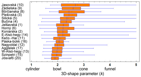
Figure 16.
A box-whisker plot of the doline 3D-shape parameter (k) by plateau. A vertical line indicates the median value, and “+” is the mean value.
4. Discussion
First, we discuss the accuracy of the doline extraction method. The question is what we consider a “true value” or “reference data”. Reliable field data about doline locations with large sample sizes are not available to us, but our several decades of field experience suggests that 1:10,000-scale topographic maps are of relatively high quality for this area in terms of doline locations. Naturally, dolines smaller than 30 m cannot be proportionately represented at this scale, but such small dolines are negligible in the area according to our field experience. If the topographic maps are considered reference data, it is argued that the LiDAR-based delineation is better than the reference itself. Almost all dolines in the topographic maps are recognized based on the LiDAR dataset, and even 25% more dolines are delineated starting from LiDAR. This can be compared to the results of [20]. They made a thorough comparison of different methods for a smaller subunit (the south-western part of the Silická planina) of Slovak Karst. In brief, they obtained the following results in terms of doline numbers: using the outermost closed contour method based on 1:10,000-scale topographic maps, they obtained 432 dolines. The simple DEM-based sink-fill algorithm resulted in 657 dolines, whereas their water flow simulation algorithm resulted in 592 dolines. Finally, the DEM-based manual delineation by experts resulted in 622 dolines (and they accepted this last one as the “true value”). We tried to outline the same study area as in [20], though some minor differences exist in the north. The results show that for the same area, our database contained 476 dolines from the topographic map and 612 dolines based on LiDAR. This means that the doline extraction accuracy in the present paper is similar to that in [20]. From a theoretical perspective, it is possible to estimate the accuracy related to the original LiDAR dataset. According to the provider of the Slovak LiDAR dataset, both the positional and vertical accuracies of cloud points are 0.08–0.09 m. As for the derived DTM accuracy, there is no such value published, but given the accuracy of cloud points, it can be assumed that one pixel has a positional accuracy of 1 m (or better). In that case, the horizontal accuracy of the extracted feature vertices is also ca. 1 m. The minimum size of a depression in the DTM is 3 × 3 pixels, but small random errors can also influence it. However, we believe that 5 × 5-pixel (or larger) depressions (with a Z-limit of 1 m) can be reliably identified by the algorithm. In the case of the Hungarian LiDAR dataset, we do not have information about the positional accuracy of cloud points, but starting from a pixel size of 2.5 m, we can say that depressions larger than 12.5 m × 12.5 m can be reliably identified.
In the study area, the distributions of the doline area have a tendency toward lognormal distributions for most of the plateaus. To discuss this fact, it is worth recalling the general interpretation of the lognormal distribution. The lognormal distribution can be observed in the case of several natural phenomena (see [103]). Quite often, there is a “multiplicative process” behind the lognormal distribution. This means that the size of the individuals of a studied population changes by a random multiplier per time unit, so the growth rate itself is independent of the size, but the actual growth is proportional to the size of the individual in the previous step. This process and the resulting lognormal distribution applied to economic companies were already described in the 1930s [104,105]. However, Mitzenmacher [106] also proved that if we slightly change the conditions of a multiplicative model, for example, by setting a threshold or summing up the effects of several such processes, then the result will no longer be lognormal, but a power-law distribution. Barabási [107] calls the lognormal distribution a “crossover distribution” and points out that there is a debate in many scientific fields about whether the power-law distribution or the lognormal distribution fits the observations better. Thus, in future research on karst areas, the examination of the empirical distribution of the doline area is definitely justified in order to answer this question. In any case, based on our data, it is assumed that the growth of dolines can be described by a multiplicative model. The essence of this model is that, during the evolution of dolines, random effects are multiplied (and not added up). It seems to be a feasible approach if it is assumed that the growth of the doline is proportional to the precipitation falling into its area, the infiltrating percentage of precipitation, and the dissolution capacity of the infiltrating water. In other words, the growth is proportional to the size, but the growth rate itself is influenced by size-independent and random effects (precipitation, infiltration percentage, dissolution capacity). Further details of a doline growth model are beyond the scope of this paper.
Another parameter that deserves discussion is the mean denudation thickness value calculated from doline volumes. This can be used to calculate the mean denudation rate (i.e., the denudation per time unit) only if the formation time of the dolines is known [108]. To determine the latter, exposure age calculations applied to karst surfaces can be a solution [109,110,111,112,113,114]. The spatial pattern of denudation is still poorly understood, but it is supported that doline centers have higher denudation rates [109,115]. So far, there are only a few measurement data on how the denudation of doline centers and the interdoline ridges relate to each other. If the interdoline ridges have not yet been narrowed, then it may be assumed that they preserve the pre-denudation surface. This is not necessarily true, but let us assume this situation as a hypothesis. Then, the denudation of the interdoline terrains is close to zero. In this hypothetical case, the absolute value of surface denudation due to karst processes is well approximated by the total volume of dolines. As mentioned above, the duration of doline evolution is not known exactly for the study area, but the literature agrees that karst processes became dominant in this area during the Quaternary [65,75,76,77,79]. Thus, with a very rough estimation, if the duration of doline evolution is estimated to be 2 million years, then the rate of surface denudation directly due to karst processes is on the order of 0.2–0.4 m/Ma, which is an extremely slow rate. This explains why karst plateaus are so often higher than their non-karstic surroundings. Nevertheless, in the case of Aggtelek Karst and Slovak Karst, differential tectonic uplift also contributed (probably with a much higher rate) to the local prominence of karst plateaus [85]. In addition, it is noted that the denudation values calculated from the dissolved carbonate content of the waters flowing out of the karst springs represent the “full 3D denudation” of the karst, including the corrosion of karst caves within the rock mass; therefore, these “full 3D denudation” values are significantly greater than the denudation calculated merely from the lowering of the surface [116,117]. Anyway, the complex discussion of karst denudation is another topic, but doline morphometrical results can contribute to this topic.
5. Conclusions
In our quantitative analysis, doline morphometric data derived from topographic maps (TOPO) and from the LiDAR-derived DTM were compared for the Aggtelek Karst and Slovak Karst. It is found that these two datasets fit each other relatively well, but based on the LiDAR-derived DTM, the doline density proved to be 25% higher. As for doline size, the LiDAR-based dataset contains more tiny dolines than the TOPO (i.e., dolines missing from the topographic map), but the average size of the LiDAR-derived dolines is larger than that of the TOPO dolines, which can be explained by the different delineation procedures (DTM-derived versus OCC). The circularity of the shapes of TOPO sinkholes is closer to a circle than that of LiDAR-derived sinkholes. This is attributed to the smoothing effect during map creation and digitization. These results provide a clue to re-evaluate doline morphometric data obtained on the basis of topographic maps in earlier decades of doline morphometrical research. However, these results can be applied to other areas only with caution, since the scale and quality of the topographic maps, the resolution and quality of the LiDAR data, and the typical sizes of sinkholes influence these findings.
Comparing the Aggtelek Karst and Slovak Karst to other temperate-climate doline karsts, it is stated that the plateaus of this area are in the middle range, considering their doline parameters. These plateaus are characterized by low (5–10 km−2), moderate (10–30 km−2), and medium (30–35 km−2) doline densities. Bučina (4), E-Alsó-hegy (14), and Jósvafő (20) plateaus have the most outstanding values. Sinkholes cover 2–17% of the area of the plateaus. From this point of view, the record holder of the study area is the Silická plateau, which has relatively large and densely packed sinkholes. The location of dolines is strongly determined by the general slope angle, in addition to the geological characteristics. Sinkholes above a general slope of 12° are only rarely found, and 90% of the sinkholes are formed on terrains with a general slope of less than 8°. Among the geological conditions, the distribution of the Wetterstein Limestone is the most decisive for the study area, as 72.9% of the dolines are located on this bedrock. It is also observed that dolines formed on this bedrock are typically smaller in size than in the case of other lithologies.
The statistical distribution of the doline area can be relatively well modeled by a lognormal distribution for most plateaus, while the power law does not fit well to the cumulative distribution.
Doline depth is influenced by both the position and the dominant bedrock of the plateau. The sinkholes are shallower on the southern and lower plateaus, while the sinkholes with the largest depth-to-diameter ratios are found in the central and northern parts, primarily on Wetterstein Limestone. Based on this parameter, the plateaus of Bučina (4) and E-Alsó-hegy (14) can be highlighted as the lands with the deepest sinkholes.
Doline volume was used to calculate the mean denudation thickness value, which is in the range of 0.4–0.8 m for most of the examined plateaus. It is important to note that this is an absolute value, not a rate indicating change over time.
The volume of sinkholes calculated on the basis of the DTM also provides an opportunity to introduce a new type of parameter characterizing the 3D shape. This is the 3D-shape parameter (k), which nominally shows how much the expression A·h (area·depth) must be divided by to obtain the volume of the sinkhole. As for its interpretation, the parameter k shows whether the 3D shape of the doline is closer to a cylinder, a bowl (calotte), a cone, or a funnel. In the case of Aggtelek Karst and Slovak Karst, the 3D shape of most dolines falls between a bowl (calotte) and a cone. Bowl-shaped sinkholes are more typical in the southern parts, whereas in the northern parts, there is a shift toward the cone shape.
Supplementary Materials
The following supporting information can be downloaded at https://www.mdpi.com/article/10.3390/rs16050737/s1: Figure S1: Map of dolines of Aggtelek Karst and Slovak Karst. Karst plateaus are marked by ID number: Jelšavská (1); Koniarska (2); Plešivská (3); Bučina (4); Silická (5); Horný (6); Žl’ab (7); Bôrčianska (8); Zádielska (9); Jasovská (10); Kečovská-Haragistya (11); Nagyoldal (12); W-Alsó-hegy (13); E-Alsó-hegy (14); Szinpetri (15); Páska-bükk (16); Aggtelek (17); Rudabánya (18); Szalonna (19); Jósvafő (20).
Author Contributions
Conceptualization and methodology: T.T.; investigation: T.T. and L.M.; data curation: T.T.; validation: T.T. and B.S.; visualization: T.T.; writing: T.T.; writing—review and editing: L.M. and B.S. All authors have read and agreed to the published version of the manuscript.
Funding
This research received no external funding.
Data Availability Statement
Data are contained within the article.
Acknowledgments
The authors thank Aggtelek NP for providing the LiDAR dataset for Aggtelek Karst. The authors are indebted to the reviewers for their constructive comments and suggestions that improved the manuscript.
Conflicts of Interest
The authors declare no conflicts of interest.
References
- Cvijić, J. Das Karstphänomen. Versuch Einer Morphologischen Monographie; Hölzel: Wien, Austria, 1893; Volume 5, pp. 218–329. [Google Scholar]
- Ford, D.; Williams, P.D. Karst Hydrogeology and Geomorphology; John Wiley & Sons: Hoboken, NJ, USA, 2013. [Google Scholar]
- Williams, P.W. Illustrating Morphometric Analysis of Karst with Examples from New Guinea. Z. Für Geomorphol. 1971, 15, 40–61. [Google Scholar] [CrossRef]
- Williams, P.W. Morphometric Analysis of Polygonal Karst in New Guinea. GSA Bull. 1972, 83, 761–796. [Google Scholar] [CrossRef]
- Orndorff, R.C.; Weary, D.J.; Lagueux, K.M. Geographic Information Systems Analysis of Geologic Controls on the Distribution on Dolines in the Ozarks of South-Central Missouri, USA. Acta Carsol. 2000, 29, 161–175. [Google Scholar] [CrossRef]
- Gao, Y.; Alexander, E.C., Jr.; Tipping, R.G. The Development of a Karst Feature Database for Southeastern Minnesota. J. Cave Karst Stud. 2002, 64, 51–57. [Google Scholar]
- Denizman, C. Morphometric and Spatial Distribution Parameters of Karstic Depressions, Lower Suwanee River Basin, Florida. J. Cave Karst Stud. 2003, 65, 29–35. [Google Scholar]
- Florea, L.J. Using State-Wide GIS Data to Identify the Coincidence Betwen Sinkholes and Geologic Structure. J. Cave Karst Stud. 2005, 67, 120–124. [Google Scholar]
- Faivre, S.; Pahernik, M. Structural Influences on the Spatial Distribution of Dolines, Island of Brac, Croatia. Z. Für Geomorphol. 2007, 51, 487–503. [Google Scholar] [CrossRef]
- Telbisz, T.; Dragušica, H.; Nagy, B. Doline Morphometric Analysis and Karst Morphology of Biokovo Mt (Croatia) Based on Field Observations and Digital Terrain Analysis. Hrvat. Geogr. Glas. 2009, 71, 5–22. [Google Scholar] [CrossRef]
- Gallay, M.; Kaňuk, J.; Petrvalská, A. Využitie Údajov Leteckého Laserového Skenovania vo Výskume Krasovej Krajiny Na Slovensku—Na Príklade Východnej Časti Slovenského Krasu. (Using the Airborne Laser Scanning Data in Studying the Karst Landscape of Slovakia—Case Study of the Eastern Part of the Slovak Karst). Slov. Kras 2013, 51, 99–108. [Google Scholar]
- Obu, J.; Podobnikar, T. Algoritem Za Prepoznavanje Kraških Kotanj Na Podlagi Digitalnega Modela Reliefa (Algorithm for Karst Depression Recognition Using Digital Terrain Model). Geod. Vestn. 2013, 57, 260–270. [Google Scholar] [CrossRef]
- Rahimi, M.; Alexander, C. Locating Sinkholes in LiDAR Coverage of a Glacio-Fluvial Karst, Winona County, MN. In Proceedings of the Full Proceedings of the Thirteenth Multidisciplinary Conference on Sinkholes and the Engineering and Environmental Impacts of Karst, Carlsbad, NM, USA, 6–10 May 2013; National Cave and Karst Research Institute: Carlsbad, NM, USA, 2013; pp. 469–480. [Google Scholar]
- Zhu, J.; Taylor, T.P.; Currens, J.C.; Crawford, M.M. Improved Karst Sinkhole Mapping in Kentucky Using LiDAR Techniques: A Pilot Study in Floyds Fork Watershed. J. Cave Karst Stud. 2014, 76, 207–216. [Google Scholar] [CrossRef]
- Kobal, M.; Bertoncelj, I.; Pirotti, F.; Dakskobler, I.; Kutnar, L. Using Lidar Data to Analyse Sinkhole Characteristics Relevant for Understory Vegetation under Forest Cover—Case Study of a High Karst Area in the Dinaric Mountains. PLoS ONE 2015, 10, e0122070. [Google Scholar] [CrossRef]
- Bauer, C. Analysis of Dolines Using Multiple Methods Applied to Airborne Laser Scanning Data. Geomorphology 2015, 250, 78–88. [Google Scholar] [CrossRef]
- Jeanpert, J.; Genthon, P.; Maurizot, P.; Folio, J.-L.; Vendé-Leclerc, M.; Sérino, J.; Join, J.-L.; Iseppi, M. Morphology and Distribution of Dolines on Ultramafic Rocks from Airborne LiDAR Data: The Case of Southern Grande Terre in New Caledonia (SW Pacific). Earth Surf. Process. Landf. 2016, 41, 1854–1868. [Google Scholar] [CrossRef]
- Telbisz, T.; Látos, T.; Deák, M.; Székely, B.; Koma, Z.; Standovár, T. The Advantage of Lidar Digital Terrain Models in Doline Morphometry Compared to Topographic Map Based Datasets—Aggtelek Karst (Hungary) as an Example. Acta Carsol. 2016, 45, 5–18. [Google Scholar] [CrossRef]
- Wu, Q.; Deng, C.; Chen, Z. Automated Delineation of Karst Sinkholes from LiDAR-Derived Digital Elevation Models. Geomorphology 2016, 266, 1–10. [Google Scholar] [CrossRef]
- Hofierka, J.; Gallay, M.; Bandura, P.; Šašak, J. Identification of Karst Sinkholes in a Forested Karst Landscape Using Airborne Laser Scanning Data and Water Flow Analysis. Geomorphology 2018, 308, 265–277. [Google Scholar] [CrossRef]
- Verbovšek, T.; Gabor, L. Morphometric Properties of Dolines in Matarsko Podolje, SW Slovenia. Environ. Earth Sci. 2019, 78, 396. [Google Scholar] [CrossRef]
- Bauer, C.; Wagner, T. From Landform Inventories to Landscape Evolution?—Karst Development in the Central Styrian Karst (Austria). Geomorphology 2024, 447, 109024. [Google Scholar] [CrossRef]
- Látos, T.; Telbisz, T. LiDAR És UAV Alapú Digitális Domborzatmodellek Összevetése Töbör-Morfometria Szempontjából a Jósvafői-Fennsík Példáján. Karsztfejlődés 2018, 23, 19–30. [Google Scholar] [CrossRef]
- Oliveira, S.; Moura, D.; Boski, T.; Horta, J. Coastal Paleokarst Landforms: A Morphometric Approach via UAV for Coastal Management (Algarve, Portugal Case Study). Ocean Coast. Manag. 2019, 167, 245–261. [Google Scholar] [CrossRef]
- Menezes, D.F.; Bezerra, F.H.; Balsamo, F.; Arcari, A.; Maia, R.P.; Cazarin, C.L. Subsidence Rings and Fracture Pattern around Dolines in Carbonate Platforms—Implications for Evolution and Petrophysical Properties of Collapse Structures. Mar. Pet. Geol. 2020, 113, 104113. [Google Scholar] [CrossRef]
- Utlu, M.; Öztürk, M.Z. Comparison of Morphometric Characteristics of Dolines Delineated from TOPO-Maps and UAV-DEMs. Environ. Earth Sci. 2023, 82, 165. [Google Scholar] [CrossRef]
- Ford, D. Jovan Cvijić and the Founding of Karst Geomorphology. Environ. Geol. 2007, 51, 675–684. [Google Scholar] [CrossRef]
- Kemmerly, P.R. Spatial Analysis of a Karst Depression Population: Clues to Genesis. GSA Bull. 1982, 93, 1078–1086. [Google Scholar] [CrossRef]
- Troester, J.W.; White, E.L.; White, W.B. A Comparison of Sinkhole Depth Frequency Distributions in Temperate and Tropic Karst Regions. In Proceedings of the Multidisciplinary Conference on Sinkholes. 1, Orlando, FL, USA, 15–17 October 1984; pp. 65–73. [Google Scholar]
- Kemmerly, P.R. Exploring a Contagion Model for Karst-Terrane Evolution. GSA Bull. 1986, 97, 619–625. [Google Scholar] [CrossRef]
- Telbisz, T. Új Megközelítések a Töbör-Morfológiában Az Aggteleki-Karszt Példáján (New Perspectives in Doline-Morphometry—Aggtelek Karst as an Example). Földrajzi Közlemények 2001, 125, 95–108. [Google Scholar]
- Pahernik, M. Spatial Density of Dolines in the Croatian Territory. Hrvat. Geogr. Glas. 2012, 74, 5–26. [Google Scholar] [CrossRef]
- Veress, M.; Telbisz, T.; Tóth, G.; Lóczy, D.; Ruban, D.A.; Gutak, J. Glaciokarsts; Springer Geography; Springer International Publishing: Cham, Swizterland, 2019; ISBN 978-3-319-97291-6. [Google Scholar]
- Gao, Y.; Alexander, E.C.; Barnes, R.J. Karst Database Implementation in Minnesota: Analysis of Sinkhole Distribution. Environ. Geol. 2005, 47, 1083–1098. [Google Scholar] [CrossRef]
- Plan, L.; Decker, K. Quantitative Karst Morphology of the Hochschwab Plateau, Eastern Alps, Austria. Z. Geomorphol. Suppl. Issues 2006, 147, 29–54. [Google Scholar]
- Brinkmann, R.; Parise, M.; Dye, D. Sinkhole Distribution in a Rapidly Developing Urban Environment: Hillsborough County, Tampa Bay Area, Florida. Eng. Geol. 2008, 99, 169–184. [Google Scholar] [CrossRef]
- Pardo-Iguzquiza, E.; Pulido-Bosch, A.; Lopez-Chicano, M.; Duran, J. Morphometric Analysis of Karst Depressions on a Mediterranean Karst Massif. Geogr. Ann. Ser. A Phys. Geogr. 2016, 98, 247–263. [Google Scholar] [CrossRef]
- Pardo-Igúzquiza, E.; Dowd, P.A.; Durán, J.J.; Robledo-Ardila, P. A Review of Fractals in Karst. Int. J. Speleol. 2018, 48, 11–20. [Google Scholar] [CrossRef]
- Pardo-Igúzquiza, E.; Dowd, P.A.; Telbisz, T. On the Size-Distribution of Solution Dolines in Carbonate Karst: Lognormal or Power Model? Geomorphology 2020, 351, 106972. [Google Scholar] [CrossRef]
- Šušteršič, F. Are “Collapse Dolines” Formed Only by Collapse? Acta Carsol. 2000, 29, 213–230. [Google Scholar] [CrossRef]
- Šušteršič, F. A Power Function Model for the Basic Geometry of Solution Dolines: Considerations from the Classical Karst of South-Central Slovenia. Earth Surf. Process. Landf. 2006, 31, 293–302. [Google Scholar] [CrossRef]
- Yakar, M.; Yilmaz, H.M.; Mutluoglu, O. Performance of Photogrammetric and Terrestrial Laser Scanning Methods in Volume Computing of Excavtion and Filling Areas. Arab. J. Sci. Eng. 2014, 39, 387–394. [Google Scholar] [CrossRef]
- Lu, B.; Zhu, J.; Ge, Y.; Chen, Q.; Wen, Z.; Liu, G.; Li, L. Automated Determination of the Volume of Loose Engineering Deposits Using Terrestrial Laser Scanning. Remote Sens. 2023, 15, 4604. [Google Scholar] [CrossRef]
- Slattery, K.T.; Slattery, D.K.; Peterson, J.P. Road Construction Earthwork Volume Calculation Using Three-Dimensional Laser Scanning. J. Surv. Eng. 2012, 138, 96–99. [Google Scholar] [CrossRef]
- Bisson, M.; Spinetti, C.; Andronico, D.; Palaseanu-Lovejoy, M.; Fabrizia Buongiorno, M.; Alexandrov, O.; Cecere, T. Ten Years of Volcanic Activity at Mt Etna: High-Resolution Mapping and Accurate Quantification of the Morphological Changes by Pleiades and Lidar Data. Int. J. Appl. Earth Obs. Geoinf. 2021, 102, 102369. [Google Scholar] [CrossRef]
- Kósik, S.; Németh, K.; Rees, C. Integrating LiDAR to Unravel the Volcanic Architecture and Eruptive History of the Peralkaline Tūhua (Mayor Island) Volcano, New Zealand. Geomorphology 2022, 418, 108481. [Google Scholar] [CrossRef]
- Schmid, B.M.; Williams, D.L.; Chong, C.-S.; Kenney, M.D.; Dickey, J.B.; Ashley, P. Use of Digital Photogrammetry and LiDAR Techniques to Quantify Time-Series Dune Volume Estimates of the Keeler Dunes Complex, Owens Valley, California. Aeolian Res. 2022, 54, 100764. [Google Scholar] [CrossRef]
- Zheng, Z.; Du, S.; Taubenböck, H.; Zhang, X. Remote Sensing Techniques in the Investigation of Aeolian Sand Dunes: A Review of Recent Advances. Remote Sens. Environ. 2022, 271, 112913. [Google Scholar] [CrossRef]
- Bernard, T.G.; Lague, D.; Steer, P. Beyond 2D Landslide Inventories and Their Rollover: Synoptic 3D Inventories and Volume from Repeat Lidar Data. Earth Surf. Dyn. 2021, 9, 1013–1044. [Google Scholar] [CrossRef]
- Faivre, S.; Reiffsteck, P. From Doline Distribution to Tectonics Movements Example of the Velebit Mountain Range, Croatia. Acta Carsol. 2002, 31, 139–154. [Google Scholar] [CrossRef]
- Telbisz, T.; Mari, L.; Szabó, L. Geomorphological Characteristics of the Italian Side of Canin Massif (Julian Alps) Using Digital Terrain Analysis and Field Observations. Acta Carsol. 2011, 40, 255–266. [Google Scholar] [CrossRef]
- Cucchi, F.; Zini, L.; Calligaris, C. Le Acque Del Carso Classico. Vodonosnik Klasičnega Krasa. Projekt Hydrokarst; Edizioni Università di Trieste: Trieste, Italy, 2015; ISBN 978-88-8303-621-7. [Google Scholar]
- Öztürk, M.Z.; Şimşek, M.; Şener, M.F.; Utlu, M. GIS Based Analysis of Doline Density on Taurus Mountains, Turkey. Environ. Earth Sci. 2018, 77, 536. [Google Scholar] [CrossRef]
- Öztürk, M. Fluvio-Karstic Evolution of the Taşeli Plateau (Central Taurus, Turkey). Turk. J. Earth Sci. 2020, 29, 733–746. [Google Scholar] [CrossRef]
- Lončar, N.; Grcić, I. Gis-Based Analysis of Doline Density on Miljevci Karst Plateau (Croatia). Acta Carsol. 2022, 51, 5–17. [Google Scholar] [CrossRef]
- Bella, P.; Gruber, P.; Gaál, L.; Papáč, V.; Bárány Kevei, I. Caves of Aggtelek and Slovak Karsts, Northern Hungary and Southern Slovakia. Z. Für Geomorphol. Suppl. Issues 2021, 62, 19–47. [Google Scholar] [CrossRef]
- Telbisz, T.; Mari, L.; Gessert, A.; Dická, J.N.; Gruber, P. Attitudes and Perceptions of Local Residents and Tourists—A Comparative Study of the Twin National Parks of Aggtelek (Hungary) and Slovak Karst (Slovakia). Acta Carsol. 2022, 51, 93–109. [Google Scholar] [CrossRef]
- Ferreira, C.F.; Hussain, Y.; Uagoda, R. A Semi-Automatic Approach for Doline Mapping in Brazilian Covered Karst: The Way Forward to Vulnerability Assessment. Acta Carsol. 2022, 51, 19–31. [Google Scholar] [CrossRef]
- Leone, G.; Catani, V.; Pagnozzi, M.; Ginolfi, M.; Testa, G.; Esposito, L.; Fiorillo, F. Hydrological Features of Matese Karst Massif, Focused on Endorheic Areas, Dolines and Hydroelectric Exploitation. J. Maps 2023, 19, 2144497. [Google Scholar] [CrossRef]
- Less, G.; Grill, J.; Róth, L.; Szentpétery, I.; Gyuricza, G. Geological Map of the Aggtelek-Rudabánya-Mts., 1:25.000; Hungarian Geological Institute: Budapest, Hungary, 1988. [Google Scholar]
- Mello, J.; Elečko, M.; Pristaš, J.; Reichwalder, P.; Snopko, L.; Vass, D.; Vozárová, A. Geologická Mapa Slovenského Krasu. Geological Map of the Slovenský Kras Mts; GSSR: Bratislava, Slovakia, 1996. [Google Scholar]
- Mello, J. Vysvetlivky Ku Geologickej Mape Slovenského Krasu 1:50000; Štátny Geologický ústav Dionýza Štúra: Bratislava, Slovakia, 1997. [Google Scholar]
- Less, G. Polyphase Evolution of the Structure of the Aggtelek-Rudabánya Mountains (NE Hungary), the Southernmost Element of the Inner Western Carpathians—A Review. Slovak Geol. Mag. 2000, 6, 260–268. [Google Scholar]
- Az Aggtelek–Rudabányai-Hegység Földtana. Magyarázó Az Aggtelek–Rudabányai-Hegység 1988-Ban Megjelent 1:25000 Méretarányú Fedetlen Földtani Térképéhez; Less, G., Szentpétery, I., Eds.; Magyar Állami Földtani Intézet: Budapest, Hungary, 2006. [Google Scholar]
- Gaál, L.; Bella, P. Vplyv Tektonických Pohybov Na Geomorfologický Vývoj Západnej Časti Slovenského Krasu (The Influence of Tectonic Movements to the Geomorphological Development of the Western Part of Slovak Karst). Slov. Kras (Acta Carsol. Slovaca) 2005, 43, 17–36. [Google Scholar]
- Gaál, Ľ.; Bella, P.; Jakál, J. Slovak Karst: Surface and Subsurface Geodiversity of the Karst Plateau in the Temperate Climate Zone. In Landscapes and Landforms of Slovakia; Lehotský, M., Boltižiar, M., Eds.; World Geomorphological Landscapes; Springer International Publishing: Cham, Swizterland, 2022; pp. 323–349. ISBN 978-3-030-89293-7. [Google Scholar]
- Mazur, E. Slovenský Kras. Regionalna Fyzikogeografická Analyza. In Proceedings of the 6th International Congress of Speleology; Pano, V., Ed.; Academia: Praha, Czech Republic, 1973; p. 117. [Google Scholar]
- Jakál, J. Kras Silickej Planiny; Osveta: Martin, Slovakia, 1975. [Google Scholar]
- Bosák, P.; Horáček, I.; Panoš, V. Paleokarst of Czechoslovakia. In Paleokarst. A Systematic and Regional Review; Bosák, P., Ford, D.C., Głazek, J., Horáček, I., Eds.; Paleokarst; Elsevier: Amsterdam, The Netherlands, 1990; Volume 1, pp. 107–135. ISBN 978-1-4832-9176-5. [Google Scholar]
- Móga, J. Felszínalaktani Megfigyelések a Gömör-Tornai-Karszton. Ph.D. Thesis, Department of Physical Geography, Eötvös Loránd University, Budapest, Hungary, 1998. [Google Scholar]
- Gessert, A. Geomorphology of the Slovak Karst (Eastern Part). J. Maps 2016, 12, 285–288. [Google Scholar] [CrossRef]
- Zámbó, L. Az Aggteleki-Karszt Felszínalaktani Jellemzése. Földrajzi Értesítő 1998, 47, 359–378. [Google Scholar]
- Láng, S. Geomorfológiai Tanulmányok Az Aggteleki Karsztvidéken. Földrajzi Értesítő 1955, 6, 1–17. [Google Scholar]
- Mezősi, G. A Sajó-Bódva Köze Felszínfejlődése. Földrajzi Értesítő 1984, 33, 181–205. [Google Scholar]
- Petrvalská, A. Vývoj Názorov Na Vznik a Genézu Zarovnaných Povrchov Slovenskeho Krasu (Development of Conceptions Concerning Origins and Genesis of Planation Surface of Slovak Karst). Acta Geogr. Univ. Comen. 2010, 54, 81–99. [Google Scholar]
- Veselskỳ, M.; Bandura, P.; Burian, L.; Harciníková, T.; Bella, P. Semi-Automated Recognition of Planation Surfaces and Other Flat Landforms: A Case Study from the Aggtelek Karst, Hungary. Open Geosci. 2015, 7, 799–811. [Google Scholar] [CrossRef]
- Bella, P.; Bosák, P.; Braucher, R.; Pruner, P.; Hercman, H.; Minár, J.; Veselský, M.; Holec, J.; Léanni, L. Multi-Level Domica–Baradla Cave System (Slovakia, Hungary): Middle Pliocene–Pleistocene Evolution and Implications for the Denudation Chronology of the Western Carpathians. Geomorphology 2019, 327, 62–79. [Google Scholar] [CrossRef]
- Kercsmár, Z.; Selmeczi, I.; Budai, T.; Less, G.; Konrád, G. Geology of the Karst Terrains in Hungary. In Cave and Karst Systems of Hungary; Veress, M., Leél-Őssy, S., Eds.; Cave and Karst Systems of the World; Springer International Publishing: Cham, Swizterland, 2022; pp. 63–116. ISBN 978-3-030-92959-6. [Google Scholar]
- Móga, J.; Veress, M. The Geomorphic Evolution of Karsts and Karstic Surfaces. In Cave and Karst Systems of Hungary; Veress, M., Leél-Őssy, S., Eds.; Cave and Karst Systems of the World; Springer International Publishing: Cham, Swizterland, 2022; pp. 161–177. ISBN 978-3-030-92959-6. [Google Scholar]
- Petrvalská, A. Morfometrická Analýza Závrtov Na Príklade Jasovskej Planiny, Slovenský Kras. (Morphometric Analysis of Dolines on Jasovská Plateau, Slovak Karst). Geomorphol. Slovaca Bohem. 2010, 10, 33–44. [Google Scholar]
- Veress, M. The Surface Morphology of Karsts in Hungary. In Cave and Karst Systems of Hungary; Veress, M., Leél-Őssy, S., Eds.; Cave and Karst Systems of the World; Springer International Publishing: Cham, Swizterland, 2022; pp. 179–247. ISBN 978-3-030-92959-6. [Google Scholar]
- Móga, J. Reconstruction of the Development History of Karstic Water Networks on the Southern Part of the Gömör-Torna Karst on the Bases of Ruined Caves and Landforms. Acta Carsol. 1999, 28, 159–174. [Google Scholar] [CrossRef]
- UNESCO World Heritage. Caves of Aggtelek Karst and Slovak Karst. Available online: https://whc.unesco.org/en/list/725/ (accessed on 17 December 2023).
- Jakucs, L. Adatok Az Aggteleki Hegység És Barlangjainak Morfogenetikájához (Data to the Morphogenetics of Caves of Aggtelek Karst). Földrajzi Közlemények 1956, 80, 25–38. [Google Scholar]
- Sásdi, L. Az Aggtelek–Rudabányai-Hegység Karsztjának Földtani Fejlődéstörténete. Karszt És Barlang 1990, 1, 3–8. [Google Scholar]
- Hevesi, A. Magyarország Karsztvidékeinek Kialakulása És Formakincse I. (Evolution and Landforms of Karst Terrains in Hungary I). Földrajzi Közlemények 1991, 115, 25–35. [Google Scholar]
- Gaál, L. Prehlad Geomorfologického Vývoja Územia. In Vysvetlivky Ku Geologickej Mape Slovenského Krasu 1:50.000 (Overview of the Geomorphological Evolution, Explanations to the Geological Map of the Slovak Karst); Vyd Dionýza Štúra: Bratislava, Slovakia, 1997. [Google Scholar]
- Bárány-Kevei, I.; Mezősi, G. New Morphometrical Parameters for Explanation of Karst Development. Acta Geogr. Szeged. 1994, 31, 27–33. [Google Scholar]
- Veress, M. Adalékok Az Aggteleki-Fennsík Völgyeinek Fejlődéséhez. Karszt És Barlang 2008, 1, 3–12. [Google Scholar]
- Gessert, A.; Telbisz, T. Geomorfologické špecifiká reliéfu Zádielskej planiny v Slovenskom Krase. Geomorphological particularities of the Zádiel Plateau relief in the Slovak Karst. Slov. Kras Acta Carsologica Slovaca 2017, 55, 47–60. [Google Scholar]
- Geodetický a Kartografický ústav Bratislava Geoportál. Available online: https://www.geoportal.sk/en/zbgis/als_dmr/ (accessed on 9 February 2023).
- Geoportál Základná Mapa SR. Available online: http://www.geoportal.sk/sk/archiv/statne-mapy/zakladna-mapa-sr/ (accessed on 19 January 2024).
- Lechner, T. Topográfiai Térkép. Available online: https://lechnerkozpont.hu/node/478 (accessed on 19 January 2024).
- Pardo-Igúzquiza, E.; Durán, J.J.; Dowd, P.A. Automatic Detection and Delineation of Karst Terrain Depressions and Its Application in Geomorphological Mapping and Morphometric Analysis. Acta Carsol. 2013, 42, 17–24. [Google Scholar] [CrossRef]
- Kranjc, A. Some Large Dolines in the Dinaric Karst. Cave Karst Sci. 2005, 32, 99–100. [Google Scholar]
- Ćalić, J. Karstic Uvala Revisited: Toward a Redefinition of the Term. Geomorphology 2011, 134, 32–42. [Google Scholar] [CrossRef]
- Telbisz, T. Lidar-Based Morphometry of Conical Hills in Temperate Karst Areas in Slovenia. Remote Sens. 2021, 13, 2668. [Google Scholar] [CrossRef]
- Šegina, E.; Benac, Č.; Rubinić, J.; Knez, M. Morphometric Analyses of Dolines—The Problem of Delineation and Calculation of Basic Parameters. Acta Carsol. 2018, 47, 23–33. [Google Scholar] [CrossRef]
- Čeru, T.; Šegina, E.; Gosar, A. Geomorphological Dating of Pleistocene Conglomerates in Central Slovenia Based on Spatial Analyses of Dolines Using LiDAR and Ground Penetrating Radar. Remote Sens. 2017, 9, 1213. [Google Scholar] [CrossRef]
- Davis, J.C. Statistics and Data Analysis in Geology, 3rd ed.; JohnWiley & Sons: New York, NY, USA, 2002; ISBN 978-0-471-17275-8. [Google Scholar]
- Telbisz, T.; Mari, L.; Ćalić, J. Doline Morphometry of Mt. Miroč Using GIS Methods. Glas. Srp. Geogr. Drus. 2007, 87, 21–30. [Google Scholar] [CrossRef]
- Rabus, B.; Eineder, M.; Roth, A.; Bamler, R. The Shuttle Radar Topography Mission—A New Class of Digital Elevation Models Acquired by Spaceborne Radar. ISPRS J. Photogramm. Remote Sens. 2003, 57, 241–262. [Google Scholar] [CrossRef]
- Limpert, E.; Stahel, W.A.; Abbt, M. Log-Normal Distributions across the Sciences: Keys and Clues: On the Charms of Statistics, and How Mechanical Models Resembling Gambling Machines Offer a Link to a Handy Way to Characterize Log-Normal Distributions, Which Can Provide Deeper Insight into Variability and Probability—Normal or Log-Normal: That Is the Question. BioScience 2001, 51, 341–352. [Google Scholar] [CrossRef]
- Gibrat, R. Les Inégalites Économiques; Sirey: Paris, France, 1931. [Google Scholar]
- Santarelli, E.; Klomp, L.; Thurik, A.R. Gibrat’s Law: An Overview of the Empirical Literature. In Entrepreneurship, Growth, and Innovation: The Dynamics of Firms and Industries; Santarelli, E., Ed.; International Studies in Entrepreneurship; Springer: Boston, MA, USA, 2006; pp. 41–73. ISBN 978-0-387-32314-5. [Google Scholar]
- Mitzenmacher, M. A Brief History of Generative Models for Power Law and Lognormal Distributions. Internet Math. 2004, 1, 226–251. [Google Scholar] [CrossRef]
- Barabási, A.L. Network Science 4. The Scale-Free Property; Cambridge University Press: Cambridge, UK, 2016. [Google Scholar]
- Gabrovšek, F. On Denudation Rates in Karst. Acta Carsol. 2007, 36, 7–13. [Google Scholar] [CrossRef]
- Matsushi, Y.; Hattanji, T.; Akiyama, S.; Sasa, K.; Takahashi, T.; Sueki, K.; Matsukura, Y. Evolution of Solution Dolines Inferred from Cosmogenic 36Cl in Calcite. Geology 2010, 38, 1039–1042. [Google Scholar] [CrossRef]
- Xu, S.; Liu, C.; Freeman, S.; Lang, Y.; Schnabel, C.; Tu, C.; Wilcken, K.; Zhao, Z. In-Situ Cosmogenic 36Cl Denudation Rates of Carbonates in Guizhou Karst Area. Chin. Sci. Bull. 2013, 58, 2473–2479. [Google Scholar] [CrossRef]
- Sartégou, A.; Bourlès, D.L.; Blard, P.-H.; Braucher, R.; Tibari, B.; Zimmermann, L.; Leanni, L.; Aumaître, G.; Keddadouche, K. Deciphering Landscape Evolution with Karstic Networks: A Pyrenean Case Study. Quat. Geochronol. 2018, 43, 12–29. [Google Scholar] [CrossRef]
- Krklec, K.; Domínguez-Villar, D.; Braucher, R.; Perica, D.; Mrak, I. Morphometric Comparison of Weathering Features on Side by Side Carbonate Rock Surfaces with Different Exposure Ages―A Case from the Croatian Coast. Quat. Int. 2018, 494, 275–285. [Google Scholar] [CrossRef]
- Shen, H.; Sasa, K.; Meng, Q.; Matsumura, M.; Matsunaka, T.; Hosoya, S.; Takahashi, T.; Honda, M.; Sueki, K.; He, M.; et al. Exposure Age Dating of Chinese Tiankengs by 36Cl-AMS. Nucl. Instrum. Methods Phys. Res. Sect. B Beam Interact. Mater. At. 2019, 459, 29–35. [Google Scholar] [CrossRef]
- Krklec, K.; Braucher, R.; Perica, D.; Domínguez-Villar, D. Long-Term Denudation Rate of Karstic North Dalmatian Plain (Croatia) Calculated from 36Cl Cosmogenic Nuclides. Geomorphology 2022, 413, 108358. [Google Scholar] [CrossRef]
- Plan, L. Factors Controlling Carbonate Dissolution Rates Quantified in a Field Test in the Austrian Alps. Geomorphology 2005, 68, 201–212. [Google Scholar] [CrossRef]
- Gabrovšek, F. On Concepts and Methods for the Estimation of Dissolutional Denudation Rates in Karst Areas. Geomorphology 2009, 106, 9–14. [Google Scholar] [CrossRef]
- Gessert, A.; Sládek, I.; Straková, V.; Braun, M.; Heim, E.; Czébely, A.; Palcsu, L. Ionic Runoff as a Way to Determine the Degree of Karst Denudation (Case Study Jasov Plateau, Slovak Karst, Slovakia). Water 2021, 13, 1449. [Google Scholar] [CrossRef]
Disclaimer/Publisher’s Note: The statements, opinions and data contained in all publications are solely those of the individual author(s) and contributor(s) and not of MDPI and/or the editor(s). MDPI and/or the editor(s) disclaim responsibility for any injury to people or property resulting from any ideas, methods, instructions or products referred to in the content. |
© 2024 by the authors. Licensee MDPI, Basel, Switzerland. This article is an open access article distributed under the terms and conditions of the Creative Commons Attribution (CC BY) license (https://creativecommons.org/licenses/by/4.0/).