A Multiscale Filtering Method for Airborne LiDAR Data Using Modified 3D Alpha Shape

Abstract

The complexity of terrain features poses a substantial challenge in the effective processing and application of airborne LiDAR data, particularly in regions characterized by steep slopes and diverse objects. In this paper, we propose a novel multiscale filtering method utilizing a modified 3D alpha shape algorithm to increase the ground point extraction accuracy in complex terrain. Our methodology comprises three pivotal stages: preprocessing for outlier removal and potential ground point extraction; the deployment of a modified 3D alpha shape to construct multiscale point cloud layers; and the use of a multiscale triangulated irregular network (TIN) densification process for precise ground point extraction. In each layer, the threshold is adaptively determined based on the corresponding $\alpha$. Points closer to the TIN surface than the threshold are identified as ground points. The performance of the proposed method was validated using a classical benchmark dataset provided by the ISPRS and an ultra-large-scale ground filtering dataset called OpenGF. The experimental results demonstrate that this method is effective, with an average total error and a kappa coefficient on the ISPRS dataset of 3.27% and 88.97%, respectively. When tested in the large scenarios of the OpenGF dataset, the proposed method outperformed four classical filtering methods and achieved accuracy comparable to that of the best of learning-based methods.

1. Introduction

In recent decades, airborne light detection and ranging (LiDAR) systems have been rapidly developed. LiDAR is capable of penetrating vegetation to obtain terrain elevations in forest areas and quickly acquire high-density and high-precision 3D spatial data [1]. These systems provide advantages compared with traditional photogrammetric methods. Thus, airborne LiDAR has been widely used in various applications, such as the reconstruction of digital terrain models (DTMs) [2,3,4,5,6], forest surveying [7,8], power line patrolling [9,10], and 3D city modeling [11,12]. The ground and nonground points in the original LiDAR data must be separated before these applications, which is referred to as point cloud filtering [13,14]. Owing to the complex terrain (e.g., large undulations, steep slopes, cliffs, and sharp ridges) and the presence of various nonground objects, achieving high accuracy point cloud filtering is a challenging task [15]. Many methods have been proposed for filtering point clouds, which can be broadly classified into three categories: slope-, morphology-, and surface-based methods.

Slope-based methods assume that the height difference between ground points is gradual, whereas this difference between ground points and nonground points, such as buildings and vegetation, is steep. Ground points can be extracted by setting a threshold to determine slope changes. Vosselman et al. [16] first proposed a slope-based filtering method that identifies ground points by comparing the slopes between a point and its neighbors. To increase the adaptability of the algorithm to complex terrain, adaptive thresholding strategies for slope-based filtering have been proposed [3,4,17]. These methods cannot select a reasonable threshold in complex terrain, and only slope change information is used. Thus, filter performance may degrade for terrain with large undulations and steep slopes [18].

Morphology-based methods are used to remove nonground objects from the original point cloud using morphological operations such as erosion, expansion, open, and close. The nonground objects are filtered by comparing the elevation differences between original and morphological open surfaces. However, selecting an appropriate window size for morphological operation is crucial [19]. A small window may not filter out large nonground features, such as buildings, whereas a large window may erase terrain details. Zhang et al. [20] proposed a progressive morphological filtering (PMF) method that optimizes the adaptability of the morphological method by gradually changing the window size of the morphological operation. The elevation difference threshold is determined using the corresponding window size and the terrain slope, which are assumed to be constant. To widen the applicability of this method to the terrain of various slopes, Chen et al. [21] introduced a set of tunable parameters that describe the local terrain topography. Furthermore, various techniques, such as gradient constraint [22], white top-hat transform [23], image processing [24], and multilevel interpolation [25], have been employed to improve filtering performance. Morphology-based filtering methods are simple and easy to implement, and they can remove small nonground objects attached to the ground. However, terrain with a variety of nonground objects may pose a challenge for morphological filters, because properly setting the structuring element can be difficult [26].

Surface-based methods construct a surface model that approximates the ground surface and extract points close to the surface as ground points [27]. The common algorithms used for surface construction include the triangulated irregular network (TIN) [2,28,29,30], cloth simulation [31], and thin plate spline (TPS) [5,13,32]. Progressive TIN densification filtering (PTDF) is used to extract ground points by densifying a TIN constructed from selected seeds. This algorithm was first proposed by Axelsson et al. [2] and achieved the best results among eight methods in an experimental comparison conducted by Sihole and Vosselman [15]. Zhao et al. [28] improved the performance of PTDF in forested areas by optimizing seed selection using the morphological method. Zhang et al. [30] enhanced this algorithm by incorporating smoothness-constrained segmentation to preserve ground measurements and reduce errors. Nie et al. [29] revised the PTDF densification process and better preserved the ground points in steep areas and removed small objects attached to the ground. Zhang et al. [31] proposed cloth simulation filtering (CSF), which simulates a piece of cloth using a particle-constraint model that gradually falls to an inverted point cloud under the effect of gravity. The final shape of the cloth is determined by the inner forces and the interaction between the cloth and the point cloud. Under ideal circumstances, the final cloth shape is a precise approximation of the terrain. CSF achieved satisfactory accuracy for most terrain types, but postprocessing was necessary for steep terrain. Additionally, CSF cannot distinguish objects that are connected to the ground (e.g., bridges). In general, these methods are more accurate because they use more neighborhood information and perform well for flat terrain, but the missing complex terrain details and the misclassification of small nonground objects are issues that still need to be addressed [26].

To increase the reliability of surface-based methods for complex terrain, a multiscale strategy was designed by eliminating large nonground features while preserving terrain detail by fitting the surface at varying scales. Mongus et al. [5] generated surfaces using the TPS algorithm at different scales with a bottom-up approach. Top-hat transformation was used to enhance the discontinuities caused by surface objects. Additionally, automatic thresholding based on the standard deviation was used to achieve parameter-free ground point filtering. Chen et al. [32] employed a top-down approach with three levels of hierarchy to filter the point cloud, selecting seeds and applying the TPS algorithm to interpolate the surfaces in each level. The ground points were identified by evaluating the residuals between the points and the surface. Hu et al. [13] proposed a novel adaptive surface filter (ASF) to process LiDAR point clouds using a progressive densification strategy, regularization, and self-adaption. Data pyramids were constructed with a small step factor, and regularization was used to eliminate noise during the interpolation of TPS surfaces. An adaptive threshold determination algorithm was used that incorporates a bending energy function to explicitly depict terrain smoothness. Mongus et al. [11] conducted multiscale data decomposition by forming a top-hat scale space using differential morphological profiles (DMPs) on the point residuals of the approximated surface. The ground was extracted and the buildings were detected simultaneously using the geometric attributes of the contained features estimated from the DMPs. Overall, the introduction of the multiscale strategy led to substantially increased accuracy in point cloud filtering, particularly in scenarios with complex features. By gradually adjusting the scale, the nonground objects of different sizes can be effectively filtered while retaining terrain detail. However, this strategy may be time-consuming due to the computation required at various scales.

In recent years, several learning-based pipelines have been used to classify point clouds into ground and nonground points. Jin et al. [33] employed a point-based fully convolutional neural network (PFCN) to filter point clouds in forested environments. Zhang et al. [6] utilized a graph convolution network to filter point clouds in forest areas. Qin et al. [34] assessed the performance of four 3D deep neural networks (PointNet++ [35], KPconv [36], RandLA-Net [37], and SCF-Net [38]) using the OpenGF dataset. The study results showed that learning-based pipelines outperformed classical filtering methods in most scenarios, particularly in forested environments with hybrid terrain. However, in urban environments, the networks may struggle to recognize large objects and are less accurate than classical methods.

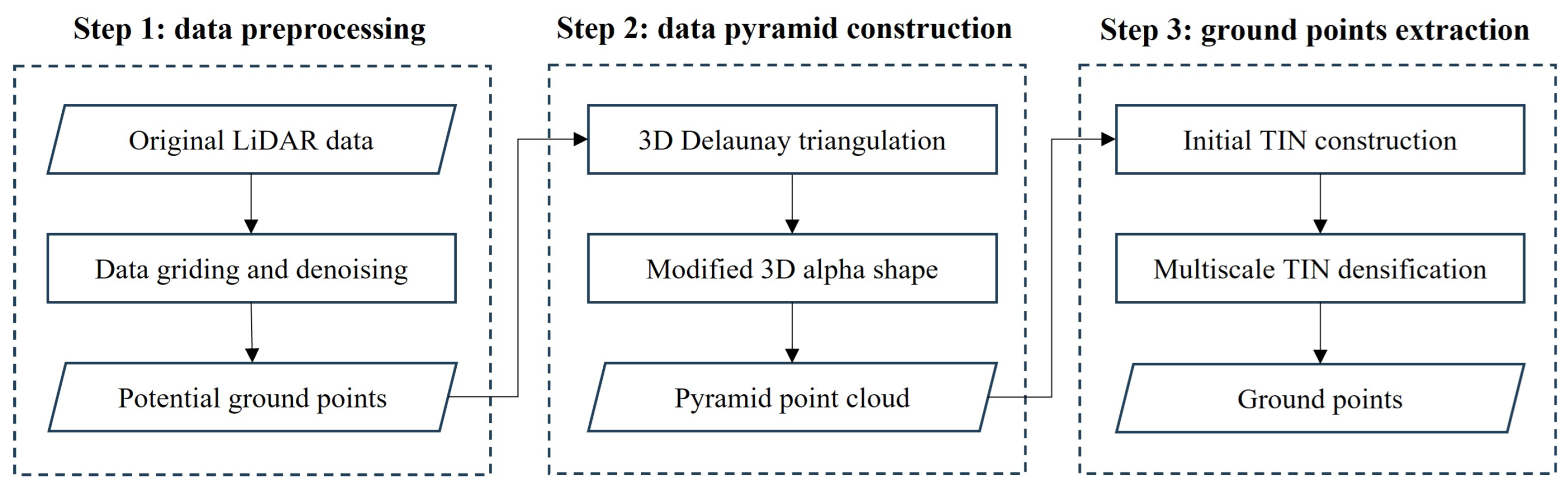
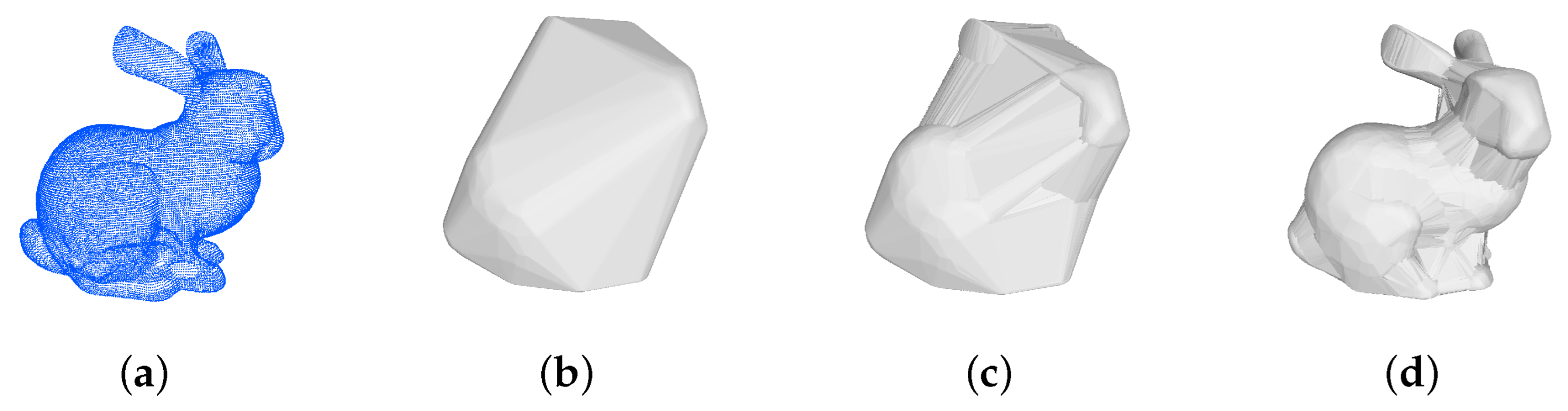
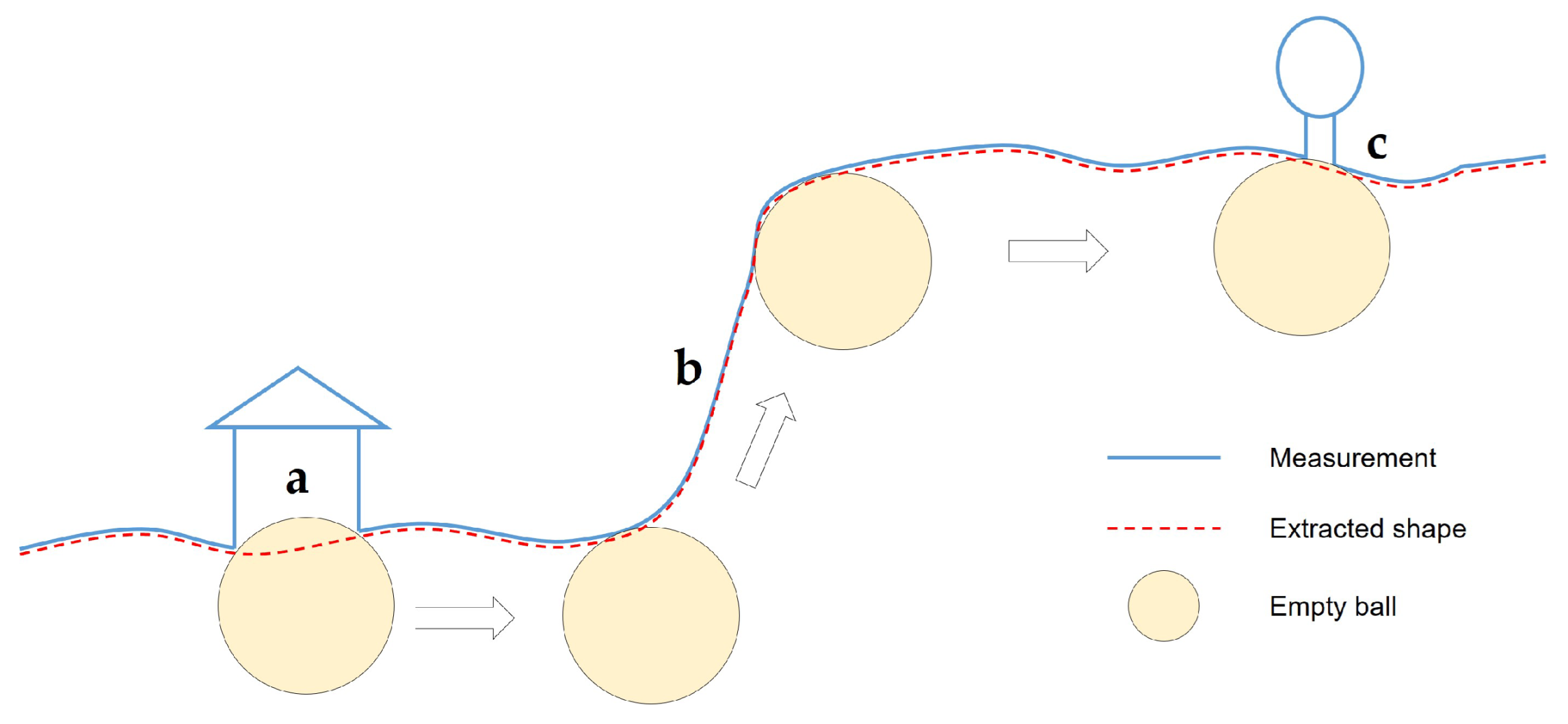
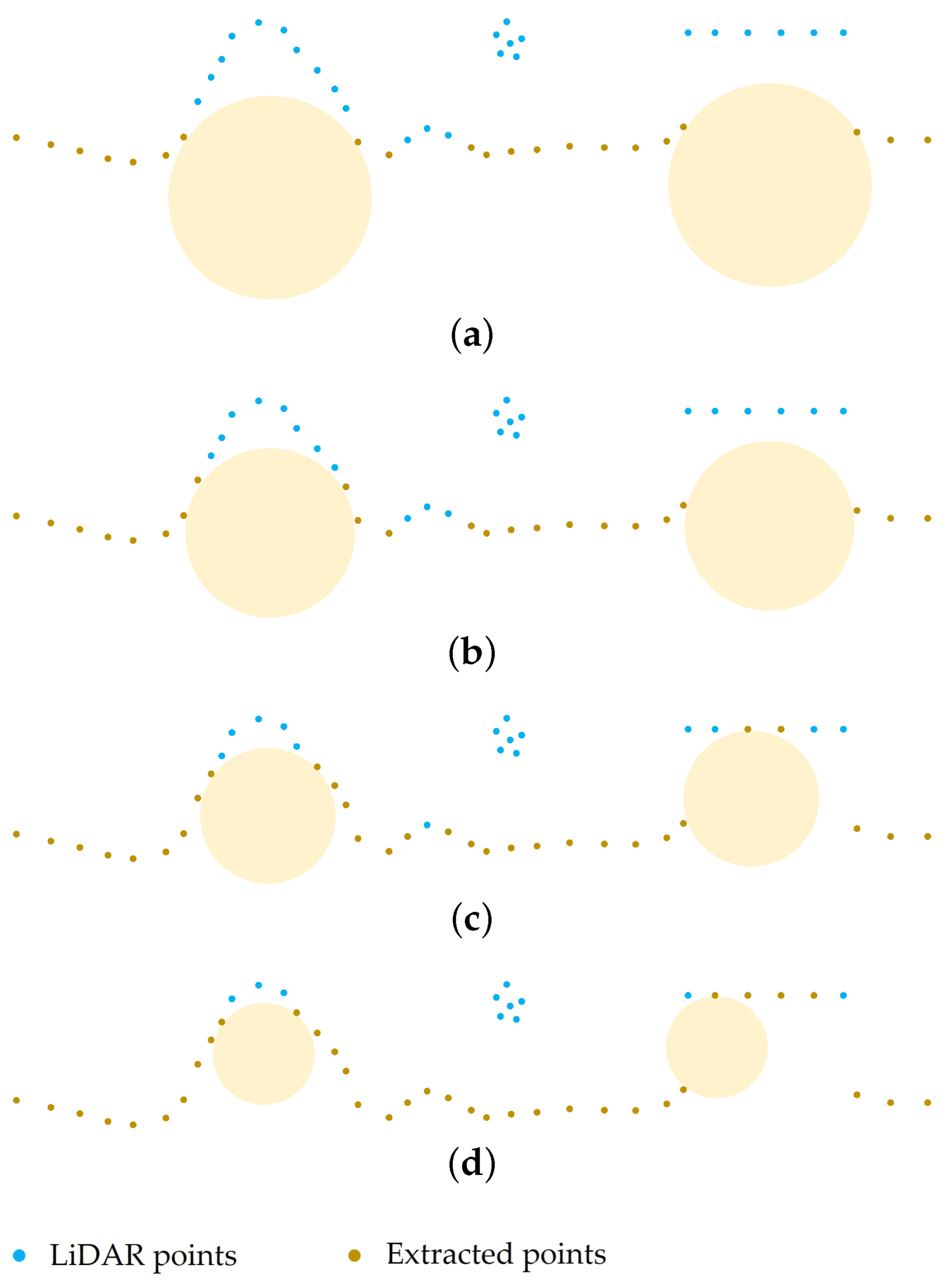
To reliably filter results for complex terrain and steep areas, we developed a filtering method called multiscale alpha shape filtering (MASF). MASF involves three key approaches: in addition to the multiscale comparison strategy and TIN densification mentioned above, the other key approach is the 3D alpha shape algorithm. The alpha shape is widely used to extract the boundary of an unorganized set of points in two or three dimensions [39]. The extraction of geometric boundaries of objects or parts in a point cloud, such as line segments [40] and contours [41], is a fundamental problem in point cloud processing. This allows for more accurate segmentation and surface reconstruction [42]. The 3D alpha shape was first applied for point cloud filtering by Ma et al. 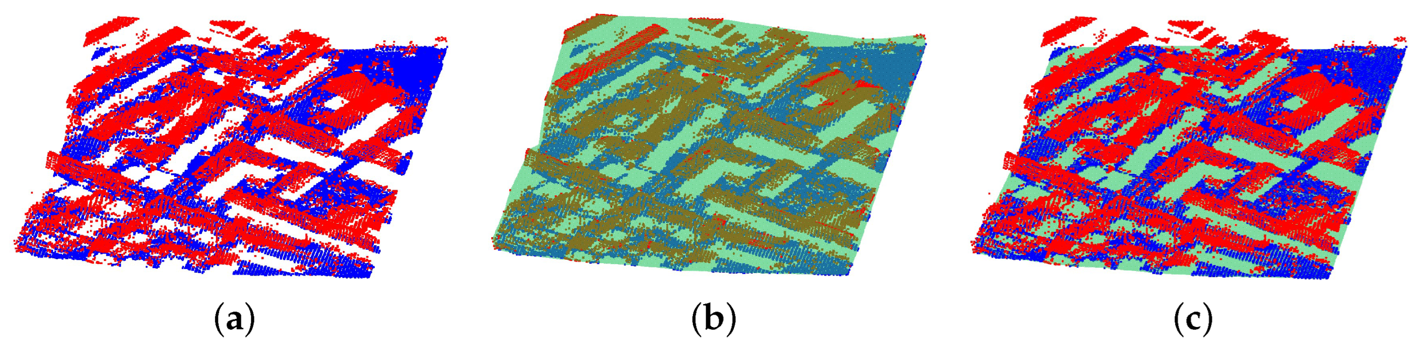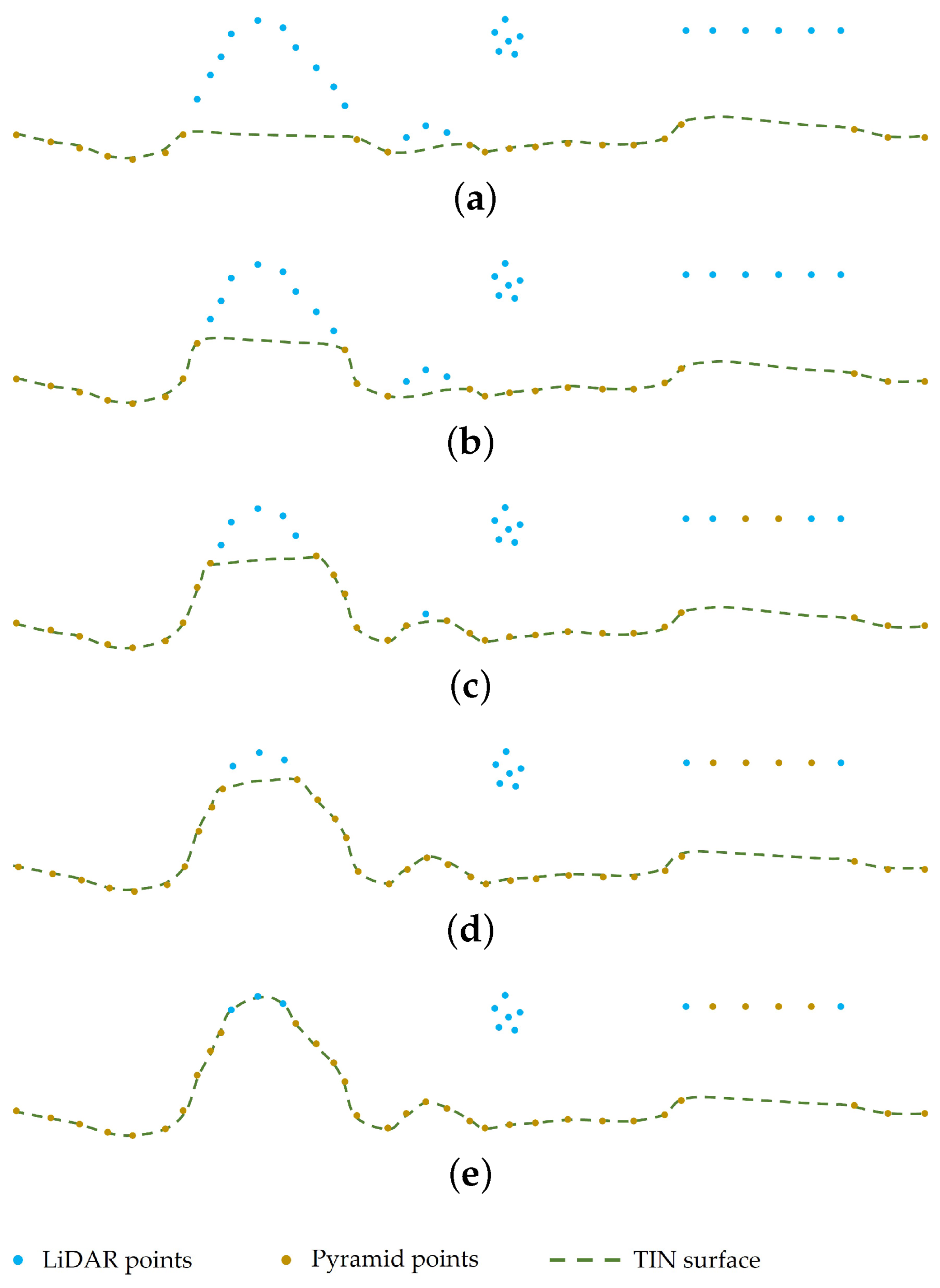by combining the ball pivot algorithm (BPA) and spatial sorting [43]. The nonground points are filtered via an improved BPA traversing all the grids. In this study, we developed a novel application of the 3D alpha shape to filtering. The process of deriving a 3D alpha shape from the underlying Delaunay triangulation is modified by adding extra constraints. A data pyramid consisting of multiscale point layers is constructed using the proposed modified 3D alpha algorithm, and ground points are extracted using top-down multiscale TIN densification.

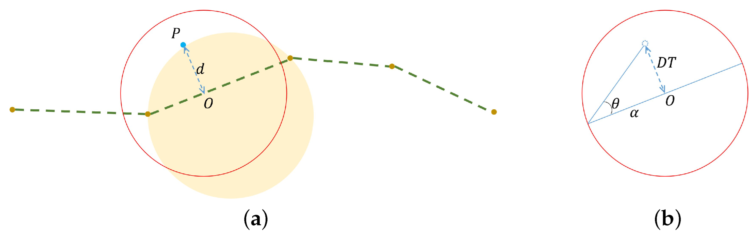
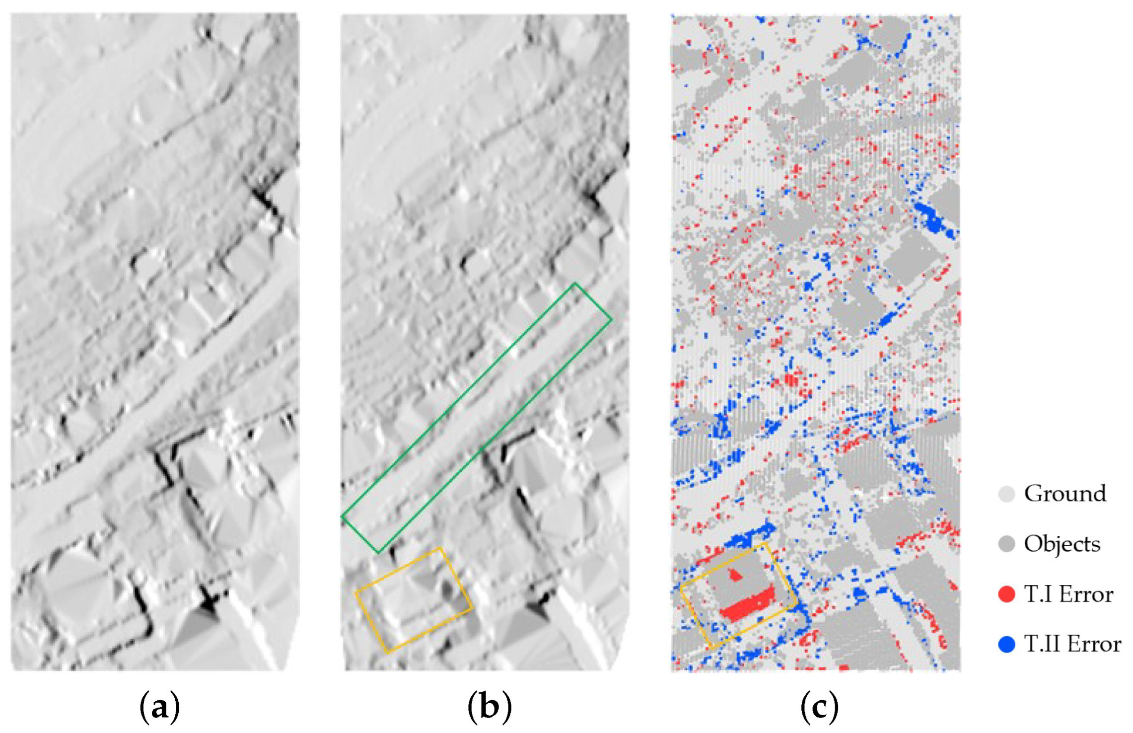
Compared with existing filtering algorithms, the proposed method is innovative in the following two aspects: (1) The data pyramid is built using a novel approach based on the 3D alpha shape. Ground undulations and nonground object points are arranged into point cloud layers at multiple scales based on their size. Compared with using the lowest grid points, this modified 3D alpha shape algorithm is more robust for steep slopes, including cliffs. (2) A multiscale TIN densification approach is used to extract ground points from the pyramid point cloud. The distance thresholds are adaptively determined at each scale, effectively increasing the extraction accuracy in complex scenarios compared with that of classical PTDF. The performance of MASF was quantitatively evaluated using the widely used benchmark dataset provided by the International Society for Photogrammetry and Remote Sensing (ISPRS) commission [15] and an ultra-large-scale ground filtering dataset named OpenGF [44]. The results of the proposed method were compared with those of some classical filtering methods and deep learning pipelines.

The rest of this paper is structured as follows: Section 2 provides a detailed introduction to the proposed method, including the filtering process and parameter determination. Section 3 presents the experimental results and their analysis. Finally, Section 4 discusses the proposed algorithm. The conclusions are summarized in Section 5.

2. Methods

The proposed method uses a multiscale strategy to filter airborne LiDAR data. A novel approach based on the 3D alpha shape is adopted to generate multiscale point cloud layers. The entire workflow of the proposed method consists of three parts, as shown in Figure 1. First, the original data are preprocessed to extract potential ground points without outliers. Second, the data pyramid is generated using the modified 3D alpha shape algorithm with a gradually decreasing $\alpha$. Third, multiscale TIN densification is performed from the top to the bottom layers to extract ground points. A sparse TIN representing the initial ground surface is constructed using the points in the top layer, which solely consists of ground points. In the following layers, the ground points are extracted by examining the point distances from a reconstructed ground surface using an adaptively determined threshold.

2.1. Data Preprocessing

The original LiDAR point cloud contains numerous points, including ground points, nonground points (e.g., buildings, vehicles, and vegetation), and outliers caused by LiDAR system error and multipath reflections [27]. To simplify filtering calcualtion, potential ground points are selected from the original point cloud for further processing. However, negative outliers at low elevations can be erroneously identified as ground points. As a result, the ground points above the outliers are misclassified as nonground points, reducing the filtering accuracy.

To select a set of potential ground points and simultaneously remove negative outliers, the extended local minimum method proposed by Chen et al. [32] is adopted in this method. The input point cloud is initially arranged into a grid G, and each grid cell contains an array of points. For each nonempty cell $G\left(x,y\right)$ in G, a set of low-lying points is selected and sorted via elevation. Starting from the lowest point, if the elevation difference between two adjacent points is smaller than a given threshold, the lower point is selected as a potential ground point. Otherwise, the point is identified as an outlier and removed. The grid is determined by the density of the point cloud. In most cases, a grid size of 1 m is appropriate for the trade-off between terrain detail preservation and grid construction efficiency.

2.2. Modified 3D Alpha Shape

The alpha shape was introduced by Edelsbrunner et al. as a geometric tool to provide reasoning for the shape of an unorganized set of points in 2D, 3D, and higher dimensions [45,46]. An alpha shape is demarcated by a frontier, which is a linear approximation of the original shape [47]. In 3D space, the alpha shape is a computational geometry extension of the point cloud’s convex hull, and each alpha shape is a well-defined polytope. The process of constructing 3D alpha shapes can be intuitively understood as carving the convex hull of the original point set S with an empty ball of user-defined radius $\alpha$. The parameter $\alpha$ determines the desired level of detail (Figure 2). For $\alpha =\infty$, the alpha shape is identical to the convex hull of S. As $\alpha$ decreases, the alpha shape gradually shrinks, degrading to S when $\alpha =0$ [46]. The 3D alpha shape can be derived from the underlying Delaunay triangulation, which is a unique decomposition of the convex hull of a finite set of points S [39]. Each simplex in the triangulation is associated with an interval that specifies the values of $\alpha$ for which the simplex is part of the resulting alpha shape [46].

In this study, the 3D alpha shape was modified to be adaptable to extract the terrain. In the traditional 3D alpha shape algorithm, the triangle ${\sigma }_T$ of the underlying 3D Delaunay triangulation ${\mathcal{Q}}_3$ is part of the resulting shape when the interval specifying the values for which this triangle belongs to the alpha shape contains the user-defined $\alpha$. In our modified version, the triangle must meet two additional conditions: First, the radius of the smallest circumcircle of ${\sigma }_T$ should not be larger than $\alpha$. Second, the triangle must have at least one empty circumscribed sphere with a radius of $\alpha$ located below the bottom of the point cloud. These additional conditions restrict the carving process below the bottom of the input point cloud so that only the bottom points are involved in the calculation (Figure 3). The procedure of the modified 3D alpha shape algorithm is presented in Algorithm 1. The kd tree and TIN constructed with the preprocessed points are used to determine the existence of an empty circumscribed sphere below the bottom of the point cloud. A circumscribed sphere is considered empty if its center contains only three neighbors, which are the vertices of the triangle, within radius $\alpha$. Moreover, a sphere is considered to be below the original point cloud if its center is located beneath the TIN representing the bottom surface.

Because no other points are located below the ground, the extracted bottom frontier of the point cloud can be regarded as the shape that intuitively describes the terrain. The resulting shapes are formed by the triangle of three points, which prevents an empty ball from passing through when the ball rolls under the point cloud. Using an appropriate $\alpha$, the hole of the point cloud under large nonground objects (e.g., buildings and vegetation) prevents the empty ball from passing, and these objects are filtered (see a and c in Figure 4). Furthermore, the points on steep slopes and cliffs can be accurately extracted during ball rolling (see b in Figure 4).

Algorithm 1 The modified 3D alpha shape algorithm.

Require: Preproposed result points $P_l$. Require: Parameter $\alpha >0$; 1: ${\mathcal{Q}}_3\leftarrow$ 3D Delaunay triangulation constructed with $P_l$ 2: ${\mathcal{Q}}_2\leftarrow$ TIN constructed with $P_l$ to determine ball position 3: $T\leftarrow$ kd tree constructed with $P_l$ for searching neighbors in a radius 4: for each triangle ${\sigma }_T$ in ${\mathcal{Q}}_3$ do 5:     $\left[{\alpha }_{min},{\alpha }_{max}\right]\leftarrow$ the interval of ${\sigma }_T$ for specifying the values of $\alpha$ 6:     if $\alpha$∈$\left[{\alpha }_{min},{\alpha }_{max}\right]$ then 7:         Calculate the smallest circumcircle ${\varphi }_T$ of ${\sigma }_T$, and ${\varrho }_T$ is the radius of ${\varphi }_T$ 8:         if ${\varrho }_T=\alpha$ then 9:              $O_T\leftarrow$ the center of ${\varphi }_T$ 10:            Query for neighbors of $O_T$ within radius $\alpha$ in T 11:            if $O_T$ has only three neighbors then          ▹ three vertices of ${\sigma }_T$ 12:                  Label ${\sigma }_T$, and save ${\sigma }_T$ to the final shape ${\mathcal{S}}_{\alpha }$ 13:            end if 14:        else if ${\varrho }_T<\alpha$ then 15:            $B_1$ and $B_2$ ← the circumscribed spheres of ${\sigma }_T$ with a radius of $\alpha$ 16:            $O_1$ and $O_2$ ← the centers of $B_1$ and $B_2$ 17:            Query for neighbors of $O_1$ and $O_2$ within radius $\alpha$ in T, respectively 18:            if either $O_1$ or $O_2$ has only three neighbors and is located under ${\mathcal{Q}}_2$ then 19:                  Label ${\sigma }_T$, and save ${\sigma }_T$ to the final shape ${\mathcal{S}}_{\alpha }$ 20:            end if 21:         end if 22:     end if 23: end for 24: return ${\mathcal{S}}_{\alpha }$

2.3. Data Pyramid Construction

The data pyramid consists of a sequence of point cloud layers that depict the original point cloud at varying scales. Researchers previously constructed the pyramid by selecting the lowest points of the grid cells and adjusting the scale by changing the cell size [13,32]. However, this approach encounters difficulties in extracting evenly distributed representative points on steep slopes and cliffs. Instead, we used the modified 3D alpha shape algorithm to address these issues. Figure 5 illustrates the extraction of point cloud layers using a series of gradually decreasing $\alpha$ values. For the top layer, a sufficiently large parameter denoted by ${\alpha }_{max}$ is used to extract a shape that roughly represents the ground surface, consisting solely of ground points. According to the prior knowledge that the surface is continuous, the closer the two ground points, the smaller their elevation difference. Conversely, nonground points may cause sudden a relief change across a short horizontal distance [27]. As $\alpha$ decreases, the slopes are extracted from the base to the top, whereas the buildings are extracted in the opposite direction (Figure 5). The difference in elevation between the adjacent layers of ground points is small, whereas that between object points and ground points is large, allowing ground and nonground points to be distinguished by analyzing their distance to a reconstructed ground surface.

During the construction of the data pyramid, $\alpha$ linearly decreases from ${\alpha }_{max}$ to ${\alpha }_{min}$ in steps of ${\alpha }_{step}$. This linearly decreasing $\alpha$ preserves the gradually changing topographic features. The value of $\alpha$ for each layer, from top to bottom, can be calculated using the following formula:

$${\alpha }_k={\alpha }_{max}-(k-1)\times {\alpha }_{step}$$

(1)

where $k=1,2,\dots ,M$. The value of ${\alpha }_{max}$ is determined from the size of the largest nonground object in the original point cloud. ${\alpha }_{max}$ should be sufficiently large to filter all noground points in the top layer. In practice, ${\alpha }_{max}$ is usually set to half the size of the largest object. However, when large-scale buildings exist, ${\alpha }_{max}$ should be further increased to be larger than the largest object size due to the curvature of the empty ball. Typically, ${\alpha }_{min}$ is twice the grid size used in the preprocessing, because the density of the preprocessed point cloud is determined using the grid size. ${\alpha }_{step}$ determines the number of layers in the data pyramid. A smaller ${\alpha }_{step}$ leads to more gradual changes between layers and helps to preserve terrain details. However, a smaller ${\alpha }_{step}$ also requires more computation. A further analysis of the setting of ${\alpha }_{step}$ is discussed in Section 4.2.

2.4. Multiscale TIN Densification Filter

The classical PTDF proposed by Axelsson et al. [2] is an iterative process. An unclassified point is identified as a ground point and added to the TIN if its iterative angle and distance from the TIN face are smaller than the corresponding user-defined thresholds [28]. In this paper, a multiscale TIN densification approach is developed to extract ground points. Compared with the classical PTDF, multiscale TIN densification provides three aspects of improvements. First, the initial sparse TIN is constructed using points extracted using the modified 3D alpha shape algorithm, which provides a larger number and a more even distribution than using the lowest points of the grid cells in PTDF (further comparisons are provided in Section 4.1). Second, only the distance threshold is needed to identify the ground points, whereas two user-defined thresholds need to be examined with the classical PTDF. Moreover, the distance threshold can be adaptively determined in each layer. Third, multiscale TIN densification is a noniterative process, and ground points are only identified once in each layer, considerably simplifying the computation process.

The multiscale TIN densification procedure is illustrated in Figure 6. TIN densification is accomplished using point cloud layers in the data pyramid in a top-down approach. The points in the top layer are used as seeds to build a sparse TIN that represents the initial ground surface (Figure 6a). The quality of the TIN at the edge is low due to the lack of neighboring points. The credibility of long narrow triangles and vertical triangles is low, which may lead to the misclassification of nonground points at the edges. To solve this problem, empty cells are added around the grid established during preprocessing to create buffer zones that expand the data processing region. The centers of these empty cells are then used as simulated ground points, with their elevation set to that of the nearest point in the top layer. This technique helps with eliminating edge effects and preventing the formation of low-credibility long and narrow triangles along the boundary [28]. In the subsequent layers, points closer to TIN than the corresponding distance threshold ($DT$) are labeled as ground points and inserted into the TIN, resulting in a further refined surface with more terrain details. However, some ground points remain in the original point set due to potential ground point selection in preprocessing and omissions during TIN densification. Thus, the distances between all unlabeled points and the TIN are computed to completely extract ground points. Those with distances less than the final threshold ($FT$) are added to the final ground point set (Figure 6e).

In this approach, the determination of the $DT$ used in each layer is crucial. The residuals of ground points to the TIN, which represents the ground surface, are larger than those of nonground objects. Therefore, ground and nonground points can be differentiated using an appropriate $DT$. In the starting layers, $DT$ should be large enough to recover as much as possible of the terrain, because the initial surface is rough. However, for subsequent layers, $DT$ should gradually decrease to avoid misclassifying small nonground objects that are attached to the ground. As illustrated in Figure 7a, the distance d between the point P and its nearest TIN facet is calculated when detecting whether P is a ground point. Suppose that a ball exists with radius $\alpha$ centered on O, which is the perpendicular foot of P to the nearest facet. $\theta$ is the relative slope that determines the value of $DT$. The distance threshold denoted by $D{T}_k$ in the kth layer can be derived from the corresponding ${\alpha }_k$ using the following formula:

$$D{T}_k=ST{\alpha }_k+FT$$

(2)

where $k=1,2,\dots ,M$. $ST$ refers to the slope threshold: a user-defined parameter equivalent to tan$\theta$. For simplification, $ST$ is typically set to 0.01 (tan3°) in flat areas and 0.1 (tan6°) in areas with relief. For steep slopes, $ST$ can be even larger to extract points on ridges and cliff edges. $FT$ is mainly used to determine the threshold in the bottom layers, because the corresponding $\alpha$ decreases to a small value. In practice, $FT$ is usually set to 0.5 m to balance the removal of nonground objects attached to the ground and the preservation of minor terrain details.

3. Experiment and Results

3.1. Experimental Setup

The proposed method was implemented in C++ and compiled using Visual Studio 2017. The algorithms provided by the Computational Geometry Algorithm Library (CGAL) were employed to construct the Delaunay triangulation and calculate the corresponding interval for each simplex [48]. CGAL is an open-source software project that provides access to geometric algorithms in the form of a C++ library. For point sets in two or three dimensions, CGAL offers packages that enable the construction and manipulation of Delaunay triangulations. Triangulations can be incrementally constructed and efficiently modified by inserting, displacing, or removing vertices. The experiments were conducted using a desktop computer with an Intel Core i9-9900K CPU @3.60 GHz and 32 GB RAM (HP, Palo Alto, CA, USA).

3.2. Accuracy Metrics

We used four accuracy metrics derived from the error matrix of the filtering results (see

Table 1. Error matrix of the filtering results.

		Filtered
		Ground Points	Nonground Points
Reference	Ground points	a	b
	Nonground points	c	d

) and used in prior studies to evaluate the performance of the proposed method. The type I error (T.I), type II error (T.II), total error (T.E.), and kappa coefficient ($\kappa$) were calculated and compared with those of some current top algorithms. Type I error (Equation (3)) is the percentage of ground points misclassified as nonground points, and type II error (Equation (4)) is the proportion of nonground points classified as ground points. The total error (Equation (5)) is the overall proportion of incorrectly classified points. The kappa coefficient (Equation (6)) is an alternative measure of the overall classification accuracy in which the effect of chance agreement is subtracted, and the increase in the accuracy of a particular classification is quantified compared with that of a random classification [49].

$$TypeIerror=\frac{b}{a+b}$$

(3)

$$TypeIIerror=\frac{c}{c+d}$$

(4)

$$Totalerror=\frac{b+c}{a+b+c+d}$$

(5)

$$Kappacoefficient=\frac{p_0-p_c}{1-p_c}$$

(6)

where $e=a+b+c+d$, $p_0=\frac{\left(a+d\right)}{e}$ and $p_c=\frac{\left(a+b\right)\times \left(a+c\right)+\left(c+d\right)\times \left(b+d\right)}{e^2}$.

3.3. Testing Results

3.3.1. Testing with ISPRS Dataset

We employed the benchmark datasets provided by the International Society for Photogrammetry and Remote Sensing (ISPRS) Working Group III/3 to test the performance of our method in various scenarios [15]. The dataset comprises 15 samples from seven sites, encompassing a variety of feature objects such as vegetation, buildings, roads, railroads, rivers, bridges, power lines, and water surfaces. The samples were captured with an Optech ALTM scanner, and the average point spacing is 1.0–1.5 m in urban areas (from samp11 to samp42) and 2.0–3.5 m in rural areas (from samp51 to samp71).

Table 2. Features of the samples in the ISPRS dataset [15,24].

Environment	Site	Sample	Features
Urban	1	11	Mixture of vegetation and buildings on the hillside
		12	Mixed vegetation and buildings
	2	21	Large buildings and bridge
		22	Irregularly shaped buildings
		23	Large, irregularly shaped buildings
		24	Steep slopes with vegetation
	3	31	Complex buildings
	4	41	Data gaps, vegetation on moderate slopes
		42	Railway station with trains
Rural	5	51	Gaps, vegetation on moderate slopes
		52	Large buildings and bridge
		53	Irregularly shaped buildings
		54	Large, irregularly shaped buildings
	6	61	Steep slopes and large gap
	7	71	Steep slopes and bridge.

shows the detailed features of each sample. The reference filtering result for each sample was obtained via semiautomatic filtering and manual editing using knowledge of the landscape [15].

Table 3. Performance evaluations of MASF on the dataset provided by the ISPRS and the corresponding parameters.

Sample	Parameter			Result
	${\mathit{\alpha }}_{\mathit{max}}$ (m)	${\mathit{\alpha }}_{\mathit{step}}$ (m)	ST	T.I (%)	T.II (%)	T.E. (%)	kappa (%)
samp11	28	1	0.10	6.60	11.59	8.73	82.10
samp12	25	1	0.05	2.50	3.94	3.20	93.60
samp21	20	2	0.05	0.49	3.48	1.15	96.65
samp22	25	1	0.10	2.79	8.67	4.61	89.16
samp23	15	1	0.10	1.75	9.80	5.56	88.80
samp24	10	1	0.10	4.10	13.12	6.58	83.37
samp31	25	2	0.01	0.90	1.87	1.35	97.28
samp41	25	2	0.05	5.11	1.78	3.45	93.09
samp42	20	9	0.10	0.99	0.80	0.85	97.95
samp51	25	4	0.05	0.34	5.52	1.47	95.61
samp52	20	1	0.05	3.10	17.02	4.57	76.70
samp53	7	1	0.25	0.99	39.45	2.54	64.49
samp54	20	9	0.05	2.46	3.16	2.84	94.30
samp61	6	1	0.10	0.33	12.02	0.73	88.82
samp71	15	2	0.05	0.94	5.70	1.48	92.66
Avg.				2.23	9.19	3.27	88.97

presents the parameters and results of the proposed method for 15 sample types. For each sample, the parameters were tuned according to the features of the scene. The three main user-defined parameters in MASF are ${\alpha }_{max}$ and ${\alpha }_{step}$ for the construction of pyramid point clouds and $ST$ for the determination of the distance threshold in each iteration. ${\alpha }_{max}$ varies from 5 to 25 m, depending on the largest nonground object in the sample. In particular, the ${\alpha }_{max}$ for smap42 was set to 20 m due to the extremely large size of the train station building, whereas the $\alpha$ in the top layer was set to 90 m to avoid unnecessary computation.

Table 3 shows that the overall average total error and kappa coefficient of MASF were 3.27% and 88.97%, respectively. MASF performed relatively well for samp21, samp31, samp42, samp51, samp53, samp54, samp61, and samp71 in terms of both total error and kappa coefficient. These samples contain a variety of features, indicating that MASF is highly accurate in scenarios with various objects and slopes. The total errors for samp11, samp12, samp22, samp23, samp24, samp41, and samp52 were relatively higher than those for the other samples, which could have been a result of terraced slopes (e.g., riverbanks, ditches, and terraces) in these samples. Because terraced slopes are more frequent in artificial scenarios, MASF performed better in rural areas than in urban areas, with an average total error of 2.27% in rural areas and 3.94% in urban areas.

Regarding individual sample accuracy, the total error was highest for samp11, which contained a complex configuration of steep slopes, buildings, and low vegetation. The type I error of samp11 was also the highest due to the mixing of complex features. The kappa coefficient and type II error for samp53 were the worst, which were a result of the low number of nonground points in this sample. A small amount of low vegetation was misclassified, resulting in a notable rise in the kappa coefficient. An abnormally small kappa coefficient for samp53 was also obtained with the other filtering methods. However, MASF achieved one of the highest kappa coefficient among the considered methods.

MASF exhibited a bias toward type II errors, with a substantially larger average type II error than type I error for most samples. The reason for this tendency may be the surface recovery strategy employed in our method and the imbalance in the number of ground and nonground points. Many small terrain features (e.g., protrusions and edges) were misclassified as nonground points due to the failure to recover terrain details during the filtering process, leading to larger type II errors. However, the bias toward type II errors may not be a disadvantage of the proposed method, as type II errors can be more easily handled via manual postprocessing editing than type I errors [13].

To qualitatively analyze the performance of MASF for various scenarios, we selected one representative sample from each of the seven sites in the dataset. The results on the four samples selected in urban areas, including samp11, samp22, samp31, and samp42, are shown in Figure 8, Figure 9, Figure 10 and Figure 11. The three samples selected from rural areas were samp53, samp61, and samp71; their results are shown in Figure 12, Figure 13 and Figure 14. As shown in these figures, artificial objects, such as buildings and bridges, were effectively filtered. In terms of error distribution, type II errors mainly arose along the edges of terraced floors, whereas type I errors were mainly associated with low vegetation attached to the ground.

For comparison with previous filters, we selected eight methods, seven of which were representative of those proposed in recent years, as well as Axelsson’s PTDF, which performed the best in an experimental comparison conducted by Sihole and Vosselman in 2004 [15].

Table 4. Error comparison among algorithms for dataset provided by the ISPRS (%).

Sample	Axelsson (2000)	Mongus (2012)	Chen (2013)	Pingel (2013)	Hu (2014)	Mongus (2014)	Hui (2016)	Zhang (2016)	MASF
samp11	10.76	11.01	13.01	8.28	8.31	7.50	13.34	12.01	8.73
samp12	3.25	5.17	3.38	2.92	2.58	2.55	3.50	2.97	3.20
samp21	4.25	1.98	1.34	1.10	0.95	1.23	2.21	3.42	1.15
samp22	3.63	6.56	4.67	3.35	3.23	2.83	5.41	8.94	4.61
samp23	4.00	5.83	5.24	4.61	4.42	4.34	5.11	4.79	5.56
samp24	4.42	7.98	6.29	3.52	3.80	3.58	7.47	2.87	6.58
samp31	4.78	3.34	1.11	0.91	0.90	0.97	1.33	1.61	1.35
samp41	13.91	3.71	5.58	5.91	5.91	3.18	10.60	5.14	3.45
samp42	1.62	5.72	1.72	1.48	0.73	1.35	1.92	1.58	0.85
samp51	2.72	2.59	1.64	1.43	2.04	2.73	4.88	3.08	1.47
samp52	3.07	7.11	4.18	3.82	2.52	3.11	6.56	3.93	4.57
samp53	8.91	8.52	7.29	2.43	2.74	2.19	7.47	5.20	2.54
samp54	3.23	6.73	3.09	2.27	2.35	2.16	4.16	3.18	2.84
samp61	2.08	4.85	1.81	0.86	0.84	0.96	2.33	1.49	0.73
samp71	1.63	3.14	1.33	1.65	1.50	2.49	3.73	5.71	1.48
Avg.	4.82	5.62	4.11	2.97	2.85	2.74	5.33	4.39	3.27

The bolded numbers are the lowset total error in each sample.

and

Table 5. Kappa coefficient comparison among algorithms for dataset provided by the ISPRS (%).

Samples	Axelsson (2000)	Chen (2013)	Pingel (2013)	Hu (2014)	Hui (2016)	Zhang (2016)	MASF
samp11	78.48	74.12	83.12	82.97	72.92	75.17	82.10
samp12	93.51	93.23	94.15	94.83	93.00	94.04	93.60
samp21	86.34	96.10	96.77	97.23	93.35	90.47	96.65
samp22	91.33	89.03	92.21	92.04	87.58	77.72	89.16
samp23	91.97	89.49	90.73	91.14	89.74	90.38	88.80
samp24	88.50	84.53	91.13	90.39	81.93	92.68	83.37
samp31	90.43	97.76	98.17	98.19	97.33	96.75	97.28
samp41	72.21	88.83	88.18	88.18	78.78	89.73	93.09
samp42	96.15	95.81	96.48	98.25	95.38	96.18	97.95
samp51	91.68	95.17	95.76	93.90	85.06	91.13	95.61
samp52	83.63	78.91	81.04	86.24	69.51	77.05	76.70
samp53	39.13	46.69	68.12	66.43	41.84	46.86	64.49
samp54	93.52	93.90	95.44	95.28	91.63	93.61	94.30
samp61	74.52	77.36	87.22	86.76	67.82	78.10	88.82
samp71	91.44	93.19	91.81	92.59	79.86	68.03	92.66
Avg.	84.19	86.27	90.02	90.29	81.72	83.86	88.97

The bolded numbers are the highest kappa coefficient in each sample.

summarize the total errors and kappa coefficients for these methods and MASF. In most samples, MASF almost achieved higher accuracy and the lowest total error for samp61. In general, our method demonstrates accuracy comparable to that of the top filtering algorithms.

3.3.2. Testing with OpenGF Dataset

To evaluate the performance of MASF for large scenes, a large-scale and scene-rich ground filtering dataset called OpenGF (https://github.com/Nathan-UW/OpenGF (accessed on 1 March 2024)) was adopted for testing [34,44]. This dataset was built upon open airborne LiDAR data from around the world, covering over 47 km² of 9 different typical terrain scenes in 4 different countries. The points in this dataset have high-quality labels as ground, nonground, and outliers. OpenGF offers a challenging test set consisting of Test I, Test II, and Test III, covering a wide range of spatial areas and diverse terrain types. Test I includes a mixed area with a village, small city, and mountain. Test II involves metropolitan areas and contains various objects of different sizes, such as large and small roofs, cars, and grass. Please note that numerous high and low outliers in Test II were removed before testing with MASF because MASF cannot process data with normally distributed dense outliers. Test III is characterized by extremely sparse ground points under dense vegetation and terraced slopes with sharply changing elevations. Four classic ground filters (PTDF [2], PMF [20], MCC [50], and CSF [20]) and four state-of-the-art 3D DNNs (PointNet++ [35], KPconv [36], RandLA-Net [37], and SCF-Net [38]) were tested, and the results were released by Qin et al. [34]. Specifically, the intersection over the union ($IoU$) of each class was computed to elevate the class-wise precision. $Io{U}_1$ (Equation (7)) and $Io{U}_2$ (Equation (8)) are the $IoU$ of the ground (class 1) and nonground (class 2) points, respectively.

$$Io{U}_1=\frac{TP}{TP+FP+FN}$$

(7)

$$Io{U}_2=\frac{TN}{TN+FN+FP}$$

(8)

where TP, FP, TN, and FN denote the number of correctly identified ground points, the number of ground points incorrectly identified as nonground points, the number of correctly identified nonground points, and the number of nonground points incorrectly identified as ground points, respectively.

Table 6. Accuracy comparison of algorithms on OpenGF dataset (%).

	Test I			Test II (w/o Outliers)			Test III
	TE (%)	IoU1 (%)	IoU2 (%)	T.E. (%)	IoU1 (%)	IoU2 (%)	T.E. (%)	IoU1 (%)	IoU2 (%)
MASF	2.34	94.85	95.88	3.92	92.59	92.31	1.94	89.87	97.66
PTDF	5.18	89.00	91.10	6.70	87.24	87.64	2.45	87.16	97.05
PMF	8.37	79.62	85.22	13.44	73.61	78.50	5.07	73.67	94.09
MCC	3.71	91.86	93.63	15.56	70.27	75.39	3.03	84.12	96.40
CSF	6.93	85.64	88.17	10.66	80.38	81.08	4.65	78.29	94.42
PointNet++	2.42	94.68	95.75	12.62	79.63	75.19	1.88	90.24	97.72
KPConv	2.21	95.17	96.10	8.91	84.67	82.44	1.69	91.28	97.94
RandLA-Net	3.71	91.65	93.74	5.04	90.42	90.38	2.40	87.08	97.14
SCF-Net	4.25	90.43	92.90	9.09	83.32	83.35	2.77	85.18	96.70

The bolded numbers are the highest accuracy achieved by classic and learning-based methods in each sample, respectively.

presents the accuracy of the results of the proposed method with that of the eight other methods. The accuracy of MASF was the highest on all three test samples among the classic filter methods. Additionally, MASF outperformed most learning-based approaches. Figure 15 provides the qualitative evaluation of the filtering results obtained with MASF on the three samples. In Test I, MASF successfully filtered vegetation and forests. The errors in the result were primarily caused by the omission of ground points on the mountain ridges. MASF outperformed all learning-based pipelines on Test II due to its ability to handle large buildings. Buildings that posed challenges for learning-based pipelines were successfully removed with MASF. In Test III, the ground points on slopes with sharply changing elevations were correctly extracted. The misclassified points mainly arose in low vegetation due to the lack of ground points under dense forests. In general, MASF robustly and stably performed in large-scale scenes with complex terrain features and diverse objects.

3.4. Algorithm Efficiency Comparison

To assess the efficiency of the proposed method, we measured the computation time of MASF and two open-source filtering methods (PMF and CSF) during testing on the ISPRS dataset. Progressive morphological filtering (PMF) is a morphology-based method and is available for open access in the Point Cloud Library (https://pointclouds.org/ (accessed on 1 April 2024, v1.14.0)). Cloth simulation filtering (CSF) is a surface-based filtering method that was open-sourced by the authors, which was implemented in C++ and released on GitHub (https://github.com/jianboqi/CSF (accessed on 1 April 2024)).

When testing on the ISPRS dataset, the cell size of the grid construction in three filtering methods was all set to 1 m. The maximum iterations of CSF were set to 1000, and postprocessing was enabled. Other parameters were tuned based on the sites. Figure 16 shows the calculation times of the three methods. MASF, CSF, and PMF had average calculation times of 2.44, 3.53, and 0.59 s, respectively. When testing on the OpenGF dataset, the approximate computation time reported by Qin et al. was used for comparisons, because we used the same hardware [34]. The approximate calculation time of MASF and the six selected methods are presented in

Table 7. Approximate calculation time (minutes) of MASF and six selected methods on the OpenGF dataset.

	Test I	Test II (w/o Outliers)	Test III
MASF	27.1	6.3	7.08
PTD	2.8	0.2	0.8
PMF	0.7	1.5	0.4
CSF	14.6	0.7	7.8
KPConv	2.3	0.2	1.3
RandLA-Net	1.9	0.3	1.2
SCF-Net	2.1	0.3	1.2

. The results indicated that the efficiency of the proposed method was acceptable when filtering relatively small data. MASF was comparable to CSF in efficiency but was less efficient than PMF. However, MASF was time-consuming when dealing with large-scale data. The calculation time of MASF was heavily influenced by the number of points. As the number of points increased, the number of triangles that needed to be evaluated in the underlying triangulation rapidly increased. Because the judgments on each triangle are independent of each other, parallel computing can be employed to accelerate the modified 3D alpha-shape algorithm in the future.

4. Discussion

4.1. Accuracy of Ground Seeds

In previous studies, ground seeds have usually been obtained by selecting the lowest point within each cell of a gird [27]. To ensure that there are no non-ground points among the seeds, the cell size ($CS$) must be larger than that of the largest nonground object (e.g., building) in the point cloud. The number of seeds is equal to the number of nonempty cells, which is too small to approximate the terrain well.

This paper presented a novel approach for extracting ground seeds using a modified 3D alpha shape algorithm. To evaluate the effectiveness of this approach, we selected two representative samples from the ISPRS dataset and compared the results with those obtained using two different methods. Figure 17 shows that the ground seeds extracted with our method can more comprehensively cover terrain features. The lowest points of the grid cells are primarily located at the base of these slopes in areas with steep slopes, causing the omission of points on cliffs and abrupt slopes. In contrast, our method can extract seeds on various slopes, including those on cliffs (Figure 17e). The ground surface constructed using these seeds relatively accurately captures the terrain details, especially on steep slopes.

To quantitatively assess the accuracy of the extracted ground seeds, we separately applied the approach using the lowest point of the grid cells and the modified 3D alpha shape algorithm to the 15 samples. The numbers of extracted seeds are listed in

Table 8. Number and overall precision of ground seeds.

Sample	Lowest Cell			Ours
	CS (m)	Points	OP (%)	${\mathit{\alpha }}_{\mathit{max}}$ (m)	Points	OP (%)
samp11	20	112	99.11	28	4166	99.26
samp12	20	154	94.81	25	12,622	99.60
samp21	25	25	100.00	20	5420	99.83
samp22	40	25	100.00	25	9242	99.83
samp23	25	54	100.00	15	6923	98.07
samp24	15	45	100.00	10	3068	98.57
samp31	25	49	93.88	25	9147	99.63
samp41	25	35	94.29	25	2150	99.81
samp42	30	25	100.00	20	3631	99.75
samp51	20	264	98.48	25	13,043	99.42
samp52	10	1325	98.26	20	15,206	99.60
samp53	10	1937	99.79	7	31,290	99.42
samp54	15	234	99.15	20	3731	98.25
samp61	15	870	99.88	6	33,536	99.59
samp71	20	221	99.55	15	12,471	99.79

. Additionally, the overall precision ($OP$) was employed to evaluate the quality of the ground seeds obtained with this method, which is the correct classified ground seeds for all the ground seeds extracted. Table 8 shows that our method highly accurately extracted ground seeds, with an average overall precision of 99.36% on the 15 samples. Our method also extracted substantially more seeds than that obtained using the lowest cell point.

In summary, our method can extract more points and obtain a more even point distribution than using the lowest points of the grid cells. Selecting ground seeds to represent the ground is a strategy commonly employed in many filtering methods. High-quality seeds have a strong positive impact on point cloud filtering. Our method offers a new approach to extracting ground seeds and has the potential to increase the precision of filters that need initial seeds.

4.2. Analysis of Parameter Settings

The filtering accuracy of MASF is strongly impacted by the parameter $\alpha$ of the modified 3D alpha shape algorithm. As such, we analyzed the selection of $\alpha$ in each iteration. $\alpha$ determines the scale of the corresponding point layer generated with the modified 3D alpha shape algorithm. $\alpha$ linearly decreases from ${\alpha }_{max}$ to ${\alpha }_{min}$ in steps of ${\alpha }_{step}$. Setting ${\alpha }_{step}$ properly is crucial in the proposed method because the value of ${\alpha }_{max}$ is determined using the largest nonground object in the point cloud.

To quantitatively assess the influence of ${\alpha }_{step}$ on filtering accuracy, we tested all 15 samples from the ISPRS benchmark dataset using ${\alpha }_{step}$, which ranged from 1 to 9 m in 1 m steps. All other parameters were kept the same as those used in the experiments described in Section 3. The total errors for each sample, which depend on ${\alpha }_{step}$, are illustrated in Figure 18. The samples were divided into urban and rural groups according to their sites. The mean total errors for both groups and all samples were separately calculated, with the results shown in Figure 18c. In general, the total error increased as ${\alpha }_{step}$ increased, and the accuracy was highest for most samples when ${\alpha }_{step}$ was 1 or 2 m. Furthermore, the standard deviations of the total errors were calculated for each sample to evaluate the sensitivity of the total errors with respect to ${\alpha }_{step}$ (Figure 18d). Figure 18d indicates that the samples with steep slopes (e.g., smap11, samp52, and samp53) and terraced floors (e.g., samp23 and samp24) were more sensitive to the increase in ${\alpha }_{step}$. When ${\alpha }_{step}$ is large, the proposed method may struggle to recover terrain details due to the limited number of iterations in complex scenarios. This could result in the loss of terrain relief and the truncation of terraced floors, leading to larger type II and total errors.

5. Conclusions

In this paper, a new method is presented for filtering airborne LiDAR point clouds, called multiscale alpha shape filtering (MASF). In MASF, a multiscale strategy is used to reconstruct the ground surface by incorporating the ground points extracted at different scales. A novel approach based on 3D alpha shapes is used to construct a data pyramid. The scales of the point cloud layers are adjusted by changing the parameter $\alpha$. Ground points are extracted from the data pyramid in a top-to-bottom approach using a multiscale TIN densification method. The points in the top layer are used as ground seeds to construct the initial TIN. An adaptively determined distance threshold is used to identify ground points in each layer. The proposed method was tested on a benchmark dataset provided by ISPRS and a large-scale dataset called OpenGF. The performance of the proposed MASF algorithm showed promise compared with that of existing methods. The average total error and the kappa coefficient on the ISPRS dataset were 3.27% and 88.97%, respectively.

However, the MASF has a limitation: for terrain with terraced slopes such as riverbanks, ditches, and terraces, extracting the edges of terraced floors can be challenging. This can result in the omission of ground points. To increase the adaptability of MASF, segmentation and classification techniques can be considered to extract complete ground points in future studies. Terraced floor points can be preclustered into their own segments to ensure surface completeness. Moreover, MASF can be time-consuming when dealing with scenarios involving complex objects on slopes. To increase efficiency, parallel computing can be applied to generate point cloud layers in the future.

References

1. Kraus, K.; Pfeifer, N. Determination of terrain models in wooded areas with airborne laser scanner data. ISPRS J. Photogramm. Remote Sens. 1998, 53, 193–203. [Google Scholar] [CrossRef]
2. Axelsson, P. DEM Generation from Laser Scanner Data Using adaptive TIN Models. Int. Arch. Photogramm. Remote Sens. 2000, 23, 110–117. [Google Scholar]
3. Wang, C.; Tseng, Y. DEM gemeration from airborne lidar data by an adaptive dualdirectional slope filter. Int. Arch. Photogramm. Remote Sens. Spat. Inf. Sci.-Arch. 2010, 38, 628–632. [Google Scholar]
4. Susaki, J. Adaptive Slope Filtering of Airborne LiDAR Data in Urban Areas for Digital Terrain Model (DTM) Generation. Remote Sens. 2012, 4, 1804–1819. [Google Scholar] [CrossRef]
5. Mongus, D.; Zalik, B. Parameter-free ground filtering of LiDAR data for automatic DTM generation. ISPRS J. Photogramm. Remote Sens. 2012, 67, 1–12. [Google Scholar] [CrossRef]
6. Zhang, J.; Hu, X.; Hengming, D.; Qu, S. DEM Extraction from ALS Point Clouds in Forest Areas via Graph Convolution Network. Remote Sens. 2020, 12, 178. [Google Scholar] [CrossRef]
7. Krisanski, S.; Taskhiri, M.S.; Gonzalez Aracil, S.; Herries, D.; Muneri, A.; Gurung, M.B.; Montgomery, J.; Turner, P. Forest Structural Complexity Tool—An Open Source, Fully-Automated Tool for Measuring Forest Point Clouds. Remote Sens. 2021, 13, 4677. [Google Scholar] [CrossRef]
8. Wang, P.; Cao, D.; Xia, S.; Wang, C. A Crown Guess and Selection Framework for Individual Tree Detection From ALS Point Clouds. IEEE J. Sel. Top. Appl. Earth Obs. Remote Sens. 2022, 15, 3533–3538. [Google Scholar] [CrossRef]
9. Chen, S.; Wang, C.; Dai, H.; Zhang, H.; Pan, F.; Xi, X.; Yan, Y.; Wang, P.; Yang, X.; Zhu, X.; et al. Power Pylon Reconstruction Based on Abstract Template Structures Using Airborne LiDAR Data. Remote Sens. 2019, 11, 1579. [Google Scholar] [CrossRef]
10. Shen, Y.; Huang, J.; Chen, D.; Wang, J.; Li, J.; Ferreira, V. An automatic framework for pylon detection by a hierarchical coarse-to-fine segmentation of powerline corridors from UAV LiDAR point clouds. Int. J. Appl. Earth Obs. Geoinf. 2023, 118, 103263. [Google Scholar] [CrossRef]
11. Mongus, D.; Lukač, N.; Žalik, B. Ground and building extraction from LiDAR data based on differential morphological profiles and locally fitted surfaces. ISPRS J. Photogramm. Remote Sens. 2014, 93, 145–156. [Google Scholar] [CrossRef]
12. Wang, Q.; Yan, L.; Zhang, L.; Ai, H.; Lin, X. A Semantic Modelling Framework-Based Method for Building Reconstruction from Point Clouds. Remote Sens. 2016, 8, 737. [Google Scholar] [CrossRef]
13. Hu, H.; Ding, Y.; Zhu, Q.; Wu, B.; Lin, H.; Du, Z.; Zhang, Y.; Zhang, Y. An adaptive surface filter for airborne laser scanning point clouds by means of regularization and bending energy. ISPRS J. Photogramm. Remote Sens. 2014, 92, 98–111. [Google Scholar] [CrossRef]
14. Meng, X.; Currit, N.; Zhao, K. Ground Filtering Algorithms for Airborne LiDAR Data: A Review of Critical Issues. Remote Sens. 2010, 2, 833–860. [Google Scholar] [CrossRef]
15. Sithole, G.; Vosselman, G. Experimental comparison of filter algorithms for bare-Earth extraction from airborne laser scanning point clouds. ISPRS J. Photogramm. Remote Sens. 2004, 59, 85–101. [Google Scholar] [CrossRef]
16. Vosselman, G. Slope based filtering of laser altimetry data. Int. Arch. Photogramm. Remote Sens. 2000, 33, 678–684. [Google Scholar]
17. Sithole, G.; Vosselman, G. Filtering of laser altimetry data using a slope adaptive filter. Int. Arch. Photogramm. Remote Sens. Spat. Inf. Sci. 2001, 34, 203–210. [Google Scholar]
18. Liu, X. Airborne LiDAR for DEM generation: Some critical issues. Prog. Phys. Geogr. Earth Environ. 2008, 32, 31–49. [Google Scholar] [CrossRef]
19. Sithole, G.; Vosselman, G. Filtering of airborne laser scanner data based on segmented point clouds. Int. Arch. Photogramm. Remote Sens. Spat. Inf. Sci. 2005, 36, W19. [Google Scholar]
20. Zhang, K.; Chen, S.C.; Whitman, D.; Shyu, M.L.; Yan, J.; Zhang, C. A progressive morphological filter for removing nonground measurements from airborne LIDAR data. IEEE Trans. Geosci. Remote Sens. 2003, 41, 872–882. [Google Scholar] [CrossRef]
21. Chen, Q.; Gong, P.; Baldocchi, D.; Xie, G. Filtering Airborne Laser Scanning Data with Morphological Methods. Photogramm. Eng. Remote Sens. 2007, 73, 175–185. [Google Scholar] [CrossRef]
22. Li, Y.; Wu, H.; Xu, H.; An, R.; Xu, J.; He, Q. A gradient-constrained morphological filtering algorithm for airborne LiDAR. Opt. Laser Technol. 2013, 54, 288–296. [Google Scholar] [CrossRef]
23. Li, Y.; Yong, B.; Wu, H.; An, R.; Xu, H.; Xu, J.; He, Q. Filtering Airborne Lidar Data by Modified White Top-Hat Transform with Directional Edge Constraints. Photogramm. Eng. Remote Sens. 2014, 80, 133–141. [Google Scholar] [CrossRef]
24. Pingel, T.J.; Clarke, K.C.; McBride, W.A. An improved simple morphological filter for the terrain classification of airborne LIDAR data. ISPRS J. Photogramm. Remote Sens. 2013, 77, 21–30. [Google Scholar] [CrossRef]
25. Hui, Z.; Hu, Y.; Yevenyo, Y.Z.; Yu, X. An Improved Morphological Algorithm for Filtering Airborne LiDAR Point Cloud Based on Multi-Level Kriging Interpolation. Remote Sens. 2016, 8, 35. [Google Scholar] [CrossRef]
26. Mongus, D.; Žalik, B. Computationally Efficient Method for the Generation of a Digital Terrain Model From Airborne LiDAR Data Using Connected Operators. IEEE J. Sel. Top. Appl. Earth Obs. Remote Sens. 2014, 7, 340–351. [Google Scholar] [CrossRef]
27. Chen, Z.; Gao, B.; Devereux, B. State-of-the-Art: DTM Generation Using Airborne LIDAR Data. Sensors 2017, 17, 150. [Google Scholar] [CrossRef] [PubMed]
28. Zhao, X.; Guo, Q.; Su, Y.; Xue, B. Improved progressive TIN densification filtering algorithm for airborne LiDAR data in forested areas. ISPRS J. Photogramm. Remote Sens. 2016, 117, 79–91. [Google Scholar] [CrossRef]
29. Nie, S.; Wang, C.; Dong, P.; Xi, X.; Luo, S.; Qin, H. A revised progressive TIN densification for filtering airborne LiDAR data. Measurement 2017, 104, 70–77. [Google Scholar] [CrossRef]
30. Zhang, J.; Lin, X. Filtering airborne LiDAR data by embedding smoothness-constrained segmentation in progressive TIN densification. ISPRS J. Photogramm. Remote Sens. 2013, 81, 44–59. [Google Scholar] [CrossRef]
31. Zhang, W.; Qi, J.; Wan, P.; Wang, H.; Xie, D.; Wang, X.; Yan, G. An Easy-to-Use Airborne LiDAR Data Filtering Method Based on Cloth Simulation. Remote Sens. 2016, 8, 501. [Google Scholar] [CrossRef]
32. Chen, C.; Li, Y.; Wei, L.; Dai, H. A multiresolution hierarchical classification algorithm for filtering airborne LiDAR data. ISPRS J. Photogramm. Remote Sens. 2013, 82, 1–9. [Google Scholar] [CrossRef]
33. Jin, S.; Su, Y.; Zhao, X.; Hu, T.; Guo, Q. A Point-Based Fully Convolutional Neural Network for Airborne LiDAR Ground Point Filtering in Forested Environments. IEEE J. Sel. Top. Appl. Earth Obs. Remote Sens. 2020, 13, 3958–3974. [Google Scholar] [CrossRef]
34. Qin, N.; Tan, W.; Ma, L.; Zhang, D.; Guan, H.; Li, J. Deep learning for filtering the ground from ALS point clouds: A dataset, evaluations and issues. ISPRS J. Photogramm. Remote Sens. 2023, 202, 246–261. [Google Scholar] [CrossRef]
35. Qi, C.R.; Yi, L.; Su, H.; Guibas, L.J. PointNet++: Deep Hierarchical Feature Learning on Point Sets in a Metric Space. arXiv 2017, arXiv:1706.02413. [Google Scholar]
36. Thomas, H.; Qi, C.R.; Deschaud, J.E.; Marcotegui, B.; Goulette, F.; Guibas, L. KPConv: Flexible and Deformable Convolution for Point Clouds. In Proceedings of the 2019 IEEE/CVF International Conference on Computer Vision (ICCV), Seoul, Republic of Korea, 27 October–2 November 2019. [Google Scholar]
37. Hu, Q.; Yang, B.; Xie, L.; Rosa, S.; Guo, Y.; Wang, Z.; Trigoni, N.; Markham, A. RandLA-Net: Efficient Semantic Segmentation of Large-Scale Point Clouds. In Proceedings of the 2020 IEEE/CVF Conference on Computer Vision and Pattern Recognition (CVPR), Seattle, WA, USA, 13–19 June 2020; pp. 11105–11114. [Google Scholar] [CrossRef]
38. Fan, S.; Dong, Q.; Zhu, F.; Lv, Y.; Ye, P.; Wang, F.Y. SCF-Net: Learning Spatial Contextual Features for Large-Scale Point Cloud Segmentation. In Proceedings of the 2021 IEEE/CVF Conference on Computer Vision and Pattern Recognition (CVPR), Nashville, TN, USA, 20–25 June 2021; pp. 14499–14508. [Google Scholar] [CrossRef]
39. Zhou, W.; Yan, H. Alpha shape and Delaunay triangulation in studies of protein-related interactions. Brief. Bioinform. 2014, 15, 54–64. [Google Scholar] [CrossRef] [PubMed]
40. Xin, X.; Huang, W.; Zhong, S.; Zhang, M.; Liu, Z.; Xie, Z. Accurate and complete line segment extraction for large-scale point clouds. Int. J. Appl. Earth Obs. Geoinf. 2024, 128, 103728. [Google Scholar] [CrossRef]
41. Tian, P.; Hua, X.; Tao, W.; Zhang, M. Robust Extraction of 3D Line Segment Features from Unorganized Building Point Clouds. Remote Sens. 2022, 14, 3279. [Google Scholar] [CrossRef]
42. Liu, Z.; Xin, X.; Xu, Z.; Zhou, W.; Wang, C.; Chen, R.; He, Y. Robust and Accurate Feature Detection on Point Clouds. Comput.-Aided Des. 2023, 164, 103592. [Google Scholar] [CrossRef]
43. Ma, W.; Li, Q. An Improved Ball Pivot Algorithm-Based Ground Filtering Mechanism for LiDAR Data. Remote Sens. 2019, 11, 1179. [Google Scholar] [CrossRef]
44. Qin, N.; Tan, W.; Ma, L.; Zhang, D.; Li, J. OpenGF: An Ultra-Large-Scale Ground Filtering Dataset Built Upon Open ALS Point Clouds Around the World. In Proceedings of the 2021 IEEE/CVF Conference on Computer Vision and Pattern Recognition Workshops, CVPRW 2021, Nashville, TN, USA, 19–25 June 2021; pp. 1082–1091. [Google Scholar] [CrossRef]
45. Edelsbrunner, H.; Kirkpatrick, D.; Seidel, R. On the shape of a set of points in the plane. IEEE Trans. Inf. Theory 1983, 29, 551–559. [Google Scholar] [CrossRef]
46. Edelsbrunner, H.; Mücke, E.P. Three-dimensional alpha shapes. ACM Trans. Graph. 1994, 13, 43–72. [Google Scholar] [CrossRef]
47. Bernardini, F.; Bajaj, C. Sampling and Reconstructing Manifolds Using Alpha-Shapes; Technical Report CSD-TR-97-013; Purdue University: Lafayette, IN, USA, 1997. [Google Scholar]
48. The CGAL Project. Computational Geometry Algorithms Library (CGAL). 2024. Available online: https://doc.cgal.org/latest/Manual/packages.html (accessed on 1 April 2024).
49. Congalton, R.G. A review of assessing the accuracy of classifications of remotely sensed data. Remote Sens. Environ. 1991, 37, 35–46. [Google Scholar] [CrossRef]
50. Evans, J.S.; Hudak, A.T. A Multiscale Curvature Algorithm for Classifying Discrete Return LiDAR in Forested Environments. IEEE Trans. Geosci. Remote Sens. 2007, 45, 1029–1038. [Google Scholar] [CrossRef]
Figure 1. Workflow of the proposed method for filtering airborne LiDAR data.
Remotesensing 16 01443 g001
Figure 2. Illustration of 3D alpha shape: (a) the original point cloud of a rabbit; (b) the convex hull of the original point cloud; (c,d) the alpha shapes of the original point cloud; the α used in (c) is 0.05 m, and the α used in (d) is 0.01 m.
Remotesensing 16 01443 g002
Figure 3. Comparison between 3D alpha shape and the modified 3D alpha shape: (a) the original point cloud (red for nonground points and bule for ground points); (b) result of the 3D alpha shape; (c) result of the modified 3D alpha shape. The green translucent surfaces in (b,c) are the resulting shapes.
Remotesensing 16 01443 g003
Figure 4. Overview of the modified 3D alpha shape algorithm.
Remotesensing 16 01443 g004
Figure 5. The extraction of point cloud layers. (a) the top layer extracted using a sufficiently large α (radius of the ball); (bd) the lower layers extracted using gradually decreasing α .
Remotesensing 16 01443 g005
Figure 6. Procedure for multiscale TIN densification. (a) the top layer that provides seed points; (bd) extraction of ground points in the lower layers of the data pyramid; (e) extraction of final ground points.
Remotesensing 16 01443 g006
Figure 7. Illustration of distance threshold determination. (a) d is the distance between the point P and its nearest TIN facet; (b) D T is the distance threshold and θ is the relative slope.
Remotesensing 16 01443 g007
Figure 8. Filtering results for samp11: (a) the reference DTM, (b) filtered DTM, and (c) distribution of type I and type II errors. Most of the buildings were accurately filtered, and the road on the slope was accurately extracted (indicated with a green rectangle). The yellow rectangles indicate the areas where the roof of terraced buildings was misclassified.
Remotesensing 16 01443 g008
Figure 9. Filtering results for samp22: (a) the reference DTM, (b) filtered DTM, and (c) distribution of errors. The buildings and bridge were accurately filtered (indicated with green rectangle). The yellow rectangles indicate the areas where type II errors occurred due to the misclassification of some edges of the terraced floor, resulting in the roadside edge being cut off in the DTM.
Remotesensing 16 01443 g009
Figure 10. Filtering results for samp31: (a) the reference DTM, (b) filtered DTM, and (c) distribution of errors. The large buildings in the middle were accurately filtered. The yellow rectangles indicate the areas where an edge of the terraced floor was misclassified, resulting in the oversmoothing of the DTM in the corresponding part.
Remotesensing 16 01443 g010
Figure 11. Filtering results for samp42: (a) the reference DTM, (b) filtered DTM, and (c) distribution of errors. The large buildings of the railway station were well-filtered. However, several points on the roof in the lower-left corner were misclassified due to a lack of nearby ground points.
Remotesensing 16 01443 g011
Figure 12. Filtering results for samp53: (a) the reference DTM, (b) filtered DTM, and (c) distribution of type I and type II errors. The slopes and cliffs were successfully extracted. The yellow rectangles indicate the areas where low vegetations were misclassified, resulting in small protuberance in the DTM.
Remotesensing 16 01443 g012
Figure 13. Filtering results for samp61: (a) the reference DTM, (b) filtered DTM, and (c) distribution of type I and type II errors. The vegetation on terrain with large gaps and steep slopes was accurately filtered.
Remotesensing 16 01443 g013
Figure 14. Filtering results for samp71: (a) the reference DTM, (b) filtered DTM, and (c) distribution of type I and type II errors. The bridge was correctly filtered (indicated with green rectangle), whereas some points on the roadside were misclassified due to small scale undulations (indicated with yellow rectangles).
Remotesensing 16 01443 g014
Figure 15. Filtering results on test samples in OpenGF: (first column) Test I; (second column) Test II (without outliers); (third column) Test III. (ac) The DSMs of the test samples; (df) the DTMs constructed with the filtering results; (gi) distribution of type I and type II errors (red for type I errors and blue for type II errors).
Remotesensing 16 01443 g015
Figure 16. Calculation time (seconds) of MASF, CSF, and PMF.
Remotesensing 16 01443 g016
Figure 17. Ground seeds of representative samples (samp11 for urban areas and samp53 for rural areas): (a,e) overlay result of reference DTM and ground seeds (the red points) extracted using cell lowest point; (b,f) DTM generated with these seeds; (c,g) Overlay result of reference DTM and ground seeds extracted with our method, and (d,h) DTM generated with these seeds.
Remotesensing 16 01443 g017
Figure 18. Analysis of sensitivities to parameter α s t e p : (a) total errors for samples in urban areas; (b) total errors for samples in rural areas; (c) mean total errors of samples; (d) standard deviation of the total error for each sample.
Remotesensing 16 01443 g018