Iterative Low-Poly Building Model Reconstruction from Mesh Soups Based on Contour

Abstract

Existing contour-based building-reconstruction methods face the challenge of producing low-poly results. In this study, we introduce a novel iterative contour-based method to reconstruct low-poly meshes with only essential details from mesh soups. Our method focuses on two primary targets that determine the quality of the results: reduce the total number of contours, and generate compact surfaces between contours. Specifically, we implemented an iterative pipeline to gradually extract vital contours by loss and topological variance, and potential redundant contours will be removed in a post-processing procedure. Based on these vital contours, we extracted the planar primitives of buildings as references for contour refinement to obtain compact contours. The connection relationships between these contours are recovered for surface generation by a contour graph, which is constructed using multiple bipartite graphs. Then, a low-poly mesh can be generated from the contour graph using our contour-interpolation algorithm based on polyline splitting. The experiments demonstrated that our method produced satisfactory results and outperformed the previous methods.

1. Introduction

Due to the development of remote sensing technology, realistic building data can be efficiently collected through various techniques. For example, point clouds of realistic buildings can be directly obtained using the LiDAR technique [1] or generated from photographic images by methods such as multi-view stereo (MVS) and structure from motion (SfM). Based on these point clouds, mesh soups (triangle meshes that contain enormous faces) can be generated using general surface reconstruction methods (e.g., Delaunay triangulation [2], Poisson surface reconstruction, ball-pivoting, and voxelizing with ray marching).

Nevertheless, these point clouds and mesh soups usually contain massive details and consume a significant amount of storage space [3]. This poses a challenge for their direct utilization in real-time rendering [4] or large-scale applications of visualization, simulation, navigation, and entertainment [5,6]. Consequently, the interest in generating corresponding low-poly meshes has been rising in recent years. The low-poly meshes only preserve essential details within noticeably fewer faces, which is beneficial to improve the overall efficiency of these applications [7].

The characteristics of building structures are usually utilized to reconstruct low-poly meshes. For instance, most buildings are primarily composed of planar surfaces. The corresponding planar primitives can be extracted using common primitive-extraction algorithms and, then, used to directly construct the building [8,9,10,11], guide the mesh simplification [5], or reconstruct the building with intermediate representations such as a structure graph [3,12] and a topology graph [13]. Similarly, the contours of buildings have been proven to contain the shape information of the building and have explicit topological relationships between them [14]. The contours, thus, can be utilized to reconstruct building meshes [14,15,16,17], and redundancy in these contours should be removed for compact results [17].

Existing contour-based methods still face the challenge of producing low-poly results. The work in [16] provides a surface generation method based on bipartite graph matching, but it produces dense meshes with enormous faces. Another approach [17] introduces minimum circumscribed cuboids to reconstruct the surfaces. This method produces low-poly surfaces on axis-aligned structures, but suffers from artifacts and additional faces on non-axis-aligned structures.

In this study, we introduce a novel iterative contour-based method to generate low-poly building meshes with only essential details from mesh soups. Our method focuses on two primary targets for low-poly results:

• Reduce the total number of contours. We implemented an iterative pipeline to extract vital contours with less redundancy. Moreover, the potential redundant contours will be identified and, then, removed in a post-processing procedure. Fewer contours are used compared to the previous evenly spaced contour-generation strategy [16,17] and redundant removal strategy used in [17].
• Generate compact surfaces between contours. We utilized the planar primitives of the buildings for contour refinement. These planar primitives serve as references and help obtain compact contours while preserving essential details. Connection relationships between these contours are recovered by constructing a contour graph based on multiple bipartite graphs. Based on the contour graph, compact surfaces between adjacent contour nodes will be generated using our contour interpolation method based on polyline splitting, which restricts the total number of generated faces. Our method generates more-compact surfaces without artifacts compared to the existing surface-generation methods, such as bipartite graph matching [16] and minimum circumscribed cuboids [17].

2. Related Work

The early research on urban building reconstruction usually takes airborne laser scanning (ALS) data or satellite images as the input, which mainly contain information about the roofs of buildings, but lack information from walls. To reconstruct complete buildings, walls are often assumed to be located at the boundary of roofs and can be generated by extruding these boundaries to the ground. Methods based on this strategy are generally divided into two types: data-based and model-based.

In data-based methods, separate roofs are extracted by variants of common primitive-extraction-algorithms like region growing [8] and random sample consensus (RANSAC) [9]. However, these methods are only able to due so with buildings with flat roofs. To handle pitched roofs, the intersections between primitives are utilized in the reconstruction [10,11].

Model-based methods produce stable results on complex or broken structures by predefining templates with prior knowledge. These templates usually take into account the roof shapes and substructures such as windows and chimneys [18]. The predefined templates are recognized from the input data, and then, suitable parameters are determined by solving an optimization problem [18,19,20]. Deep learning is also utilized in recent studies. For example, Ref. [21] takes aerial images as the input and employs a GAN-based network to generate a structured geometry model with predefined roof templates. While model-based methods consistently produce acceptable results, details may be lost if this is not explicitly covered by the predefined templates. Moreover, these methods are often limited to specific types of buildings by the prior knowledge.

Due to the development of imagery and LiDAR technology, techniques like oblique photogrammetry can now capture data from various angles and collect more vertical information from buildings. Recent methods took advantage of this information and are able to reconstruct buildings with more vertical details. Besides data-based and model-based strategies, a hybrid strategy based on space splitting is commonly used. Such methods usually generate 2D or 3D primitives as candidates by space partition and, then, select suitable primitives from these candidates to form the resulting mesh. For instance, Ref. [22] splits a bounded space into axis-aligned boxes by planes, and then, suitable boxes are selected by solving an optimization problem. Ref. [23] further uses faces as candidates, where the faces are generated from the intersections among planes. Some works extend this idea to enhance the quality of the results in specific situations, like for ALS data with only roofs [6] or concentrate on recovery of a broken topology [24]. Similarly, Ref. [25] proposes a two-stage topological recovery process to create candidate faces under three constraints and, then, remove the redundant faces by optimization. There are also deep-learning-based methods under this hybrid strategy. For example, Ref. [26] generates candidate convex hulls by binary space partition, then a deep implicit field is learned from the input point cloud and used as guidance for candidate selection.

Besides the point clouds, the corresponding mesh soups are also commonly used in building reconstruction, as they contain topological information, which can be utilized to assist the reconstruction. Traditional mesh decimation methods based on vertex clustering or edge collapsing (e.g., quadric error metric (QEM) [27]) can simplify the meshes efficiently. But, these methods face the challenge of balancing between compactness and detail preservation. Moreover, they also have difficulty preserving the sharp features at corners, which influences the accuracy of the results.

To simplify the building mesh while preserving essential details and sharp features, the characteristics of building structures are commonly utilized to guide the reconstruction of buildings. For example, Ref. [3] focuses on the structure and reconstructs buildings by structure graphs based on planar primitives and their adjacencies, whereas Ref. [12] further uses one-ring patches in place of the original processing unit to improve efficiency. Similarly, Ref. [13] uses a topology graph created from planar primitives, which will be decoupled and optimized to generate meshes. Ref. [5] designs a special filtering and edge-collapsing process to denoise while preserving features. Refs. [14,15] demonstrate that contours of buildings contain much information. The point cloud is converted to a digital surface model (DSM), which contains the elevation information of the building within a 2D image and provides convenience for contour extraction. A contour tree can be constructed to effectively capture the structure of a building. Following this idea, Ref. [16] introduces a surface-generation method by bipartite graph matching to generate building meshes from the contour tree. Ref. [17] extends this idea to photogrammetric mesh models and proposes minimum circumscribed cuboids to generate compact surfaces for buildings formed by cuboids. Additionally, different targets may be present in various applications, and some methods are specifically designed for the corresponding requirements. For example, Ref. [4] aims at generating level of details (LoDs) evaluated by the visual quality, and Ref. [28] can handle weakly observed facades by taking advantage of the semantic information in the input data.

3. Methods

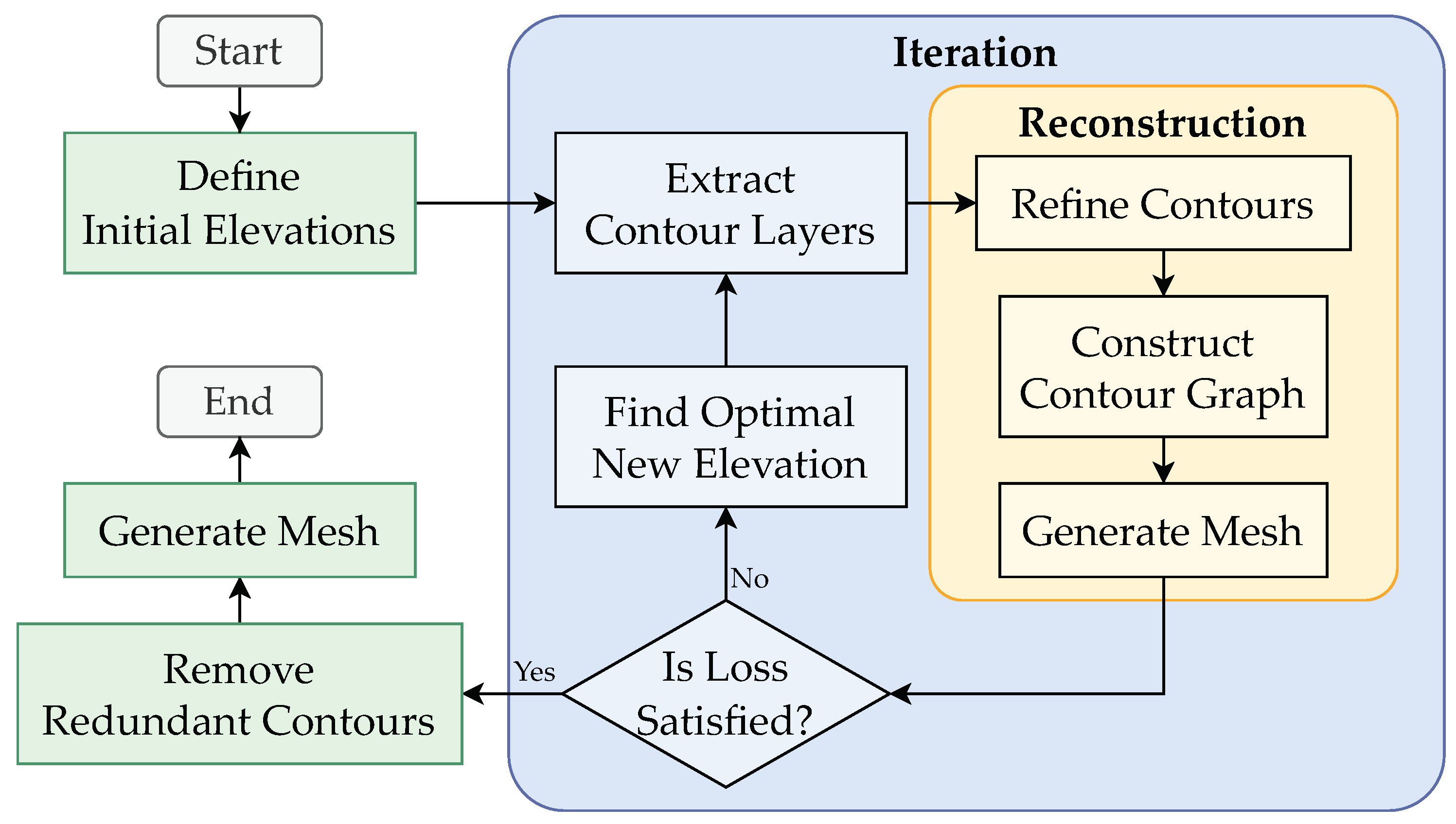
3.1. Overview

In this study, we introduce a novel iterative contour-based method to generate low-poly building meshes from mesh soups. An iterative pipeline is used to gradually extract vital contours for low-poly mesh reconstruction. In each iteration, the optimal new contours are determined by the difference between the current result and the input. The overall pipeline of our method is illustrated in Figure 1.

To produce a low-poly mesh based on contour, two primary targets are considered in our pipeline:

• Reduce the total number of contours.
  As mesh surfaces are generated from the contours, the compactness of the reconstructed meshes is bound to the total number of contours. Wu et al. [16] extract contours on evenly spaced elevations, while most of the contours are redundant as they have similar shapes to their neighbors. Zhang et al. [17] merge consecutive contours if they are identical to avoid duplicated contours. But, this method only handles contours with the same shapes and, thus, is not effective for the redundant contours on gradual slopes such as non-vertical walls and pitched roofs.
  To reduce redundant contours, our method only extracts vital contour layers (each contour layer contains all the contours on a specific elevation) near crucial elevations identified during the iteration. Moreover, as contours are extracted by layers, part of the contours in the contour layers may be redundant. A post-processing procedure is applied to remove this kind of redundant contour based on our contour interpolation algorithm.
• Generate compact surfaces between contours.
  • Raw contours extracted from the mesh soups usually contain a massive number of vertices with noise, while the sharp features (especially corners) are missing. Compact contours that contain only primary vertices with only essential details help obtain low-poly meshes. Traditional polygon simplification methods [29] (e.g., Ramer–Douglas–Peucker (RDP)) can effectively reduce noise and the number of vertices, but they lack the consideration of the sharp features and, thus, usually create undesirable bevels at corners. They also have trouble balancing between simplicity and detail preservation. Zhang et al. [17] provide a method to simplify axis-aligned structures while recovering right-angled corners by minimum circumscribed cuboids. But, this method produces zigzag artifacts on non-axis-aligned structures and fails to recover non-right-angled corners.
    To simplify contours while preserving essential details and sharp features, we utilized the planar primitives of the buildings. These primitives serve as references in our contour refinement, which produces compact contours with recovered sharp corners.
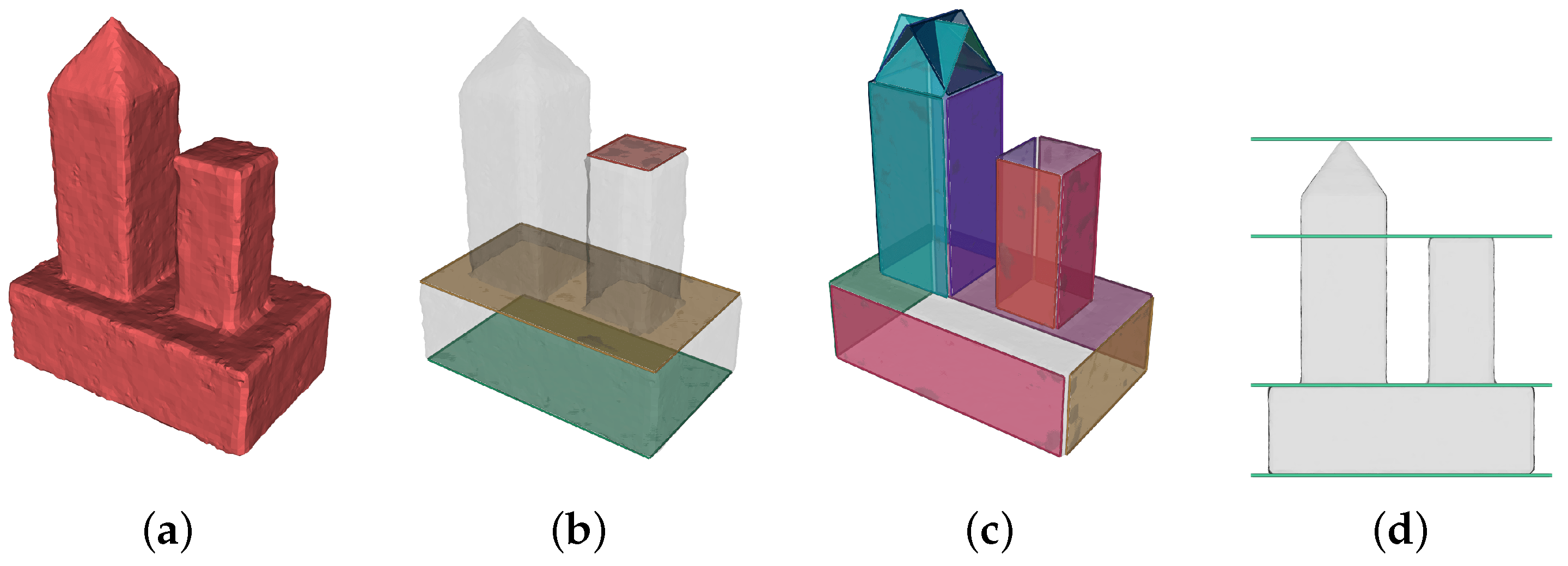
  • The connection relationships between contours should be recovered for the surface generation, and the contour graphs are utilized in the previous methods. Each node in the contour graph corresponds to a contour, and the edges indicate the connection between contours. For contours from the DSM, the contour graph falls back to a contour tree and can be constructed straightforwardly [30,31] as these contours follow the restriction that the higher contours must be contained by the lower contours. However, as mesh soups are not under this restriction, the construction of contour graphs is more difficult as the containment relationship between contours can be complicated due to noise or complex topology. For example, the lower contours can be reversely contained by higher contours or they can be only partially overlapped.
    To construct contour graphs for contours from mesh soups, we decompose the construction of contour graph into that of multiple bipartite graphs. Our method imposes no restriction and is capable of complex containment relationships between contours.
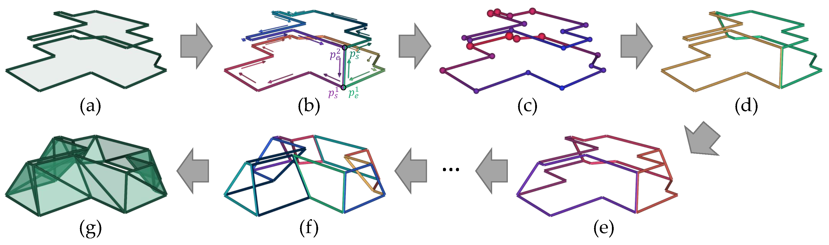
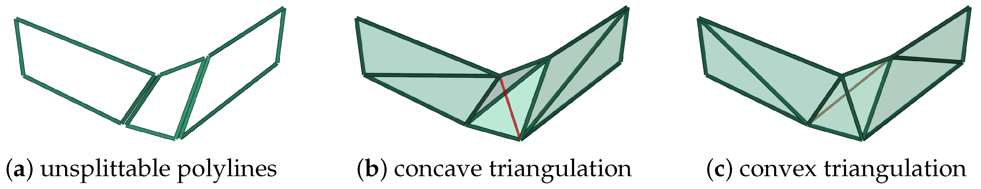
  • To generate surfaces between adjacent contour nodes, additional vertices may be inserted, which lead to extra faces and influence the compactness of the result. This challenge becomes more pronounced when the adjacent contours have significantly different shapes. Vertical extrusion and cuboid fitting [17] generate compact surfaces for identically shaped contours found on vertical walls and flat roofs. But, they can hardly generate non-vertical surfaces and, thus, produce staircase-like artifacts on slopes. Wu et al. [16] introduce a method to generate non-vertical surfaces for any pair of adjacent contour nodes by solving a bipartite-graph-matching problem, which successfully recovers the surface of slopes. But, this method resamples contours into dense vertices, which leads to enormous faces in the results. Moreover, an ambiguous topology caused by unsatisfactory matches may appear at sharp corners and complex sections of the contours, which makes it difficult to define the actual surface.
    We propose a method to generate compact surfaces between adjacent contour nodes by recursive polyline splitting. Our method has no restriction on the shape of the contours and produces surfaces with a restricted number of faces related to the compactness of the input contours.

Figure 2 shows a visual example of the primary stages in our pipeline. The details of the procedures and algorithms in our pipeline are outlined in the following sections.

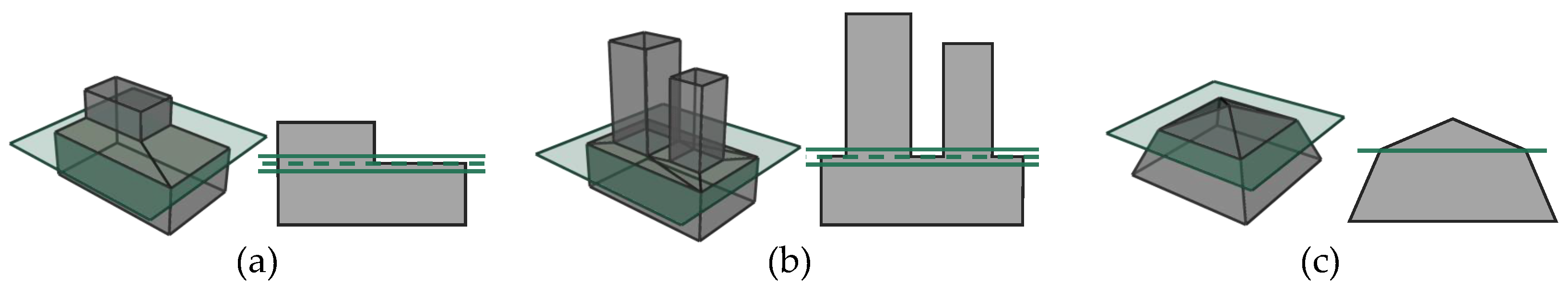
3.2. Iterative Crucial Elevation Identification

As generating contours on evenly spaced elevations produces a significant number of redundant contours, our iterative pipeline only extracts vital contours near crucial elevations. We assumed that the elevations with larger losses and topological variations are more-crucial, and these elevations were identified in an orderly manner during the iteration based on the current reconstructed result.

Initially, the iteration starts with several basic crucial elevations: the lowest and highest elevations of the building are used as they define the domain of elevation; the elevations of all horizontal planes in the building are also crucial as they indicate dramatic topological variations such as the ends of structure, changes of contour count, etc. The horizontal planes come from the planar primitives extracted from the building by common methods such as region-growing or RANSAC. Figure 3 shows an example of the extracted planes and initial crucial elevations.

Since there could be more-crucial elevations not included in the initial elevations, the remaining crucial elevations are identified during the iteration. In each iteration, the building is vertically divided into multiple segments by the current identified crucial elevations. Subsequently, the segment with the largest loss is chosen, and the optimal new elevation will be determined inside this segment. The loss of a segment is calculated by a loss defined as:

$$\mathrm{loss}(S,\widehat{S})=\frac{1}{n}\sum _{i=1}^n\underset{t}{min}\parallel p_i-q\left(t\right)\parallel$$

(1)

where S refers to the ground truth surface, $\{p_1,p_2,\cdots ,p_n\}\in S$ refers to an evenly sampled point cloud from S, $\widehat{S}=q\left(t\right)$ refers to the reconstructed surface, and $\parallel p_i-q\left(t\right)\parallel$ is the length of vector $p_i-q\left(t\right)$, which represents the Euclidean distance between these two points.

A new crucial elevation will be determined inside the chosen segment and added to the current result for the next iteration. As we assumed that the elevations with larger loss and topological variation are more crucial, several helper functions about loss and topological variation were constructed to find the optimal elevation. Specifically, the optimal elevation was chosen among a set of increasing, evenly spaced elevations $\{e_1,e_2,\cdots ,e_n\}$ with interval $d_{\mathrm{sample}}$(= 0.01–0.05 m) inside the segment. To measure the importance of each elevation, a priority function $P\left(e_k\right)(1\le k\le n)$ is defined. The function $P\left(e_k\right)$ is based on two other functions $D\left(e_k\right)$ and $V\left(e_k\right)$, where $D\left(e_k\right)$ indicates the loss and $V\left(e_k\right)$ indicates the topological variation at elevation $e_k$.

The loss function $D\left(e_k\right)$ is defined by the distance of the contours. At each elevation $e_k(1\le k\le n)$, the corresponding set of contours from the ground truth mesh (denoted as $C_k$) and that from the reconstructed mesh (denoted as ${\widehat{C}}_k$) are extracted. Subsequently, their distance is measured by a Chamfer-distance-like function defined as:

$$\mathrm{distance}(C,\widehat{C})=\frac{1}{2\left|C\right|}{\int }_s\underset{t}{min}\parallel p\left(s\right)-q\left(t\right)\parallel ds+\frac{1}{2|\widehat{C}|}{\int }_t\underset{s}{min}\parallel q\left(t\right)-p\left(s\right)\parallel dt$$

where $C=p\left(s\right)$, $\widehat{C}=q\left(t\right)$, and $\left|C\right|$, $|\widehat{C}|$ denote the total perimeter of each contour set. Considering the performance issue, the actual distances are calculated using the discrete form of this function by evenly sampling n ($n=1000$) points from each set of the contours along the edges, which is:

$$\mathrm{distance}(C,\widehat{C})=\frac{1}{2n}(\sum _{i=1}^n\underset{j=1}{\overset{n}{min}}\parallel p_i-q_j\parallel +\sum _{j=1}^n\underset{i=1}{\overset{n}{min}}\parallel q_j-p_i\parallel )$$

(2)

where $\{p_1,p_2,\cdots ,p_n\}\in C,\{q_1,q_2,\cdots ,q_n\}\in \widehat{C}$ refer to the sampled points of the two contour sets. The distances of contours at each elevation form a function $D\left(e_k\right)=\mathrm{distance}(C_k,{\widehat{C}}_k)$, which signifies the distribution of the loss at different elevations.

To identify the changing of a building topology, a topological variation function $V\left(e_k\right)$ is defined based on the variation of the loss with the following steps. For each point $(e_k,D\left(e_k\right))$ in $D\left(e_k\right)$, its preceding m points (m = 5–20, depends on the sample interval $d_{\mathrm{sample}}$) are gathered and form a set of points $\{(e_i,D\left(e_i\right))\mid k-m\le i\le k\}$. Principal component analysis (PCA) is performed on the point set to calculate the main direction $v_{-}\left(e_k\right)$, which indicates the variation trend of the building topology below elevation $e_k$. Similarly, the variation trend $v_{+}\left(e_k\right)$ above elevation $e_k$ is also calculated. If the above and below variation trends point to significantly different direction, this implies a sharp corner in the loss function, and there is likely to be a dramatic topological variation at elevation $e_k$. Therefore, the topological variation function is defined as $V\left(e_k\right)=1-v_{-}\left(e_k\right)·v_{+}\left(e_k\right)$, which signifies the variation of the building topology at elevation $e_k$.

As we assume that the elevations with larger loss and topological variation are more crucial, a priority function $P\left(e_k\right)=D\left(e_k\right)V\left(e_k\right)$ is defined to measure the importance of elevations. The maximum point of $P\left(e_k\right)$ is determined, and the corresponding elevation is used as the new elevation.

Crucial elevations are identified during the iteration with the above procedures. The iteration stops when the loss of the reconstructed mesh is satisfied (<80–150 mm, measured by Equation (1)) or there are no more valid new elevations. An example of the iteration is presented in Figure 4.

3.3. Contour Layer Extraction

For each crucial elevation e, directly extracting contours at e may result in poor contours with too much noise and fail to capture nearby information if there is a dramatic topological variation. We, thus, used different strategies to extract contours for different circumstances.

To check if dramatic topological variation exists at e, a bias $\beta$ (=0.2–0.6 m, depends on the density and noise of input data) is defined, and two contour layers at elevations $e-\beta$ and $e+\beta$ are extracted. Subsequently, a bipartite graph is constructed for the two contour layers (the construction of the bipartite graph is explained in Section 3.4.2). If nodes in the graph are doubly linked in pairs, which indicates that every contour has exactly one identical contour in the other layer, we assumed that there is no dramatic topological variation. Otherwise, a dramatic topological variation is present at this elevation.

For elevation e without dramatic topological variation, extracting contours at elevation e is deemed safe. The contour layer at elevation e is directly extracted and, then, added to the current result. Otherwise, to completely capture the nearby information while avoiding poor contours, the two contour layers at $e-\beta$ and $e+\beta$ are both added to the current result, and no further contour layer is allowed to be extracted between them thereafter. Examples of these two circumstances are given in Figure 5.

3.4. Low-Poly Mesh Reconstruction

A low-poly mesh can be reconstructed from the extracted vital contours with three steps: contour refinement, contour graph construction, and low-poly surface generation.

3.4.1. Contour Refinement

The raw contours contain a massive number of vertices with noise, while corners are missing and replaced by undesirable bevels. Moreover, our method extracts contours near crucial elevations, which are frequently located at structures with dramatic topological variations. The contours, thus, have more noise and larger deformation.

To obtain compact contours with only essential details for compact surface generation, we utilized the planar primitives of buildings and refined the contours with three steps: vertex attaching, corner recovery, and simplification.

Initially, a vertex-attaching procedure was performed to reduce the noise, where the vertices will be projected to the optimal reference line generated from the planar primitives. Specifically, for each contour, its corresponding co-planar horizontal plane is created and, then, intersects with the extracted non-horizontal planes (as shown in Figure 3c) of the buildings. The intersection lines are used as reference lines for vertex attaching. For each vertex on the contour, all near reference lines that are closer than a tolerance $t_{\mathrm{attach}}$ (=0.2–0.5 m) are collected as candidates. To find the optimal candidate line, the weight of each line is defined by the included angle and distance, which is:

$${\mathrm{Weight}}_{\mathrm{attach}}(l,p,n_p)=\frac{|n_l·n_p|}{\parallel p-p_{\perp }\parallel }$$

where l refers to the candidate reference line, $n_l$ refers to the normal of the line, p refers to the vertex, $n_p$ refers to the normal of vertex, which is defined as the average normal of its connected edges, and finally, $p_{\perp }$ refers to the nearest point to p on line l. The line with the largest weight is chosen, and vertex p will be attached to it by shifting its coordinate to the corresponding $p_{\perp }$.

After the vertex attaching, missing corners are recovered in our corner-recovery procedure by the intersections of the lines. For each pair of adjacent vertices $(p_1,p_2)$ in contours that are attached to two different lines, the intersection point $p_{\mathrm{corner}}$ of the two lines represents a corner point. If the Euclidean distance between $p_{\mathrm{corner}}$ and $\frac{p_1+p_2}{2}$ is smaller than a tolerance $t_{\mathrm{corner}}$ (=2$t_{\mathrm{attach}}$), $p_{\mathrm{corner}}$ is added to the contour as a new vertex between $p_1$ and $p_2$, and hence, a missing corner is recovered. After recovering these corners, all co-linear adjacent edges are merged to remove redundant vertices.

Additionally, the vertex attaching may not be helpful when there are no reference lines, which could happen on non-planar surfaces. A traditional polygon-simplification algorithm is performed after the above steps to handle this situation. As the mesh soups are usually generated from the scanning data, the noise of the meshes mainly comes from the vertices. We, thus, chose the RDP algorithm with tolerance $t_{\mathrm{rdp}}$ (=0.8$t_{\mathrm{attach}}$) for simplification, as it uses metrics based on the vertex distance.

After performing the procedures described above, the contour obtains fewer vertices and less noise, while the sharp corners are recovered. Figure 6 shows an example of the contour refinement at all stages.

3.4.2. Contour Graph Construction And Post-Processing

To restore the connection relationship between contours for surface generation, a contour graph will be constructed using our method. Our contour graph construction method imposes no restriction and is capable of complex containment relationships between contours. Moreover, a post-processing procedure will be applied after the completion of iterations to remove potential redundant contours based on our contour interpolation algorithm.

Our method decomposes the construction of the whole contour graph into that of multiple bipartite graphs. For each pair of adjacent contour layers, a directed bipartite graph is constructed, and then, these graphs are merged into a complete contour graph. In the directed bipartite graph, nodes and contours are in one-to-one correspondence. A directed edge between nodes signifies that the contour of the start node is contained by the contour of the end node (or the start node is contained by the end node for short). Due to the topological restriction on buildings, the directed bipartite graph must satisfy the following restrictions:

• Each node has at most one outgoing edge, as a contour can only be contained by at most one contour in the other layer.
• A node should not have both an incoming edge and outgoing edge at the same time, except when these two edges are reverse edges of each other. For the latter circumstance, the two contours contain each other, which is allowed as this indicates that they have an identical shape. Otherwise, a sequence of containment exists, further deriving that one contour is contained by another contour in the same layer, which is impossible.

A verification is defined for the restriction to check if two contours $(C_1,C_2)$ are identical. The distance between the two contours is calculated by Equation (2), and they are considered identical if the distance is smaller than a tolerance $t_{\mathrm{identical}}=0.05min(A_{C_1},A_{C_2})$, where $A_{C_1}$ and $A_{C_2}$ are the area of the two contours.

Based on these restrictions, we propose a greedy edge-selection algorithm to construct the directed bipartite graph under the restrictions for each pair of adjacent contour layers.

Initially, candidate edges are generated by creating every possible edge for the directed bipartite graph. These candidate edges connect every pair of nodes in different contour layers.

Subsequently, suitable edges are selected from these candidates with the following steps. The candidate edges are sorted by weight in descending order. The weight of an edge $({\mathrm{node}}_s,{\mathrm{node}}_e)$ is defined by the degree of containment between them, which is:

$${\mathrm{Weight}}_{\mathrm{edge}}({\mathrm{node}}_s,{\mathrm{node}}_e)=1-2\frac{A_{(C_e-C_s)}}{A_{C_e}}\in [-1,1]$$

where $C_s,C_e$ refers to the contours of ${\mathrm{node}}_s,{\mathrm{node}}_e$, A refers to the area of a geometry, and subtraction between geometry refers to the Boolean difference of them. All candidate edges with negative weights are removed due to the weak containment relationships.

Starting with a graph with only nodes and no edges, edges will be added step by step by traversing and selecting from the sorted candidate edges. For each candidate edge, it will be added to the graph if the restriction is still satisfied after adding this edge; otherwise, the edge will be discarded. A directed bipartite graph is constructed after traversing these candidate edges.

For each constructed directed bipartite graph, the nodes of the graph will be grouped for later surface generation. The constructed directed bipartite graphs will be converted into undirected bipartite graphs, which can, then, be separated into one or multiple connected components. Each connected component represents a group of nodes. With the restriction above, only three types of node groups are present in the graph:

• 1-0 group: consists of only one node with no edge.
• 1-1 group: consists of two nodes with one or two edges. One of the nodes contains the other node, or the two contours of nodes are identical.
• 1-n group ($n>1$): consists of 1 node in one layer, n nodes in the other layer, and n edges. The independent 1 node contains all the n nodes in the other layer.

Note that the n-m ($n>1,m>1$) group will not appear in the graph as it breaks the restrictions.

After constructing all the bipartite graphs, the complete contour graph is created by merging all these bipartite graphs. Two examples of the contour graph construction are shown in Figure 7a–c.

Since there may still be potential redundant contours in the graph after the completion of the iterations, a post-processing procedure is applied to the graph to remove these contours based on our contour interpolation algorithm.

Initially, nodes in the contour graph at the same branches are clustered, where each cluster contains a continuous sequence of nodes. To be specific, all edges in the 1-n node groups are temporarily removed, and each connected component in the remaining graph forms a node cluster.

Subsequently, redundant contours are removed by verifying if they can be restored from their neighbors within each cluster. For the k-th node with elevation $e_k$ and contour $C_k$ (denoted as $(e_k,C_k)$) in a node cluster with n nodes ($1<k<n$), an interpolated contour ${\overline{C}}_k$ is generated from its adjacent nodes $(e_{k-1},C_{k-1})$ and $(e_{k+1},C_{k+1})$ using our contour-interpolation algorithm (see the details in Section 3.4.3). If ${\overline{C}}_k$ and $C_k$ are identical (judged by the verification defined before), $C_k$ is considered redundant and will be marked as a removal candidate. The removal candidate with the smallest contour distance will be removed, while its connected edges will be fused, and the node groups will be updated. This removal procedure repeats on the updated cluster until there are no more redundant contours. Figure 7d shows two examples of the post-processing.

3.4.3. Low-Poly Surface Generation

As the contours in the graph are compact after the previous refinement procedure, we aimed to generate compact surfaces from these contours while preserving their compactness. The generation of mesh surfaces consists of two parts: interior faces and boundary faces. The interior faces form the surfaces between contours such as wall and pitch roofs (Figure 8b), while the boundary faces form the horizontal surfaces such as flat roofs, which usually occur at terminal nodes (Figure 8c).

Interior faces are generated at each node group with different strategies depending on the type of group:

• 1-0 group: no interior face.
• 1-1 group: interior faces are generated using our contour-interpolation algorithm.
• 1-n group ($n>1$): contours of the n nodes are vertically extruded (without caps) to fill the in-between space.

The interior faces of 1-1 group are generated using our contour-interpolation algorithm. Initially, given a 1-1 group with two adjacent contour nodes $(C_1,C_2)$, the nearest pair of vertices between the two contours is determined and, then, connected by a new edge. This edge connects the two contours and creates a closed polyline denoted as $(p_s^1,p_e^1,p_s^2,p_e^2)$ (as shown in Figure 9b), where $p_s^1,p_e^1,p_s^2,p_e^2$ refer to its start and end points on both contours. Subsequently, the polyline will be split into two new polylines by an optimal split position determined by the distance. The same splitting procedure repeats on new polylines until the polylines are unsplittable, which means no valid split can be found anymore. An unsplittable polyline has exact n and m vertices on the two contours, where $n+m=3(n,m\ge 1)$ (triangle) or $n=m=2$ (quadrilateral).

To balance the two new polylines for better results, the optimal split position is determined from the vertices by distance. For a polyline $(p_s^1,p_e^1,p_s^2,p_e^2)$, the distance of the vertex is defined as the sum of the minimum distances from the vertex to two edges $(p_s^1,p_e^1)$ and $(p_s^2,p_e^2)$. The vertices are sorted by this distance in descending order, and the first valid split will be applied.

To split the polyline with a vertex p on one contour of the polyline, its closest point $p_{\mathrm{new}}$ on the other contour is determined, while the corresponding edge $(p_{new}^{-},p_{new}^{+})$ that $p_{\mathrm{new}}$ falls within is also determined (an example is shown in Figure 10b). To avoid adding redundant vertices, a merge tolerance $t_{\mathrm{merge}}$ (=2 m) is defined. If the distance from $p_{\mathrm{new}}$ to $p_{new}^{-}$ or $p_{new}^{+}$ is closer than $t_{\mathrm{merge}}$, $p_{\mathrm{new}}$ is shifted to the nearest vertex $p_{new}^{-}$ or $p_{new}^{+}$. A comparison of the results with and without merging is shown in Figure 10.

Subsequently, a split edge $(p,p_{\mathrm{new}})$ is created, and if the edge splits the polyline into two new valid closed polylines (number of vertices ≥ 3), the split is considered valid.

After the optimal split, two new polylines are created in place of the original polyline, and these new polylines will also be split if they are still splittable. Eventually, the initial polyline will be split into multiple unsplittable polylines, which will be used for surface generation and contour interpolation. To generate an interpolated contour between the two contours, all split edges will be interpolated and, then, the interpolated points are connected to form the target contour.

Based on these unsplittable polylines, the surfaces are generated with a triangulation procedure. Two types of unsplittable polylines are present in the results: triangle polylines and quadrilateral polylines. For a triangle polyline, a triangle face can be directly created by its three vertices. For a quadrilateral polyline, there are two choices of triangulation since the polyline may not be planar, and the convex one is chosen as shown in Figure 11.

With the polyline splitting and triangulation, interior faces between two contours are generated with only a small number of additional vertices, which keeps the compactness of the contours. An example of polyline splitting and triangulation is shown in Figure 9.

As the interior faces form the main surfaces of the building, but leave holes in the mesh, the boundary faces are generated to enclose these holes. The contours of all terminal nodes (with degrees of 1) form faces to fill part of the holes (Figure 8c, red faces), while the remaining holes appear at 1-n groups. Faces are generated to fill these holes by the symmetric difference of two contour layers (Figure 8c, blue faces), which is defined as $C_0\Delta {\bigcup }_{i=1}^n{C}_i$ with the same elevation as $C_0$, where $C_0$ refers to contour of the independent 1 node, $C_i(1\le i\le n)$ refers to contour of the i-th node in the n nodes, and $\Delta$ refers to the Boolean symmetric difference of two geometries.

The interior faces and boundary faces are generated using the above methods, and these faces form a watertight mesh. Examples of interior and boundary face generation are shown in Figure 8.

4. Results And Evaluation

4.1. Dataset

We used the Helsinki [32] dataset to evaluate the effectiveness of our method. The Helsinki dataset consists of two parts: semantic city information models (denoted as semantic models) and visually high-quality reality mesh models (denoted as reality models). The semantic models provide monomerized and low-poly building meshes, while the reality models contain mesh soups of various items created from aerial photographs.

The low-poly building meshes in the semantic models were converted into noisy mesh soups for the experiments. Specifically, these low-poly meshes were sampled into point clouds (1 points/m²) with disturbing on the normal to simulate noise, where the disturbance follows a Gaussian distribution $\mathcal{N}(0,{\sigma }^2)$. Subsequently, Poisson reconstruction was performed on the noisy point clouds to generate noisy mesh soups, and these mesh soups were used as the inputs in the experiments. Meanwhile, the original low-poly meshes were used as the ground truth in the experiments. Examples of the generated mesh soups are shown in Figure 12.

Additionally, to demonstrate the effectiveness of our method on realistic data, four buildings in the reality models were manually monomerized and used as the input in the experiments. As there were no ground truth meshes for the reality models, these mesh soups were directly regarded as the ground truth in the result evaluation.

4.2. Comparison with Previous Methods

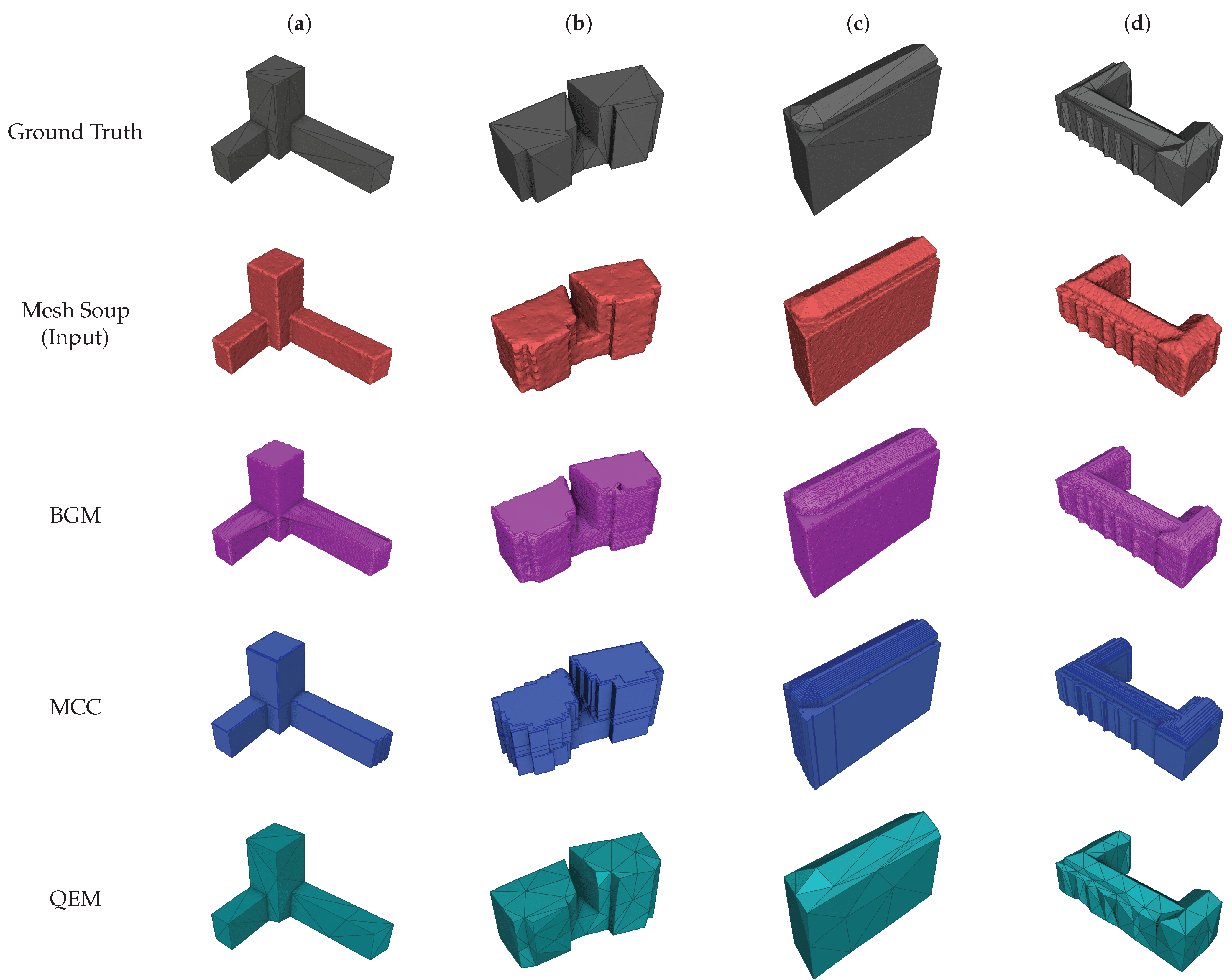
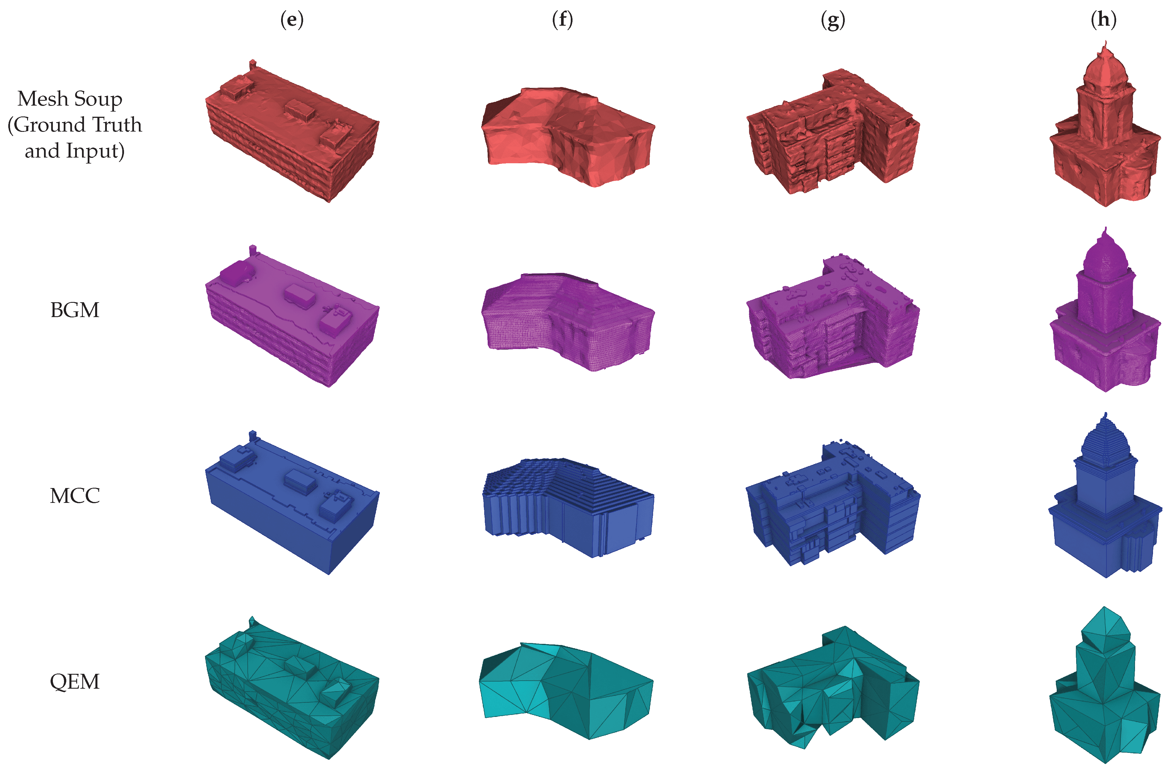
4.2.1. Comparison of General Effectiveness

To evaluate the general effectiveness of our method, we compared our method with three other methods. Two of them are also based on contours, and one, from Wu et al. [16], uses bipartite graph matching for contour interpolation (denoted as BGM), while the other, from Zhang et al. [17], uses the minimum circumscribed cuboids method for surface fitting (denoted as MCC). The third method is QEM [27], which is a general mesh simplification method based on edge-collapsing. The target of QEM is set as reaching the same number of triangles as our result for comparison.

The experiments used one hundred buildings from the Helsinki semantic models, which were converted into mesh soups with various intensities of disturbance ($\sigma =$ 0.05, 0.1, 0.15, 0.2), and four buildings from the reality models. These building mesh soups were reconstructed using each method, and the summary of the evaluations is shown in

Table 1. Average losses, number of triangles, and number of contours at different noise levels for each method.

	Methods	$\mathit{\sigma }=0.5$	$\mathit{\sigma }=0.1$	$\mathit{\sigma }=0.15$	$\mathit{\sigma }=0.2$
Average Loss (mm)	BGM	94.1	98.6	104.8	111.5
	MCC	117.6	116.8	117.0	117.2
	QEM	121.1	176.4	180.5	217.2
	Ours	91.0	94.0	102.6	114.6
Average Number of Triangles	BGM	40,690.2	44,838.2	48,453.5	54,032.4
	MCC	1105.6	1266.7	1413.1	1614.2
	QEM	163.8	208.0	232.9	305.9
	Ours	163.8	208.0	232.9	305.9
Average Number of Contours	BGM	68.2	75.2	81.2	90.5
	MCC	30.8	36.2	40.7	47.2
	Ours	6.4	7.6	8.0	9.9

, where the loss is calculated by Equation (1). Some examples of the results are shown in Figure 13 (semantic models) and Figure 14 (reality models), where the statistics of these results are listed in

Table 2. Statistics of the reconstruction results in Figure 13 and Figure 14.

Data	Building	Methods	Loss (mm)	Number of Contours	Number of Triangles
semantic models	(a) $\sigma =0.05$	BGM	64.9	95	56,760
		MCC	124.5	10	476
		QEM	89.1	—	40
		Ours	54.4	4	40
	(b) $\sigma =0.1$	BGM	98.9	65	38,840
		MCC	125.3	22	1368
		QEM	94.7	—	155
		Ours	119.8	6	155
	(c) $\sigma =0.15$	BGM	75.9	279	165,582
		MCC	207.8	116	2425
		QEM	522.0	—	50
		Ours	57.5	5	50
	(d) $\sigma =0.2$	BGM	111.0	75	44,848
		MCC	124.4	46	2268
		QEM	205.2	—	198
		Ours	146.8	5	198
reality models	(e)	BGM	74.6	98	58,679
		MCC	106.7	74	1084
		QEM	75.1	—	317
		Ours	224.2	16	317
	(f)	BGM	37.6	55	32,690
		MCC	172.1	48	2545
		QEM	743.1	—	66
		Ours	163.7	5	66
	(g)	BGM	78.5	255	151,765
		MCC	124.2	174	3104
		QEM	214.7	—	157
		Ours	168.8	4	157
	(h)	BGM	50.1	121	72,467
		MCC	135.8	106	1692
		QEM	243.3	—	90
		Ours	260.5	6	90

.

The analyses of results for each method are listed below:

• BGM generates contours on evenly spaced elevations, and each contour is resampled into a fixed number of vertices for surface generation. The reconstructed meshes obtain small losses, but contain a significant number of faces. Moreover, it generates incorrect connections at some dramatically changing elevations (e.g., (a) and (g)), and an ambiguous topology may appear at sharp corners or complicated sections of the contours (see the details in Section 4.2.3).
• MCC produces compact surfaces on axis-aligned structures with the sharp corners recovered (e.g., (a)) under the assumption that the input buildings are comprised of axis-aligned cuboids. However, since MCC lacks an additional strategy to handle non-axis-aligned structures, they tend to be fit by multiple axis-aligned edges, which generate zigzag artifacts and cost more vertices (e.g., (b) and (f)). Meanwhile, the pitched roofs are reconstructed into dense cuboids, leading to staircase structures in the results (e.g., (c), (d), (f), and (h)). Consequently, higher losses and denser faces are present in the results compared to the axis-aligned structures. Additionally, the results of BGM and MCC also suffer from poor contours found on dramatically changing elevations due to the evenly spaced contour-generation strategy (e.g., roofs of (e) and (g)).
• QEM iteratively collapses edges based on the quadric error metric to simplify the mesh soups and is able to reach an arbitrary target number of triangles. Nevertheless, the QEM method is designed for general purposes and does not consider the structure of buildings in its metric, which brings the challenge of balancing between simplicity and detail preservation. The surfaces that are supposed to be planar usually become bumpy, while the sharp corners are over-smoothed (e.g., (b) and (d)). Moreover, the QEM has difficulty preserving the general structure of buildings under an excessive strength of simplification, which significantly increases the loss (e.g., (c) and (f)). Therefore, the QEM method obtains higher losses on average compared to other methods, as shown in the experimental results.
• Our method only generates vital contours and removes redundant contours if they are restorable, thus using much fewer contours compared to other contour-based methods. Our method also prevents directly extracting contours at dramatically changing elevations to avoid poor contours compared to the evenly spaced contour-generation strategy. Furthermore, accurate corners are recovered in our corner-recovery procedure with the guide of planar primitives, and thus, fewer unnecessary bevels at corners are present in our results. Based on the refined contours, compact surfaces can be generated using our contour-interpolation algorithm. Our method, thus, produces low-poly results with small losses compared to other methods.

In conclusion, our method shows the ability to generate compact meshes compared to the previous contour-based method and the QEM method.

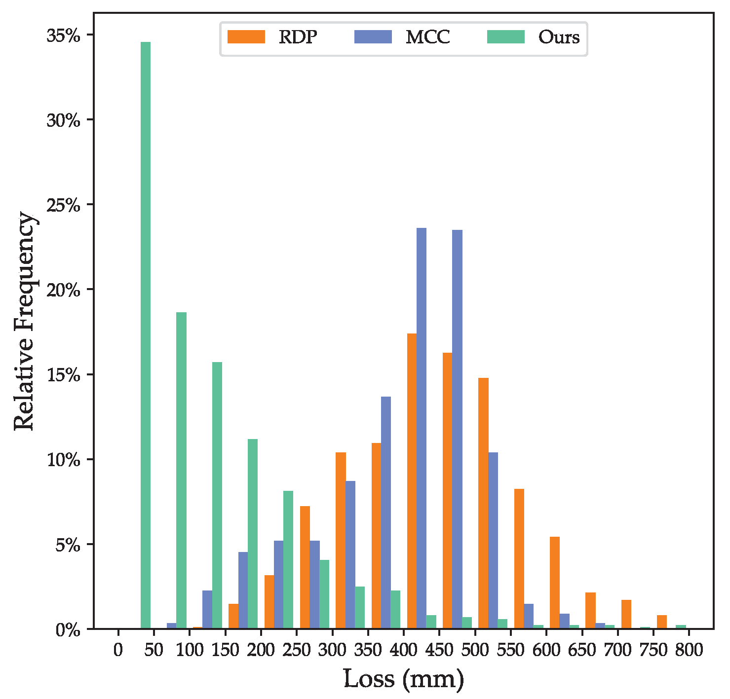
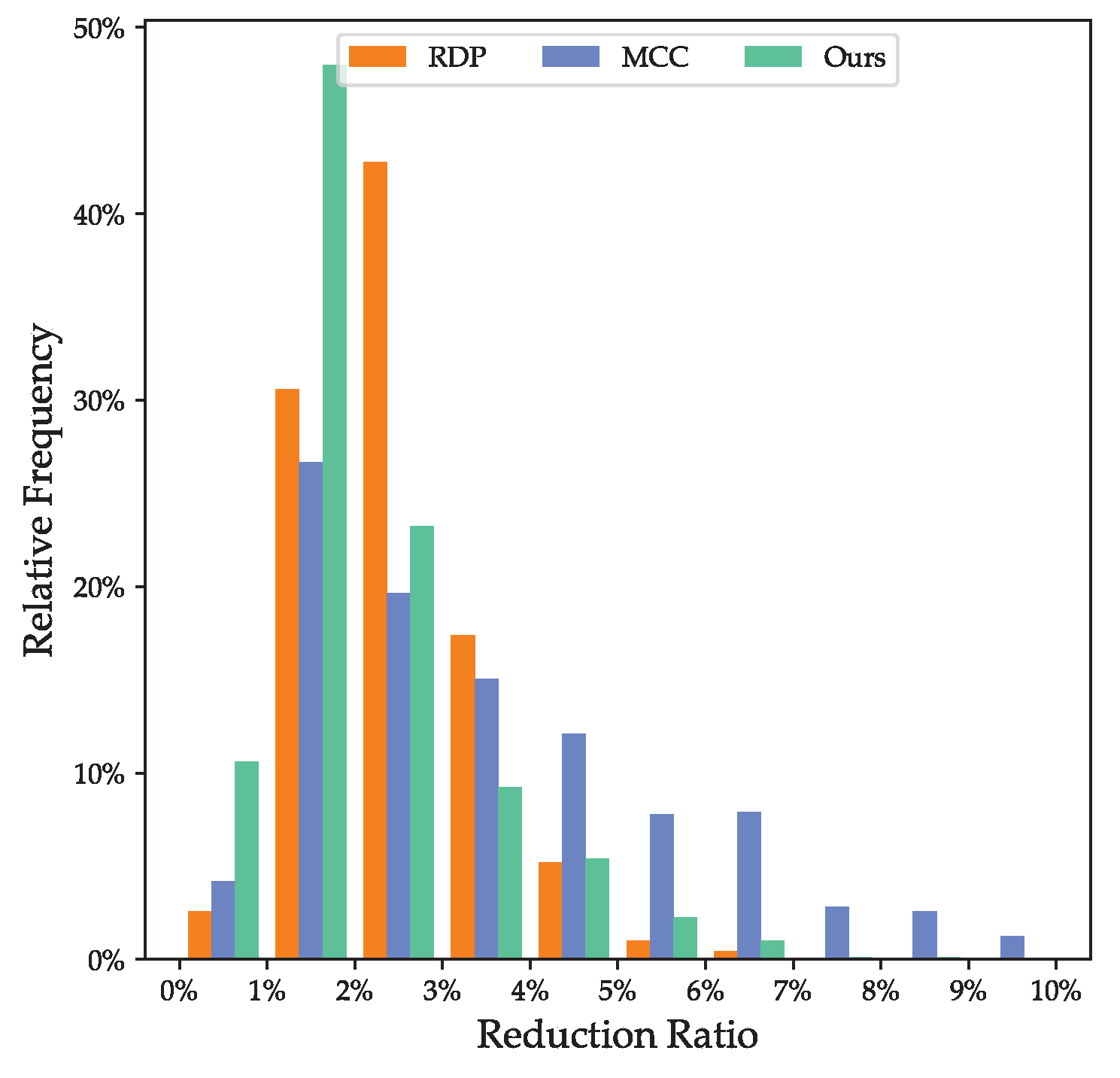
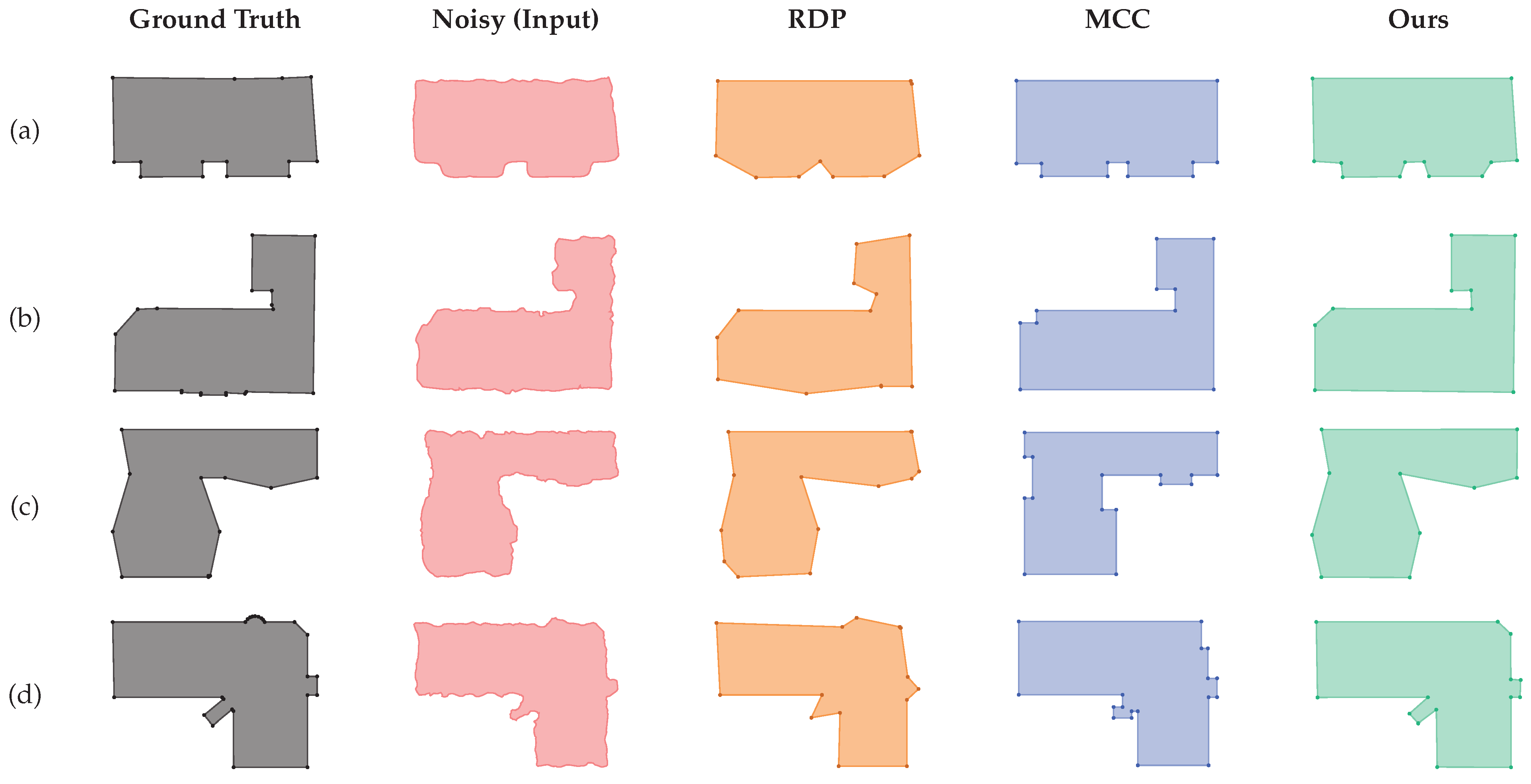
4.2.2. Comparison of Contour Refinement

We propose a contour refinement method to obtain compact contours from the raw noisy contours while recovering sharp corners. To evaluate the effectiveness of our method, we compared our method with the RDP and MCC methods.

The experimental data were gathered from the semantic models. Pairs of contours near crucial elevations were extracted. For each pair of contours, the original low-poly mesh produces one simple, compact contour, serving as the ground truth, while the corresponding mesh soup ($\sigma$ = 0.2) produces the other noisy, complex contour, serving as the input. After the refinement of these noisy contours, losses (measured by Equation (2)) and geometric complexities of the results are evaluated for each method.

Figure 15 illustrates the distribution of the losses, and Figure 16 shows the distribution of the reduction ratio (defined as the ratio of the vertex count between the result and the input) for each method. The summary of the losses and reduction ratios is listed in

Table 3. Summary of contour refinement results.

Methods	Average Loss (mm)	Average Reduction Ratio	Average Number of Vertices
RDP	446.5	2.48%	12.2
MCC	398.8	3.47%	19.0
Ours	124.3	2.09%	10.4

. Some examples of the results are shown in Figure 17, while their corresponding statistics are listed in

Table 4. Statistics of the contour refinement results in Figure 17.

Contour	Number of Vertices	Methods	Loss (mm)	Number of Vertices
(a)	14	RDP	330.0	10
		MCC	228.6	12
		Ours	64.0	12
(b)	19	RDP	528.5	12
		MCC	397.1	10
		Ours	107.8	9
(c)	13	RDP	433.6	13
		MCC	556.9	16
		Ours	55.2	10
(d)	25	RDP	504.2	14
		MCC	366.3	18
		Ours	65.3	14

.

The analyses of results for each method are listed below:

• RDP can efficiently remove vertices, but preserves the undesirable bevels at corners (e.g., (c)). Additionally, the tolerance of RDP is difficult to determine as a larger tolerance improves effectiveness on denoising, but small details are more likely to be erased (e.g., (a) and (d)).
• MCC assumes that buildings are formed with cuboids and generates compact results on axis-aligned edges with the corners recovered (e.g., (a), (b), and (d)). On the other hand, the non-axis-aligned edges are reconstructed into zigzag structures (e.g., (c) and part of (d)), leading to increased loss and excessive vertices.
• Our method takes advantage of the planar primitives of buildings in the vertex attaching for denoising, which produces more-accurate results compared to RDP. Moreover, our strategy of corner recovery has superior effectiveness without the axis-aligned limitation compared to MCC. Therefore, our method exhibits the ability to simultaneously simplify the contours and recover accurate corners, as shown in the results.

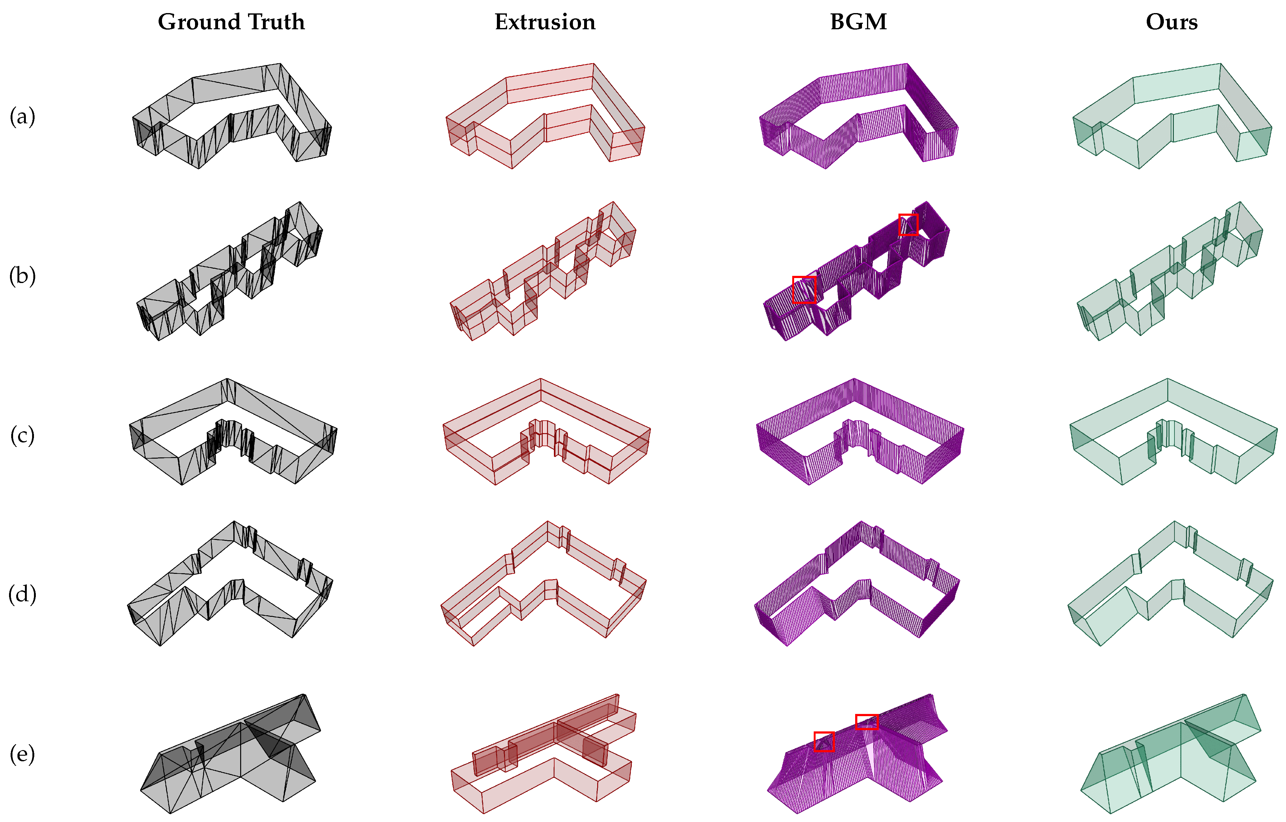
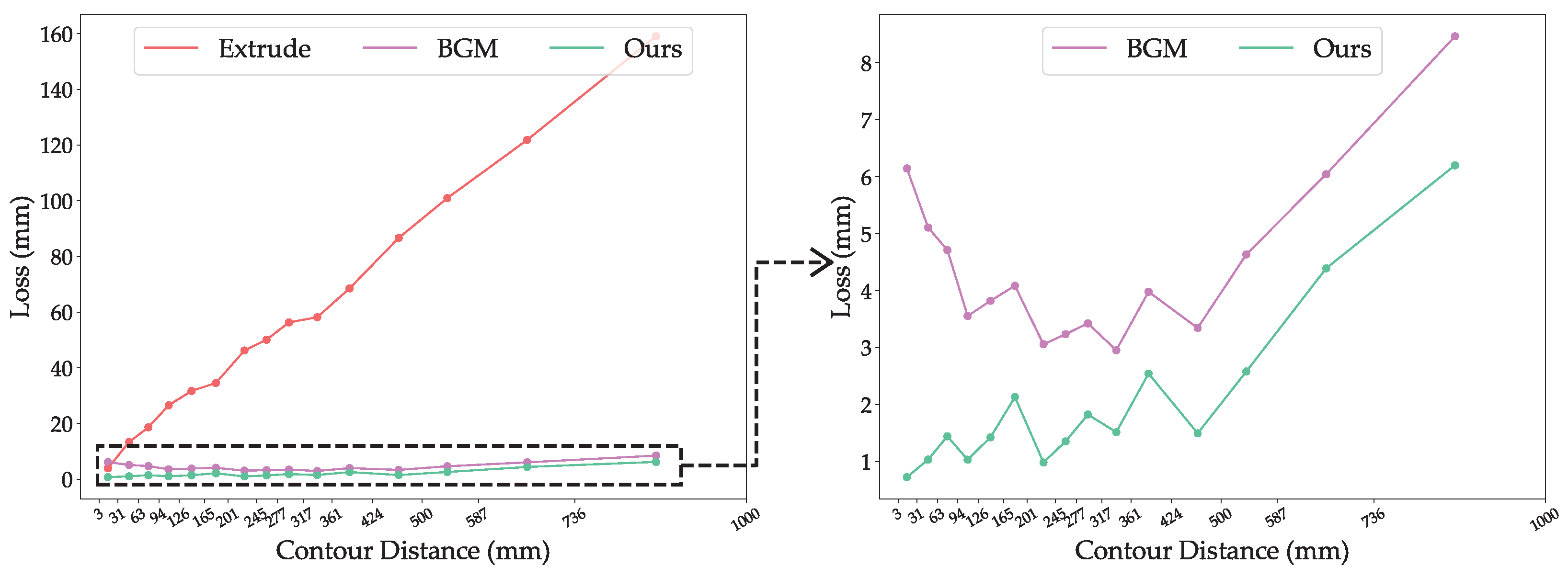
4.2.3. Comparison of Surface Generation

We propose a contour-interpolation algorithm to generate surfaces between adjacent contour nodes while preserving compactness. To demonstrate its effectiveness, we compared our method with the direct extrusion method (denoted as extrusion) and the bipartite graph matching methods (denoted as BGM). Given two adjacent contour nodes, the direct extrusion method vertically extrudes both contours towards each other by half of their interval to generate the surfaces.

Similar to the contour-refinement experiments, the experiment data were gathered from the semantic models. Pairs of high and low contours were extracted as the input. For each pair of contours, meshes were clipped by the two contours, and the clipped in-between surfaces were used as the ground truth. For each pair of contours, surfaces were generated using each method, and then, the losses (measured by Equation (1)) and numbers of faces were evaluated.

The experiment data were divided into two parts for better comparison: the “same-pair” part, where the paired contours are identical (with a distance of ≤5 mm measured by Equation (2)), and the remaining data fell into the “different-pair” part, where the paired contours are significantly different.

Table 5. Summary of “same-pair” surface-generation results.

Methods	Average Loss (mm)	Average Number of Triangles
Extrusion	0.00114	115.0
BGM	1.57457	600.0
Ours	0.00012	57.5

shows the results for the “same-pair” part, and examples are shown in Figure 18a,b, while the statistics of the two results are shown in

Table 6. Statistics of the surface-generation results in Figure 18.

Contour Pair	Distance (mm)	Number of Vertices	Methods	Loss (mm)	Number of Triangles
(a)	0.5	22	Extrusion	0.00064	44
			BGM	1.1	600
			Ours	0.00006	22
(b)	1.2	68	Extrusion	0.00012	136
			BGM	2.1	600
			Ours	0.00011	68
(c)	228.1	42	Extrusion	35.3	84
			BGM	1.6	600
			Ours	0.2	42
(d)	617.8	42	Extrusion	495.9	84
			BGM	3.5	600
			Ours	0.05	42
(e)	2796.6	20	Extrusion	699.0	40
			BGM	24.1	600
			Ours	3.5	22

. As there is no significant difference between the pair of contours, the extrusion method is sufficient to accurately recover the surface. For BGM, as the topology restriction is not considered in the bipartite graph matching, an ambiguous topology may appear at sharp corners and complicated sections of contours caused by an unsatisfactory match (marked by red rectangles in Figure 18). This led to higher loss compared to extrusion. In our method, the polylines were split based on the nearest points and vertex merging. Our method, thus, produces the same accurate, compact results as the extrusion.

For the “different-pair” part, as there are significantly more small-distance contour pairs than large-distance pairs, results were grouped by distance and, then, summarized for better clarity. The contour pairs were incrementally sorted by distance and evenly divided into fifteen groups. Subsequently, the average contour distance and loss of each group were calculated and, then, formed a line chart, as shown in Figure 19. Some examples of the results are shown in Figure 18c–e, and the corresponding statistics are also listed in

Table 7. Summary of “different-pair” part surface-generation results.

Methods	Average Loss (mm)	Average Number of Triangles
Extrusion	86.0	155.5
BGM	6.3	600.0
Ours	3.7	79.1

.

The analyses of results in the “different-pair” part for each method are listed below:

• The extrusion method exhibits significantly worse effectiveness at large-distance pairs of contours, as extrusion is not capable of generating non-vertical surfaces between contours.
• BGM can generate gradual, smooth surfaces between contours, but requires enormous faces while suffering from the same ambiguous topology problem as in the “same-pair” parts. Additionally, the result shows that BGM has the best effectiveness when the contour pairs are slightly different, but under-performs when the contour pairs are identical. This arises from the fact that BGM is less likely to create an ambiguous topology when the edges exhibit significantly different weights in the bipartite graph matching.
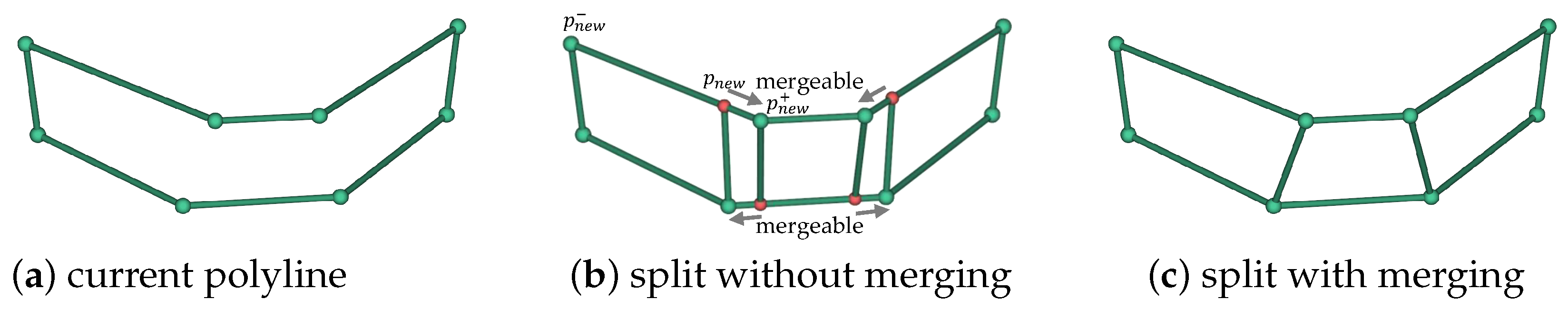
• Our method recursively splits polylines and produces stable results without an ambiguous topology. The merging of new vertices helps avoid unnecessary vertices and keep the compactness of the contours. As shown in the experimental results, our method outperforms by using significantly fewer faces while achieving lower losses compared to other methods.

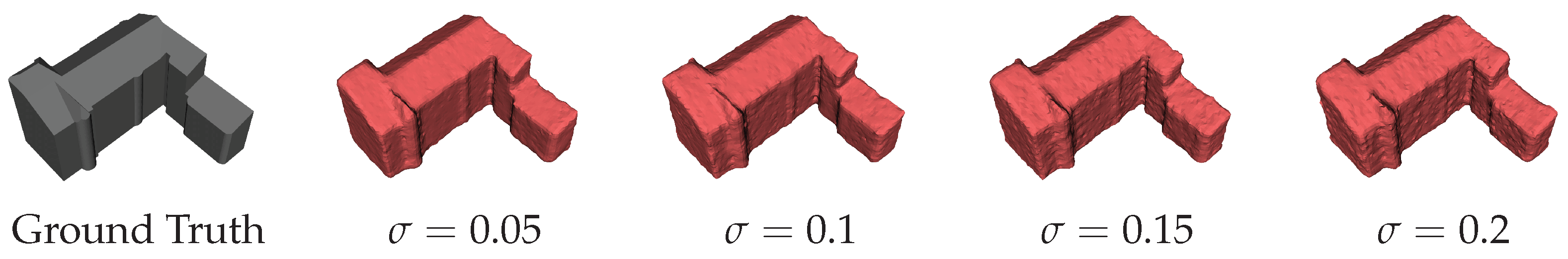
4.3. Effectiveness of Iterative Pipeline

Our method iteratively identifies crucial elevations guided by loss and topological variation to avoid redundant contours. To verify its effectiveness, we compared our iterative method with the evenly spacing strategy. Initially, the building mesh soups used in Section 4.2.1 were reconstructed with default parameters using our iterative method. Subsequently, based on the iterative reconstruction result, two variable-controlled results were generated by the evenly spaced contour-generation strategy for comparison:

• Result 1: Using $n_1$ evenly spaced contour layers. $n_1$ is equal to the number of contour layers in the iterative reconstruction result.
• Result 2: Using $n_2$ evenly spaced contour layers. $n_2$ is the minimum number of contour layers, where the result with $n_2+1$ contour layers has a lower loss than the iterative reconstruction result.

Result 1 has the same number of contour layers as the iterative result, while Result 2 has the same level of loss as the iterative result.

The loss and number of contour layers are summarized and illustrated in Figure 20 and Figure 21. The $\Delta$loss in Figure 20 represents the subtraction of the loss between Result 1 and the corresponding iterative result. Similarly, the $\Delta$layer in Figure 21 represents the subtraction of contour layer count between Result 2 and the corresponding iterative result.

The experimental result shows that our iterative method obtains less loss with the same number of contour layers and, inversely, also uses fewer contour layers to reach the same level of loss. Our iterative method is, thus, demonstrated to possess superior effectiveness compared to the evenly spaced contour-generation strategy.

5. Discussion

5.1. Limitation

Our iterative contour generation method requires a large number of samples to identify the optimal new crucial elevation, which is time-consuming. Another challenge comes from the parameter selection: the target loss of iterative contour generation is difficult to determine due to the variety of building structures. Moreover, reference planes are required in the vertex attaching and corner recovery, but may be absent if the building surface is not planar. In this circumstance, the contour refinement falls back to a traditional polygon simplification method, and corners and details may be lost. Additionally, our contour-interpolation algorithm may fail to generate complex surfaces and require more in-between elevations for the correct surfaces, thus increasing the complexity of the results. Another limitation comes from the limitation of the contours. The contour is difficult to accurately capture topological variations at certain structures such as the top of a pitched roof. For such a roof, a narrow flat roof will be generated with the current method, which is inaccurate.

5.2. Future Work

In our future work, we would like to improve the efficiency of iteration contour generation by strategies such as pre-calculating. To avoid the struggle of parameter selection, auto-fitting parameters could be designed based on the variation trend of the loss. Moreover, to complement the lost information at the top of the pitched roofs, more prior knowledge could be introduced and post-processing could be applied to recover accurate roofs.

6. Conclusions

In this study, we presented a novel iterative contour-based method designed to generate low-poly building meshes with only essential details from mesh soups. Our method is based on an iterative pipeline to extract vital contours near crucial elevations. Low-poly meshes are generated from the vital contours, and then, new vital contours can be extracted by the loss and topological variation of the reconstructed mesh for the next iteration.

Our method focuses on two primary targets for high-quality results: reduce the number of contours and generate compact surfaces between contours. The total number of contours is reduced using our iterative pipeline, as only vital contours are extracted. Moreover, the potential redundant contours are identified and, then, removed based on our contour-interpolation algorithm. With these raw vital contours, compact contours are obtained using our contour refinement method with vertex attaching, corner recovery, and simplification, which takes advantage of the planar primitives of buildings. Additionally, connection relationships between contours are recovered for surface generation using our contour-graph-construction method. Then, our contour-interpolation algorithm is also utilized to generate compact surfaces between connected contours.

Our method imposes no limitation on the input building and exhibits the ability to reconstruct low-poly meshes from mesh soups. The experiments demonstrated that our method generates satisfactory results and has superior effectiveness than previous methods on the quality of the general reconstruction results, contour refinement results, and surface generation results. Additionally, our iterative contour-generation method was demonstrated to outperform the previous evenly spaced contour-generation method in the experiments.

References

- Xu, Y.; Stilla, U. Toward building and civil infrastructure reconstruction from point clouds: A review on data and key techniques. IEEE J. Sel. Top. Appl. Earth Obs. Remote Sens. 2021, 14, 2857–2885. [Google Scholar] [CrossRef]
- Ali, T.; Mehrabian, A. A novel computational paradigm for creating a Triangular Irregular Network (TIN) from LiDAR data. Nonlinear Anal. Theory, Methods Appl. 2009, 71, e624–e629. [Google Scholar] [CrossRef]
- Bouzas, V.; Ledoux, H.; Nan, L. Structure-aware Building Mesh Polygonization. ISPRS J. Photogramm. Remote Sens. 2020, 167, 432–442. [Google Scholar] [CrossRef]
- Gao, X.; Wu, K.; Pan, Z. Low-Poly Mesh Generation for Building Models. In Proceedings of the Special Interest Group on Computer Graphics and Interactive Techniques Conference Proceedings, New York, NY, USA, 7–11 August 2022. [Google Scholar] [CrossRef]
- Li, M.; Nan, L. Feature-preserving 3D mesh simplification for urban buildings. ISPRS J. Photogramm. Remote Sens. 2021, 173, 135–150. [Google Scholar] [CrossRef]
- Huang, J.; Stoter, J.; Peters, R.; Nan, L. City3D: Large-Scale Building Reconstruction from Airborne LiDAR Point Clouds. Remote Sens. 2022, 14, 2254. [Google Scholar] [CrossRef]
- Kamra, V.; Kudeshia, P.; ArabiNaree, S.; Chen, D.; Akiyama, Y.; Peethambaran, J. Lightweight Reconstruction of Urban Buildings: Data Structures, Algorithms, and Future Directions. IEEE J. Sel. Top. Appl. Earth Obs. Remote Sens. 2023, 16, 902–917. [Google Scholar] [CrossRef]
- Zhang, K.; Yan, J.; Chen, S.C. Automatic Construction of Building Footprints From Airborne LIDAR Data. IEEE Trans. Geosci. Remote Sens. 2006, 44, 2523–2533. [Google Scholar] [CrossRef]
- Zhou, Q.Y.; Neumann, U. Fast and Extensible Building Modeling from Airborne LiDAR Data. In Proceedings of the 16th ACM SIGSPATIAL International Conference on Advances in Geographic Information Systems, New York, NY, USA, 5 November 2008. [Google Scholar] [CrossRef]
- Yan, J.; Zhang, K.; Zhang, C.; Chen, S.C.; Narasimhan, G. Automatic Construction of 3-D Building Model From Airborne LIDAR Data Through 2-D Snake Algorithm. IEEE Trans. Geosci. Remote Sens. 2015, 53, 3–14. [Google Scholar] [CrossRef]
- Wang, Y.; Xu, H.; Cheng, L.; Li, M.; Wang, Y.; Xia, N.; Chen, Y.; Tang, Y. Three-Dimensional Reconstruction of Building Roofs from Airborne LiDAR Data Based on a Layer Connection and Smoothness Strategy. Remote Sens. 2016, 8, 415. [Google Scholar] [CrossRef]
- Yan, L.; Li, Y.; Xie, H. Urban Building Mesh Polygonization Based on 1-Ring Patch and Topology Optimization. Remote Sens. 2021, 13, 4777. [Google Scholar] [CrossRef]
- Yan, L.; Li, Y.; Dai, J.; Xie, H. UBMDP: Urban Building Mesh Decoupling and Polygonization. IEEE Trans. Geosci. Remote Sens. 2023, 61, 1–16. [Google Scholar] [CrossRef]
- Zhang, J.; Li, L.; Lu, Q.; Jiang, W. Contour clustering analysis for building reconstruction from LiDAR data. In Proceedings of the International Archives of the Photogrammetry, Remote Sensing and Spatial Information Sciences, Beijing, China, 3–11 July 2008. [Google Scholar]
- Li, L.; Zhang, J.; Jiang, W. Automatic complex building reconstruction from LIDAR based on hierarchical structure analysis. In Proceedings of the MIPPR 2009: Pattern Recognition and Computer Vision, Yichang, China, 30 October–1 November 2009. [Google Scholar] [CrossRef]
- Wu, B.; Yu, B.; Wu, Q.; Yao, S.; Zhao, F.; Mao, W.; Wu, J. A Graph-Based Approach for 3D Building Model Reconstruction from Airborne LiDAR Point Clouds. Remote Sens. 2017, 9, 92. [Google Scholar] [CrossRef]
- Zhang, Y.; Zhang, C.; Chen, S.; Chen, X. Automatic Reconstruction of Building Façade Model from Photogrammetric Mesh Model. Remote Sens. 2021, 13, 3801. [Google Scholar] [CrossRef]
- Zhang, W.; Li, Z.; Shan, J. Optimal Model Fitting for Building Reconstruction From Point Clouds. IEEE J. Sel. Top. Appl. Earth Obs. Remote Sens. 2021, 14, 9636–9650. [Google Scholar] [CrossRef]
- Song, J.; Xia, S.; Wang, J.; Chen, D. Curved Buildings Reconstruction From Airborne LiDAR Data by Matching and Deforming Geometric Primitives. IEEE Trans. Geosci. Remote Sens. 2021, 59, 1660–1674. [Google Scholar] [CrossRef]
- Coiffier, G.; Basselin, J.; Ray, N.; Sokolov, D. Parametric Surface Fitting on Airborne Lidar Point Clouds for Building Reconstruction. Comput. Aided Des. 2021, 140, 103090. [Google Scholar] [CrossRef]
- Qian, Y.; Zhang, H.; Furukawa, Y. Roof-GAN: Learning To Generate Roof Geometry and Relations for Residential Houses. In Proceedings of the 2021 IEEE/CVF Conference on Computer Vision and Pattern Recognition (CVPR), Nashville, TN, USA, 20–25 June 2021. [Google Scholar] [CrossRef]
- Li, M.; Wonka, P.; Nan, L. Manhattan-world Urban Reconstruction from Point Clouds. In Proceedings of the European Conference on Computer Vision, Amsterdam, The Netherlands, 11–14 October 2016. [Google Scholar] [CrossRef]
- Nan, L.; Wonka, P. PolyFit: Polygonal Surface Reconstruction from Point Clouds. In Proceedings of the 2017 IEEE International Conference on Computer Vision (ICCV), Venice, Italy, 22–29 October 2017. [Google Scholar] [CrossRef]
- Liu, X.; Zhang, Y.; Ling, X.; Wan, Y.; Liu, L.; Li, Q. TopoLAP: Topology Recovery for Building Reconstruction by Deducing the Relationships between Linear and Planar Primitives. Remote Sens. 2019, 11, 1372. [Google Scholar] [CrossRef]
- Xie, L.; Hu, H.; Zhu, Q.; Li, X.; Tang, S.; Li, Y.; Guo, R.; Zhang, Y.; Wang, W. Combined Rule-Based and Hypothesis-Based Method for Building Model Reconstruction from Photogrammetric Point Clouds. Remote Sens. 2021, 13, 1107. [Google Scholar] [CrossRef]
- Chen, Z.; Ledoux, H.; Khademi, S.; Nan, L. Reconstructing compact building models from point clouds using deep implicit fields. ISPRS J. Photogramm. Remote Sens. 2022, 194, 58–73. [Google Scholar] [CrossRef]
- Garland, M.; Heckbert, P.S. Surface simplification using quadric error metrics. In Proceedings of the SIGGRAPH97: The 24th International Conference on Computer Graphics and Interactive Techniques, New York, NY, USA, 3 August 1997. [Google Scholar] [CrossRef]
- Wang, S.; Liu, X.; Zhang, Y.; Li, J.; Zou, S.; Wu, J.; Tao, C.; Liu, Q.; Cai, G. Semantic-guided 3D building reconstruction from triangle meshes. Int. J. Appl. Earth Obs. Geoinf. 2023, 119, 103324. [Google Scholar] [CrossRef]
- Heckbert, P.S.; Garland, M. Survey of Polygonal Surface Simplification Algorithms; Technical Report; School of Computer Science, Carnegie Mellon University: Pittsburgh, PA, USA, 1997. [Google Scholar]
- Wu, Q.; Liu, H.; Wang, S.; Yu, B.; Beck, R.; Hinkel, K. A Localized Contour Tree Method for Deriving Geometric and Topological Properties of Complex Surface Depressions Based on High-Resolution Topographical Data. Int. J. Geogr. Inf. Sci. 2015, 29, 2041–2060. [Google Scholar] [CrossRef]
- Wu, B.; Yu, B.; Wu, Q.; Huang, Y.; Chen, Z.; Wu, J. Individual Tree Crown Delineation Using Localized Contour Tree Method and Airborne LiDAR Data in Coniferous Forests. Int. J. Appl. Earth Obs. Geoinf. 2016, 52, 82–94. [Google Scholar] [CrossRef]
- Helsingin Kaupungin Kaupunginkanslia, t.j.v. 3D Models of Helsinki. Available online: https://hri.fi/data/en_GB/dataset/helsingin-3d-kaupunkimalli (accessed on 7 December 2023).