Abstract
The technology of infrared dim- and small-target detection is irreplaceable in many fields, such as those of missile early warning systems and forest fire prevention, among others. However, numerous components interfere with infrared imaging, presenting challenges for achieving successful detection of infrared dim and small targets with a low rate of false alarms. Hence, we propose a new infrared dim- and small-target detection network, Multiscale Feature Extraction U-Net for Infrared Dim- and Small-Target Detection (MFEU-Net), which can accurately detect targets in complex backgrounds. It uses the U-Net structure, and the encoders and decoders consist of ReSidual U-block and Inception, allowing rich multiscale feature information to be extracted. Thus, the effectiveness of algorithms in detecting very small-sized targets can be improved. In addition, through the multidimensional channel and spatial attention mechanism, the model can be adjusted to focus more on the target area in the image, improving its extraction of target information and detection performance in different scenarios. The experimental results show that our proposed algorithm outperforms other advanced algorithms in detection performance. On the MFIRST, SIRST, and IRSTD-1k datasets, we achieved detection rates of 0.864, 0.962, and 0.965; IoU values of 0.514, 0.671, and 0.630; and false alarm rates of 3.08 × , 2.61 × , and 1.81 × , respectively.
1. Introduction
Infrared detection systems can distinguish between a target and its background by collecting the different radiation signatures and comparing between the two. They are a type of passive detection system able to work under all-weather conditions without being influenced by light and can realize long-distance detection with high detection accuracy. As they are not affected by the shortcoming of interference from other electromagnetic waves, in contrast to detection based on radar and visible light, they have become one of the important means of acquiring strategic perception data, experiencing very high application in both military and civil contexts [1]. However, in practical applications, such as involving guidance, early-warning, airborne, or satellite surveillance, the very long distance of targets from the detector results in them representing a very small percentage of the image output from the detector; at the same time, such targets are generally not the brightest in the image due to the effect of atmospheric scattering and absorption, and this kind of typical target is usually referred to as an infrared dim and small target (IDST) [2].
IDSTs usually present as a speckle in the image, thus lacking geometrical and textural feature information, and the target is often submerged in the background, which makes it impossible to extract the target through global grayscale characteristics [3]. Compared with sky and sea backgrounds, ground backgrounds are more complex, and there are often sources of interference, such as noise and small edges, close to the IDST in the background, which will lead to a more complex and variable grayscale distribution in the target neighborhood. All these factors lead to IDSTs being difficult to detect. Therefore, IDST detection represents both a difficulty and a hotspot in the field of target detection. The ability to function under real-time detection conditions is an important application requirement in the practical projects of detection algorithms, which have high research and application value in many fields [4].
Numerous traditional target detection algorithms have previously been proposed by researchers [5]. Filter-based methods use a specific filter that can eliminate the background of the infrared image to detect the IDST. Filter-based methods require less computation but have low efficacy. They can thus only be used in specific scenes to suppress the background of a gentle change and cannot solve the problem of complex background [6]. The LCM-based methods take advantage of the difference in gray values between the target and the background to boost the gray values of the target while reducing those of the background, but good detection results can mostly only be obtained when there is high image contrast, so the algorithm’s generalization ability is poor, and it cannot be effectively applied to complex backgrounds [7]. Data structure-based methods mainly transform the IDST detection problem into a convex optimization problem with low-rank and sparse matrix recovery. This type of algorithm has good applicability to images with complex backgrounds. However, the algorithm is very computationally intensive, so it is not suitable for imaging in real-time applications where latency is significantly compromised [8].
Due to the many advantages of deep learning-based algorithms, numerous researchers have proposed their use in IDST detection [9]. Since the size of an IDST is very small, and they are very sensitive to bounding box perturbation, image segmentation methods are adopted in most approaches for IDST detection such that more fine target information can be obtained [10]. In order to detect very-small-size and general-size targets, some algorithms enhance the information fusion between different layers so they can extract the information for different sizes and improve the detection effect for differently sized targets [11]. Due to the sparse nature of IDSTs, some algorithms enhance the visibility of targets by suppressing the background [12]. There are also algorithms that use GAN networks to separately address the problem of missed and false alarms, using different generators to address the difficult balance between them [13].
The existing IDST detection algorithms still have some limitations. The traditional methods are overly dependent on a priori knowledge and have poor detection performance in real scenes [14]. Although the above deep learning algorithms have achieved good detection results, most cannot achieve a good balance between the detection rate and the false alarm rate. In addition, some algorithms with insufficient generalization ability can only be used with specific datasets and cannot meet the requirements for real-scene detection [15].
In this paper, we propose a new convolutional network-based system for IDST detection: the Multiscale Feature Extraction U-Net for Infrared Dim- and Small-Target Detection (MFEU-net). The network uses U-Net, and ReSidual U-block (RSU) and Inception modules are introduced in the encoders and decoders to extract multiscale feature information, making it possible to detect very small IDSTs. There are multidimensional channels and spatial attention mechanisms in each encoder and decoder, and the global information is extracted by the attention mechanism such that the model can give a greater weight to the target area, thereby improving the ability of the model to adapt to different scenarios as well as the detection performance with complex backgrounds. The algorithm proposed in this paper has the lowest leakage detection rates and false alarm rates.
Overall, the main contributions of this paper are as follows:
(1) We design a multiscale feature extraction network using a combination of ReSidual U-block (RSU) and Inception, which enables the network to have different receptive fields at one level, allowing the network to adapt to scenarios containing targets of different sizes;
(2) We design a multidimensional channel and spatial attention mechanism (MCSAM) that can make full use of the different information in the feature map and more effectively determine the region where the target is located;
(3) Compared to other state-of-the-art algorithms, our algorithm achieved better detection results on different datasets.
2. Materials and Methods
2.1. Related Work
2.1.1. IDST Detection
Traditional single-frame IDST detection methods can be divided into filter-based methods, local contrast measure (LCM)-based methods, and data structure-based methods.
Filter-based methods can be divided into spatial- and transform-domain filtering. In the spatial-domain filtering methods, a specific filtering kernel is used to remove the background in the infrared image [16]. For these methods, start by designing a filter kernel based on the characteristics of the background and the target to eliminate the background, then use the estimated background to perform a difference operation with the original image, and finally threshold the difference image to segment and detect IDSTs. With the frequency-domain filtering approach, the background is considered to be low frequency and the target to be high frequency, and by designing an appropriate high-pass filter, the low-frequency background and the high-frequency target can be separated [17]. Overall, filtering-based methods require less computation but have low efficacy, being only applicable to scenes with very little background change. Thus, they cannot be used to solve the problem of complex backgrounds and, moreover, have high false alarm rates and poor algorithm robustness [18].
The LCM-based algorithm uses the different gray values of the target images and other images to calculate different gain factors such that the difference between the two can be increased, making the target more prominent [19]. In the LCM approach, a kernel is used to traverse the entire image, multiplying the gray value at the center of the kernel by the ratio of the center gray value to the average gray value of the surrounding area, and when the center gray value of the kernel greatly exceeds the surrounding gray value, the center of the kernel is considered to be the target, and a saliency map can be obtained. Then, the small targets are segmented in the saliency map via thresholding. Finally, the position of the targets in the saliency map must correspond to the original image to achieve IDST detection [20]. The key to this algorithm is the way in which the saliency map is acquired, which will greatly affect the algorithm’s performance. These LCM-based methods can be used to suppress background enhancement targets through certain means, but most them can only detect targets when there is high image contrast, and the generalization ability of the algorithm is poor, so it cannot be effectively applied to complex backgrounds [21].
The methods based on image data structure involve transforming the small-target detection problem into a convex optimization problem for low-rank and sparse matrix restoration based on the sparsity of the target and the low rank of the background [22]. These algorithms are based on the two prerequisites of having few targets and strong background correlation in infrared images, so when these two conditions are not met, these algorithms are much less effective in detection. The methods based on image data structure have good applicability for images with fewer targets and complex backgrounds, but these algorithms will have leakage detection in the case of more targets, and the computational weight is very high, so they are difficult to apply to remote sensing images [23].
Deep learning algorithms can realize complex nonlinear computations and surpass traditional algorithms in many areas, so they are increasingly being applied in IDST detection [24].
Wang et al. used two independent generators, each accomplishing the task of reducing false alarms and missed detections, and the two models were based on a contextual aggregation network that could utilize different feature information, thus achieving low rates of missed detections and false alarms in IDST detection [25]. In addition, they published a large synthetic IDST detection dataset that can be used in advancing the development of IDST detection algorithms.
Lee et al. incorporated fusion and augmentation modules at each level of the network, and through repeated augmentation and fusion, different levels of information could be fused to retain more information about the target [26]. However, it was necessary to retain many of the previous feature maps, thereby consuming high amounts of storage resources, which poses a problem for practical use.
Chen et al. designed a global attention mechanism that can be used to separately extract local and global features, eliminate most of the background pixels, and highlight the target location; by fusing global and local features, the target can be detected using multiscale information [27]. However, its post-processing is complex, blurring the target with loss of detailed information.
Hou et al. utilized ResNet to extract features in the form of groups, making it possible increase the weight of important groups; furthermore, the addition of a fully connected layer to the jump connections of U-Net allows the network to extract global information to improve target extraction [28]. However, the use of the mean square error (MSE) as a loss function results in the network being prone to predicting the target as background during training due to the imbalance in positive and negative samples.
Yu et al. proposed a multiscale local contrast learning mechanism, which can generate multiscale local contrast feature maps during the training process such that more detailed information about the target can be extracted, enabling the network to better localize the target position [29]. However, the use of normal convolutional layers and dilation convolution to extract local information introduces a grid effect when the dilation parameter is excessively large, which tends to result in the loss of target information.
2.1.2. Attention Mechanism
In deep learning, an attention mechanism (AM) can be used to ensure neural networks prioritize important regions when processing data by mimicking the human visual and cognitive systems and adding different weights to different regions in the feature map [30]. By introducing an attention mechanism, different regions of the input feature map can be multiplied by different weighting factors, and the neural network is able to focus on important local information from the global information and more important information can be extracted by the network such that the model can make more accurate predictions or classifications without consuming more computational and storage resources. Therefore, AMs have been widely used in deep learning networks, such as SE-Net, ECA-Net, CBAM, etc. [31].
Squeeze-and-Excitation Networks (SE-Nets) [32] are representative of work in the field of CV where the attention mechanism is applied to the channel dimension. They have a simple and effective structure and can adaptively adjust the feature responses between channels by means of feature recalibration. This network extracts global information using the global average pooling operation and downsamples all feature maps to a single point. After that, it utilizes a two-layer multilayer perceptron network to change the weights of different regions. The sigmoid activation function is then used to generate the channel weights, after which the Hadamard product is computed with the input to obtain the channel-weighted feature map.
Efficient Channel Attention (ECA-Net) [33] is an improvement of the feature transformation part of SE-Nets. The channel information interaction of SE-Nets is realized through the full connection, which damages a part of the feature expression in the process of downscaling and upscaling, while ECA-Net utilizes one-dimensional convolution to realize channel information interaction, which significantly reduces the computational complexity, basically with no loss of performance.
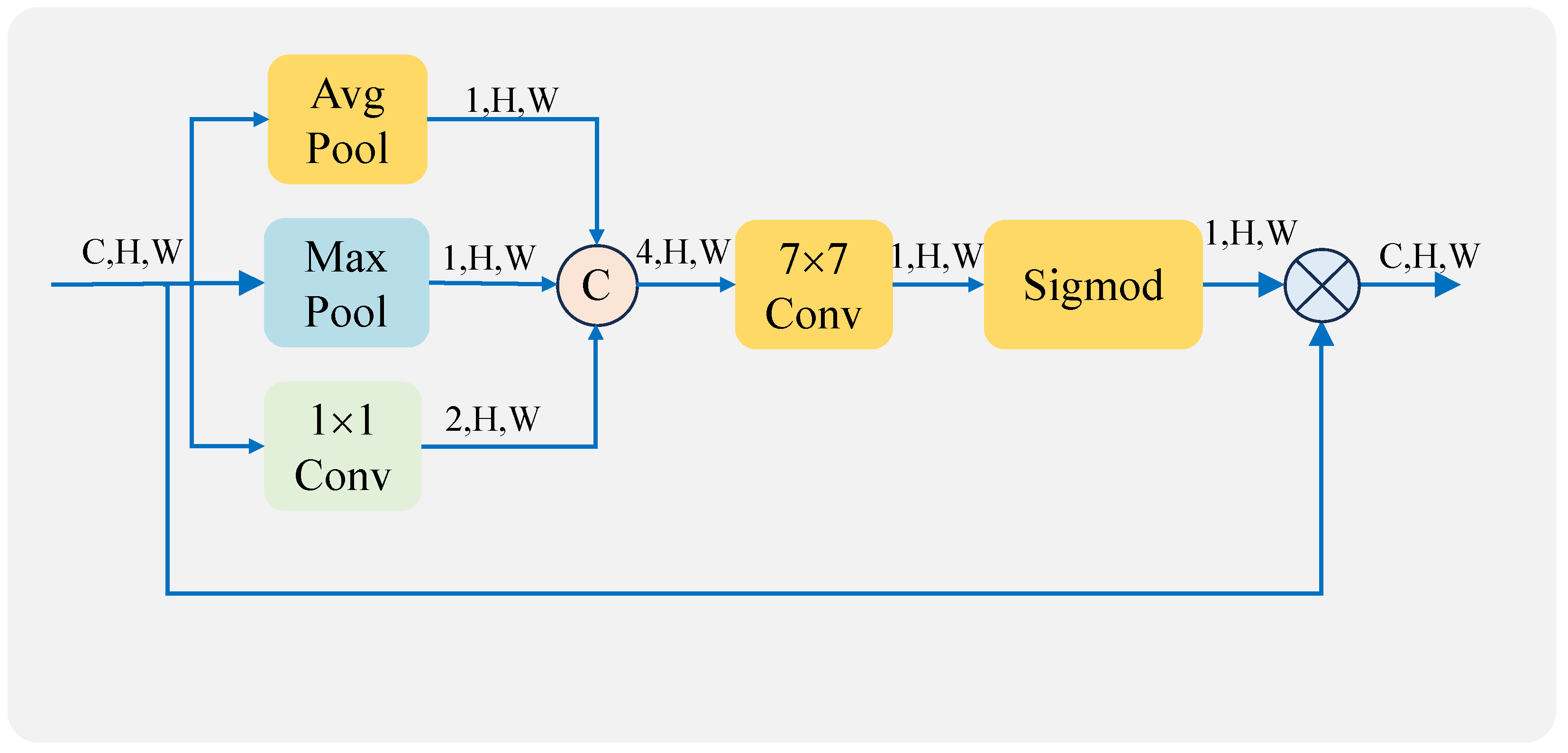
The Convolutional Block Attention Module (CBAM) [34] can be understood as adding a spatial attention module (SAM) to an SE-Net, which separately calculates weights in the channel and spatial domains, allowing it to more precisely localize the region where the target is located compared to a single-channel attention mechanism. A SAM generates two feature maps containing different global information through two pooling operations, which are concatenated together and then fused by a -sized convolutional layer. Finally, a sigmoid operation is performed to generate a weight map, after which the Hadamard product is computed from the original input feature map to enhance the target region.
2.2. Method
2.2.1. Overall Architecture
U-Net can fuse different information at different levels through skip connections such that detailed information at the low level can be directly passed to the high level, thus providing richer contextual and detailed information. This skip connection design helps the network to better capture the boundaries and details of the target and results in improved accuracy of detection. Another advantage of U-Net is its efficient architectural design, especially the skip connections and symmetric expansion paths, which contribute to the network’s good performance even on small datasets. Thus, we use the U-Net structure in our deep learning network.
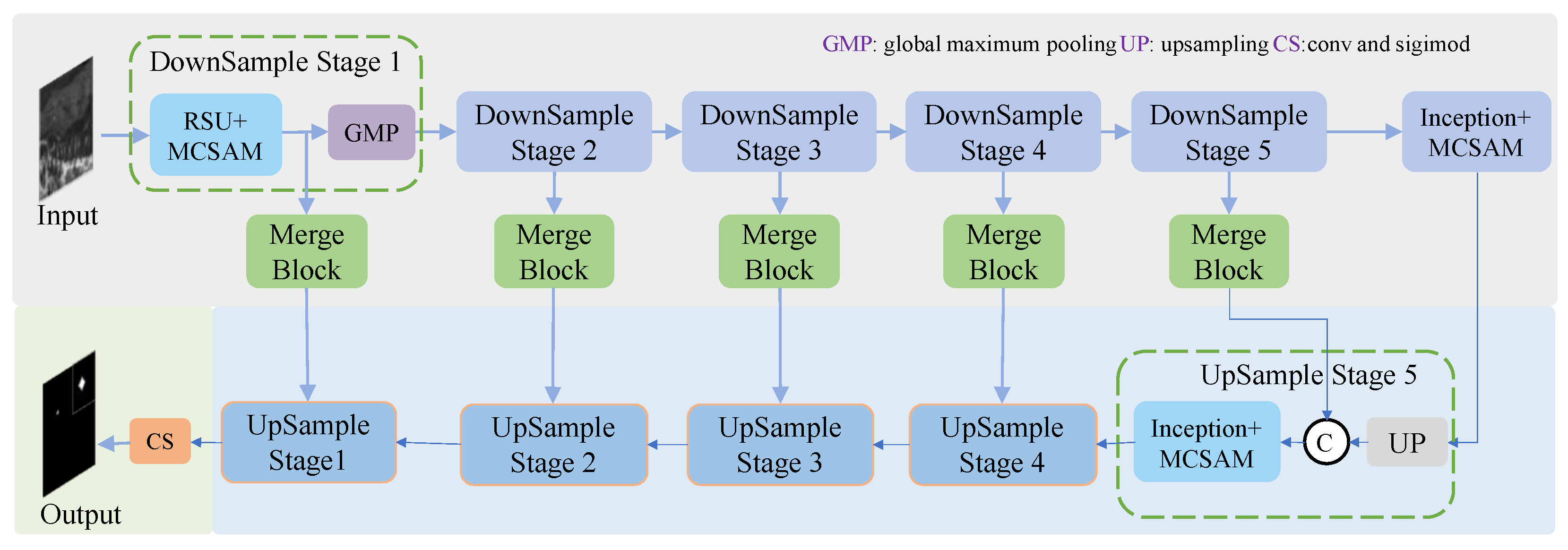
Structurally, the upsampling stage and the downsampling stage are basically symmetrical. The downsampling stage consists of an encoder module and global maximum pooling for extracting the multiscale information of the input feature maps and downsampling the feature maps. The upsampling phase consists of an upsampling and decoder module in which linear interpolation is used to upsample the low-resolution feature map, and the multiscale information from different layers is then fused. In stages one to four, the encoder and decoder are RSU and MCSAM, while in stages five to six, the encoder and decoder are Inception and MCSAM. The downsampling stage and the upsampling stage are connected by the Merge module. The structure of MFEU-Net is shown in Figure 1.
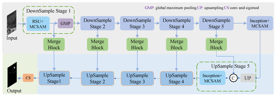
Figure 1.
MFEU-Net structure.
Inside the Merge module is a ResNet consisting of convolutional layers with a convolutional kernel size of . Through these convolutional layers, the information of different channels can be fused, and the nonlinear ability of the model can be increased after convolution through the activation function.
2.2.2. Encoder and Decoder
Conventional convolutional layers have a fixed convolutional kernel size, which means they have a fixed sense field for the input image. Therefore, they cannot fully utilize the contextual information and have poor detection performance when encountering very small targets. Multiscale feature extraction methods can enable a network to have different receptive field sizes at different layers by adding parallel convolutional branches or using pooling operations at different scales. Thus, they enable the algorithm to better detect very small targets in the image.
ReSidual U-block (RSU) [35] uses small U-Net modules instead of single-stream convolution, so it can have a variety of different-sized receptive fields at different layers, which allows it to better capture contextual information at different scales. RSU uses pooling operations to increase the overall architecture depth as well as the network’s ability to sense global and semantic information through multiple downsampling.
However, excessive downsampling will lead to a large reduction in detail information, and u-sampling will bring invalid information when concatenating with high-resolution feature maps, affecting the retention of detail information. In addition, U-Net’s structure is dependent on retention of the feature maps before downsampling, and multiple rounds of downsampling will increase the number of feature maps to be retained, which will consume a large amount of storage resources. For this reason, we reduce the number of downsampling events in the RSU module and remove the feature maps that will not subsequently be used. As a result, more information in the feature map can be retained, and the consumption of storage resources is reduced.
Inception uses parallel convolution and pooling operations of different sizes or different depths to capture rich multiscale information, allowing the model to handle richer spatial features and increase feature diversity [36]. Inception modules can be repeatedly stacked to form larger networks, which can effectively extend the depth and width of the network, preventing overfitting phenomena while improving the accuracy of deep learning networks. However, for parallel multibranching, a large number of parameters are introduced to the model, increasing the requirement for computational resources and the time for training and inference. Therefore, we decrease the parameters by reducing the number of channels in each branch.
Therefore, a combination of RSU and Inception is used such that the U-Net has different multiscale features at different levels. In the initial stage, RSU is used and the amount of downsampling is limited. Its structure is shown in Figure 2. First, the number of channels of the input feature map is changed by a convolutional layer of size . The data are then fed into the RSU module. In the RSU there is a small U-Net, whose encoder and decoder employ ResNet and are connected by skip connections. The data are then fed into the AM to add different weights to different regions of the feature map. Finally, they data are added to the feature map after changing the number of channels and output to the next module.

Figure 2.
Architecture diagram of an encoder and decoder using the RSU module.
By changing the number of downsampling events, the depth of the RSU module can be changed to accommodate different-sized feature maps. Specifically, encoder and decoder block one uses four rounds of downsampling, encoder and decoder block two uses three rounds of downsampling, encoder and decoder block three uses two rounds of downsampling, and encoder and decoder block four uses one round of downsampling.
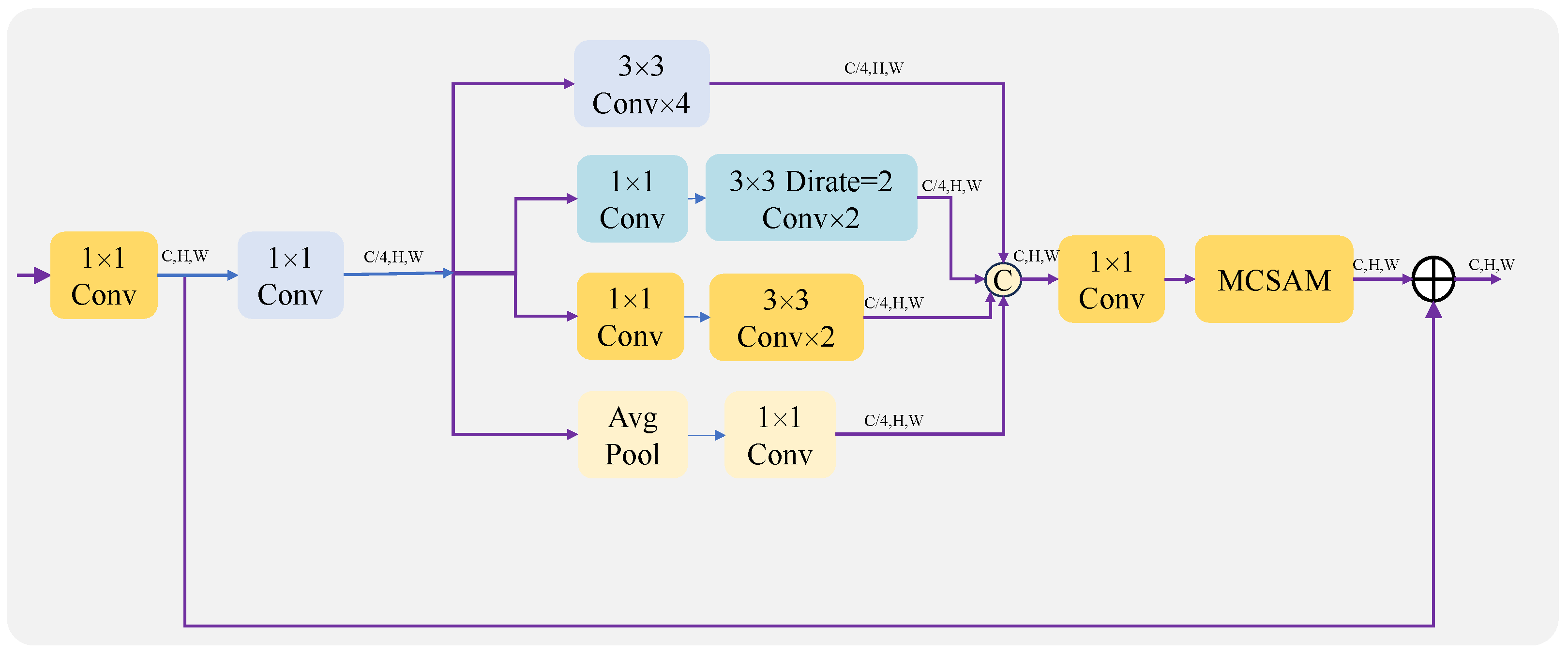
Following this, Inception is used. In order to avoid having excessive parameters, four different branches are used, and the number of channels in each branch is one-quarter of the number of output channels. Since the parameters of the convolutional layer are proportional to the square of the number of channels, the parameters and computation of the model can be drastically reduced by reducing the number of channels. Its structure is shown in Figure 3. First, the number of channels of the input feature map is changed to the number of output channels by a convolutional layer of size . It is then fed into four different branches.
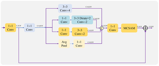
Figure 3.
Architecture diagram of an encoder and decoder using Inception.
Through different branches, different examples of feature information can be learned and synthesized to improve model performance. Afterwards, the outputs of these four different branches are concatenated together and fed into a -sized convolutional layer, exchanging information between the different channels. The output is then fed into the AM to add different weights to different regions of the feature map. Finally, it is added to the feature map after changing the number of channels and output to the next module.
The backbone network and the number of downsampling events at different stages are shown in Table 1. This allows the model to have different receptive fields without significantly increasing the number of model parameters, resulting in improving the efficacy of IDST detection.

Table 1.
Backbone network and number of rounds of downsampling at different stages.
2.2.3. Attention Mechanism
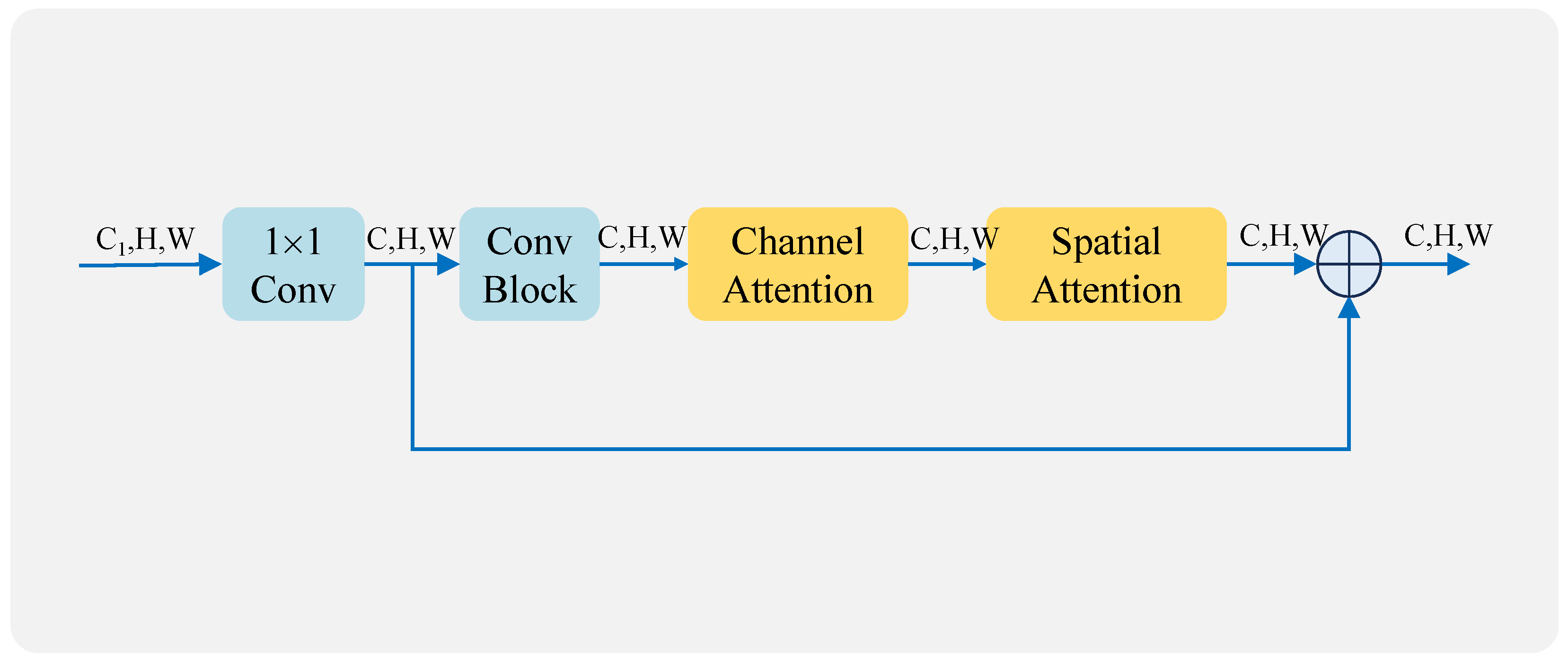
In this section, we describe the design of a Multidimensional Channel Attention and Spatial Attention Mechanism (MCSAM) to extract global information. Through the attention mechanism, more weight can be given to the focus area in the feature map. The channel AM is first utilized to generate different weights for each channel in its channel domain for the input feature map. Then, the spatial AM is utilized to generate different weights for each region in the spatial domain for the channel-weighted feature maps. The structure diagram is shown in Figure 4.
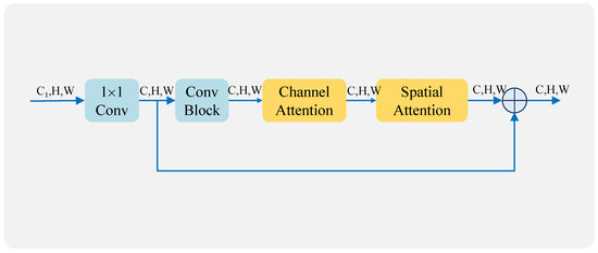
Figure 4.
MCSAM structure.
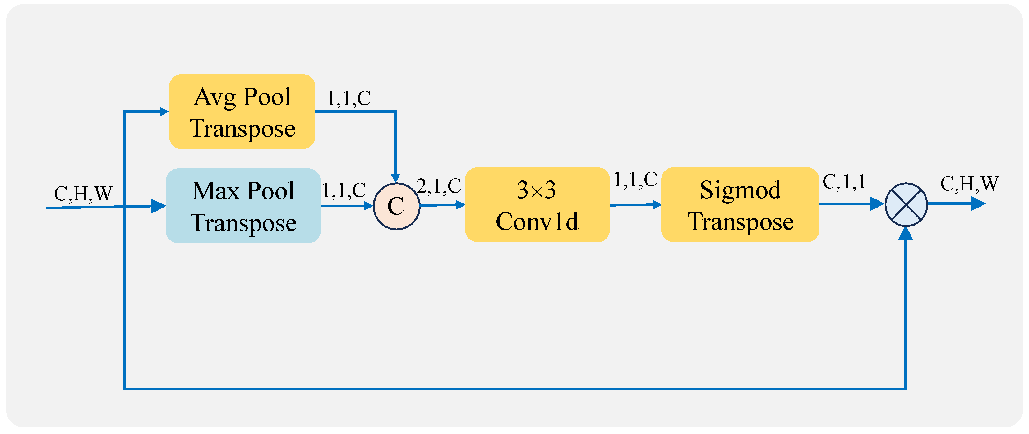
In the channel attention mechanism, to extract more advanced information, we additionally add pooling operations. Two feature maps () are generated by performing global maximum pooling () and global average pooling () on the input feature maps (F). The two feature maps are concatenated on the channel domain to obtain a feature map. After that, a feature map is generated by one-dimensional convolution. A channel weight feature map () is then obtained by using the sigmoid function () and transpose operation on it. Finally, the Hadamard product (⊗) is computed using the input feature map to get a channel-weighted feature map. The process is illustrated in Equation 1. The structure diagram is shown in Figure 5.
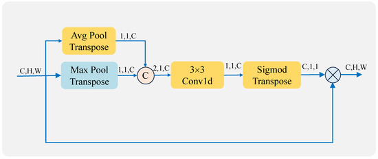
Figure 5.
Channel attention structure.
SAM extracts information using only pooling operations, which can result in a significant loss of local information. In order to retain more information, we additionally add a convolution operation that can retain feature information differently from the pooling retention operation. This is beneficial in generating better spatial weights and enabling the model to better localize the target.
The feature maps (F) are fed into the spatial attention mechanism, which first generates feature maps () of sizes , , and using global average pooling (), global maximum pooling (), and a convolutional layer () of size , respectively. Through the convolution and pooling operations, different features can be extracted and more information can be retained. These feature maps are then concatenated together and fed into a convolutional layer (Conv) of size to fuse different types of feature information. After that, the spatial weights () are generated using the sigmod function (), and then the Hadamard product (⊗) is computed using the input feature map to generate a spatially weighted feature map () [34]. The process is illustrated in Equation (2). The structure diagram is shown in Figure 6.
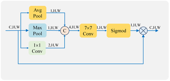
Figure 6.
Spatial attention structure.
MCSAM uses channel and spatial attention in tandem, where the input feature maps (F) are first fed into the channel attention mechanism to generate channel-weighted feature maps () and later into the spatial attention mechanism to generate spatially weighted feature maps (). The formula for the entire MCSAM is shown in Equation (3). By varying the parameters of the convolutional layer, the weights generated by the attention mechanism can be changed and therefore increase the visibility of the area containing the image, thereby improving the perception and discrimination abilities of the model.
2.2.4. Loss Function
Due to the small sizes and low numbers of IDSTs, they comprise only a small portion of an image, and the sum of target pixels as positive samples is much less than the sum of background pixels as negative samples. Therefore, when using infrared images to train the model, there is a very serious imbalance in positive and negative samples, which leads to a decrease in the model’s ability to recognize the target category, and it can easily misclassify the target as background.
For this reason, we use the sum of focal loss and dice loss as the loss function of the algorithm. When calculating the value of the loss function, different weights are separately added for different samples such that each of these samples have a roughly equal share in the loss function during training. As a result, the model can learn the different features of different samples simultaneously in becoming fully trained, thus reducing the possibility of the algorithm predicting all samples as negative.
Dice loss (DL) [37] is a region-dependent loss function, where the value of the loss function is independent of the whole image and is related only to the intersection and concatenation of the actual and predicted target regions. The formula for DL is shown in Equation (4):
Here, TP represents true positive, FP represents false positive, FN represents false negative, and s takes the value 1 × to avoid having a denominator of 0.
Focal loss (FL) [38] is a loss function specialized in solving the problem of too many negative samples in the training data. The formula for FL is shown in Equation (5).
where is an adjustable balancing parameter that regulates the proportion of different samples in the loss function. is a regulatory factor used to control the weight difference between samples that are easy to classify and those that are difficult to classify. p represents the prediction probability, wherein the closer p is to 0 or 1, the easier it is to categorize. y is the true labeling, where 1 indicates the target and 0 indicates the background.
DL focuses on the overall target, while FL focuses on individual pixels, so the final loss function is
3. Results
3.1. Evaluation Metrics
The probability of detection () and false alarm rate () were used to assess whether the algorithm can accurately detect the target, and IoU was used to estimate whether the algorithm can retain the shape of the target. For these three metrics, we used a fixed threshold of . In addition, ROC curves were used to evaluate whether the algorithm can accurately detect the target under dynamic thresholds [39].
Probability of detection () reflects the ability to correctly detect targets and is the ratio of the sum of correctly detected targets to the actual sum of targets . Its formula is shown in Equation (7):
The false alarm rate () reflects the accuracy of the algorithm in detecting the target and is the ratio of the sum of false predicted pixels to the sum of pixels in the whole image . It is defined by the formula shown in Equation (8):
IoU reflects the degree of shape resemblance between the predicted and actual targets and is the ratio of the intersection and union of the two (intersection/union of the two). It takes a value between 0 and 1, where 0 means there is no overlap at all, and 1 means there is perfect overlap. The calculation formula is
where TP represents true positive, FP represents false positive, and FN represents false negative.
The ROC curve represents the classification effect of a classifier under different thresholds; specifically, the curve from left to right can be thought of as a change in threshold from 0 to 1. Its vertical axis is the true positive rate (TPR) and its horizontal axis is the false positive rate (FPR). The closer the curve is to the coordinates (0, 1), the better the performance of the algorithm. The TPR and FPR are calculated as follows:
where N is the sum of pixels in the whole image, TP represents true positive, and FP represents false positive.
3.2. Implementation Details
For the proposed network MFEU-Net, we performed ablation experiments and comparisons with other algorithms using three publicly available datasets: SIRST [40], MFIRST [25], IRSTD-1k [41]. We used an NVIDIA RTX A6000 (48 GB memory) for our graphics cards, and the algorithms were all based on a Pytorch neural network framework.
The training set image size of MFIRST is , and the batch size (BS) can be up to 128 on the A6000, but in order to avoid it being too large such that it would negatively impact the model, we set the BS to 32, the epoch to 100, and the learning rate (LR) to 1 × . The test set image size of MFIRST is not fixed, so we set the BS as 1.
There are 427 images in the SIRST dataset, which is separated into a training set and a test set with 332 and 85 images, respectively. The image size is not fixed in the SIRST data, so we resized all the images in the training set to , and the size of the images in the test set was kept unchanged. For training, we set the BS, epoch, and LR to 8, 100, and 1 × , respectively. For testing, the BS was 1.
There are 1001 images in the IRSTD-1k dataset, which is separated into a training set and a test set with 901 and 100 images, respectively. The image sizes in the SIRST data are all . For the training, we set the BS, epoch, and LR to 8, 100, and 1 × , respectively. For testing, the BS was 8.
3.3. Ablation Study
To validate the effectiveness of our proposed algorithm, we performed an ablation experiment on the aforementioned dataset. Specifically, the performance of networks using different backbones was compared with the overall structure unmodified, and the performance of networks with and without the attention mechanism was compared with all other structures unchanged. For each comparison experiment, we ensured that the structure of the other parts remained the same.
3.3.1. Different Backbones
We compared the detection performance of networks using classical residual networks and networks using RSU without Reduced Downsampling Times (RSURD). A comparison of their specific performance metrics is shown in Table 2. It can be found that the of MFEU-Net was higher than that of the network using RSURD, while the of the network using RSURD was higher than that of the network using ResNet. Our proposed multiscale feature extraction network can extract rich multiscale information, and our algorithm can retain more detail for this information compared with RSURD, thereby outperforming RSURD in different quantitative metrics. Compared with the single-stream ResNet, the detection effect of the model can be substantially improved by multiscale feature extraction. MFEU-Net achieved the highest and the lowest , which demonstrates that our proposed backbone network of RSU combined with Inception is able to extract more information about different features, enabling the model to detect targets of different sizes in different scenarios.

Table 2.
Comparison of quantitative metrics for the different backbone networks. The best of these metrics are shown in red bold font.
3.3.2. Attention Mechanism
We compared the detection performance of networks without and using MCSAM, and the specific indicators are shown in Table 3. It is obvious from the different evaluation metrics that the networks that used attention mechanisms outperformed those that did not. The above analysis clearly demonstrates that our proposed MCSAM can effectively determine the IDST location, which demonstrates the necessity of introducing MCSAM.

Table 3.
Comparison of detection performance of the different backbone networks.The best of these metrics are shown in red bold font.
3.4. Comparison to State-of-the-Art Methods
We selected different algorithms for comparison, including Infrared Patch Image (IPI) [42], MPCM [21], FKRW [43], MDvsFA cGAN (MDFA) [25], Dense Nested Attention Network (DNA) [26], Infrared Small Target Detection U-Net (ISTDU) [28], Local Patch Network with Global Attention (LPNet) [27], and Multiscale Local Contrast Learning (MLCL) networks [29].
3.4.1. Quantitative Comparison
The quantitative metrics for these algorithms are shown in Table 4. The best of these quantitative metrics are shown in red bolded font and the second best in blue font. Overall, thanks to the feature representation capability, the quantization metrics for the deep learning-based algorithms were significantly higher than the traditional algorithms.

Table 4.
Comparison of quantitative metrics for the different algorithms on different datasets. The best of these metrics are shown in red bold font, and the second-best metrics are shown in blue font.
The MPCM algorithm is very sensitive to edges and drastic grayscale changes, so it could detect most of the targets and had a high ; however, it also had a high , one of the highest among the evaluated algorithms. The FKRW algorithm removes the edges and noise in an image but also part of the detail information, so the of this algorithm was relatively low. The IPI algorithm achieved better and compared to the other two conventional algorithms. However, its detection efficacy depends on the sparsity of the targets, which is affected when there are multiple targets in the image. This is also illustrated by the fact that the IPI algorithm did not achieve as good a in the IRSTD-1k dataset as in the other two datasets.
ISTDU groups feature maps and enhances the weights of IDST feature map groups to improve IDST characterization, but it uses the mean squared error (MSE) as the loss function, and due to the imbalance between positive and negative samples, it tends to predict the target as background, so its detection rate was not very high. DNA can make full use of contextual information through a large number of jump connections, but it does not have an attention mechanism, so its detection performance was not very good. MDFA uses two generators responsible for the and , respectively, and its was very high. However, its network is relatively simple and cannot adapt to complex scenarios, and its was also high. MLCL uses a combination of convolutional-layer and dilated-convolutional-layer approaches to learn local contrast feature information, but the dilation is too large to lead to the grid effect, resulting in the target being easily lost, so its detection rate was very low. LPNet can extract global and local information at the same time, which can improve the detection effect of the algorithm, but the target becomes fuzzy in post-processing, so the IoU was not high.
The deep learning algorithms proposed in this paper outperformed the other methods. The proposed algorithm achieved the lowest , highest IoU, and high on the MFIRST dataset. It also achieved the best , , and IoU on the SIRST and IRSTD-1k datasets. Our algorithm also outperformed others in terms of ROC curves on different datasets, as shown in Figure 7. Taken together, our algorithm outperformed the other algorithms.

Figure 7.
ROC curves of different algorithms. The ROC performance of IPI and MPCM was too poor to be shown in the figure. (a) ROC curves of different algorithms with the MFIRST dataset. (b) ROC curves of different algorithms with the SIRST dataset. (c) ROC curves of different algorithms with the IRSTD-1k dataset.
3.4.2. Visual Comparison
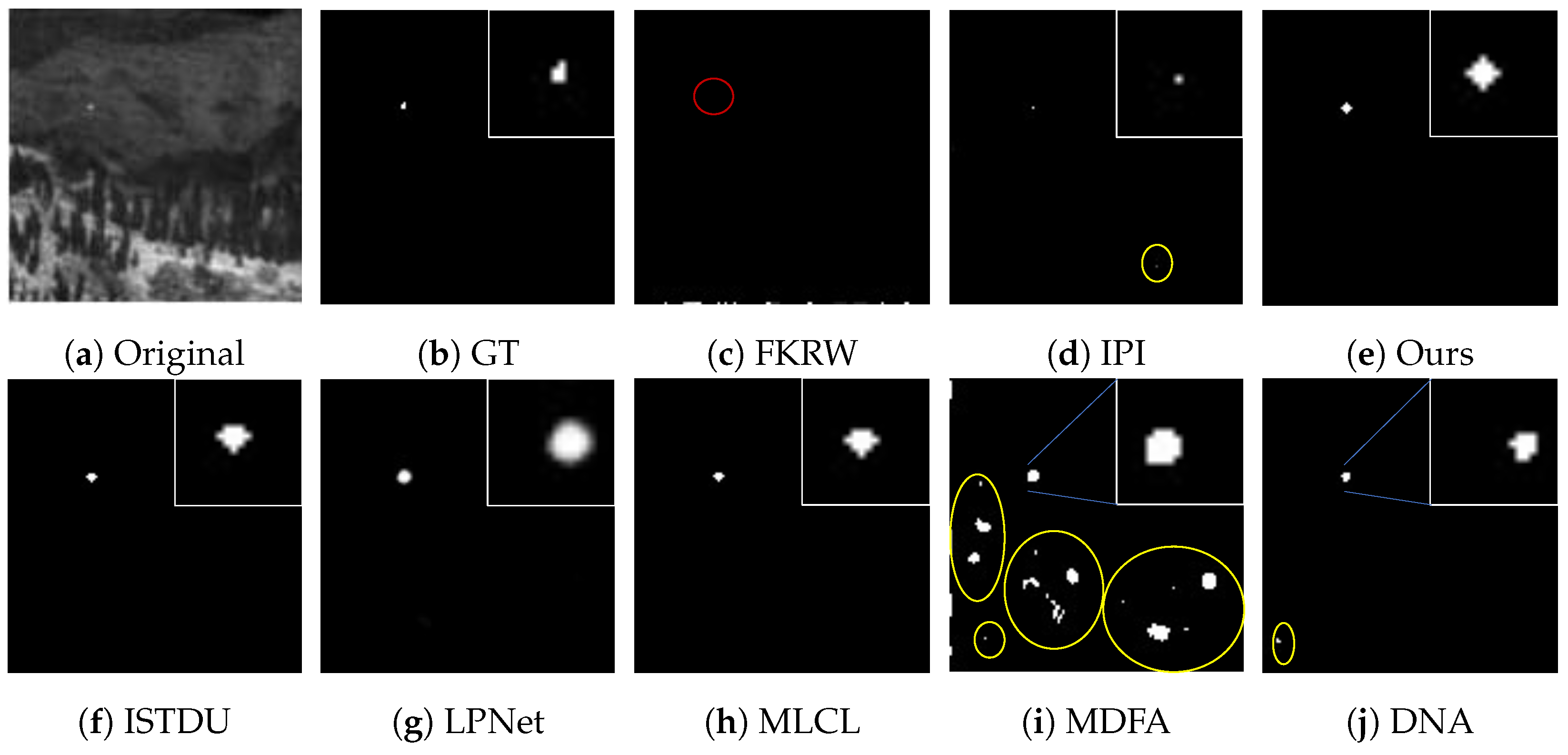
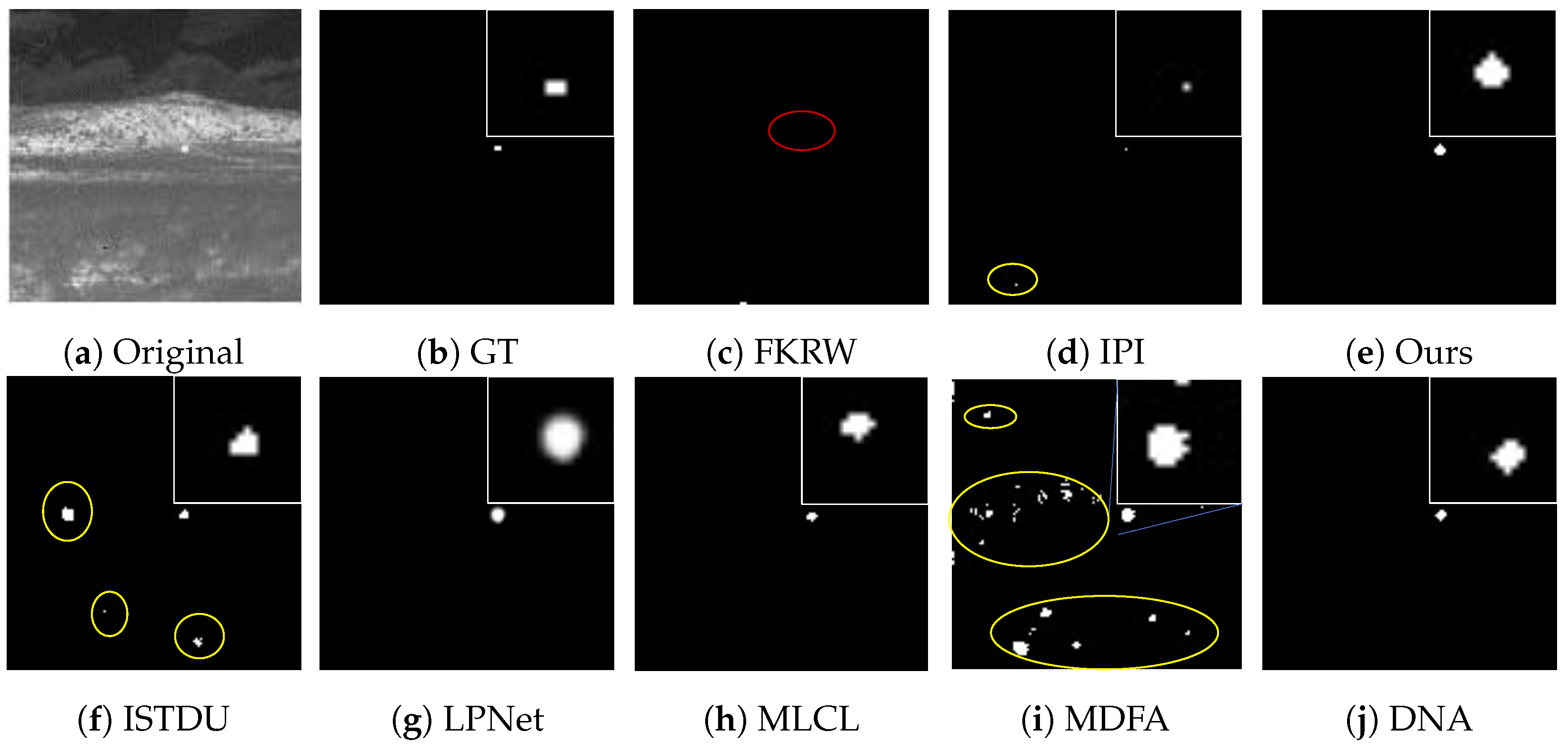
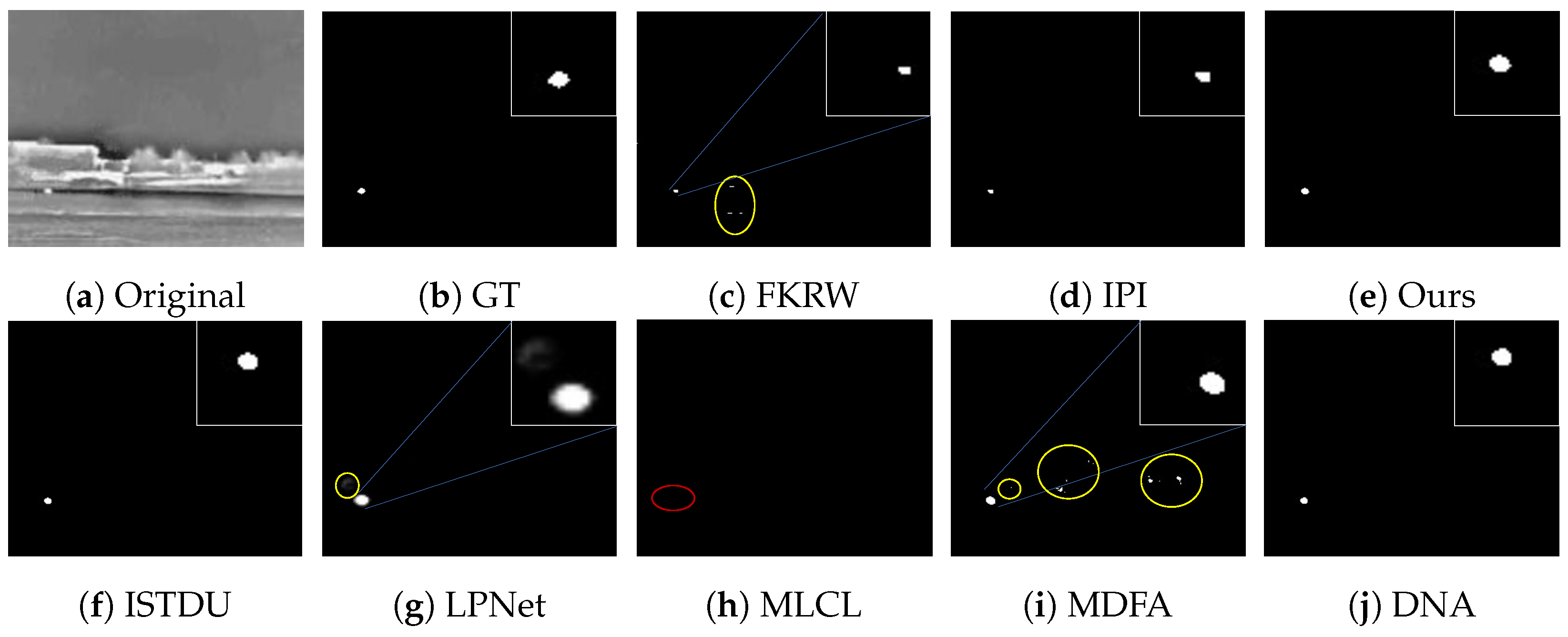
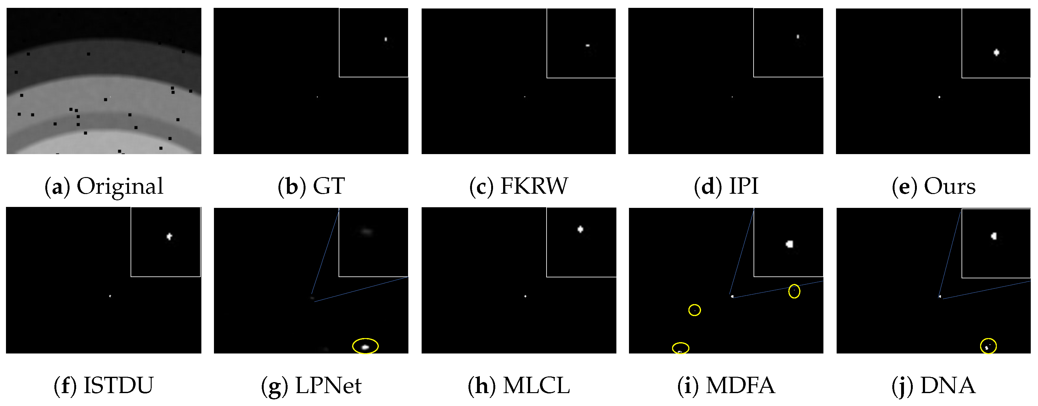
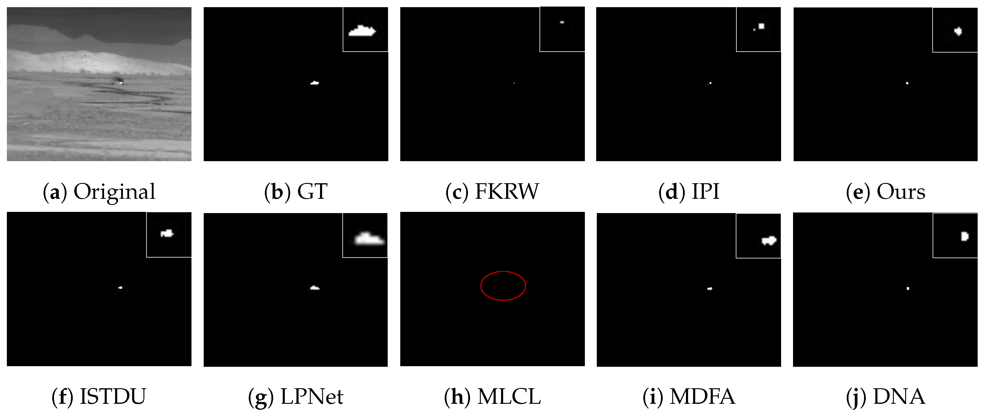
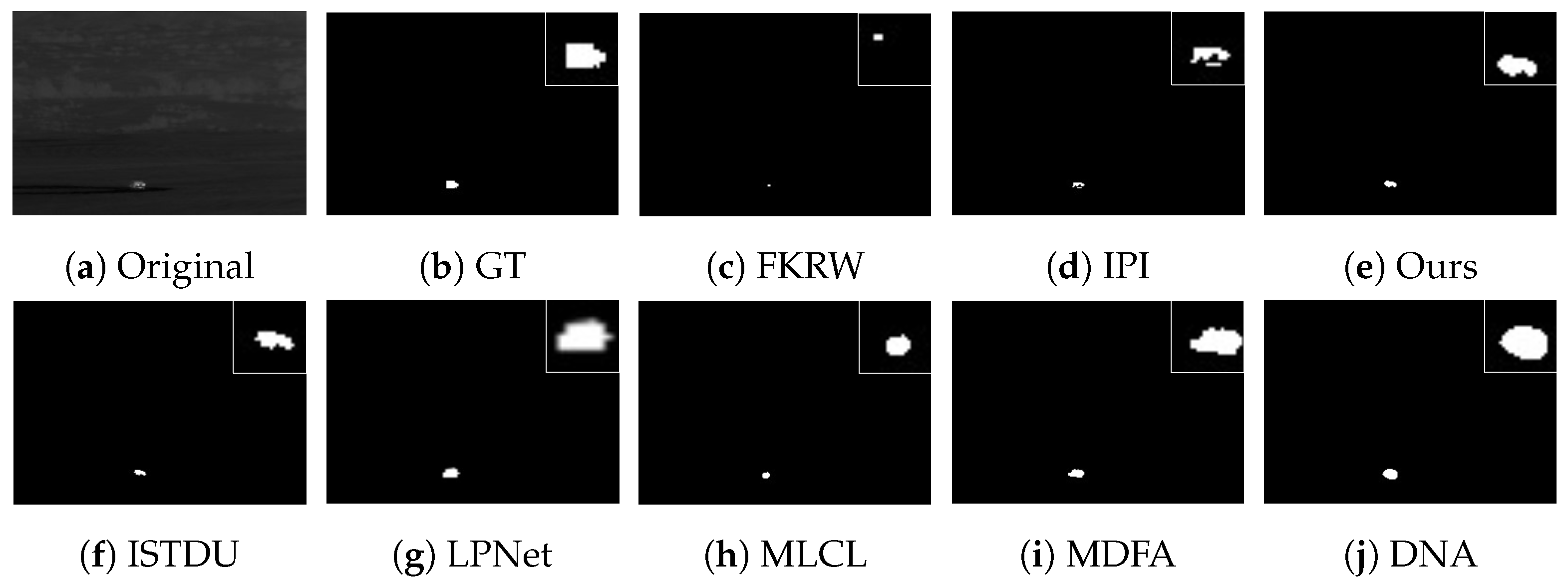
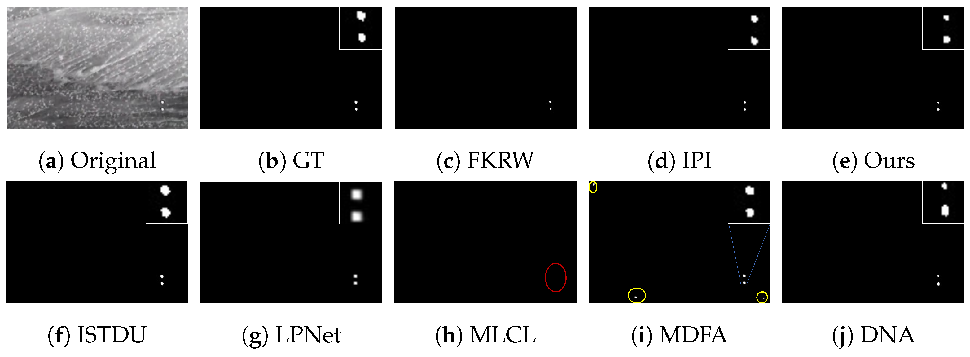
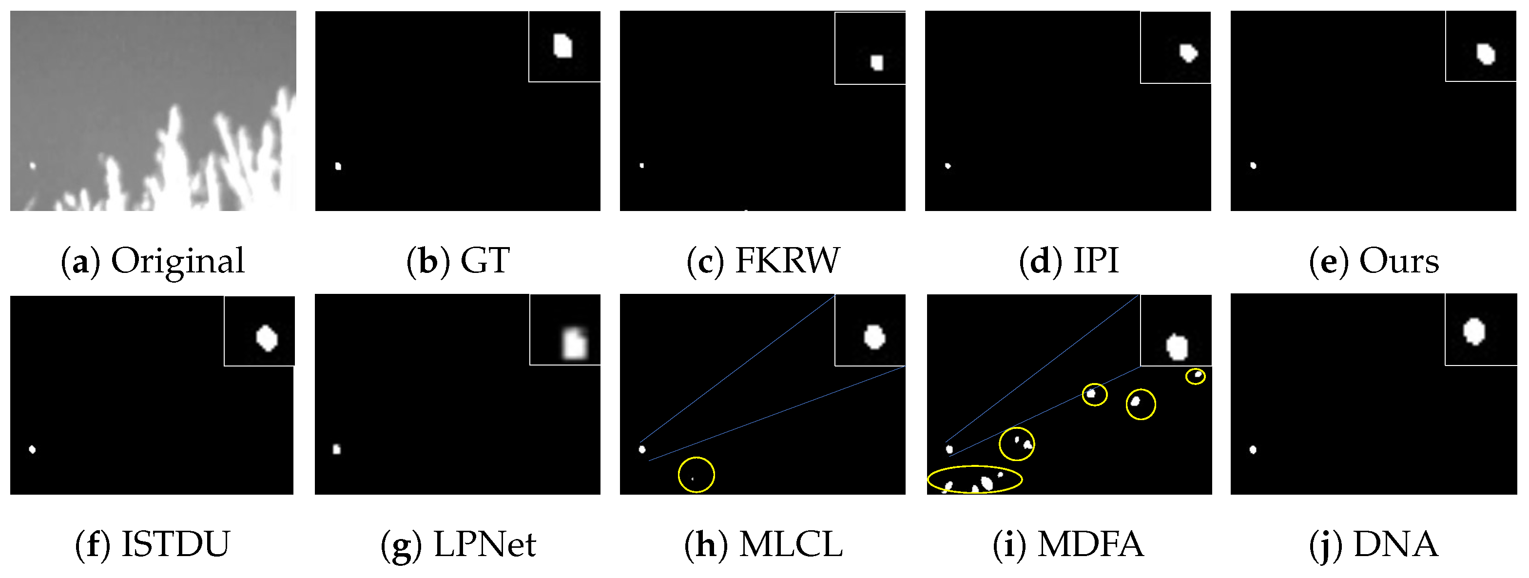
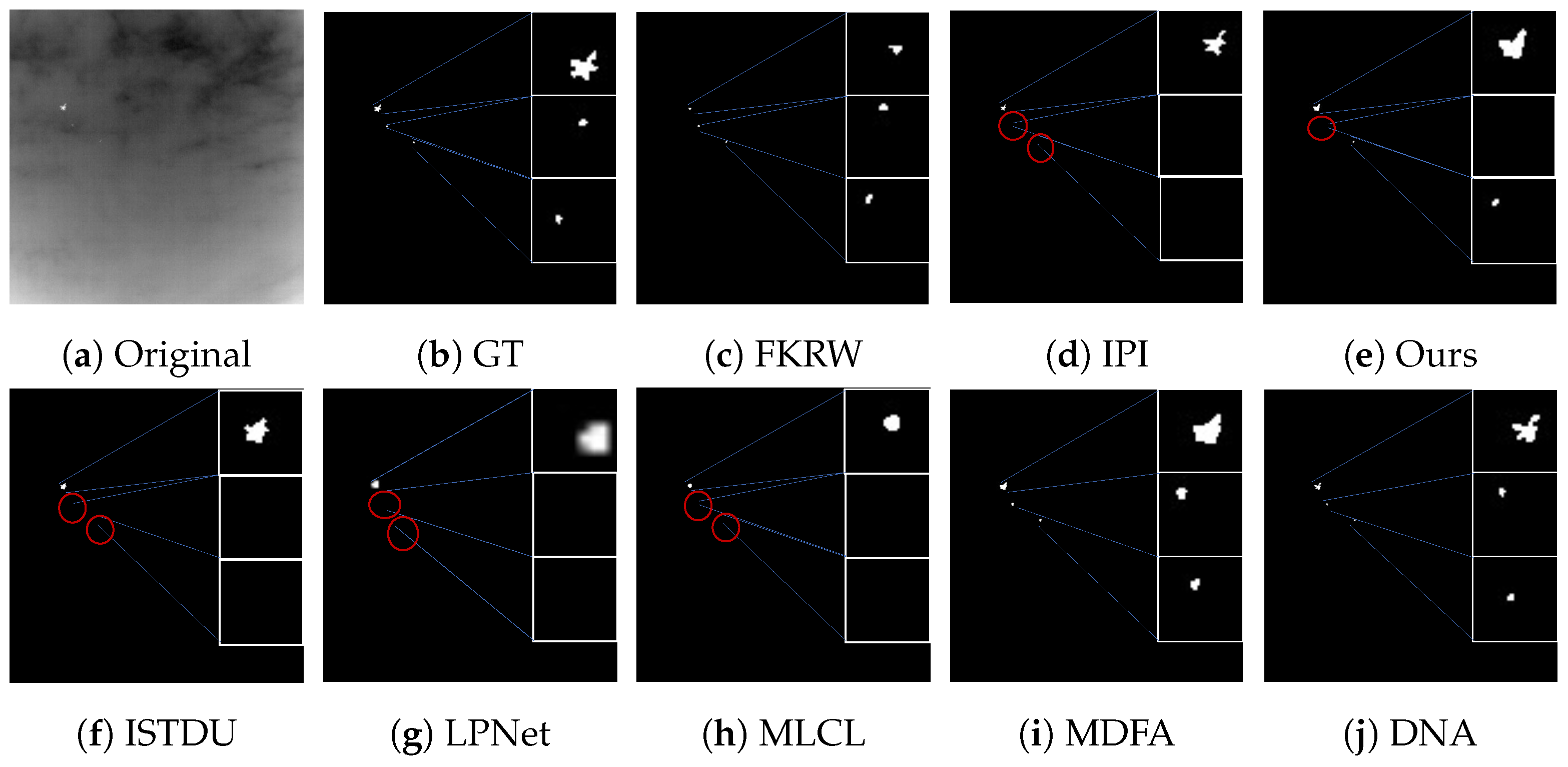
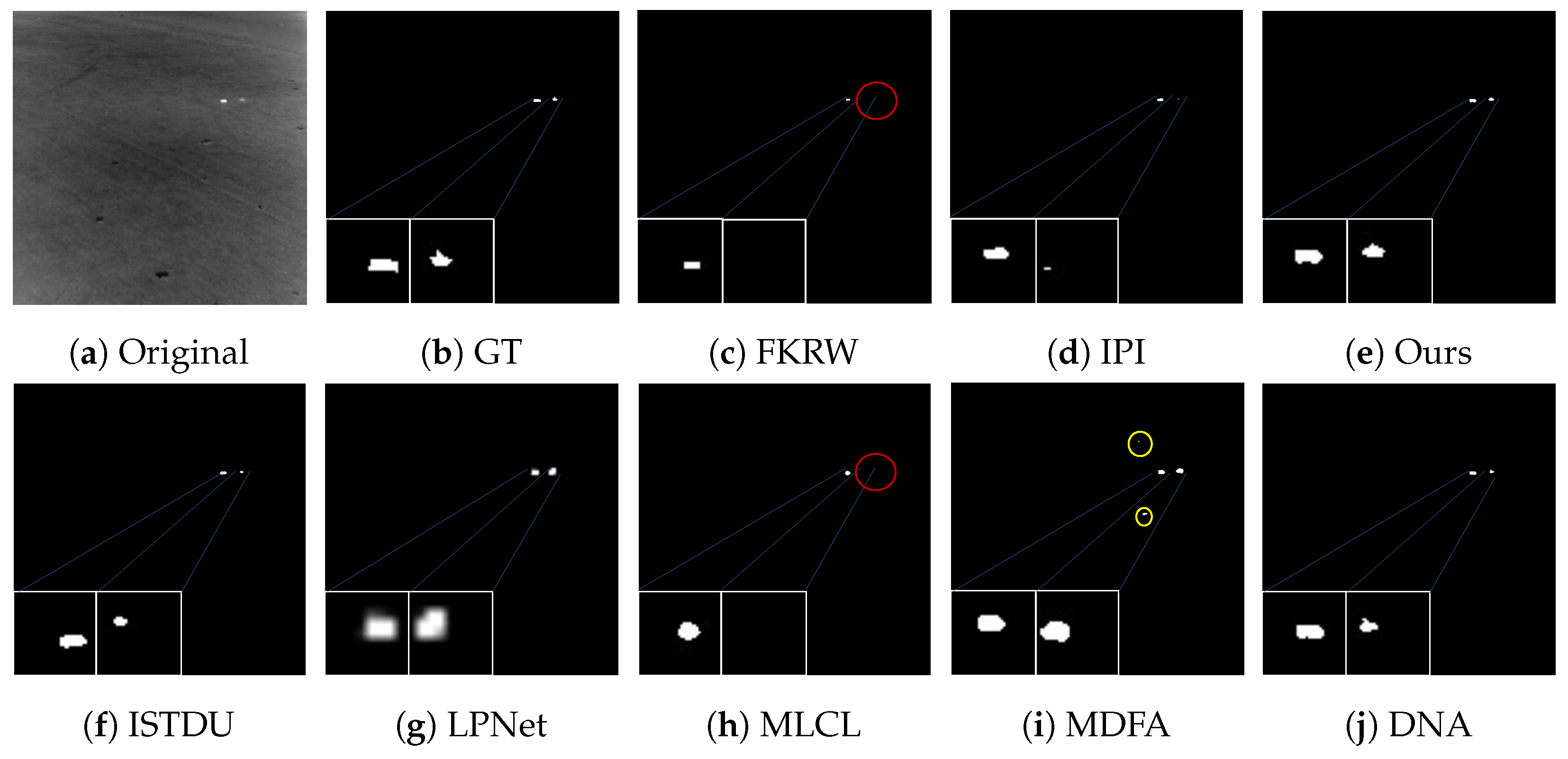
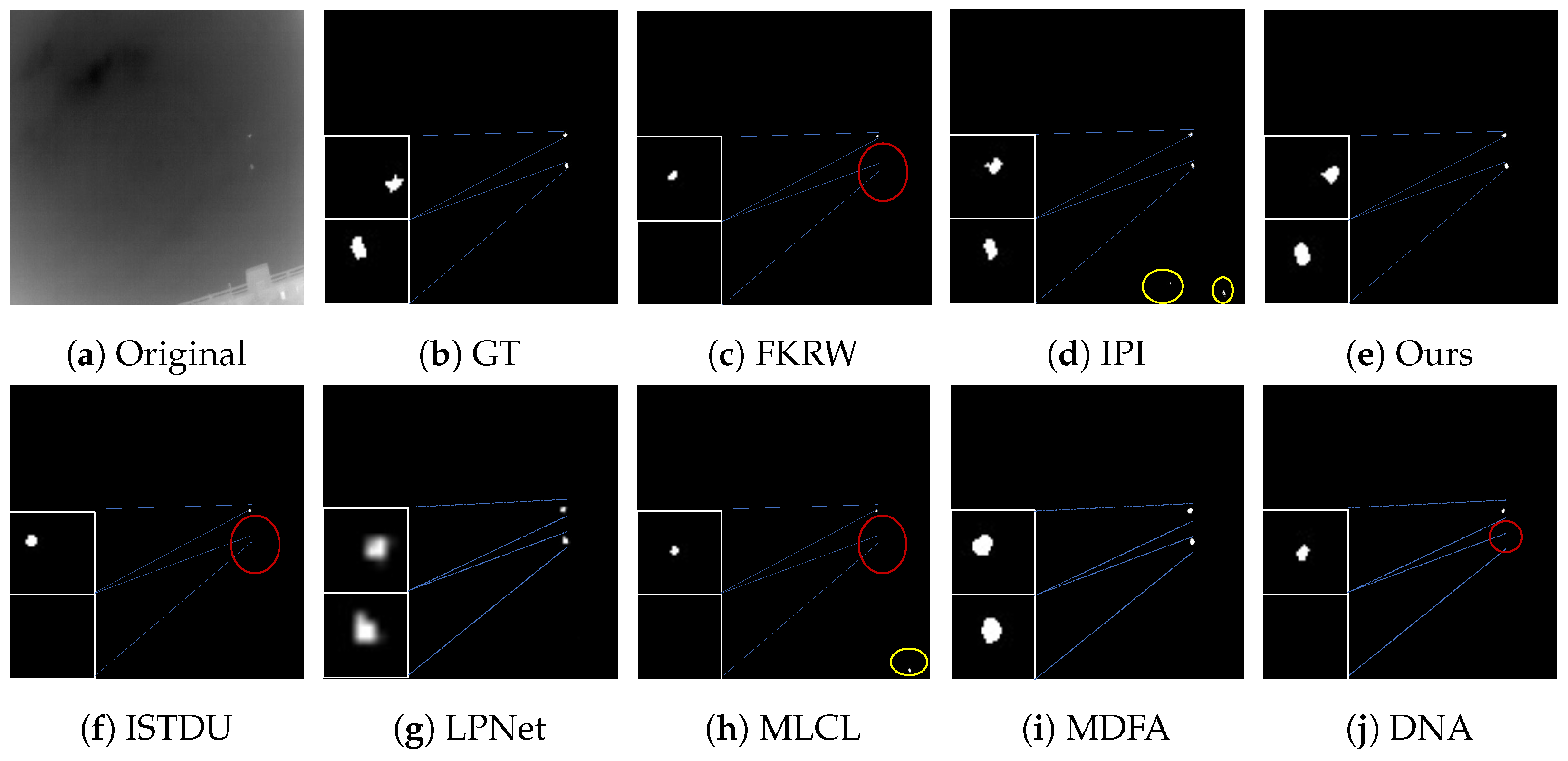
Some visualization examples of the MFIRST, SIRST, and IRSTD-1k datasets are shown in Figure 8, Figure 9, Figure 10, Figure 11, Figure 12, Figure 13, Figure 14, Figure 15, Figure 16, Figure 17, Figure 18 and Figure 19, respectively. The yellow circles in the images indicate false alarms, and the red circle indicates leakage detection. We zoomed in on the target, which is displayed in the white box in the corner of the images, and when there were multiple targets, a blue dotted line is used to show the correspondence between the target and its zoomed-in image.
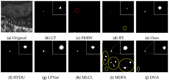
Figure 8.
Visual example one of some representative methods for the MFIRST dataset.
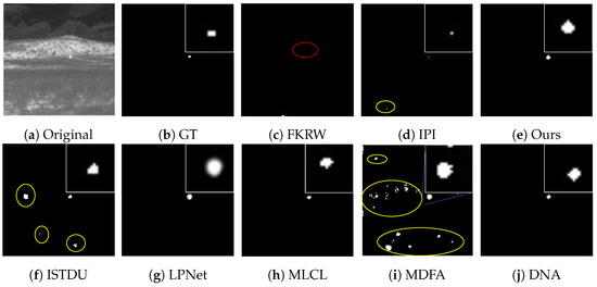
Figure 9.
Visual example two of some representative methods for the MFIRST dataset.
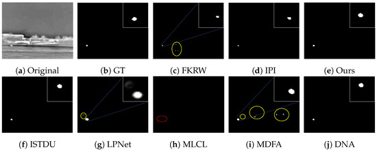
Figure 10.
Visual example three of some representative methods for the MFIRST dataset.
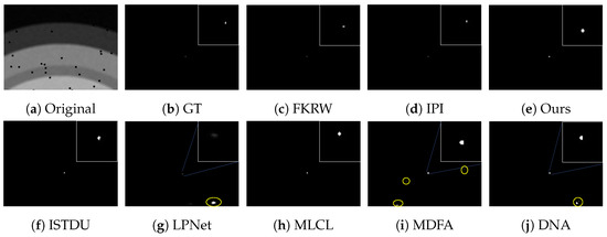
Figure 11.
Visual example four of some representative methods for the MFIRST dataset.

Figure 12.
Visual example one of some representative methods for the SIRST dataset.

Figure 13.
Visual example two of some representative methods for the SIRST dataset.
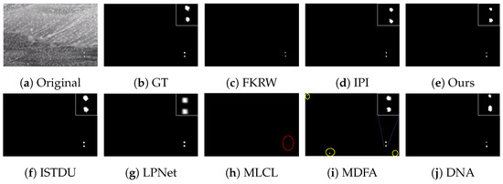
Figure 14.
Visual example three of some representative methods for the SIRST dataset.
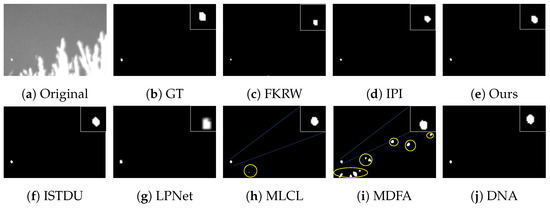
Figure 15.
Visual example four of some representative methods for the SIRST dataset.
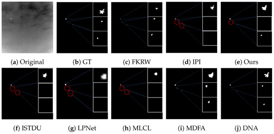
Figure 16.
Visual example one of some representative methods for the IRSTD-1k dataset.
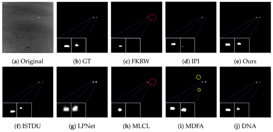
Figure 17.
Visual example two of some representative methods for the IRSTD-1k dataset.
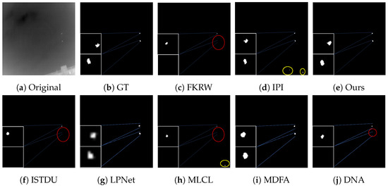
Figure 18.
Visual example three of some representative methods for the IRSTD-1k dataset.
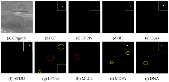
Figure 19.
Visual example four of some representative methods for the IRSTD-1k dataset.
Among the traditional algorithms, IPI had a high detection rate, but the false alarm rate was also higher; the FKRW algorithm resulted in some leakage detection, and noise was introduced at the bottom edge of the image; the MPCM algorithm was very sensitive to boundary changes, had the highest false alarm rate, and had difficulty discriminating between the target and false alarms, so the detection effect figure for MPCM is not included. Overall, the traditional algorithms did not exhibit as good detection performance as the deep learning algorithms due to their reliance on a priori knowledge and lack of generalization ability.
Among the deep learning algorithms, MLCL had fewer false alarms but more false alarms; MDFA has few false alarms but many false alarms, even worse than the traditional IPI algorithm; ISTDU and DNA could detect all the targets but had false alarms to different degrees; LPNet could accurately detect all targets, but the target became blurred and less information was retained following subsequent processing. Thanks to the ability of our MCSAM to better localize the target area and our algorithm’s advantages in extracting different features, our algorithm achieved the best detection results. Compared to other deep learning algorithms, our proposed algorithm could accurately detect all targets and achieved the lowest leakage and false alarm rates.
4. Discussion
Considering both the above quantitative and visual comparisons, the deep learning algorithms generally outperformed the traditional algorithms in terms of rates of detection and missed detection. Deep learning algorithms can extract rich feature information and automatically learn the features of a dataset through training, thus improving the detection efficacy of the algorithms, whereas traditional algorithms rely on a priori knowledge and can only be adapted to specific scenarios, making it difficult to detect targets in complex backgrounds.
Our algorithm can have different receptive fields through multiscale feature extraction, which improves its ability to adapt to targets of different sizes, including very small targets, and a high detection rate can be achieved. By using MCSAM, global information can be extracted and the target area can be made more prominent, thus improving detection in complex scenes and helping to achieve extremely low false alarm rates. In terms of quantitative metrics, our algorithm outperformed other state-of-the-art algorithms: we achieved the highest detection rate, the lowest false alarm rate, and the highest IoU values with different datasets; moreover, our ROC curve was closest to the upper left. Ablation and comparison experiments with different data demonstrate that our proposed amendments can effectively improve the detection performance of the algorithm.
5. Conclusions
In this paper, we present our proposed multiscale feature extraction U-Net network called MFEU-Net. MFEU-Net uses RSU and Inception as the encoder and decoder and extracts rich multiscale feature information through skip connections and a parallel branching structure, which enables the network to have different receptive field sizes at different layers. In addition, through MCSAM, weighting is performed in the channel and spatial domains separately, so the model can automatically learn the key patterns and features in the data, thereby focusing on the important regions in the feature map and thus improving its performance. In the experiments with different datasets, MFEU-Net achieved better detection results, demonstrating its effectiveness and that the changes result in an advancement.
Author Contributions
Conceptualization, X.W. (Xiaozhen Wang); methodology, X.W. (Xiaozhen Wang); software, X.W. (Xiaozhen Wang) and M.L.; validation, X.W. (Xiaofeng Wang), C.H.; writing—original draft preparation, X.W. (Xiaozhen Wang) and J.L.; writing—review and editing, X.W. (Xiaozhen Wang), T.N., M.L. and L.H. All authors have read and agreed to the published version of the manuscript.
Funding
This work was supported by the National Natural Science Foundation of China (No. 62105328).
Data Availability Statement
The SIRST, MFIRST, and IRSTD-1k image data used to support the research are available from the websites https://github.com/YimianDai/sirst, accessed on 29 July 2020, https://github.com/wanghuanphd/MDvsFAcGAN, accessed on 4 December 2019, https://github.com/RuiZhang97/ISNet, accessed on 20 March 2022.
Acknowledgments
The authors would like to thank D.Y., W.H. and Z.M. for providing the data.
Conflicts of Interest
The authors declare no conflicts of interest.
References
- Zhang, K.; Ni, S.; Yan, D.; Zhang, A. Review of dim small target detection algorithms in single-frame infrared images. In Proceedings of the 2021 IEEE 4th Advanced Information Management, Communicates, Electronic and Automation Control Conference (IMCEC), Chongqing, China, 18–20 June 2021; Volume 4, pp. 2115–2120. [Google Scholar]
- Wang, W.; Xiao, C.; Dou, H.; Liang, R.; Yuan, H.; Zhao, G.; Chen, Z.; Huang, Y. CCRANet: A Two-Stage Local Attention Network for Single-Frame Low-Resolution Infrared Small Target Detection. Remote Sens. 2023, 15, 5539. [Google Scholar] [CrossRef]
- Eysa, R.; Hamdulla, A. Issues on Infrared Dim Small Target Detection and Tracking. In Proceedings of the 2019 International Conference on Smart Grid and Electrical Automation (ICSGEA), Xiangtan, China, 10–11 August 2019; pp. 452–456. [Google Scholar] [CrossRef]
- Hao, X.; Liu, X.; Liu, Y.; Cui, Y.; Lei, T. Infrared Small-Target Detection Based on Background-Suppression Proximal Gradient and GPU Acceleration. Remote Sens. 2023, 15, 5424. [Google Scholar] [CrossRef]
- Rawat, S.S.; Verma, S.K.; Kumar, Y. Review on recent development in infrared small target detection algorithms. Procedia Comput. Sci. 2020, 167, 2496–2505. [Google Scholar] [CrossRef]
- Hou, Q.; Wang, Z.; Tan, F.; Zhao, Y.; Zheng, H.; Zhang, W. RISTDnet: Robust infrared small target detection network. IEEE Geosci. Remote Sens. Lett. 2021, 19, 7000805. [Google Scholar] [CrossRef]
- Wang, Y.; Cao, L.; Su, K.; Dai, D.; Li, N.; Wu, D. Infrared Moving Small Target Detection Based on Space–Time Combination in Complex Scenes. Remote Sens. 2023, 15, 5380. [Google Scholar] [CrossRef]
- Marvasti, F.S.; Mosavi, M.R.; Nasiri, M. Flying small target detection in IR images based on adaptive toggle operator. IET Comput. Vis. 2018, 12, 527–534. [Google Scholar] [CrossRef]
- Chen, Y.; Li, L.; Liu, X.; Su, X. A multi-task framework for infrared small target detection and segmentation. IEEE Trans. Geosci. Remote Sens. 2022, 60, 5003109. [Google Scholar] [CrossRef]
- Kim, S.; Song, W.J.; Kim, S.H. Double weight-based SAR and infrared sensor fusion for automatic ground target recognition with deep learning. Remote Sens. 2018, 10, 72. [Google Scholar] [CrossRef]
- Kwan, C.; Chou, B.; Yang, J.; Tran, T. Deep learning based target tracking and classification for infrared videos using compressive measurements. J. Signal Inf. Process. 2019, 10, 167. [Google Scholar] [CrossRef][Green Version]
- Ju, M.; Luo, J.; Liu, G.; Luo, H. ISTDet: An efficient end-to-end neural network for infrared small target detection. Infrared Phys. Technol. 2021, 114, 103659. [Google Scholar] [CrossRef]
- Yao, J.; Xiao, S.; Deng, Q.; Wen, G.; Tao, H.; Du, J. An Infrared Maritime Small Target Detection Algorithm Based on Semantic, Detail, and Edge Multidimensional Information Fusion. Remote Sens. 2023, 15, 4909. [Google Scholar] [CrossRef]
- Kim, J.H.; Hwang, Y. GAN-based synthetic data augmentation for infrared small target detection. IEEE Trans. Geosci. Remote Sens. 2022, 60, 5002512. [Google Scholar] [CrossRef]
- Zhang, M.; Yang, H.; Yue, K.; Zhang, X.; Zhu, Y.; Li, Y. Thermodynamics-Inspired Multi-Feature Network for Infrared Small Target Detection. Remote Sens. 2023, 15, 4716. [Google Scholar] [CrossRef]
- Zuo, Z.; Tong, X.; Wei, J.; Su, S.; Wu, P.; Guo, R.; Sun, B. AFFPN: Attention fusion feature pyramid network for small infrared target detection. Remote Sens. 2022, 14, 3412. [Google Scholar] [CrossRef]
- Deshpande, S.D.; Er, M.H.; Venkateswarlu, R.; Chan, P. Max-mean and max-median filters for detection of small targets. In Proceedings of the Signal and Data Processing of Small Targets 1999, Denver, CO, USA, 4 October 1999; Volume 3809, pp. 74–83. [Google Scholar]
- Starck, J.L.; Candès, E.J.; Donoho, D.L. The curvelet transform for image denoising. IEEE Trans. Image Process. 2002, 11, 670–684. [Google Scholar] [CrossRef] [PubMed]
- Chen, C.P.; Li, H.; Wei, Y.; Xia, T.; Tang, Y.Y. A local contrast method for small infrared target detection. IEEE Trans. Geosci. Remote Sens. 2013, 52, 574–581. [Google Scholar] [CrossRef]
- Han, J.; Moradi, S.; Faramarzi, I.; Liu, C.; Zhang, H.; Zhao, Q. A local contrast method for infrared small-target detection utilizing a tri-layer window. IEEE Geosci. Remote Sens. Lett. 2019, 17, 1822–1826. [Google Scholar] [CrossRef]
- Wei, Y.; You, X.; Li, H. Multiscale patch-based contrast measure for small infrared target detection. Pattern Recognit. 2016, 58, 216–226. [Google Scholar] [CrossRef]
- Sun, Y.; Yang, J.; An, W. Infrared dim and small target detection via multiple subspace learning and spatial-temporal patch-tensor model. IEEE Trans. Geosci. Remote Sens. 2020, 59, 3737–3752. [Google Scholar] [CrossRef]
- Zhang, L.; Peng, L.; Zhang, T.; Cao, S.; Peng, Z. Infrared small target detection via non-convex rank approximation minimization joint l 2, 1 norm. Remote Sens. 2018, 10, 1821. [Google Scholar] [CrossRef]
- Baili, N.; Moalla, M.; Frigui, H.; Karem, A.D. Multistage approach for automatic target detection and recognition in infrared imagery using deep learning. J. Appl. Remote Sens. 2022, 16, 048505. [Google Scholar] [CrossRef]
- Wang, H.; Zhou, L.; Wang, L. Miss detection vs. false alarm: Adversarial learning for small object segmentation in infrared images. In Proceedings of the IEEE/CVF International Conference on Computer Vision, Seoul, Republic of Korea, 27 October–2 November 2019; pp. 8509–8518. [Google Scholar]
- Li, B.; Xiao, C.; Wang, L.; Wang, Y.; Lin, Z.; Li, M.; An, W.; Guo, Y. Dense nested attention network for infrared small target detection. IEEE Trans. Image Process. 2022, 32, 1745–1758. [Google Scholar] [CrossRef] [PubMed]
- Chen, F.; Gao, C.; Liu, F.; Zhao, Y.; Zhou, Y.; Meng, D.; Zuo, W. Local patch network with global attention for infrared small target detection. IEEE Trans. Aerosp. Electron. Syst. 2022, 58, 3979–3991. [Google Scholar] [CrossRef]
- Hou, Q.; Zhang, L.; Tan, F.; Xi, Y.; Zheng, H.; Li, N. ISTDU-Net: Infrared Small-Target Detection U-Net. IEEE Geosci. Remote Sens. Lett. 2022, 19, 7506205. [Google Scholar] [CrossRef]
- Yu, C.; Liu, Y.; Wu, S.; Hu, Z.; Xia, X.; Lan, D.; Liu, X. Infrared small target detection based on multiscale local contrast learning networks. Infrared Phys. Technol. 2022, 123, 104107. [Google Scholar] [CrossRef]
- Li, R.; Shen, Y. YOLOSR-IST: A deep learning method for small target detection in infrared remote sensing images based on super-resolution and YOLO. Signal Process. 2023, 208, 108962. [Google Scholar] [CrossRef]
- Zhang, M.; Zhang, R.; Zhang, J.; Guo, J.; Li, Y.; Gao, X. Dim2Clear network for infrared small target detection. IEEE Trans. Geosci. Remote Sens. 2023, 61, 5001714. [Google Scholar] [CrossRef]
- Hu, J.; Shen, L.; Sun, G. Squeeze-and-excitation networks. In Proceedings of the IEEE Conference on Computer Vision and Pattern Recognition, Salt Lake City, UT, USA, 18–23 June 2018; pp. 7132–7141. [Google Scholar]
- Wang, Q.; Wu, B.; Zhu, P.; Li, P.; Zuo, W.; Hu, Q. ECA-Net: Efficient channel attention for deep convolutional neural networks. In Proceedings of the IEEE/CVF Conference on Computer Vision and Pattern Recognition, Seattle, WA, USA, 13–19 June 2020; pp. 11534–11542. [Google Scholar]
- Woo, S.; Park, J.; Lee, J.Y.; Kweon, I.S. Cbam: Convolutional block attention module. In Proceedings of the European Conference on Computer Vision (ECCV), Munich, Germany, 8–14 September 2018; pp. 3–19. [Google Scholar]
- Qin, X.; Zhang, Z.; Huang, C.; Dehghan, M.; Zaiane, O.R.; Jagersand, M. U2-Net: Going deeper with nested U-structure for salient object detection. Pattern Recognit. 2020, 106, 107404. [Google Scholar] [CrossRef]
- Szegedy, C.; Ioffe, S.; Vanhoucke, V.; Alemi, A. Inception-ResNet and the impact of residual connections on learning. arXiv 2016, arXiv:1602.07261. [Google Scholar]
- Li, X.; Sun, X.; Meng, Y.; Liang, J.; Wu, F.; Li, J. Dice loss for data-imbalanced NLP tasks. arXiv 2019, arXiv:1911.02855. [Google Scholar]
- Lin, T.Y.; Goyal, P.; Girshick, R.; He, K.; Dollár, P. Focal loss for dense object detection. In Proceedings of the IEEE International Conference on Computer Vision, Venice, Italy, 22–29 October 2017; pp. 2980–2988. [Google Scholar]
- Cheng, B.; Girshick, R.; Dollár, P.; Berg, A.C.; Kirillov, A. Boundary IoU: Improving object-centric image segmentation evaluation. In Proceedings of the IEEE/CVF Conference on Computer Vision and Pattern Recognition, Nashville, TN, USA, 20–25 June 2021; pp. 15334–15342. [Google Scholar]
- Dai, Y.; Wu, Y.; Zhou, F.; Barnard, K. Asymmetric contextual modulation for infrared small target detection. In Proceedings of the IEEE/CVF Winter Conference on Applications of Computer Vision, Waikoloa, HI, USA, 3–8 January 2021; pp. 950–959. [Google Scholar]
- Zhang, M.; Zhang, R.; Yang, Y.; Bai, H.; Zhang, J.; Guo, J. ISNet: Shape Matters for Infrared Small Target Detection. In Proceedings of the 2022 IEEE/CVF Conference on Computer Vision and Pattern Recognition (CVPR), New Orleans, LA, USA, 18–24 June 2022; pp. 867–876. [Google Scholar] [CrossRef]
- Gao, C.; Meng, D.; Yang, Y.; Wang, Y.; Zhou, X.; Hauptmann, A.G. Infrared patch-image model for small target detection in a single image. IEEE Trans. Image Process. 2013, 22, 4996–5009. [Google Scholar] [CrossRef] [PubMed]
- Qin, Y.; Bruzzone, L.; Gao, C.; Li, B. Infrared small target detection based on facet kernel and random walker. IEEE Trans. Geosci. Remote Sens. 2019, 57, 7104–7118. [Google Scholar] [CrossRef]
Disclaimer/Publisher’s Note: The statements, opinions and data contained in all publications are solely those of the individual author(s) and contributor(s) and not of MDPI and/or the editor(s). MDPI and/or the editor(s) disclaim responsibility for any injury to people or property resulting from any ideas, methods, instructions or products referred to in the content. |
© 2024 by the authors. Licensee MDPI, Basel, Switzerland. This article is an open access article distributed under the terms and conditions of the Creative Commons Attribution (CC BY) license (https://creativecommons.org/licenses/by/4.0/).

