Abstract
Remote sensing (RS) technology can rapidly obtain spatial distribution information on soil salinization. However, (1) the scale effects resulting from the mismatch between ground-based “point” salinity data and remote sensing pixel-based “spatial” data often limit the accuracy of remote sensing monitoring of soil salinity, and (2) the same salinity RS monitoring model usually provides inconsistent or sometimes conflicting explanations for different data. Therefore, based on Landsat 8 imagery and synchronously collected ground-sampling data of two typical study regions (denoted as N and S, respectively) of the Yichang Irrigation Area in the Hetao Irrigation District for May 2013, this study used geostatistical methods to obtain “relative truth values” of salinity corresponding to the Landsat 8 pixel scale. Additionally, based on Landsat 8 multispectral data, 14 salinity indices were constructed. Subsequently, the Correlation-based Feature Selection (CFS) method was used to select sensitive features, and a strategy similar to the concept of ensemble learning (EL) was adopted to integrate the single-feature-sensitive Bayesian classification (BC) model in order to construct an RS monitoring model for soil salinization (Nonsaline, Slightly saline, Moderately saline, Strongly saline, and Solonchak). The research results indicated that (1) soil salinity exhibits moderate to strong variability within a 30 m scale, and the spatial heterogeneity of soil salinity needs to be considered when developing remote sensing models; (2) the theoretical models of salinity variance functions in the N and S regions conform to the exponential model and the spherical model, with values of 0.817 and 0.967, respectively, indicating a good fit for the variance characteristics of salinity and suitability for Kriging interpolation; and (3) compared to a single-feature BC model, the soil salinization identification model constructed using the concept of EL demonstrated better potential for robustness and effectiveness.
1. Introduction
Soil salinization is a global issue of concern to resources and ecology [1,2]. It usually results from the interaction of natural or anthropogenic factors such as climate, topography, hydrogeology, and irrigated agriculture, particularly in arid or semi-arid regions [3,4,5]. Soil salinization can lead to changes in soil properties, resulting in a decrease in soil potential productivity and posing a serious threat to resources and the environment. It is widely recognized as one of the main factors to consider in achieving sustainable agriculture and land management [6]. Therefore, the timely and accurate assessment of the degree and distribution of soil salinization in salt-affected areas is of great significance for comprehensively formulating scientific management measures and the rational utilization of land resources.
Remote sensing (RS) technology provides a fast and reliable approach for the timely and accurate acquisition of information on salt-affected soils, enabling the dynamic monitoring of regional soil salinization [1]. In soil salinization RS monitoring, ground point observation data are commonly used to calibrate RS information and verify inversion results [7,8,9]. However, due to the strong spatiotemporal heterogeneity of soil salinity [10,11], even ground point observations taken at the same time cannot fully represent the corresponding observations at the pixel scale of RS. Geostatistical methods (e.g., variograms and Kriging interpolation) are efficient for obtaining soil property information from surface data, and the obtained “RS spatial data” are more representative than information obtained from individual sampling points. However, most studies focus on the analysis of spatial heterogeneity and scale effects of ground point observation data [12,13] and rarely combine this information with RS data to better monitor soil salinization.
Over the years, the effective detection of salt-affected soils using RS has mainly relied on the spectral response characteristics of saline soils [14]. Generally, reflectance increases with an increasing quantity of salts at the terrain surface [1], providing an important scientific basis for RS monitoring of soil salinization. However, RS images are susceptible to the “same spectrum for different objects, different spectra for the same object” phenomenon due to atmospheric conditions, sensor characteristics, and other factors. This makes the correspondence between the degree of soil salinization and spectral response characteristics not always clear, making it difficult for rule-based classification methods (such as decision trees, random forests, etc.) to solve this problem effectively. Compared to rule-based classification methods, Bayesian methods are non-rule-based classification methods that achieve optimal statistical classification results based on class priors and class probability density functions. In recent years, theoretical and applied research on Bayesian statistics both nationally and in other countries has increased, and their application in research on extreme climate risk [15,16,17], sediment fingerprinting identification [18,19,20], soil properties [21,22], and many other fields has become widespread and demonstrated significant application potential.
Although Bayesian methods are ideal for soil salinity modeling, as with any other method, models may have similar performance using different input variables but offering different predictions [23,24]. Ensemble learning (EL) is a machine learning framework based on the idea of “group intelligence”, which is capable of combining (averaging) the predictions of multiple participating models [25,26,27,28]. Compared to single-model predictions, EL can consistently generate more accurate and reliable predictions [29,30,31]. In practical applications, EL can be homogenous and heterogeneous based on whether the participating models are of the same type [32]. In recent years, EL methods have been widely applied in soil modeling and analysis, such as in determining soil classes [33], soil properties [34,35,36], soil micronutrients [37], soil organic carbon [38,39], soil moisture [40,41], and soil texture [42,43]. However, the application of EL in soil salinization analysis is relatively limited. Therefore, it is of great research significance to effectively apply the advanced concept and method of EL to soil salinity monitoring research based on the comparison and evaluation of existing methods and models.
Therefore, this study conducted an “RS-ground synchronization experiment” in the Hetao Irrigation District, Inner Mongolia, aiming to (1) achieve the conversion of ground point data and RS pixel-scale salinity “relative truth values” and (2) evaluate the potential of the EL concept in predicting remote sensing monitoring of soil salinization.
2. Materials and Methods
2.1. Study Area
The study was conducted in the Hetao Irrigation District of Inner Mongolia in northwestern China, which is one of the three largest irrigation districts in China and the largest in Asia. The district is located at 40°10′–41°20′N, 106°10′–109°30′E, in the Hetao Plain of the Yellow River, with a flat topography, higher in the southwest and lower in the northeast. The elevation ranges from approximately 1007 m to 1050 m (with an average elevation of 1028 m). The annual average temperature ranges from 6.5 to 7.8 °C, with low rainfall and intense evaporation. The annual average precipitation ranges from 100 to 250 mm, while the evaporation can reach as high as 2400 mm, representing a typical temperate continental climate. The study area is an important production base for commodity grains and oil in the country and in the autonomous region, with major crops including wheat, coarse grains, maize, sugar beet, and sunflower, among others.
2.2. Data Acquisition and Processing
The research data mainly include two types of data: (1) soil salinity data and (2) satellite imagery data.
2.2.1. Salt Data Collection and Processing
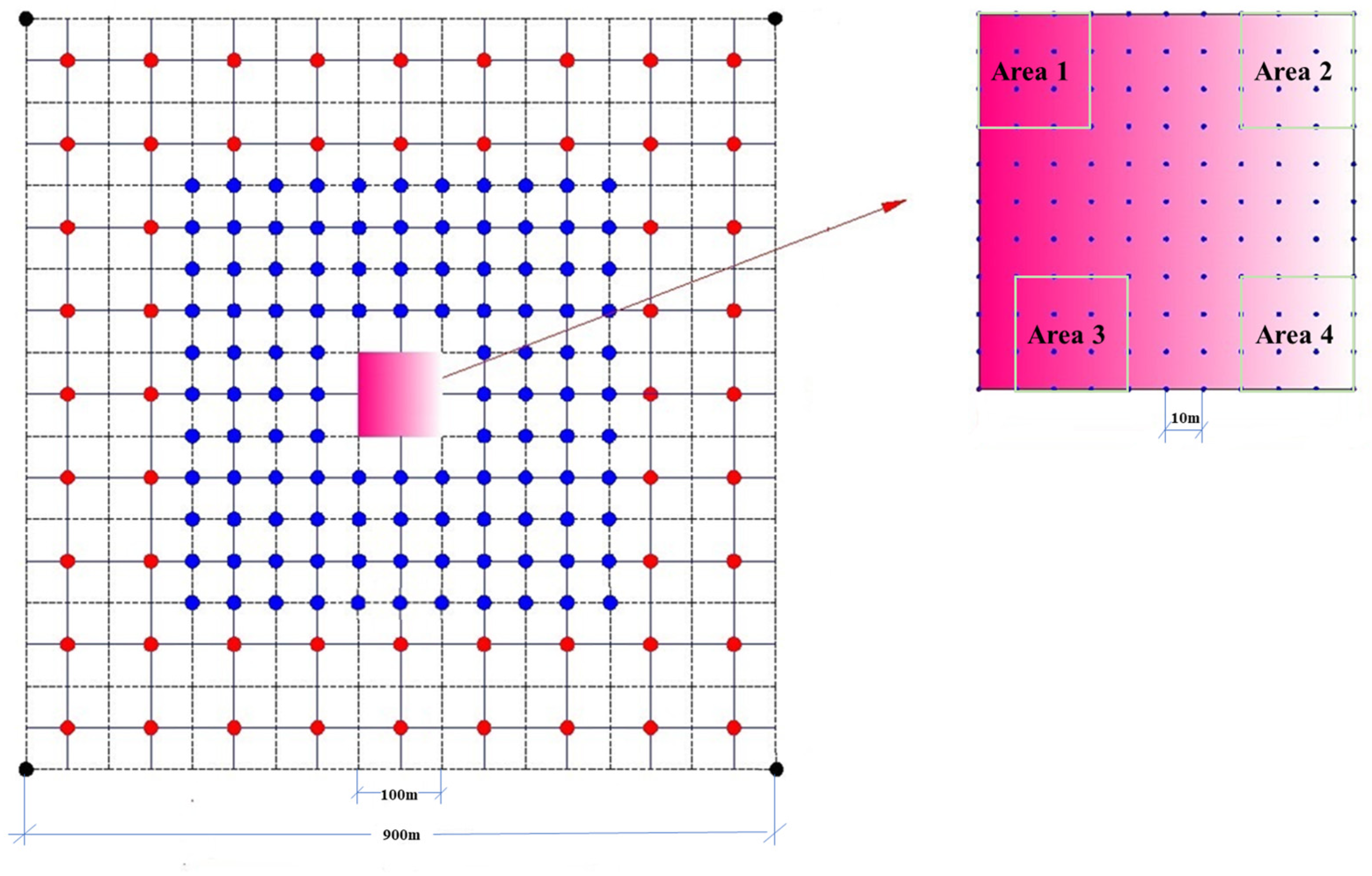
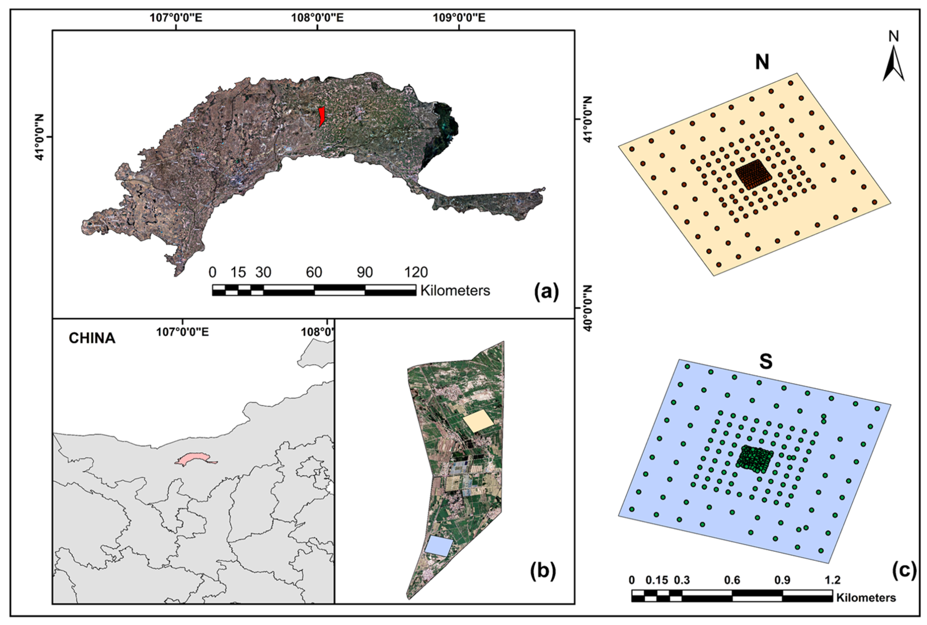
In the Yichang irrigation area of the Hetao Irrigation District, a research area of 2667 ha was selected. Two experimental regions (referred to as N and S regions) with an area of 64 ha each were selected within this research area, and the same sampling scheme was adopted for these two regions. The N area primarily consists of farmland, while the S region includes both farmland and regions affected by salinization. The sampling scheme is shown in Figure 1. Field surveys and soil sample collection were conducted in May 2013. A total of 243 soil samples were collected in the N research region, and 245 soil samples were collected in the S research region, resulting in a total of 488 surface (0–5 cm) soil samples. The collected soil samples were placed in sampling bags for subsequent laboratory analysis of soil salinity. To accurately record the coordinates of the sampling points, a GPS locator was used, as shown in Figure 2.
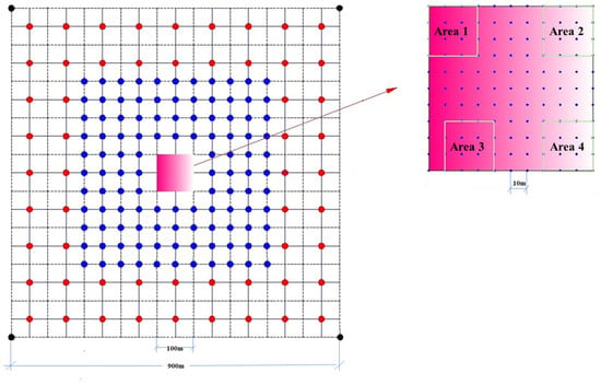
Figure 1.
Soil sampling scheme.
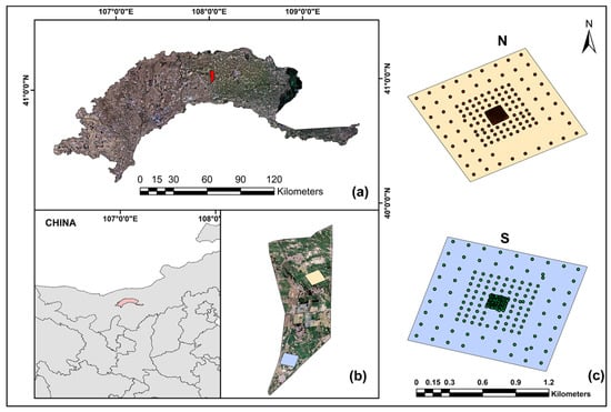
Figure 2.
Study area and sampling point map. (a) Hetao Irrigation District; (b) 2667 ha experimental area; (c) N and S experimental regions.
The collected soil samples were dried, sieved, grind, and passed through a 2 mm sieve in the laboratory. The electrical conductivity of the soil extract (EC1:5, dS/m) was determined using a conductivity meter at a soil-to-water ratio of 1:5. The soil salinity content (SSC, %) was calculated as , .
2.2.2. Landsat 8 Data Acquisition and Processing
Accounting for factors such as the actual conditions of the study area, the spatial resolution of the RS images, and the ease of image acquisition, the Landsat series of satellites from the United States was selected as the target RS data source. The spatial resolution of the images was 30 m. To ensure the accuracy of the data, Landsat 8 images (20 April 2013) that were close in time to ground sampling were obtained from the United States Geological Survey (USGS) platform (https://earthexplorer.usgs.gov/).
ENVI 5.3 software was used to perform preprocessing tasks of the Landsat 8 images, such as radiometric calibration, atmospheric correction, image stitching, and cropping.
2.2.3. Remote Sensing Pixel-Scale Salt Content Acquisition
To address the scale effects resulting from the mismatch between ground-based “point” salinity data and remote sensing pixel-based “spatial” data, a geostatistical approach was adopted, using the intended remote sensing image pixel scale as the interpolation scale to convert ground “point”-scale soil salt observations to pixel-scale soil salt content. Geostatistics consist of two main components: the analysis of spatial variation and structure using variograms and their parameters and the Kriging interpolation method for spatial-localization estimation.
- (1)
- Normality test of the data
The calculation of the variance function typically requires data to follow a normal distribution, as otherwise scale effects may occur. To assess whether the data followed a normal distribution, the Kolmogorov–Smirnov (K-S) test in SPSS 26 was used. If the data do not conform to a normal distribution, data transformation is applied to make it follow a normal distribution.
- (2)
- Variance function
The variance function is used to describe the structural and stochastic characteristics of regionalized variables. Its empirical function expression is
where represents the average variance of all point pairs spaced h apart; and represent the values of the study variable (such as observed values of a certain attribute or factor) at points and , respectively; and represents the numerical pairs with a spacing of h.
Theoretical models of the variance function are commonly used as exponential, spherical, Gaussian, and linear models. The structural characteristics of the variance function are described by four important parameters: the type of function, nugget variance (denoted as ), sill (denoted as , where represents the partial sill), and range (denoted as ). The GS + 9.0 software is used to compute the variance function, and the optimal theoretical model of the variance function is selected based on the principles of a high approaching 1 and the minimum residual sum of squares (RSS).
The spatial variation in soil salinity is influenced by two main factors: (1) random factors (related to irrigation, fertilization, cultivation practices, land-use practices, etc., i.e., human-associated factors) and (2) structural factors denoted as (related to topography, climate, vegetation, soil types, etc., i.e., natural factors). represents spatial correlation, indicating the proportion of spatial heterogeneity caused by random factors to the total variability of the system. If , there is a strong spatial correlation, and the spatial variation is mainly controlled by structural factors. If , there is a moderate spatial correlation, where spatial variation is influenced by both structural and random factors. If 75%, there is a weak spatial correlation, and the spatial variation is mainly governed by random factors.
- (3)
- Kriging interpolation
Kriging interpolation is an unbiased optimal estimation method based on the analysis of the distribution of the data of geographic variables and the structure of their variance functions, which is used to estimate the attribute values of unknown points [22,44]. During the interpolation process, Kriging considers the spatial relationship between the unknown points and all known sample points, fully utilizes the spatial structural characteristics of the sample point data, assigns a certain interpolation weight to each known point, and predicts the value of unknown points using a weighted average method.
In this study, the soil salinity was subjected to ordinary Kriging interpolation using the Spatial Analyst tool in ArcGIS 10.5 software. This allowed for the generation of soil salt content estimates corresponding to the Landat 8 (30 m × 30 m) pixel scale.
2.2.4. Classification Criteria for Soil Salinization
According to the soil salinization classification criteria used by Wu et al. [45], soil salinity can be divided into the following five levels: (a) Nonsaline: salt content < 0.2%; (b) Slightly saline: salt content ranging from 0.2% to 0.3%; (c) Moderately saline: salt content ranging from 0.3% to 0.6%; (d) Strongly saline: salt content ranging from 0.6% to 1.0%; and (e) Solonchak: salt content > 1.0%.
2.3. Spectral Index Construction
Spectral indices are commonly used as indirect indicators for monitoring salinized areas in bare ground or soils with very low vegetation cover. Spectral indices are obtained by combining two or more spectral bands and are widely regarded as powerful tools for identifying features of interest [8]. Based on existing research and experience, 14 commonly used salt indices were selected as candidate indicators for the monitoring model of soil salinization. The calculation formulas for these indices are shown in Table 1.

Table 1.
Spectral index formula.
2.4. Feature Selection
Feature selection is a crucial step in the development of machine learning models. It involves identifying the most important subset of input variables for prediction or decision making, which can improve the accuracy and generalization ability of the model. Among various feature selection methods, correlation-based feature selection (CFS) is a technique that considers both the correlation between feature variables and the correlation between feature variables and the dependent variable. CFS first calculates the correlation between each feature variable and the dependent variable, then calculates the correlation between each feature variable and other feature variables, and finally combines the two to select the final subset of features.
3. Modeling Methods and Evaluation Metrics
3.1. Modeling Methods
The Bayes Classifier (BC) is a classical probabilistic classification model that calculates the posterior probability of a sample based on the prior probabilities of different classes in the dataset and the conditional probability of the sample under a given class and selects the category corresponding to the category with the largest posterior probability as the final prediction type of the sample.
In this study, the soil salinization type is represented as an event , and the salinization characteristics are represented as an event . The soil salinization type and the corresponding characteristics are two events that occur in the same spatial location. According to Bayes’ theorem, the posterior probability can be expressed as
where represents the prior probability of class occurring; represents the probability of observing given that the true class is , known as the likelihood; and represents the probability of observing x from the entire sample, given by .
For a given , is determined. Let represent the probability density of an unknown sample belonging to class . The likelihood can be expressed in terms of probability density, given by , where b is a small interval near . Therefore, the formula for calculating the posterior probability can be simplified as follows:
As indicated by Equation (4), the determination of the probability density function becomes crucial in determining . Kernel Density Estimation (KDE) is a nonparametric statistical method used for estimating the probability density function of a random variable. The formula for KDE is
where represents the total number of known samples; denotes the bandwidth; indicates the random sample; represents the known sample; and represents the kernel function.
In this study, the bandwidth was computed using Scott’s rule method, and the Gaussian kernel was used as the kernel function: .
Many studies use EL to obtain more accurate results by combining the outputs of single models. In this study, a strategy similar to the concept of EL was adopted to integrate the single-feature BC model in order to construct an RS monitoring model for soil salinization. The settings are as follows: Assume that we construct d participating models for the sample using the BC algorithm, denoted as , , …, . The recall rates for different classes under the participating model are denoted as , where . According to the ensemble strategy we have set, the class attribute of the sample can be determined based on Equation (5):
where and represents true positives (samples that are actually positive and predicted as positive) and represents false negatives (samples that are actually positive but predicted as negative).
3.2. Model Evaluation Metrics
Model evaluation metrics include recall, precision, F1-score, and accuracy. Recall measures the ability of the model to correctly identify positive samples. Precision measures the model’s ability to not predict negative samples as positive. The F1-score is a measure of the model’s robustness, and the larger its value is, the more robust the model is. Accuracy is an evaluation metric that measures the overall performance of the model. The Kappa coefficient takes into account the consistency of a model, especially in situations of imbalanced class distribution. It provides a more accurate performance evaluation, with a range of values from [−1 to 1]. A value closer to 1 indicates better model performance.
where represents false positives (samples that are actually negative but predicted as positive) and represents true negatives (samples that are actually negative and predicted as negative).
4. Results and Analysis
4.1. Descriptive Statistics of the Measured Soil Salinity
To investigate the spatial variation in soil salinity at a 30 m resolution, a descriptive statistical analysis was conducted on the selected sample areas (Table 2). From Table 2, it is evident that there are significant differences in the salinity characteristics among the sample areas. The CV for all sample areas is greater than 10%, indicating substantial spatial variability in soil surface salinity within the 30 m scale. Merely using the salinity value of any single sampling point within the 30 m range cannot represent the overall salinity conditions within that range. Therefore, when performing RS inversion, it is necessary to further obtain estimates corresponding to the pixel scale to acquire more representative salinity information.

Table 2.
Statistical characteristics of soil salinity at the 30 m scale.
The descriptive statistics of the soil salinity content in the N and S regions were analyzed separately, and the results are shown in Table 3. In terms of the variation, the soil salinity content in the N region varied by 3.90%, while that in the S region varied by 5.68%. In terms of the mean value, the N region belonged to the slightly saline type, while the S region belonged to the strongly saline type. In terms of the CV, both the N and S regions had variation coefficients exceeding 100%, indicating a strong variation. This phenomenon may be caused by differences in local topography, land use, irrigation systems, and cultivation practices within the regions.

Table 3.
Statistical characteristics of soil salinity.
4.2. Transformation of “Point” to “Spatial” Scale for Soil Salinity Information Based on Geostatistical Methods
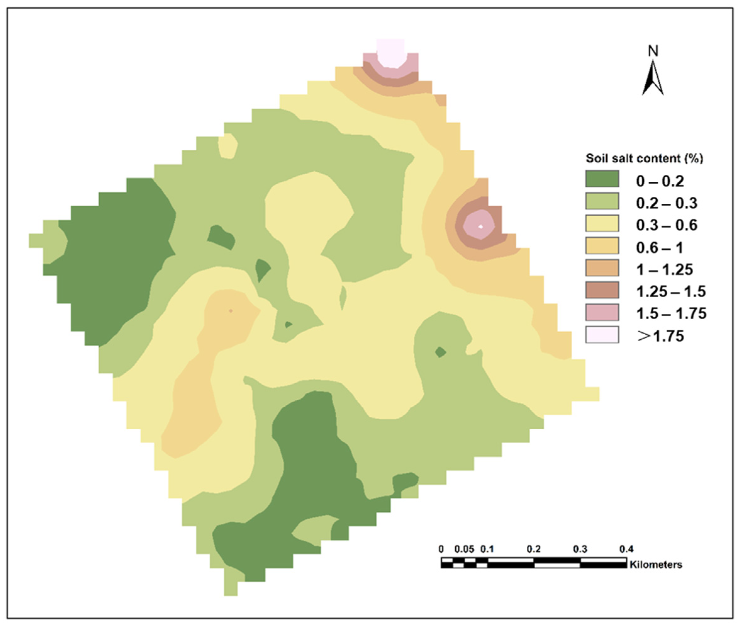
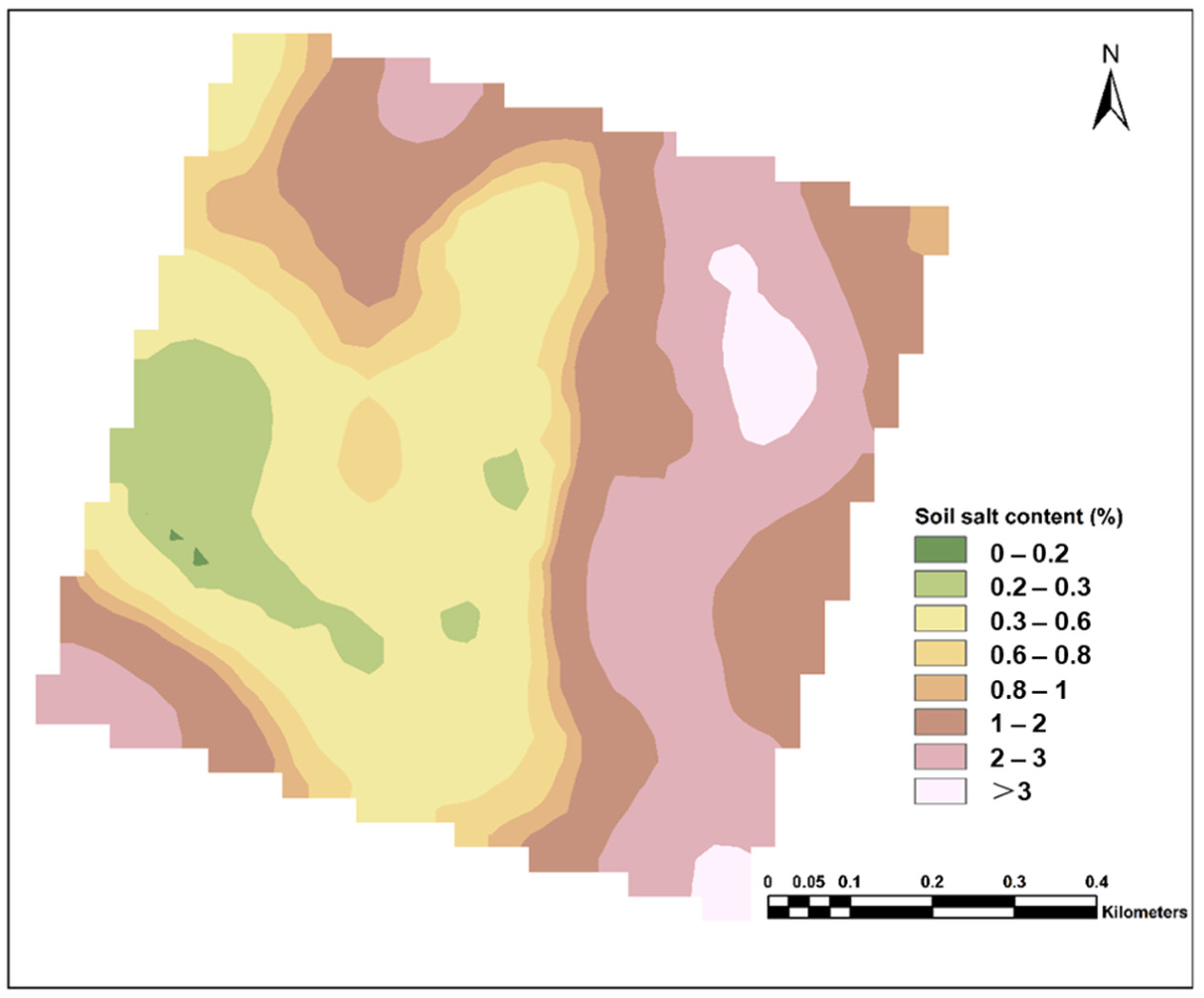
The analysis of the variance function structure of soil salinity and the results of Kriging interpolation are shown in Table 4 and Figure 3, respectively. The analysis of the variance function structure showed that the theoretical model of the soil salinity variance function in region N conformed to the exponential model, while that in region S conformed to the spherical model, but the R2 values of both models were higher, 0.82 and 0.97, respectively, which indicated that the selected model could fit the data better and accurately reflect the spatial variability characteristics of soil salinity at the sampling scale. The of soil salinity in the N and S regions was 41.27% and 19.46%, respectively. This indicated that the spatial variation in soil salinity in the N region was influenced by both random factors such as irrigation and cultivation practices and structural factors such as soil type, while in the S region, the spatial variation was mainly influenced by structural factors. The in the N and S regions was 603.00 m and 762.00 m, respectively, indicating that the soil salinity in both regions had a large spatial autocorrelation distance. This was due to the sampling period being during the drought period, where continuous and intense evaporation enhances the homogeneity of surface soil salinity distribution. It was also the fallow period, and agricultural activities, such as irrigation, fertilizer application, and cultivation activities, are relatively infrequent, which decreases the spatial autocorrelation of surface soil salinity during this period.

Table 4.
Soil salinity variance function model and its related parameters.

Figure 3.
Spatial distribution of soil salinity in the N study region.
From the spatial distribution of soil salinity (Figure 3 and Figure 4), the soil salt content in both the N and S regions exhibits a pattern of stripes and patches. In the N study region, the soil salinity is relatively low, and the land is mainly used for cultivating sunflowers. Therefore, microtopography, human activities, and other factors may be important factors contributing to this distribution pattern of salinity. In the S study region, soil salinity is higher and mainly concentrated in the eastern part of the study region, which is mainly due to the different land use patterns in the eastern and western parts of the S study region, with the eastern part being a saline wasteland, while the western part of the study region is mainly dominated by agricultural land. This difference in land use leads to variations in soil salinity distribution between the eastern and western regions.
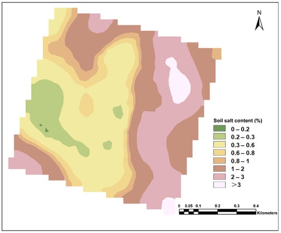
Figure 4.
Spatial distribution of soil salinity in the S study region.
4.3. Model Results and Analysis
Based on the salinity Kriging interpolation results described in Section 4.2, the ground “relative truth” value corresponding to the pixel scale was generated at a scale of 30 m. Subsequently, the generated pixel-scale “relative truth” was classified according to the salt-affected classification criteria, and the classified salt-affected degrees were used as the dependent variable for sensitive spectral feature selection and subsequent model construction. During the feature selection phase, the CFS method was employed to select features, resulting in the selection of the feature subset S1, S3, S7, and GAEX. Finally, the selected subset of features was used to construct salinization remote sensing monitoring models using the BC algorithm. In constructing the model, 70% of the total samples were used as the training set, and 30% were used as the validation set. In the following analysis, the models built based on single features are referred to as KDE-BC_S1, KDE-BC_S3, KDE-BC_S7, and KDE-BC_GAEX. The combination of a single-feature BC model using the EL concept is denoted as KDE-BC_EL, and the model confusion matrix results are shown in Appendix A Figure A1.
The single-feature constructed KDE-BC model was moderately successful in predicting soil salinity based on the evaluation scores of the model (recall, precision, F1-score), and the model results was shown Table 5. However, there are still some challenges. One noteworthy issue is that different KDE-BC models had varying scores when identifying the same soil salinity type. For example, when identifying saline soil, the F1-scores of KDE-BC_S1, KDE-BC_S3, KDE-BC_S7, and KDE-BC_GAEX were 0.82, 0.89, 0.57, and 0.84, respectively. The recall and precision patterns were similar to those of the F1-score. However, when combining the single-feature constructed KDE-BC models, it was found that KDE-BC_EL significantly improved the identification of various salinity types, indicating its good applicability in classifying salinization.

Table 5.
Scores of model evaluation metrics.
Further analysis of the model accuracy revealed that among the KDE-BC models, KDE-BC_S3 performed the best, with accuracy and Kappa values of 0.77 and 0.70, respectively. On the other hand, KDE-BC_S7 performed the worst, with accuracy and Kappa values of 0.66 and 0.55, respectively. In comparison to the KDE-BC model, KDE-BC_EL provided more accurate predictions, with accuracy and Kappa reaching 0.85 and 0.80, respectively. This validated the effectiveness of the soil salinization identification model constructed based on the concept of ensemble learning. Importantly, the KDE-BC_EL model only improved the accuracy by 0.08 compared to the best KDE-BC model. However, considering the F1 score, the KDE-BC_EL model effectively enhanced the robustness of the model.
5. Discussion
Soil salinity monitoring is crucial for land management in arid and semiarid regions. With the development and application of RS technology, unconventional monitoring of soil salinity has become possible, expanding the monitoring range of soil salt content beyond traditional techniques. However, due to the significant spatial heterogeneity of soil salinity, observation data from different scales often lack comparability. Therefore, this study focuses on the spatial heterogeneity of soil salinity information at the RS pixel scale. Eight sample plots (at a pixel scale of 30 m) were selected to examine the spatial variability of soil salinity. The variation coefficient of salt content within the eight sample plots was greater than 10%, indicating that using the salt content value from any single sampling point within a 30 m scale cannot represent the salt content situation within that scale. However, most existing studies are based on the assumption of spatial homogeneity of soil salinity, using ground-level salt content observation data as the “true value” for establishing salt content RS models and validating the rationality and accuracy of RS inversion products, without considering the representativeness of the ground point salinity observation data, which is somewhat unreasonable. In addition, to obtain ground-level “relative true values” corresponding to the pixel scale, the study adopted the ordinary Kriging method to interpolate the salinity. However, the effectiveness of different Kriging methods in salt content interpolation was not compared. Therefore, it is necessary to further explore other Kriging interpolation methods, such as cokriging and indicator Kriging.
Soil formation involves both environmental factors and human activities. Environmental factors include topography, climate, vegetation cover, and land use types, which can influence the physical, chemical, and biological properties of the soil. Human activities such as land reclamation, cultivation, fertilization, irrigation, and drainage may also alter the composition and characteristics of the soil, thereby affecting the spatial heterogeneity of soil salinity. Spatial heterogeneity is an inherent property of the spatial distribution pattern of soil salinity, encompassing heterogeneity in spatial composition, configuration, and relationships [50]. It reflects the complexity and variability of the spatial system. The spatial heterogeneity of soil salinity is shaped by the combined influence of structural and stochastic factors. Structural factors enhance spatial correlations within the same layer, while stochastic factors weaken spatial correlations, driving the system towards homogenization and uniformity [51]. This study reveals that the N and S study regions exhibit spatial heterogeneity in soil salinity. Compared to the N region influenced by both structural and stochastic factors, the S region, influenced by structural factors, exhibits stronger spatial variation induced by spatial autocorrelation.
It is generally believed that spatial variability is a natural characteristic of soil salinity itself, and regardless of the observation scale being large or small, the spatial variability of soil salinity objectively exists. The ability of remote sensing imagery to retrieve soil salinity varies with different resolutions. However, for the spatial distribution of soil salinity, a single-resolution remote sensing image is challenging to accurately represent. Moreover, there are differences in the optimal scale for the precise inversion of soil salinity spatial features and variations. In future research, it would be beneficial to better serve soil salinity remote sensing monitoring by analyzing the relationship between ground-level patchy salt content at different spatial scales and remote sensing data to select the optimal scale.
The spectral index method is the most popular method used in research when attempting to characterize the relationship between soil reflectance and soil salinity. Previous soil salinity studies have accumulated empirical evidence (spectral indices) for soil salinity identification and verified their validity and reproducibility [52]. RS modeling is a critical stage in salinity monitoring, and the choice of estimation method can greatly influence the final results. In recent years, researchers have increasingly favored the approach of EL or multi-model inference [53,54,55]. Therefore, this study introduces the EL concept for soil salinity identification, and the recall rate is used to quantify the advantages of each participating model. Consistent with other research findings, this study also found that the soil salinization identification model constructed using the EL concept outperforms single participating models in terms of prediction and is more robust in classifying different categories, resulting in satisfactory results. Compared to a single model, the ensemble of multiple models in this study compensated for any potential deficiencies or unreliable information in any single model and improved the robustness of the predictions. However, the homogeneous EL concept method used in this study only improved the classification accuracy by 0.08 compared to the best single participating model, which warrants further consideration. (1) The Bayesian statistical method is an unconventional classification method that has a unique advantage in mining complex data and can provide meaningful and interpretable relational models [56], which can adequately address the unclear correspondence between feature variables and target variables, as demonstrated by the classic example of the Iris flower dataset classification. Therefore, single participating models may also produce good results. (2) Previous research has mostly focused on ensembles of heterogeneous models [37,57,58]. Compared to ensembles of heterogeneous models, homogeneous model ensembles reduce training costs but may also reduce model diversity [32,59,60,61]. Therefore, in further research, it is necessary to explore the application of the heterogeneous EL concept in predicting soil salinity to better monitor soil salinization.
6. Conclusions
In this study, we focused on the spatial heterogeneity of soil salinity and explored the potential of an EL concept combining single-feature BC methods for soil salinity identification based on the acquisition of ground “relative truth” values at the pixel scale of RS. It was found that the scale effects resulting from the mismatch between ground-based “point” salinity data and remote sensing pixel-based “spatial” data need to be considered when performing RS inversion. The introduction of the EL concept improved the accuracy of soil salinity RS monitoring, with an overall accuracy of 0.85. Although the improvement in overall accuracy compared to the best KDE-BC model was only 0.08, there was a significant improvement in the identification of various salinization types (e.g., F1-score), effectively enhancing the robustness of the model. Therefore, it is highly recommended to explore the potential of the EL concept in soil salinization identification to develop reliable models for identifying salinized soils, as well as for further applications in quantitative RS monitoring of soil salinity.
Author Contributions
Conceptualization, H.C. and J.W.; methodology, H.C. and J.W.; software, H.C.; validation, H.C.; formal analysis, H.C.; investigation, C.X.; resources, H.C.; data curation, H.C. and H.C.; writing—original draft preparation, H.C.; writing—review and editing, H.C. and J.W.; visualization, H.C. and J.W.; supervision, J.W.; project administration, J.W.; funding acquisition, J.W. All authors have read and agreed to the published version of the manuscript.
Funding
This work was financially supported by the National Natural Science Foundation of China (Grant No. 52379047 and 52209067) and the National Key Research and Development Program of China (Grant No. 2021YFD1900804).
Data Availability Statement
Data are contained within the article.
Conflicts of Interest
The authors declare no conflicts of interest.
Appendix A
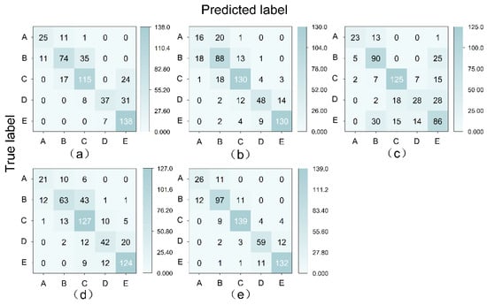
Figure A1.
Confusion matrix plots. A: Nonsaline, B: Slightly saline, C: Moderately saline, D: Strongly saline, E: Solonchak; (a) KDE-BC_S1, (b) KDE-BC_S3, (c) KDE-BC_S7, (d) KDE-BC_GAEX, (e) KDE-BC_EL.
Figure A1.
Confusion matrix plots. A: Nonsaline, B: Slightly saline, C: Moderately saline, D: Strongly saline, E: Solonchak; (a) KDE-BC_S1, (b) KDE-BC_S3, (c) KDE-BC_S7, (d) KDE-BC_GAEX, (e) KDE-BC_EL.

References
- Metternicht, G.I.; Zinck, J.A. Remote sensing of soil salinity: Potentials and constraints. Remote Sens. Environ. 2003, 85, 1–20. [Google Scholar] [CrossRef]
- Wang, J.; Zhen, J.; Hu, W.; Chen, S.; Lizaga, I.; Zeraatpisheh, M.; Yang, X. Remote sensing of soil degradation: Progress and perspective. Int. Soil Water Conserv. Res. 2023, 11, 429–454. [Google Scholar] [CrossRef]
- Farifteh, J.; Farshad, A.; George, R.J. Assessing salt-affected soils using remote sensing, solute modelling, and geophysics. Geoderma 2006, 130, 191–206. [Google Scholar] [CrossRef]
- Wang, J.; Ding, J.; Yu, D.; Teng, D.; He, B.; Chen, X.; Ge, X.; Zhang, Z.; Wang, Y.; Yang, X.; et al. Machine learning-based detection of soil salinity in an arid desert region, Northwest China: A comparison between Landsat-8 OLI and Sentinel-2 MSI. Sci. Total Environ. 2020, 707, 136092. [Google Scholar] [CrossRef] [PubMed]
- Abuelgasim, A.; Ammad, R. Mapping soil salinity in arid and semi-arid regions using Landsat 8 OLI satellite data. Remote Sens. Appl. 2019, 13, 415–425. [Google Scholar] [CrossRef]
- Wang, J.; Ding, J.; Ge, X.; Peng, J.; Hu, Z.W. Monitoring soil salinization based on remote sensing and proximal soil sensing: Progress and perspective. J. Remote Sens. 2023, 1–23. [Google Scholar] [CrossRef]
- Lobell, D.B.; Lesch, S.M.; Corwin, D.L.; Ulmer, M.G.; Anderson, K.A.; Potts, D.J.; Doolittle, J.A.; Motos, M.R.; Baltes, M.J. Regional-scale Assessment of Soil Salinity in the Red River Valley Using Multi-year MODIS EVI and NDVI. J. Environ. Qual. 2010, 39, 35–41. [Google Scholar] [CrossRef] [PubMed]
- Wang, J.; Ding, J.; Ma, X.; Zhang, Z.; Ge, X.; Lizaga, I.; Li, X.; Liang, J.; Chen, X.; Yuan, L.; et al. Capability of Sentinel-2 MSI data for monitoring and mapping of soil salinity in dry and wet seasons in the Ebinur Lake region, Xinjiang, China. Geoderma 2019, 353, 172–187. [Google Scholar] [CrossRef]
- Ge, X.; Ding, J.; Teng, D.; Wang, J.; Huo, T.; Jin, X.; Wang, J.; He, B.; Han, L. Updated soil salinity with fine spatial resolution and high accuracy. The synergy of Sentinel-2 MSI, environmental covariates and hybrid machine learning approaches. Catena 2022, 212, 106054. [Google Scholar] [CrossRef]
- Golestani, M.; Mosleh Ghahfarokhi, Z.; Esfandiarpour-Boroujeni, I.; Shirani, H. Evaluating the spatiotemporal variations of soil salinity in Sirjan Playa, Iran using Sentinel-2A and Landsat-8 OLI imagery. Catena 2023, 231, 107375. [Google Scholar] [CrossRef]
- Wang, L.; Hu, P.; Zheng, H.; Liu, Y.; Cao, X.; Hellwich, O.; Liu, T.; Luo, G.; Bao, A.; Chen, X. Integrative modeling of heterogeneous soil salinity using sparse ground samples and remote sensing images. Geoderma 2023, 430, 116321. [Google Scholar] [CrossRef]
- Abidine, M.M.O.; El Aboudi, A.; Kebd, A.; Aloueimine, B.B.; Dallahi, Y.; Soulé, A.; Vadel, A. Modeling the Spatial Variability of the Electrical Conductivity of the Soil Using Differents Spatial Interpolation Methods: Case of the Dawling National Park in Mauritania. Geogr. Tech. 2018, 13, 1–11. [Google Scholar] [CrossRef]
- Fu, T.; Gao, H.; Liu, J. Comparison of Different Interpolation Methods for Prediction of Soil Salinity in Arid Irrigation Region in Northern China. Agronomy 2021, 11, 1535. [Google Scholar] [CrossRef]
- Howari, F.M.; Goodell, P.C.; Miyamoto, S. Spectral properties of salt crusts formed on saline soils. J. Environ. Qual. 2002, 31, 1453–1461. [Google Scholar] [CrossRef]
- Cheng, L.; Aghakouchak, A.; Gilleland, E.; Katz, R.W. Non-stationary extreme value analysis in a changing climate. Clim. Chang. 2014, 127, 353–369. [Google Scholar] [CrossRef]
- Nie, M.; Huang, S.; Leng, G.; Zhou, Y.; Huang, Q.; Dai, M. Bayesian-based time-varying multivariate drought risk and its dynamics in a changing environment. Catena 2021, 204, 105429. [Google Scholar] [CrossRef]
- Yang, X.; Li, Y.P.; Huang, G.H.; Li, Y.F.; Liu, Y.R.; Zhou, X. Development of a multi-GCMs Bayesian copula method for assessing multivariate drought risk under climate change: A case study of the Aral Sea basin. Catena 2022, 212, 106048. [Google Scholar] [CrossRef]
- Davies, J.; Olley, J.; Hawker, D.; Mcbroom, J. Application of the Bayesian approach to sediment fingerprinting and source attribution. Hydrol. Process 2018, 32, 3978–3995. [Google Scholar] [CrossRef]
- Li, Y.; Gholami, H.; Song, Y.; Fathabadi, A.; Malakooti, H.; Collins, A.L. Source fingerprinting loess deposits in Central Asia using elemental geochemistry with Bayesian and GLUE models. Catena 2020, 194, 104808. [Google Scholar] [CrossRef]
- Fathabadi, A.; Jansen, J.D. Quantifying uncertainty of sediment fingerprinting mixing models using frequentist and Bayesian methods: A case study from the Iranian loess Plateau. Catena 2022, 217, 106474. [Google Scholar] [CrossRef]
- Wang, Y.; Zhao, T. Statistical interpretation of soil property profiles from sparse data using Bayesian compressive sampling. Géotechnique 2017, 67, 523–536. [Google Scholar] [CrossRef]
- Wang, C.; Li, X.; Zhang, J.; Liu, Y.; Situ, Z.; Gao, C.; Liu, J. Using Bayesian compressed sensing and sparse dictionaries to interpolate soil properties. Geoderma 2022, 428, 116162. [Google Scholar] [CrossRef]
- Luo, Y.; Weng, E.; Wu, X.; Gao, C.; Zhou, X.; Zhang, L. Parameter identifiability, constraint, and equifinality in data assimilation with ecosystem models. Ecol. Appl. 2009, 19, 571–574. [Google Scholar] [CrossRef]
- Heung, B.; Ho, H.C.; Zhang, J.; Knudby, A.; Bulmer, C.E.; Schmidt, M.G. An overview and comparison of machine-learning techniques for classification purposes in digital soil mapping. Geoderma 2016, 265, 62–77. [Google Scholar] [CrossRef]
- Tebaldi, C.; Knutti, R. The use of the multi-model ensemble in probabilistic climate projections. Philos. Trans. R. Soc. A 2007, 365, 2053–2075. [Google Scholar] [CrossRef]
- Baker, L.; Ellison, D. The wisdom of crowds—Ensembles and modules in environmental modelling. Geoderma 2008, 147, 1–7. [Google Scholar] [CrossRef]
- Peña, M.; van den Dool, H. Consolidation of Multimodel Forecasts by Ridge Regression: Application to Pacific Sea Surface Temperature. J. Clim. 2008, 21, 6521–6538. [Google Scholar] [CrossRef]
- Yan, J.; Sun, R.; Liu, T.; Duan, S. Domain-adaptation-based active ensemble learning for improving chemical sensor array performance. Sens. Actuators A-Phys. 2023, 357, 114411. [Google Scholar] [CrossRef]
- Taghizadeh-Mehrjardi, R.; Nabiollahi, K.; Minasny, B.; Triantafilis, J. Comparing data mining classifiers to predict spatial distribution of USDA-family soil groups in Baneh region, Iran. Geoderma 2015, 253–254, 67–77. [Google Scholar] [CrossRef]
- Kim, D.; Yu, H.; Lee, H.; Beighley, E.; Durand, M.; Alsdorf, D.E.; Hwang, E. Ensemble learning regression for estimating river discharges using satellite altimetry data: The Central Congo River as a Test-bed. Remote Sens. Environ. 2019, 221, 741–755. [Google Scholar] [CrossRef]
- Cimusa Kulimushi, L.; Bigabwa Bashagaluke, J.; Prasad, P.; Heri-Kazi, A.B.; Lal Kushwaha, N.; Masroor, M.; Mohammed, S. Soil erosion susceptibility mapping using ensemble machine learning models: A case study of upper Congo river sub-basin. Catena 2023, 222, 106858. [Google Scholar] [CrossRef]
- Pham, K.; Kim, D.; Park, S.; Choi, H. Ensemble learning-based classification models for slope stability analysis. Catena 2021, 196, 104886. [Google Scholar] [CrossRef]
- Taghizadeh-Mehrjardi, R.; Minasny, B.; Toomanian, N.; Zeraatpisheh, M.; Amirian-Chakan, A.; Triantafilis, J. Digital Mapping of Soil Classes Using Ensemble of Models in Isfahan Region, Iran. Soil. Syst. 2019, 3, 37. [Google Scholar] [CrossRef]
- Malone, B.P.; Minasny, B.; Odgers, N.P.; Mcbratney, A.B. Using model averaging to combine soil property rasters from legacy soil maps and from point data. Geoderma 2014, 232–234, 34–44. [Google Scholar] [CrossRef]
- Vaysse, K.; Lagacherie, P. Evaluating Digital Soil Mapping approaches for mapping GlobalSoilMap soil properties from legacy data in Languedoc- Roussillon (France). Geoderma Reg. 2015, 4, 20–30. [Google Scholar] [CrossRef]
- Rasaei, Z.; Bogaert, P. Spatial filtering and Bayesian data fusion for mapping soil properties: A case study combining legacy and remotely sensed data in Iran. Geoderma 2019, 344, 50–62. [Google Scholar] [CrossRef]
- Dasgupta, S.; Debnath, S.; Das, A.; Biswas, A.; Weindorf, D.C.; Li, B.; Shukla, A.K.; Das, S.; Saha, S.; Chakraborty, S. Developing regional soil micronutrient management strategies through ensemble learning based digital soil mapping. Geoderma 2023, 433, 116457. [Google Scholar] [CrossRef]
- Riggers, C.; Poeplau, C.; Don, A.; Bamminger, C.; Höper, H.; Dechow, R. Multi-model ensemble improved the prediction of trends in soil organic carbon stocks in German croplands. Geoderma 2019, 345, 17–30. [Google Scholar] [CrossRef]
- Song, X.; Wu, H.; Ju, B.; Liu, F.; Yang, F.; Li, D.; Zhao, Y.; Yang, J.; Zhang, G. Pedoclimatic zone-based three-dimensional soil organic carbon mapping in China. Geoderma 2020, 363, 114145. [Google Scholar] [CrossRef]
- Zhu, L.; Walker, J.P.; Shen, X. Stochastic ensemble methods for multi-SAR-mission soil moisture retrieval. Remote Sens. Environ. 2020, 251, 112099. [Google Scholar] [CrossRef]
- Nketia, K.A.; Asabere, S.B.; Ramcharan, A.; Herbold, S.; Erasmi, S.; Sauer, D. Spatio-temporal mapping of soil water storage in a semi-arid landscape of northern Ghana—A multi-tasked ensemble machine-learning approach. Geoderma 2022, 410, 115691. [Google Scholar] [CrossRef]
- Román Dobarco, M.; Arrouays, D.; Lagacherie, P.; Ciampalini, R.; Saby, N.P.A. Prediction of topsoil texture for Region Centre (France) applying model ensemble methods. Geoderma 2017, 298, 67–77. [Google Scholar] [CrossRef]
- Caubet, M.; Román Dobarco, M.; Arrouays, D.; Minasny, B.; Saby, N.P.A. Merging country, continental and global predictions of soil texture. Lessons from ensemble modelling in France. Geoderma 2019, 337, 99–110. [Google Scholar] [CrossRef]
- Castrignanò, A.; Buttafuoco, G. Geostatistical Stochastic Simulation of Soil Water Content in a Forested Area of South Italy. Biosyst. Eng. 2004, 87, 257–266. [Google Scholar] [CrossRef]
- Wu, J.; Vincent, B.; Yang, J.; Bouarfa, S.; Vidal, A. Remote Sensing Monitoring of Changes in Soil Salinity: A Case Study in Inner Mongolia, China. Sensors 2008, 8, 7035–7049. [Google Scholar] [CrossRef] [PubMed]
- Khan, N.M.; Rastoskuev, V.V.; Sato, Y.; Shiozawa, S. Assessment of hydrosaline land degradation by using a simple approach of remote sensing indicators. Agric. Water Manag. 2005, 77, 96–109. [Google Scholar] [CrossRef]
- Douaoui, A.E.K.; Nicolas, H.; Walter, C. Detecting salinity hazards within a semiarid context by means of combining soil and remote-sensing data. Geoderma 2006, 134, 217–230. [Google Scholar] [CrossRef]
- Allbed, A.; Kumar, L.; Aldakheel, Y.Y. Assessing soil salinity using soil salinity and vegetation indices derived from IKONOS high-spatial resolution imageries: Applications in a date palm dominated region. Geoderma 2014, 230–231, 1–8. [Google Scholar] [CrossRef]
- Taghizadeh-Mehrjardi, R.; Minasny, B.; Sarmadian, F.; Malone, B.P. digital mapping of soil salinity in Ardakan region, central Iran. Geoderma 2014, 213, 15–28. [Google Scholar] [CrossRef]
- Yang, Y.; Dou, Y.; Liu, D.; An, S. Spatial pattern and heterogeneity of soil moisture along a transect in a small catchment on the Loess Plateau. J. Hydrol. 2017, 550, 466–477. [Google Scholar] [CrossRef]
- Zhao, Y.; Feng, Q.; Yang, H. Soil salinity distribution and its relationship with soil particle size in the lower reaches of Heihe River, Northwestern China. Environ. Earth Sci. 2016, 75, 810. [Google Scholar] [CrossRef]
- Wang, Z.; Zhang, F.; Zhang, X.; Chan, N.W.; Kung, H.; Ariken, M.; Zhou, X.; Wang, Y. Regional suitability prediction of soil salinization based on remote-sensing derivatives and optimal spectral index. Sci. Total Environ. 2021, 775, 145807. [Google Scholar] [CrossRef] [PubMed]
- Liao, K.; Lai, X.; Zhou, Z.; Zhu, Q. Combining the ensemble mean and bias correction approaches to reduce the uncertainty in hillslope-scale soil moisture simulation. Agric. Water Manag. 2017, 191, 29–36. [Google Scholar] [CrossRef]
- Yao, Y.; Liang, S.; Li, X.; Chen, J.; Liu, S.; Jia, K.; Zhang, X.; Xiao, Z.; Fisher, J.; Mu, Q.; et al. Improving global terrestrial evapotranspiration estimation using support vector machine by integrating three process-based algorithms. Agric. For. Meteorol. 2017, 242, 55–74. [Google Scholar] [CrossRef]
- Zhang, R.; Xu, X.; Guo, J.; Sheng, Z. Multi-model ensemble approaches for simulation of evapotranspiration of karst agroforestry ecosystems. Agric. Water Manag. 2022, 273, 107869. [Google Scholar] [CrossRef]
- Zhao, K.; Wulder, M.; Hu, T.; Bright, R.M.; Brown, M.E. Detecting change-point, trend, and seasonality in satellite time series data to track abrupt changes and nonlinear dynamics: A Bayesian ensemble algorithm. Remote Sens. Environ. 2019, 232, 111181. [Google Scholar] [CrossRef]
- Chen, W.; Pourghasemi, H.R.; Kornejady, A.; Zhang, N. Landslide spatial modeling: Introducing new ensembles of ANN, MaxEnt, and SVM machine learning techniques. Geoderma 2017, 305, 314–327. [Google Scholar] [CrossRef]
- Zhang, Y.; Shen, F.; Sun, X.; Tan, K. Marine big data-driven ensemble learning for estimating global phytoplankton group composition over two decades (1997–2020). Remote Sens. Environ. 2023, 294, 113596. [Google Scholar] [CrossRef]
- Kuncheva, L.I.; Whitaker, C.J. Measures of Diversity in Classifier Ensembles and Their Relationship with the Ensemble Accuracy. Mach. Learn. 2003, 51, 181–207. [Google Scholar] [CrossRef]
- Akay, H. Spatial modeling of snow avalanche susceptibility using hybrid and ensemble machine learning techniques. Catena 2021, 206, 105524. [Google Scholar] [CrossRef]
- Sylvain, J.; Anctil, F.; Thiffault, E. Using bias correction and ensemble modelling for predictive mapping and related uncertainty: A case study in digital soil mapping. Geoderma 2021, 403, 115153. [Google Scholar] [CrossRef]
Disclaimer/Publisher’s Note: The statements, opinions and data contained in all publications are solely those of the individual author(s) and contributor(s) and not of MDPI and/or the editor(s). MDPI and/or the editor(s) disclaim responsibility for any injury to people or property resulting from any ideas, methods, instructions or products referred to in the content. |
© 2024 by the authors. Licensee MDPI, Basel, Switzerland. This article is an open access article distributed under the terms and conditions of the Creative Commons Attribution (CC BY) license (https://creativecommons.org/licenses/by/4.0/).

