Effectiveness of Management Zones Delineated from UAV and Sentinel-2 Data for Precision Viticulture Applications

Abstract

How accurately do Sentinel-2 (S2) images describe vine row spatial variability? Can they produce effective management zones (MZs) for precision viticulture? S2 and UAV datasets acquired over two years for different drip-irrigated vineyards in the Colli Morenici region (northern Italy) were used to assess the actual need to use UAV-NDVI maps instead of S2 images to obtain effective MZ maps. First, the correlation between S2 and UAV-NDVI values was investigated. Secondly, contingency matrices and dichotomous tables (considering UAV-MZ maps as a reference) were developed to compare MZ maps produced using S2 and UAV imagery. Moreover, data on grape production and quality were analyzed through linear discrimination analyses (LDA) to evaluate the effectiveness of S2-MZs and UAV-MZs to explain spatial variability in yield and quality data. The outcomes highlight that S2 images can be quite good tools to manage fertilization based on the within-field vigor variability, of which they capture the main features. Nevertheless, as S2-MZs with low and high vigor were over-estimated, S2-MZ maps cannot be used for high-accuracy input management. From the LDA results, the UAV-MZs appeared slightly more performant than the S2-MZs in explaining the variability in grape quality and yield, especially in the case of low-vigor MZs.

1. Introduction

Precision agriculture has seen remarkable advancements in recent years driven by the integration of different monitoring technologies, including satellites and unmanned aerial vehicles (UAVs) [1]. These tools enhance the ability to accurately describe within-field crop variability for applications aiming to optimize input supply and management practices while maintaining a sustainable production, as shown for viticulture by the authors of [2]. Indeed, this agricultural sector presents peculiar challenges due to the diversity of trellising systems employed, including both irrigated vine rows and rainfed inter-rows (with or without grass).

Among the different methodologies available for investigating within-field crop variability [3], multispectral and thermal remotely sensed imagery acquired from both satellite and UAVs proves to be very effective [4,5,6]. Both satellite and UAV data can describe a vineyard’s variability in space and time throughout the monitoring of its vegetative growth, though with very different time frequencies and spatial resolutions [2,7]. The time frequency for satellite data acquisition ranges from some days to one week (five days for Sentinel-2), and it can even fail in the case of a cloudy sky, while UAV data can be acquired on request, with very few limitations for weather conditions. Concerning their spatial resolution, it spans from tenths of meters (for Sentinel-2 and Landsat satellites) to a few centimeters (for UAVs). Thus, satellite and UAV imagery produces very different levels of detail in vineyard mapping [2,5]. Specifically for satellite data, reflectance and surface temperature measurements are collected over areas that can include both the vines (rows) and bare/grass-vegetated soils (inter-rows); consequently, satellite pixels are mixed (i.e., no or limited pure pixels can be found in the scene). Conversely, UAV imagery is characterized by centimetric pixels, which allow a precise identification of rows and inter-rows.

Moreover, sensors mounted on satellite and UAV platforms have very different spectral and optical properties, providing varying reflectance radiometric distributions and spectral resolutions. With the aim of exploiting both kinds of information from satellites and UAVs, many researchers have focused on their comparison and integration. In this context, a crucial point is how the vegetation indices (VIs), calculated from reflectance values measured in specific bands of different sensors and through the two platforms, can be compared. Many studies [7,8,9,10] show that NDVIs computed from UAV sensor bands are usually correlated with Sentinel-2 (S2)-derived indices, and are able to reproduce the spatial pattern in satellite images, though the absolute values can be significantly different, depending on the type of UAV sensor [7,8].

Ref. [9] found that maps of VIs for vineyards derived from S2 data are strongly correlated with those obtained from UAV data, at both the field and sub-field scale, and that S2 images can be effectively used for vineyard management instead of UAV images when high-spatial-resolution management is not the objective.

On the other hand, when a very-high-spatial-resolution field description is required, in particular for vineyards in which the canopy occupies less than 50% of the total area, it has been proven that the spatial patterns of the vine canopy and its vigor are described more accurately by high-resolution UAV images, especially in drip-irrigated vineyards [5,10]. In this case, the presence of a grass cover, bare soil, or shadows within the vineyard inter-rows can strongly affect the computation of the VIs derived from UAV imagery, as highlighted in [8].

It has been proven that S2 images mainly describe the variability in grass-covered inter-rows rather than that in vine rows, due to the pixel dimensions; consequently, the VIs calculated from S2 data generally show a higher correlation with unfiltered UAV data than with the filtered kind [5]. As a matter of fact, many processing methods have been developed to ‘filter’ pure canopy pixels from the background in the case of UAV imagery [5,11].

Vigor maps are used to delineate within-field zones with homogeneous characteristics for variable-rate management of mineral and/or hydric nutrition (i.e., management zones: MZs). One-year vigor maps can be used to define MZ maps for fertilization management, whereas time series of vigor maps should be used to produce MZs for variable-rate irrigation, since the environmental factors affecting grape production that are managed through variable-rate irrigation are mainly related to soil properties that have stationary spatial patterns of variability. MZs can be used also for selective harvesting, adopting different strategies based on the grape characteristics within each MZ, to potentially enhance production and wine quality [12,13,14]. Due to the mixed pixels, both soil and crop variability is expected to affect MZs derived from satellite imagery with medium resolution (like S2), leading to potentially different maps than those obtained from UAV imagery, which, given its centimetric-sized pixels, allows the selection of only the vine pixels to delineate MZs.

Finally, as spatial variability in a plant–soil system can lead to differences in the plant nutritional status and vigor, and consequently to different grape qualities and quantities [15], the within-field spatial heterogeneity of grape yield and quality could be investigated to understand its correspondence with delineated MZs that are used to manage the environmental factors of the plant–soil system affecting grape production [16].

This study aimed to assess the actual need to use UAV-NDVI maps instead of S2 imagery to obtain reliable and effective MZ maps for applications in precision viticulture, particularly for variable-rate fertilization. Indeed, refs. [5,10,17] proved that UAV data can more accurately describe the spatial variability in vine vigor. Nevertheless, this paper intends to show that MZs derived from S2 imagery could be reliable and ‘functional’ to explain the spatial variability in grape production and quality measurements, for some applications in variable-rate fertilization management.

For a few vineyards containing different vine types (Merlot, Chardonnay, Cabernet Sauvignon, and Traminer cultivars), situated in the ‘Colli Morenici’ region south of Lake Garda in northern Italy, this study compares MZs delineated from NDVI maps elaborated from UAV and S2 data acquired over two seasons. First, a correlation analysis was adopted to compare NDVI maps produced from S2 images and three different UAV datasets, based on all pixels, only row pixels, and only inter-row pixels, to assess how accurately S2 imagery can reproduce the spatial pattern of vine vigor. Secondly, the UAV and S2 MZ maps were compared in terms of: (i) the spatial distribution of the pixels belonging to the different MZs (by developing multi-cluster contingency matrices and dichotomous tables with UAV-MZ maps as the reference); (ii) a ‘functional’ assessment of the MZs, considering the correspondence between the MZs and the spatial variability in data on grape production and quality (via linear discriminant analyses). This ‘functional’ assessment in the comparison of UAV and S2 maps is a novelty introduced by this paper.

2. Materials and Methods

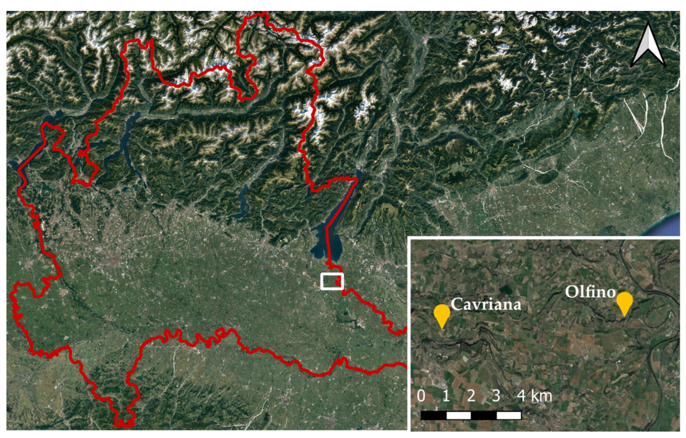
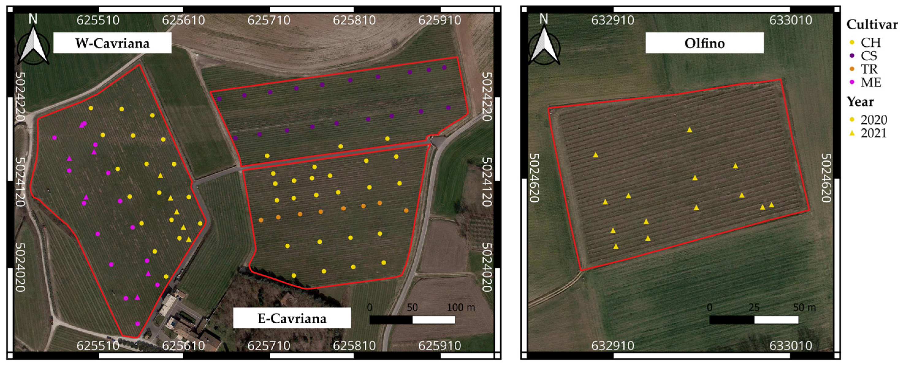
2.1. Experimental Sites

In this study, two experimental sites were considered: (i) a vineyard (field-scale site) situated in Olfino di Monzambano; (ii) a group of vineyards (farm-scale site) situated in Cavriana. These two sites are located about 10 km apart in the province of Mantova, northern Italy, in a hilly area named ‘Colli Morenici del Garda’ (Morainic Hills region) south of Lake Garda (Figure 1). Data were acquired and analyzed for the 2020 and 2021 seasons.

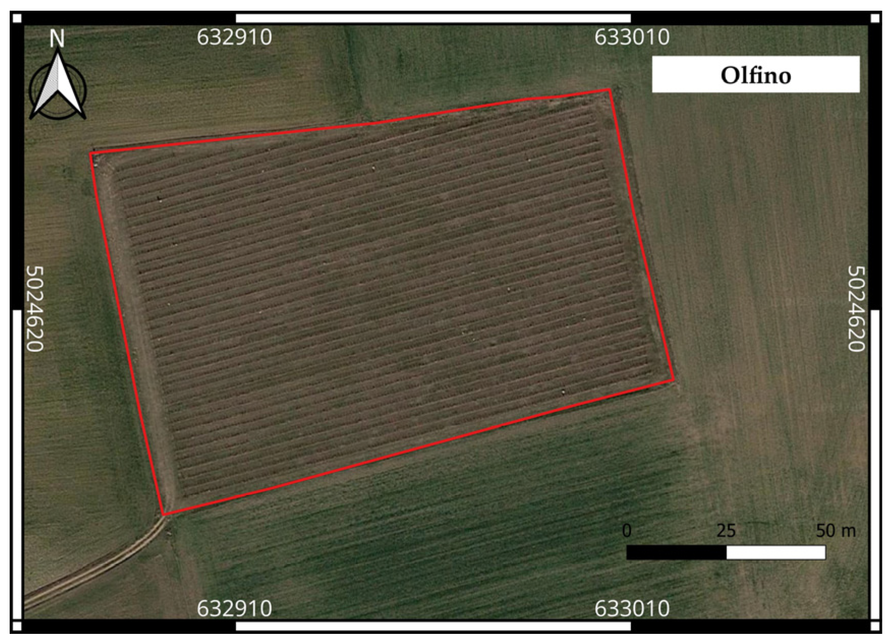
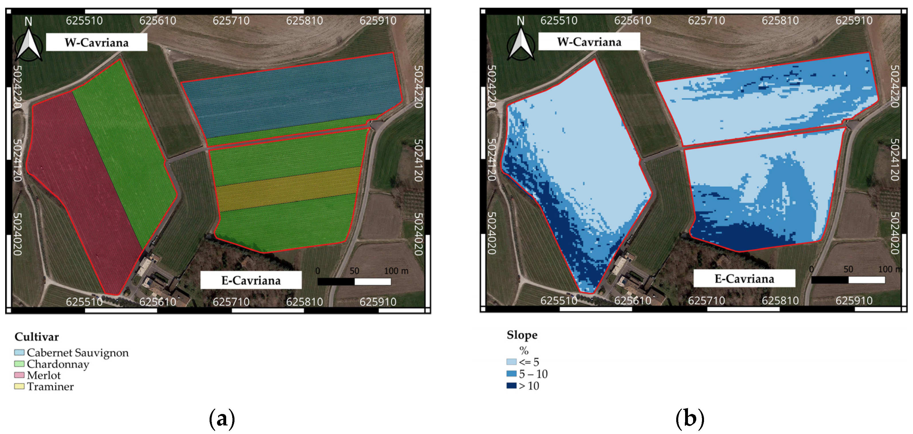
2.1.1. Field-Scale Site

The field-scale vineyard (Chardonnay cultivar) is situated in the ‘Cantina Gozzi’ farm. It is an almost flat 1 ha field (Figure 2). Vines are trained using a Guyot system, with the distance of vines on the row being 0.8 m, and the distance between rows being 2.4 m; the soil between rows is grass-covered with periodic mowing to avoid excessive grass growth, while the grass under the row is not mowed. A geophysical survey integrated with a pedological one conducted during a previous study showed that the field, despite its small area, is characterized by very different soil types [18]; in particular, soils in the western part of the vineyard are coarse and abundantly skeletal, while in the eastern part of the plot, soils show high percentages of silt and clay. Since 2018, the vineyard has been equipped with a variable-rate drip irrigation system with three sectors, each one with different dripper spacings and flow rates depending on the physical soil properties (texture and water retention); irrigation water is provided by the Garda-Chiese Irrigation Consortium with a 4 day turn; the irrigation management is optimized according to the actual soil water deficit measured through a monitoring network equipped with soil moisture sensors installed at two depths in one point within each sector. The harvest date for both experimental seasons was mid-August.

2.1.2. Farm-Scale Site

The farm-scale group of vineyards belongs to the ‘Azienda Agricola Ricchi’ and covers a total surface of about 10 ha. Unlike the site in Olfino di Monzambano, these vineyards are in a hilly area, where the topography is gently undulating. Three vineyards belong to this farm-scale site, with vines trained using a Guyot system, and grass-covered soil between rows. The westernmost field (hereafter referred to as ‘W-Cavriana’) is characterized by the presence of cultivars Merlot and Chardonnay (Figure 3a); in this field, the vine rows are arranged along the north–south axis, with a row spacing of about 2.6 m and a plant spacing on each row of 1 m. In the easternmost fields (hereafter named ‘E-Cavriana’), Cabernet Sauvignon is the prevailing variety in the northern part (except for few rows in the southern part of the field), while Chardonnay and Traminer cultivars are present in the southern vineyard (Figure 3a); the vine rows follow an east–west direction, with a row and plant spacing of 2.5 and 0.9 m, respectively. The site is characterized by steep areas with slopes exceeding 10% (Figure 3b).

According to the ERSAF pedological map (Lombardy pedological map 1:50,000, ERSAF), the vineyards rest on soil with the cartographic units 222 (loamy texture) and 229 (sandy loam at the surface, becoming loamy sand with depth). The results of a geophysical survey carried out in 2019 through an electromagnetic induction sensor [19] confirm their soil variability: in particular, the soils planted with Chardonnay cv within the W-Cavriana vineyard have a loamy texture, while the sandy-loam soils can be found in the portion of the vineyard that contains Merlot cv; in the E-Cavriana field, sandy-loam soils can be found in both vineyards. The whole farm-scale site is characterized by high percentages of gravel, varying across the three fields.

All the vineyards are equipped with a drip irrigation system with independent sectors; irrigation water was uniformly provided by a pumping well located in the farm, and the irrigation was managed according to the farmers’ expertise. The harvest for both the experimental seasons was in August for Chardonnay and Traminer cvs and in September for Merlot and Cabernet Sauvignon cvs.

2.2. UAV Surveys

Two UAV surveys were carried out in the years 2020–2021, during the phenological phase with maximum vine vigor (end of July). For both years, the flights were executed in clear sky days around 1 pm to minimize shadows; the flight directions were the same as the vine rows’ orientations, with nadiral acquisition of the frames.

Blocks of multispectral images were acquired according to the traditional photogrammetric scheme of parallel stripes, and with very-high overlaps both along tracks and across tracks (80–90%). The multispectral sensor, mounted on different UAVs (

Table 1. Setup for the UAV surveys.

Date	Dataset	UAV	Flying Height (m AGL)	Ground Control Points
20 July 2020	W-Cavriana E-Cavriana	Octocopter, self-assembled	60 m	10
23 July 2021	W-Cavriana Olfino	DJI Matrice 300	60 m 45 m	10 8

), was Micasense RedEdge (AgEagle Aerial Systems Inc., Wichita, USA) (

Table 2. UAV surveys: wavelengths of the multispectral sensor.

Sensor	Band	Wavelength (nm)
	Blue	475
Micasense	Green	560
RedEdge	Red	668
	Red Edge (RE)	717
	Near Infra-Red (NIR)	840

) for all surveys.

In 2020, the survey was conducted on the 20th of July, solely for the vineyards in the Cavriana site, with a self-assembled octocopter. The flight height was set to about 60 m above ground level (AGL). Ten Ground Control Points (GCPs) were positioned within the survey area [11]; 8 points were placed all around the boundary of the area and 2 were placed in the middle of the W-Cavriana and E-Cavriana fields, according to the procedure described in [11]. The positions of the 10 GCPs were measured with the Global Navigation Satellite System (GNSS) receiver Topcon GRS-1, in the Network Real-Time Kinematic (NRTK) mode to obtain a position accuracy of about ±2 cm. In 2021, the survey took place on the 23rd of July on both study sites, with a DJI Matrice 300 RTK. In the Olfino site, the drone flew at a height of 45 m AGL; 8 GCPs were used (7 positioned on the field boundary and 1 placed in the middle), whose positions were measured with the Topcon GRS-1 (accuracy: about ±2 cm). In the Cavriana site, the 2021 survey was carried out only for the W-Cavriana field; in this survey, the flight height was 60 m AGL and 10 GCPs were used, with the same setup used for the survey in 2020 (9 along the perimeter and 1 in the middle of each field), whose positions were measured with the Topcon GRS-1 (accuracy: about ±2 cm).

Images collected during the surveys were processed with Agisoft Metashape (version 2.0.3) software to obtain the Digital Surface Model (DSM) and the Digital Terrain Model (DTM), which were processed in QGIS to derive the Canopy Height Model (CHM), being the difference between the two. At the end of the photogrammetric processing, multispectral orthomosaics were produced for each survey, with a ground resolution of 3–4 cm/pixel, which were used to calculate the Normalized Difference Vegetation Index (NDVI) maps. To isolate the vine rows from the inter-row background, a threshold of 1.0 m was then applied to the CHMs in order to produce the sparse NDVI maps, with only the pixels corresponding to the vine rows or the inter-row background.

UAV surveys and their specifications are synthetized in Table 1 and Table 2.

2.3. Satellite Images

S2 Level-1C (top of the atmosphere reflectance) images from the Sentinel-2 archives were selected for dates as close as possible to the UAV flights. Only tiles with at most 20% cloud coverage were selected, with the chosen max cloud coverage of the area of interest at 0%. The images were downloaded and pre-processed by using the Sen2r package [20] of the R software (version 4.2.3) [21] for the atmospheric (sen2cor function) and topographic corrections, achieving Level-2A data (bottom of the atmosphere reflectance); finally, NDVI maps (Geotiff format) with 10 m spatial resolution were produced for the areas of interest. Precisely, the following images were considered: those acquired on 22 July 2020 for the W-Cavriana and E-Cavriana fields, and on 20 July and 22 July 2021 for, respectively, the Olfino and W-Cavriana fields.

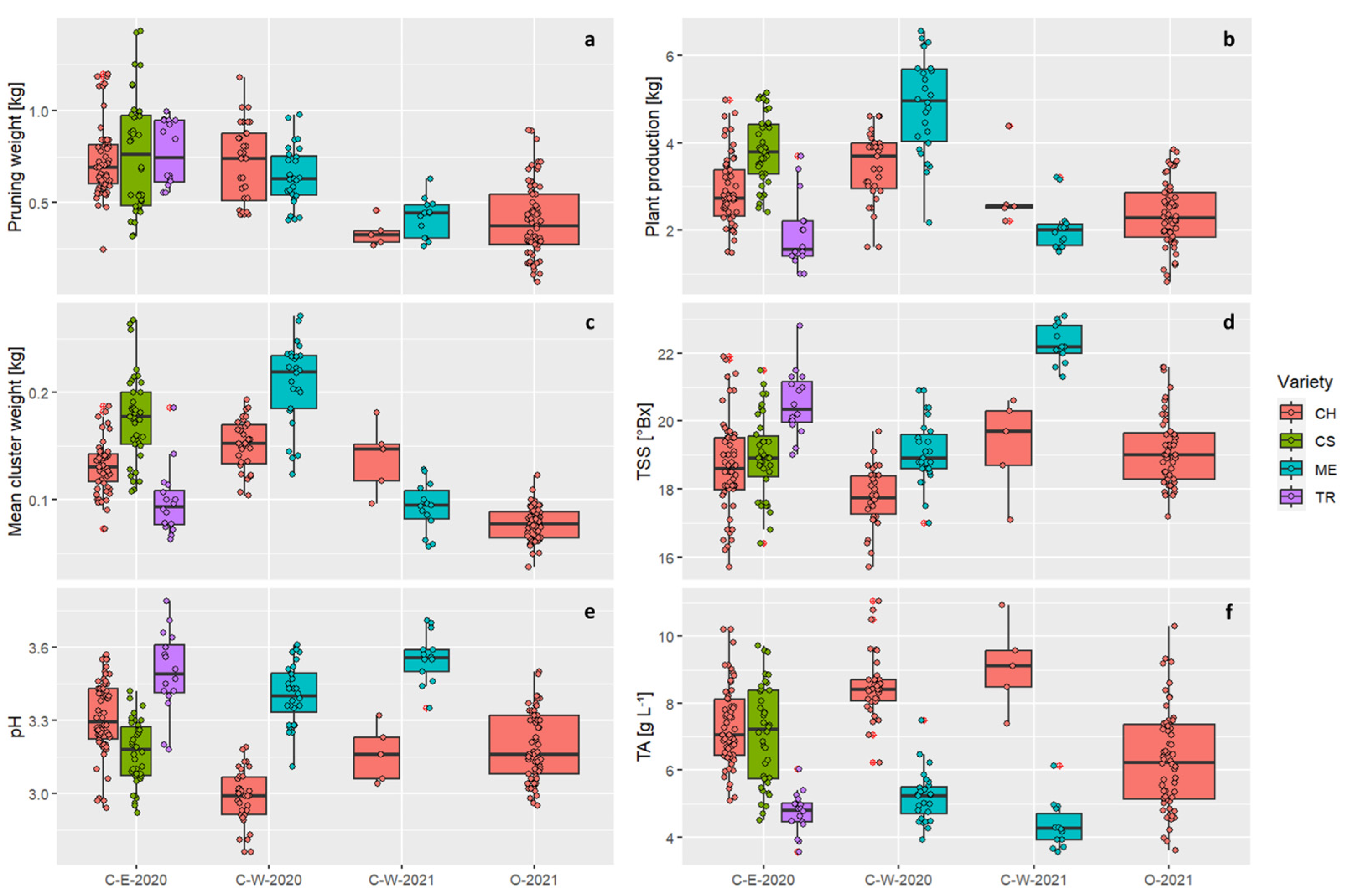
2.4. Vine Vigor, Grape Yield, and Quality Data

During the two experimental years, vine vigor, grape production, and grape quality were measured in several parcels within the fields. In 2020, a total of 84 parcels were analyzed for the vineyards in Cavriana, divided into 52 parcels in E-Cavriana and 32 parcels in W-Cavriana. In 2021, a total of 14 parcels were analyzed in the vineyard in Olfino and 11 parcels within the W-Cavriana field. The average distance between parcels was about 30 m. The positions of the parcels are reported in (Figure 4).

For each parcel, multiple vines were selected for direct measurements: two vines for the E-Cavriana and W-Cavriana sites, and four vines for the Olfino field. At harvest, the number of buds, shoots, and bunches of each selected vine were recorded and the total grape production per plant was weighed. Two bunches per vine were collected from central shoots and pressed to obtain the must. To prevent fermentation, 0.2‰ sodium azide (NaN₃, VWR, Radnor, USA) was added to each must. The pruning weight of the selected vines was measured during dormancy as an index of vine vigor. The mean cluster weight was calculated as the ratio between plant grape production and the relative number of bunches. The Ravaz index was calculated as the ratio between grape production per plant and the relative pruning weight.

The quality of the must was analyzed considering the total soluble solids (TSSs), pH, and titratable acidity (TA). TSSs were determined for the grapevine must via refractometry using a digital refractometer (DBR 35 SALT, Udine, Italy) and expressed as Brix (°Bx). Must pH and TA were detected using an automatic titrator (FLASH Automatic Titrator, Steroglass, Perugia, Italy). Briefly, 7.5 mL of juice for each sample was diluted to 50 mL with ultrapure water (resistivity > 18.2 MΩ.cm at 25 °C) for TA analysis. The samples were titrated with 0.1 M NaOH to a pH of 8.3. TA was expressed as g titratable acid/L.

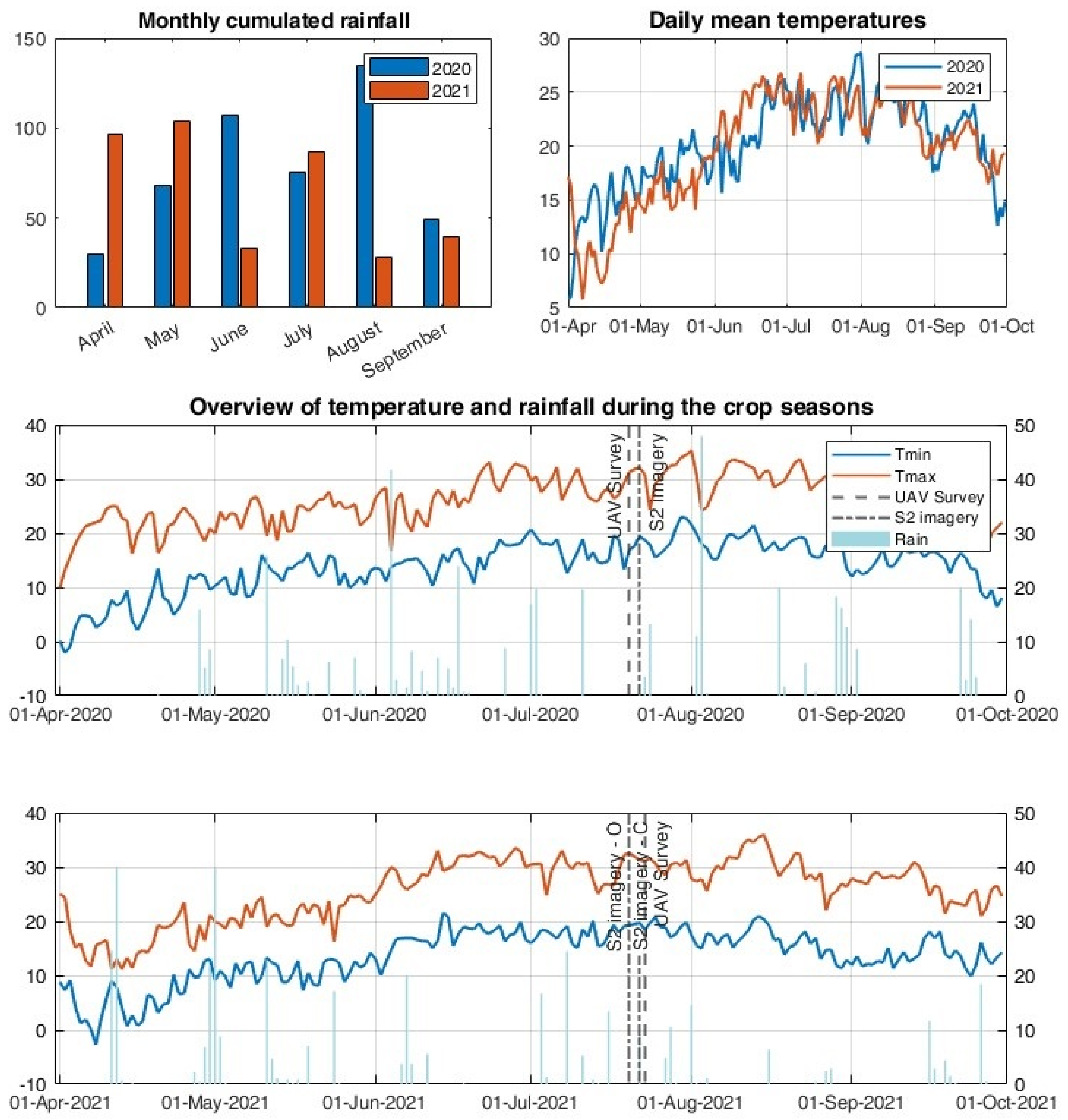
2.5. Agrometeorological Conditions in the 2020 and 2021 Seasons

The climate of the morainic hills of Garda is strongly influenced by the presence of Lake Garda, which has a mitigating effect on the temperatures of the area. Focusing on the study area, the meteorological variables for the years 2020 and 2021, recorded by an agro-meteorological weather station (MeteoSense, Netsens, Calenzano, Italy) located in the Olfino field, are reported in Figure 5. The climate in 2021 was characterized by higher rainfall and lower temperatures in spring with respect to 2020 (cumulated rainfall in April and May was 98 mm and 233 mm in 2020 and 2021, respectively, while daily mean air temperatures in the same two months differed by more than 2 degrees on average). On the contrary, June was colder and characterized by higher rainfall in 2020 than in 2021; starting from July, temperatures for both years became very similar, while rainfall in August was much higher in 2020.

In the last two panels of Figure 5, a general overview of the maximum and minimum temperatures and rainfall for both years is reported, together with the dates of the UAV surveys and the S2 imagery available for this study, which were chosen during the veraison (the phenological period most sensitive to water stress) and sufficiently far from rainfall, to emphasize the within-field vigor variability.

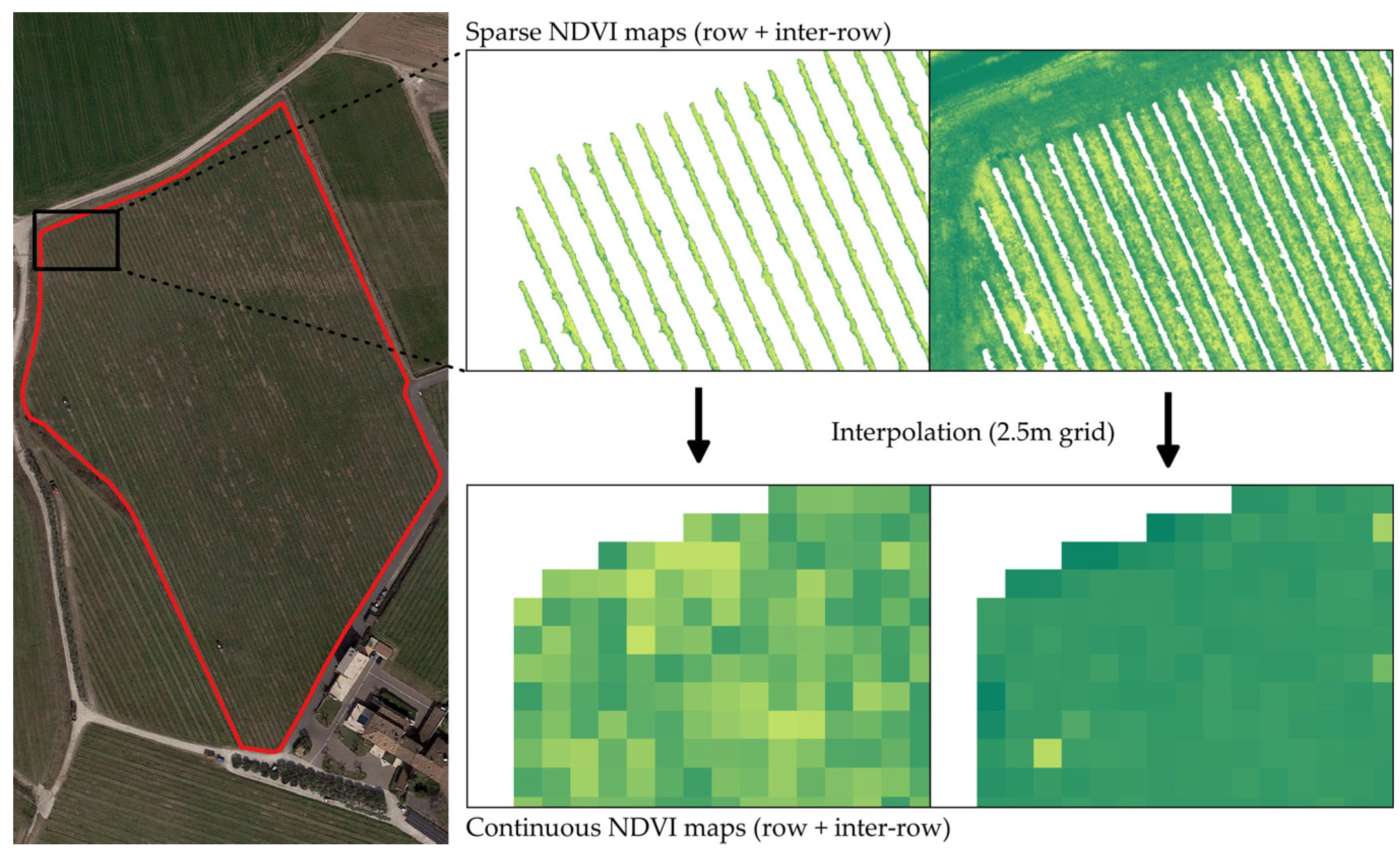
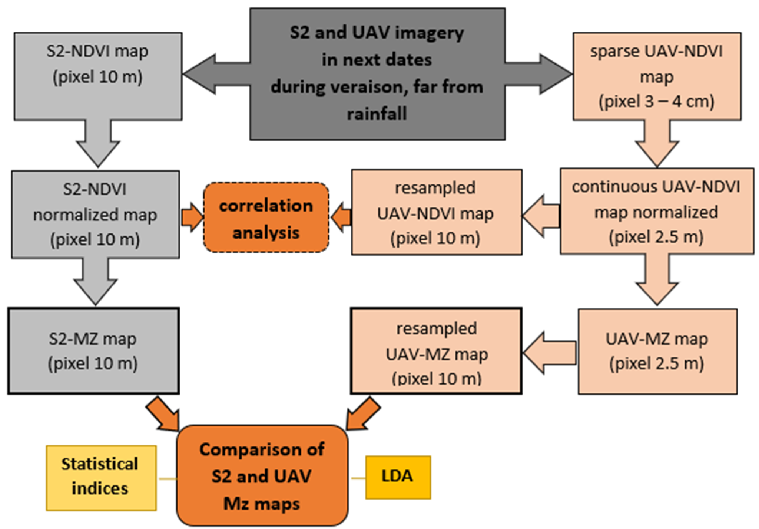
2.6. NDVI Maps from UAV and S2 Data

The spatial variability in vine vigor within the three experimental fields (i.e., Olfino, W-Cavriana, and E-Cavriana) was analyzed considering the NDVI maps at the end of July, during the veraison phenological phase. Because of the presence of different cultivars in the same field, and of different spatial resolutions for the S2 (10 m) and UAV (3–4 cm) data, the NDVI maps derived from UAV surveys (Section 2.2) were post-processed to produce final NDVI maps (as described below), from which the management zones (MZs) were delineated (Section 2.7).

First, the sparse UAV-derived maps, containing only row or inter-row pixels (Figure 6), were resampled onto 2.5 m pixel maps (comparable with the inter-row distance), in order to fill the null values obtained by removing the inter-row or row pixels, respectively; in this way, from the sparse NDVI maps with isolated pixels (3–4 cm sized), continuous NDVI maps with 2.5 m pixels were produced (hereafter referred to as ‘UAV-NDVI maps’).

Successively, in order to remove the effect of the presence of different cultivars in the same field on the spatial variability, both the UAV-NDVI maps and the S2-derived NDVI maps (hereafter named ‘S2-NDVI maps’) were normalized on grape cultivars: for each specific cultivar, the mean value was calculated from the NDVI values in all of the pixels with that cultivar, and the final NDVI maps (i.e., continuous maps with NDVI values normalized on grape cultivars) were produced according to the difference between the original NDVI value and the mean value. The variability in the vine vigor is then described through the quartiles of the distribution of the values in these final NDVI maps: the first and second quartiles (negative values) correspond to the pixels where the vine vigor is much less, and less than the mean value, for all cultivars; the third and fourth quartiles (positive values) correspond to the pixels where the vine vigor is greater, and much greater than the mean value, for all cultivars.

Comparison of NDVI Maps

Each couple of NDVI maps (with normalized values) obtained from UAV (with 2.5 m pixels) and S2 data acquired in almost the same dates was compared by calculating the correlation coefficients; for this aim, the UAV-NDVI values were resampled from the 2.5 m sized pixel to the 10 m sized pixel (S2 pixel dimension). The UAV-based maps including, in turn, all of the pixels, only the vine pixels, and only the inter-rows pixels, were considered; hence, for each couple of UAV and S2 maps, three correlation coefficients were obtained, hereafter named ‘UAV-S2’, ‘vine UAV-S2’, and ‘inter-row UAV-S2’, respectively. Moreover, the ‘vine UAV-S2*’ correlation index considered the S2 and UAV maps with normalized values.

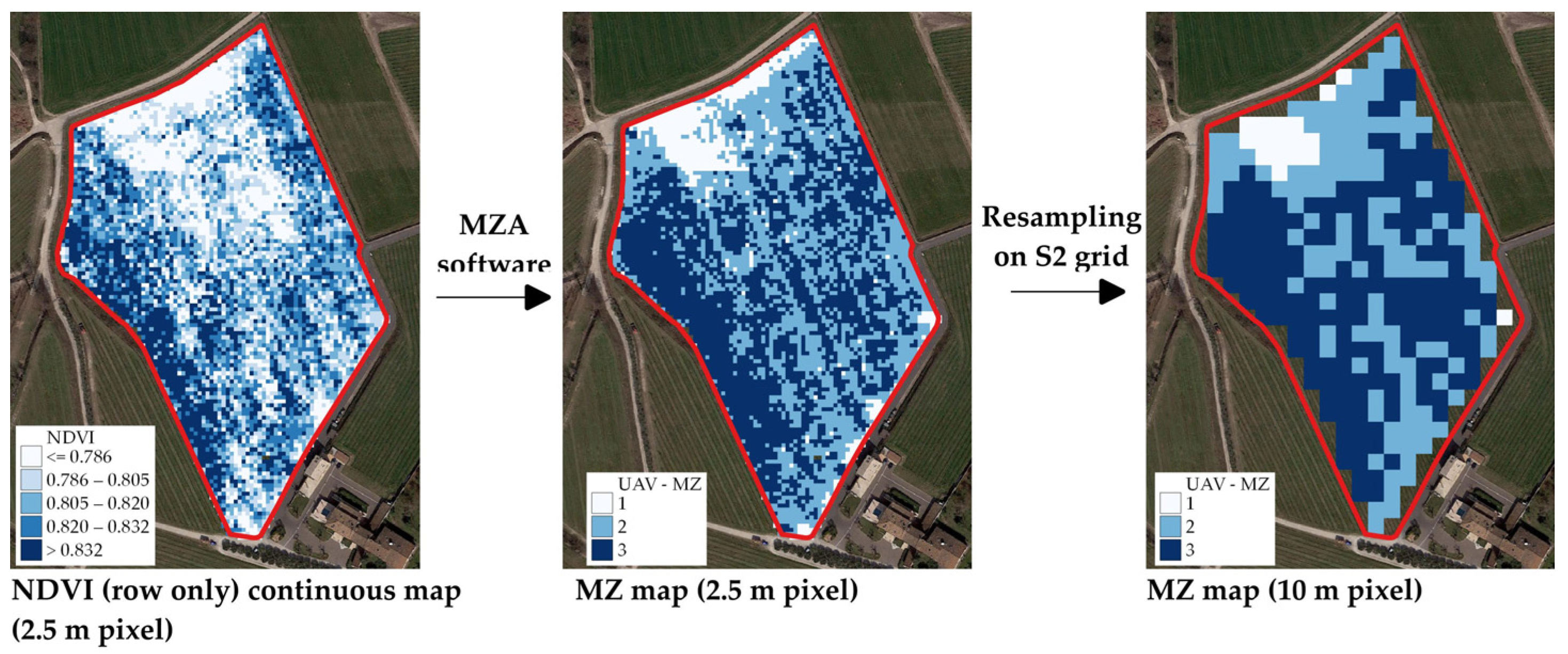
2.7. Delineation of MZs from NDVI Maps

The MZs were delineated through the Management Zone Analyst (MZA) software (version 1.0.1) [22], performing a k-means fuzzy unsupervised clustering on the final NDVI maps derived from S2 images and UAV data relative to only the vine rows (as defined in Section 2.6). The k-means algorithm minimizes the sum of squared Euclidean distances of all pixels from the cluster barycenter through successive iterations, adding pixels to clusters until a minimum is reached. The fuzzy approach consists of considering membership sharing between clusters for the boundary pixels, wherein the fuzziness exponent (m) controls these memberships: a value of 1 (i.e., no membership sharing) corresponds to hard clusters, while the clusters become less and less distinct with increasing m values; the default m value is set to 1.3. MZA determines the optimal number of MZs through the minimization of two indices: the Normalized Classification Entropy index (NCE) and the Fuzziness Performance Index (FPI), measuring, respectively, the degree of disorganization among MZs (the larger the NCE value, the higher the amount of disorganization) and the degree of separation between MZs (the larger the FPI value, the stronger the membership sharing between zones).

2.7.1. MZ Maps from UAV and S2 Data

In order to conduct a pixel-by-pixel comparison, due to the different pixel sizes of the final NDVI maps derived from UAV and S2 data (i.e., 2.5 m and 10 m, respectively), the MZ maps obtained from UAV data through the MZA software were referred to using the same grid and pixel dimension as that of the MZ maps obtained from S2 data. The following procedures were used to create the MZ maps for comparison. The MZ maps derived from S2 data (hereafter named ‘S2-MZ maps’) were obtained by processing the S2-NDVI maps directly in the MZA software, while the MZ maps from the vine UAV data (hereafter named ‘UAV-MZ maps’) were obtained through a two-step procedure (Figure 7): first, MZ maps with 2.5 m sized pixels were created through the MZA software; secondly, the latter maps were resampled on 10 m sized pixels, according to the majority criterion.

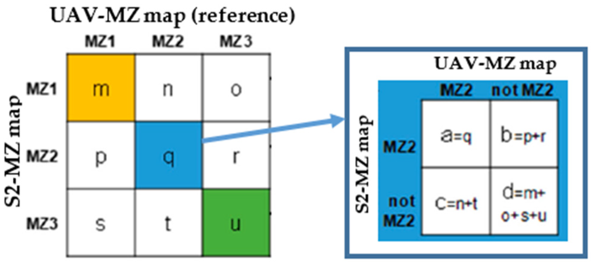
2.7.2. Comparison of MZ Maps

For each couple of MZ maps obtained from UAV and S2 data, the similarity was assessed by defining for each MZ the multi-cluster contingency matrix, and finally the dichotomous tables [23], by considering the UAV-MZ maps as the reference. Starting from the dichotomous tables, the following indices for each MZ were defined (Figure 8):

-

Proportion of Correct Classification (PCC) (equal to [a + d]/[a + b + c + d]), which is the proportion of correct classifications (i.e., pixels belonging/not belonging to a specific MZ) to the total number of pixels in the reference UAV-MZ map;

-

Hit rate (H) (equal to a/[a + c]), which represents the proportion of correct classifications (i.e., pixels belonging to a specific MZ) to the number of pixels belonging to that MZ in the reference UAV-MZ map;

-

Bias (BIAS) (equal to [a + b]/[a + c]), which is the ratio between the number of pixels belonging to a specific MZ in the S2-MZ map and those classified as belonging to that MZ in the reference UAV-MZ map, with no consideration of pixel position;

-

False Alarm Ratio (FAR) (equal to b/[a + b]), representing the proportion of pixels not correctly classified to the number of those belonging to a specific MZ in the S2-MZ map;

-

False detection (F) (equal to b/[b + d]), which is the ratio of pixels not correctly classified to the number of those not belonging to a specific MZ in the reference UAV-MZ map.

PCC and H increase up to the optimum value 1, with their minimum values depending on b and c; the optimum value for BIAS is 1, and its minimum and maximum values depend on b and c; FAR and F increase from the optimum value 0, with their maximum values depending on a and d, respectively. Finally, PCC was also globally defined (PCC = [m + q + u]/[all pixels in the reference map]), representing the proportion of pixels correctly classified for the different MZs in relation to the total number of pixels in the map.

2.8. Functional Evaluation of the MZ Maps

Data on vine vigor, grape quality, and production (Section 2.4) were analyzed using the R software (version 4.2.3) [21]. Particularly, boxplots were drawn using the ggplot2 package [24] to describe their variability. Moreover, a multivariate approach was used to classify the sampled vines according to the obtained MZs, in order to understand if the MZs can explain the data’s variability. Both the MZs obtained from UAV data and those obtained from S2 data were considered. A multivariate approach, considering data on the pruning weight, plant production, mean cluster weight, Ravaz index, TSSs, pH, and TA, was used to assess the NDVI MZs: a linear discriminant analysis (LDA) was independently performed for each field, year, and variety to find the contribution of each parameter in discriminating the MZs. In 2021, the variety Chardonnay in W-Cavriana was not considered for the LDA due to the limited number of vines sampled, all included in the same S2-MZ. One or two discriminant functions were built for each LDA, depending on the field, year, and variety. Coefficients of the discriminant functions were standardized to assess the contribution of each parameter in the LDA. The obtained discriminant functions were used to predict the belonging of each analyzed vine to the different NDVI MZs. Correct classification predictions with respect to the MZs delineated from UAV and S2 data were reported as percentages.

Figure 9 describes the analyses conducted.

3. Results

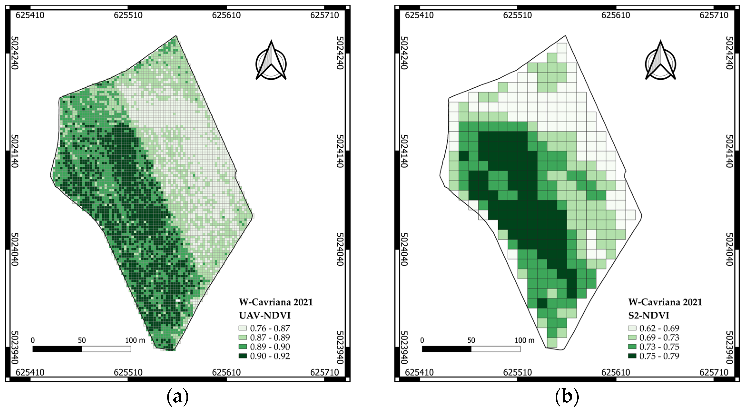
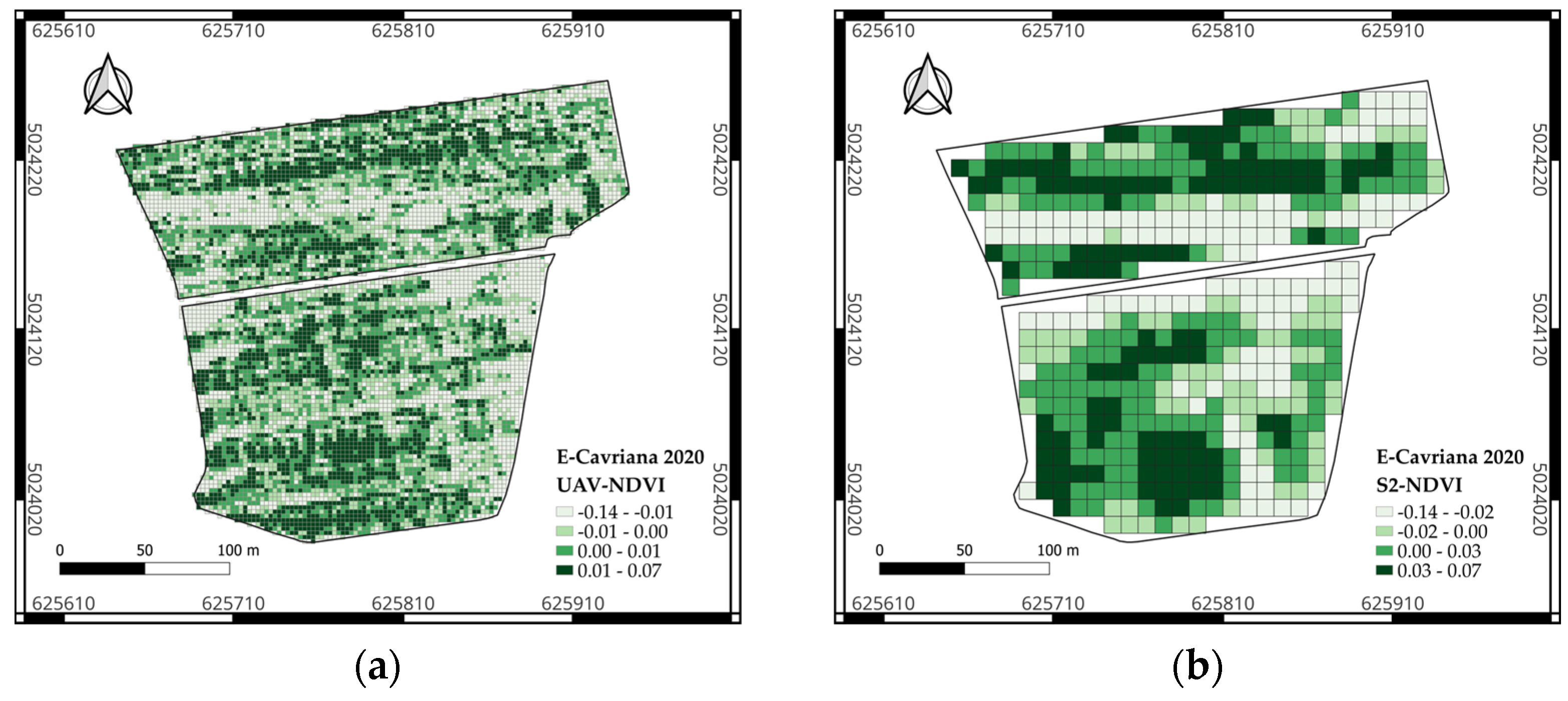
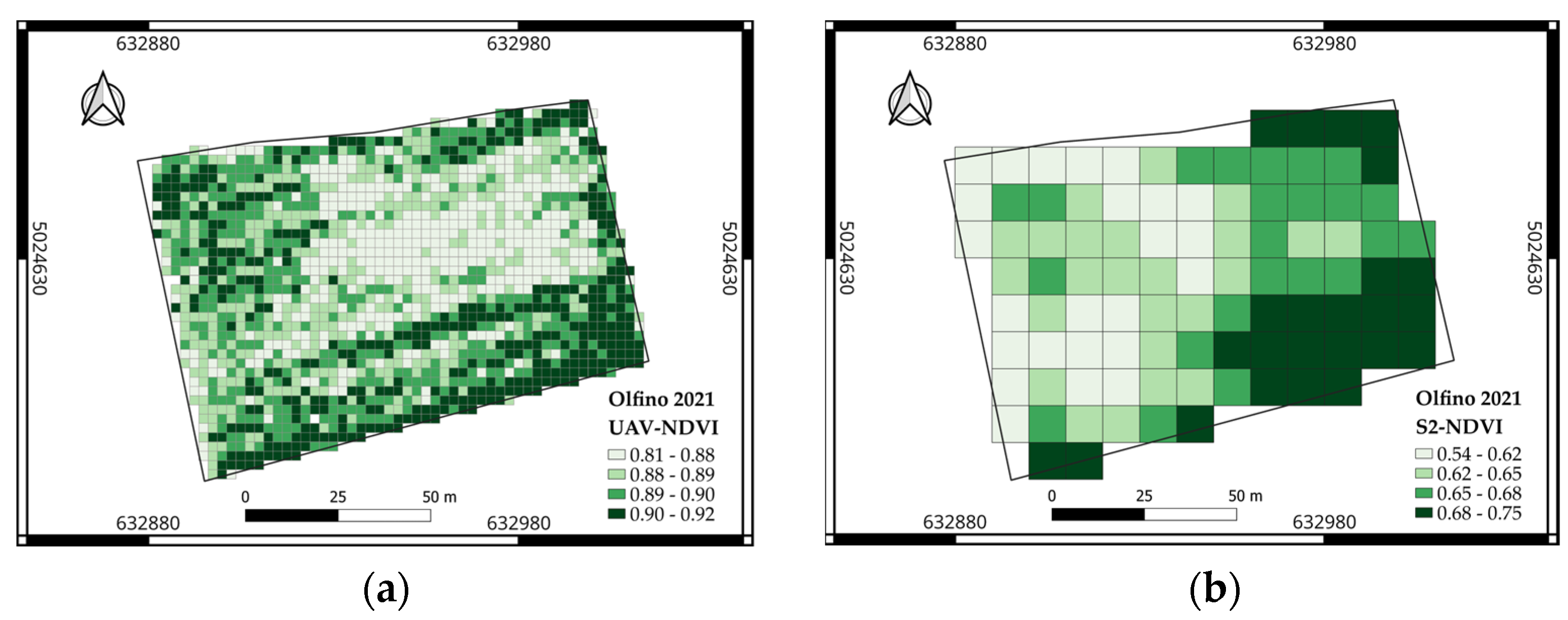
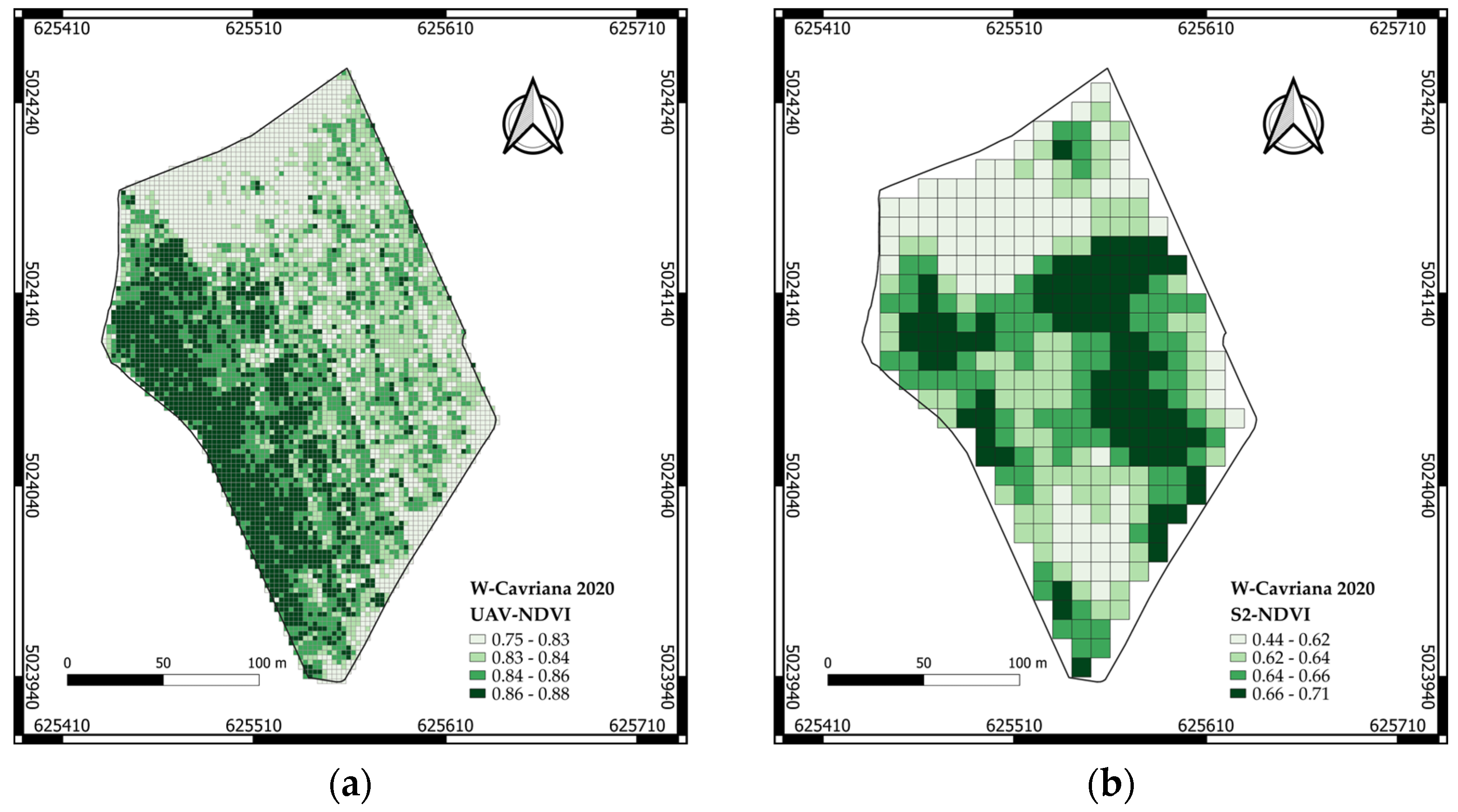
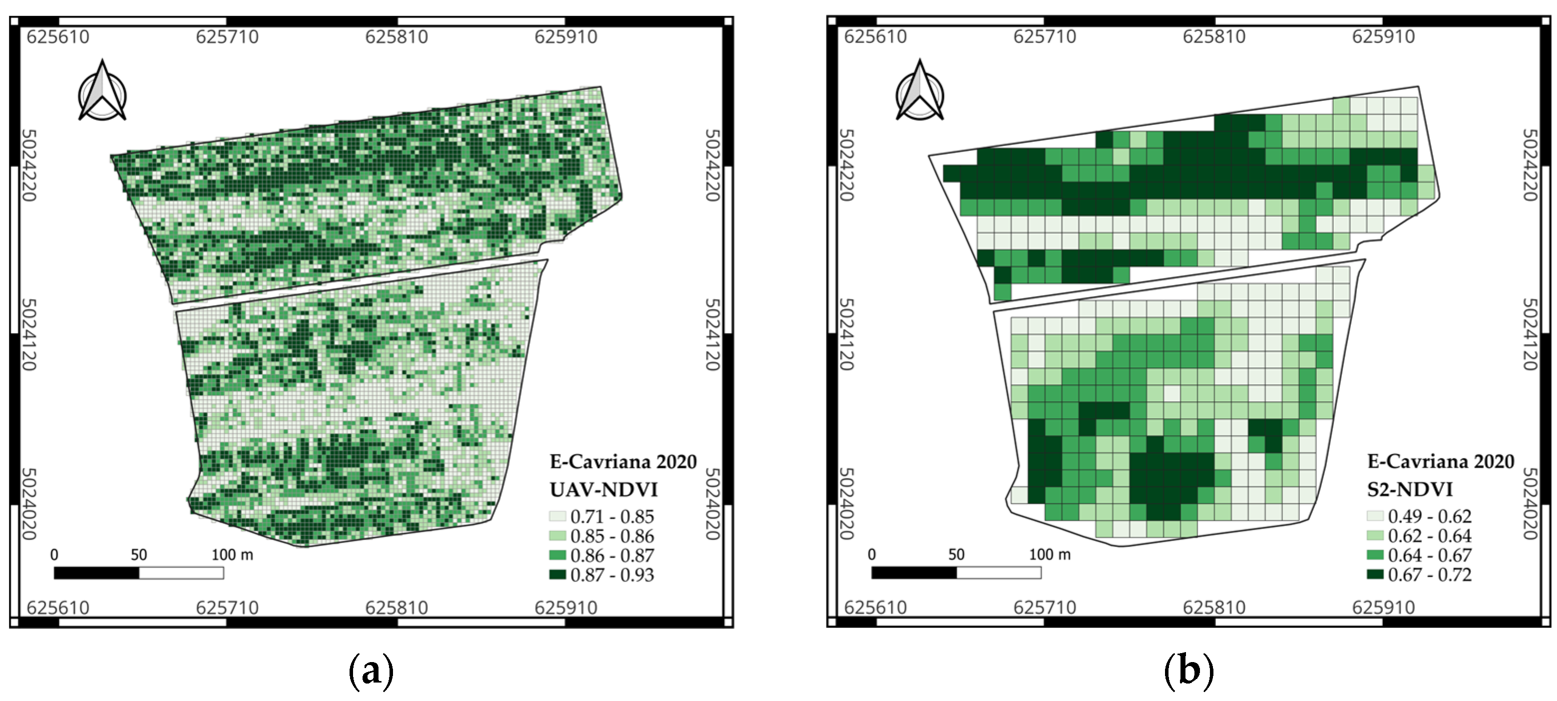
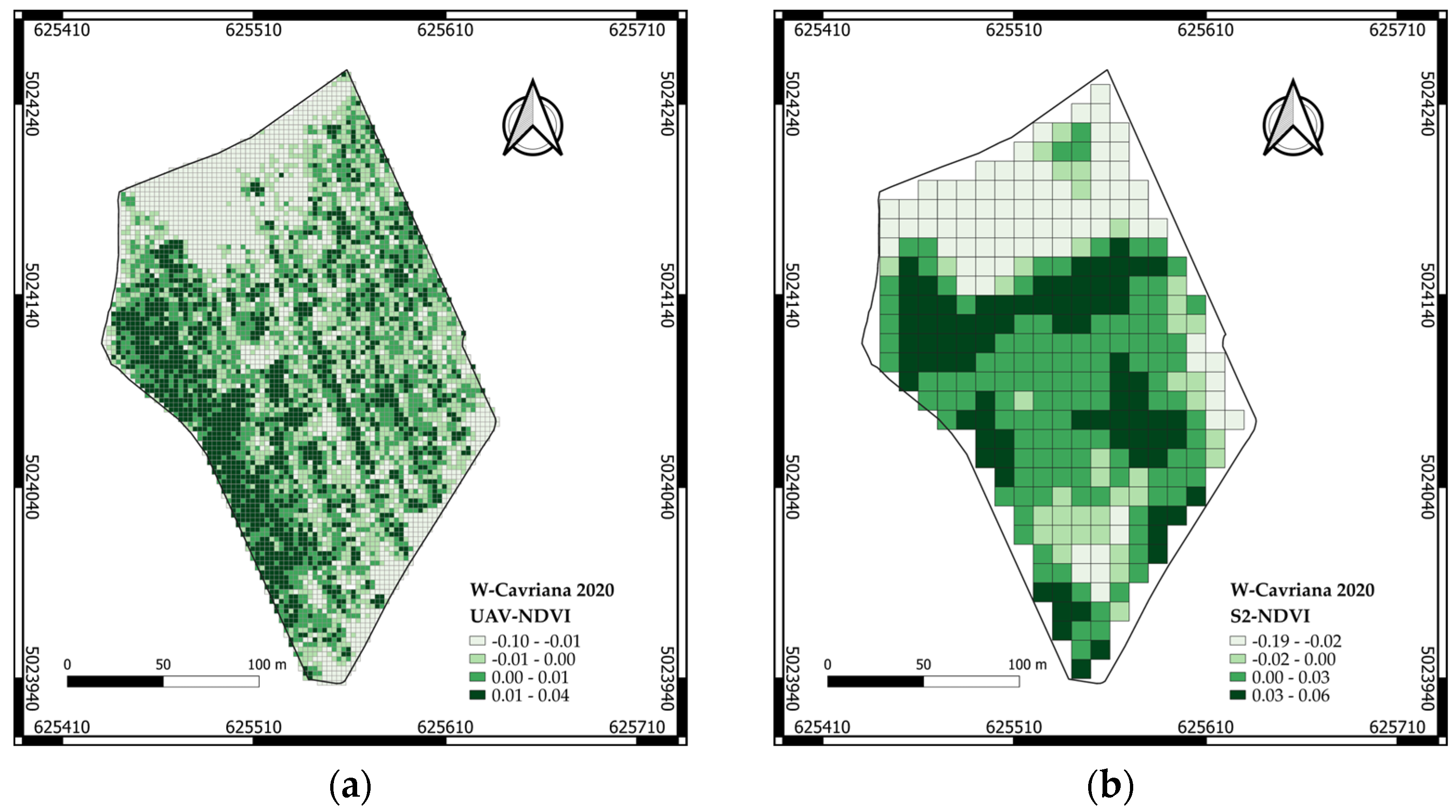
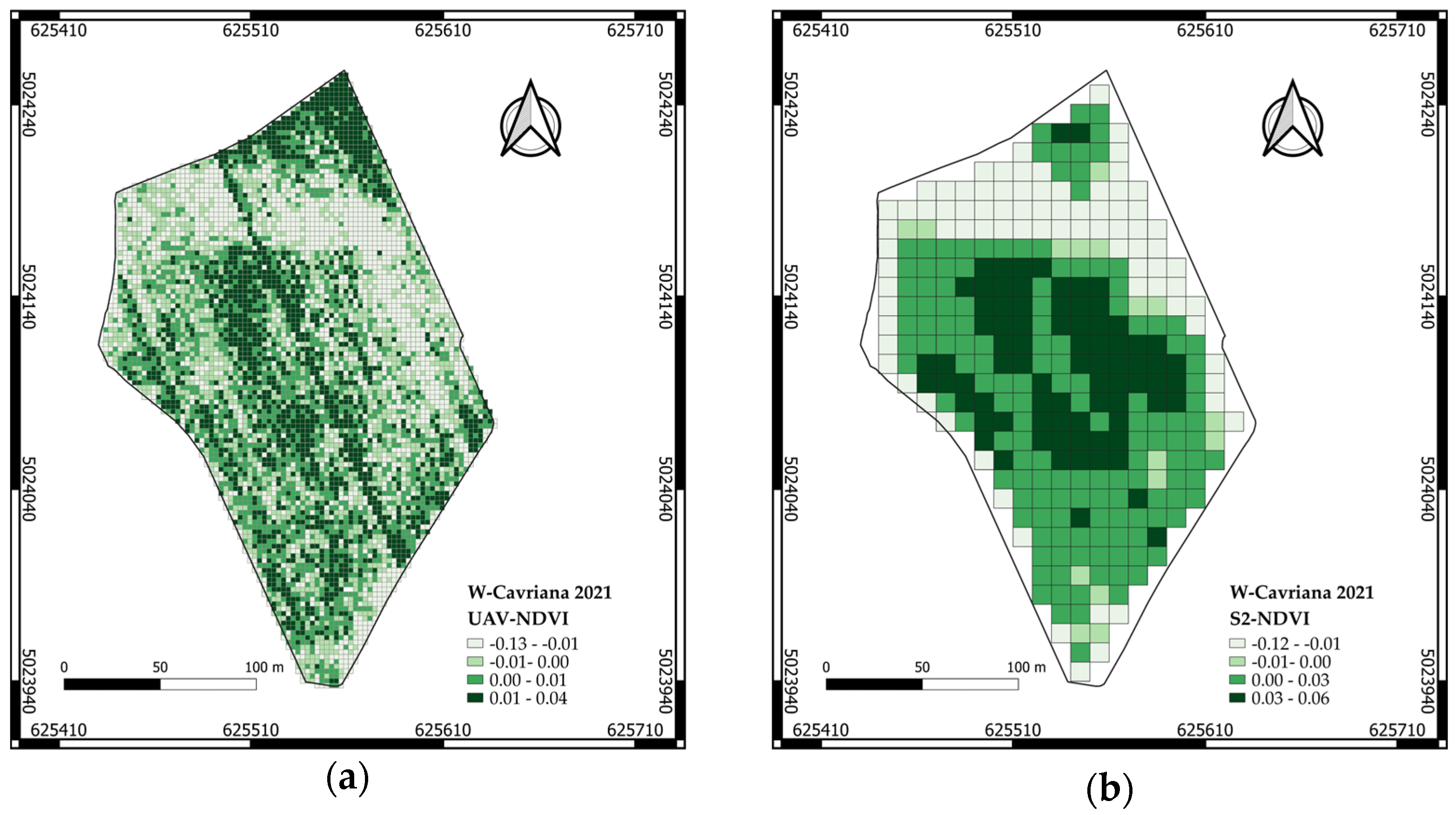
3.1. UAV-NDVI and S2-NDVI Maps

This section describes the S2-NDVI maps (10 m sized pixel) and UAV-NDVI maps (2.5 m sized pixel) considered in this study. The NDVI maps for the Olfino vineyard (July 2021) are shown in Figure 10, while Figure 11 and Figure 12 show the NDVI maps (July 2020) for the W-Cavriana and E-Cavriana fields, respectively, and Figure 13 describes the NDVI map (July 2021) for the W-Cavriana field. NDVI values for the 2020 season were generally lower than those for the 2021 season, probably due to the lower rainfall in April and May in 2020 (Figure 5).

Moreover, the S2-NDVI values were generally lower than the UAV-NDVI values, as the satellite pixels are mixed and provide information on the irrigated vine as well as on the grass-covered inter-row (not irrigated).

The normalized NDVI maps elaborated for the Cavriana site in the 2020 and 2021 (for only the W-Cavriana field) seasons are reported in Figure 14, Figure 15 and Figure 16. In all cases, the S2- and UAV-NDVI maps show comparable ranges of values.

Comparison between UAV-NDVI and S2-NDVI Maps

For each couple of UAV and S2 maps elaborated from data acquired on similar dates, the correlation coefficients between the S2-NDVI values and the UAV-NDVI values, obtained by resampling the S2 pixel dimensions onto 2.5 m sized pixels corresponding to the distance between the vine rows, were reported in

Table 3. Correlation coefficients between the S2-NDVI values and the UAV-NDVI values for each couple of UAV and S2 maps acquired on similar dates: ‘UAV-S2’, ‘vine UAV-S2’, and ‘inter-row UAV-S2’ values consider, respectively, all of the UAV pixel values, only the vine ones, and only the inter-row ones. For the maps with the normalized NDVI, only the ‘vine UAV-S2*’ values are illustrated.

Correlation Coefficient	W-Cavriana, 2020	E-Cavriana, 2020	W-Cavriana, 2021	Olfino, 2021
UAV-S2	0.68	0.51	0.86	0.74
inter-row UAV-S2	0.71	0.48	0.85	0.74
vine UAV-S2	0.43	0.39	0.75	0.50
vine UAV-S2*	0.70	0.40	0.55	-

. The coefficient values highlight the poor correlation: the ‘vine UAV-S2’ values reach a maximum of 0.50, and are always less than the ‘inter-row UAV-S2’ ones. Only the 2021 maps for the W-Cavriana field show a good correlation (‘vine UAV-S2’ value equal to 0.75), though always less than the ‘inter-row UAV-S2’ correlation coefficient (0.85). Moreover, the ‘inter-row UAV-S2’ correlation values are always comparable to the ‘UAV-S2’ ones, meaning that the S2-NDVI values are mostly affected by the NDVI of the grass-covered inter-row rather than the vine. Finally, the ‘vine UAV-S2*’ values, which are the correlation coefficients calculated for the maps with the normalized NDVI, were coherent with those obtained for the ‘vine UAV-S2’ coefficients (almost the same values or lower ones).

3.2. Delineation of MZs from NDVI Maps

The optimal numbers of MZs for each case, defined based on the FPI and NCE values, are reported in

Table 4. Optimal number of MZs for each NDVI map, based on the FPI and NCE values processed by the MZA software.

Optimal No. of MZs	W-Cavriana, 2020	E-Cavriana, 2020	W-Cavriana, 2021	Olfino, 2021
UAV-NDVI map	2	3	3	4
S2-NDVI map	4	3	2	4

. Since they sometimes are different for the couples of S2 and UAV-MZ maps (as for the W-Cavriana field in both 2020 and 2021), making comparison results difficult to evaluate, the delineation of three MZs (corresponding to low-, medium-, and high-vigor classes) was decided for all cases.

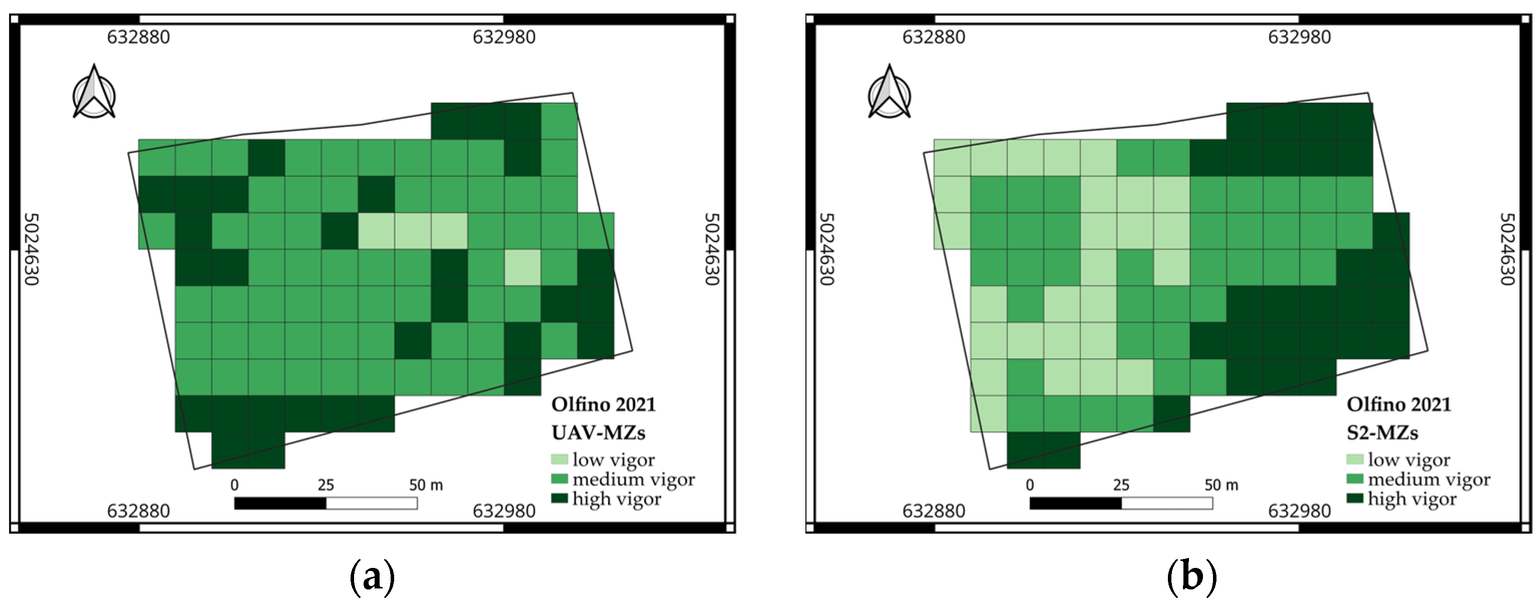
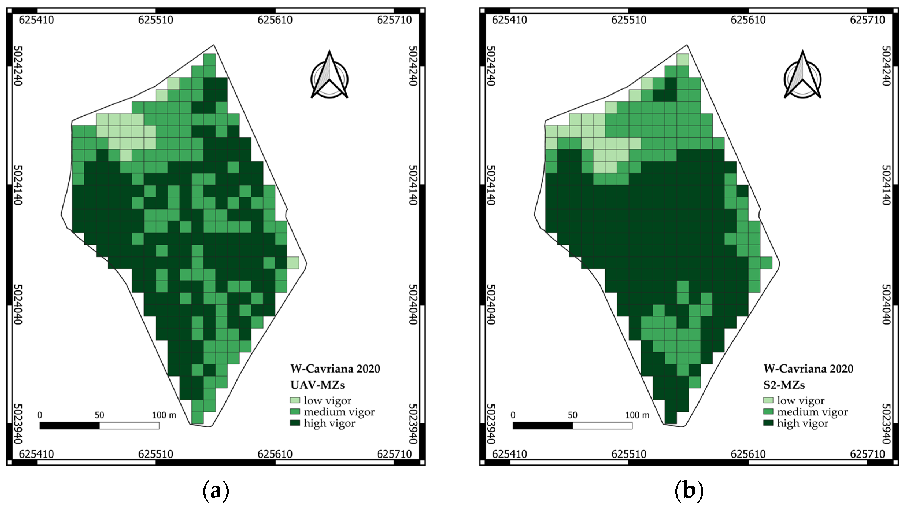
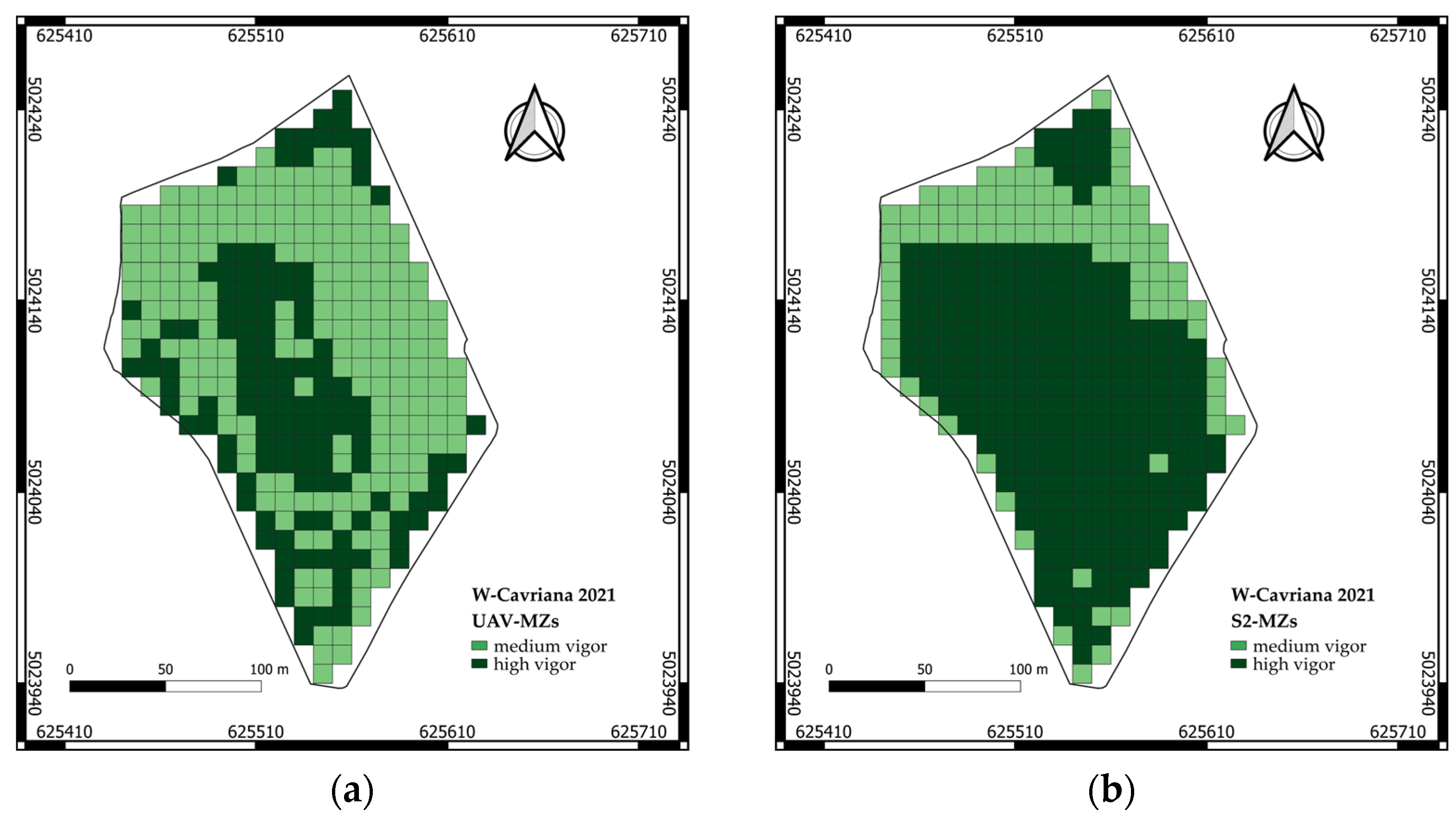
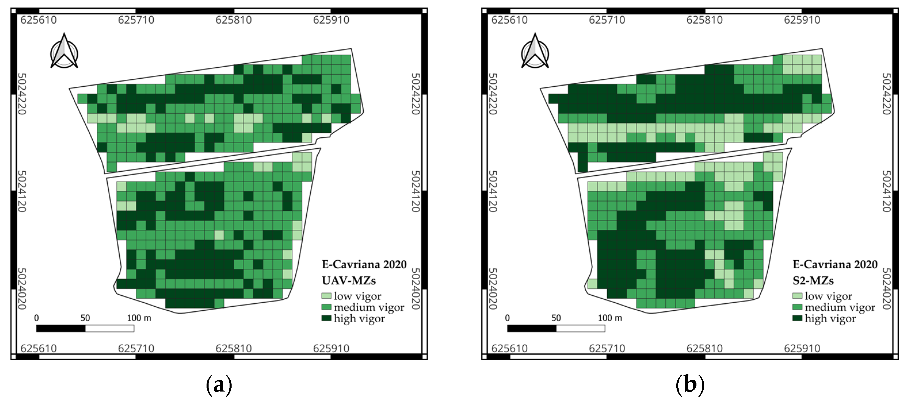
3.2.1. The UAV-MZ and S2-MZ Maps

Figure 17, Figure 18, Figure 19 and Figure 20 show MZ maps computed considering three zones; the number of MZs is reduced to two for the W-Cavriana field in July 2021 (Figure 19), since one zone was characterized by very few pixels (less than ten) in both the S2-MZ and UAV-MZ maps; in this case, the remaining zones correspond to medium- and high-vigor classes.

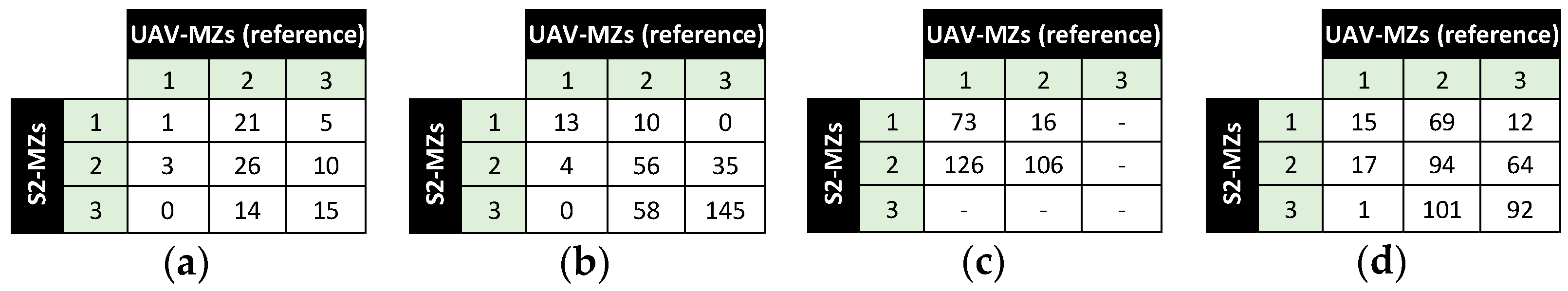
3.2.2. Comparison between UAV-MZ and S2-MZ Maps

Figure 21 describes the contingency matrices for each couple of considered UAV-MZ and S2-MZ maps (UAV-MZ maps are the reference ones), wherein the indices defined in Section 2.7.2 were calculated (

Table 5. Indices used to compare each MZ from the UAV-NDVI and S2-NDVI maps: ‘A’: W-Cavriana field, late July 2020; ‘B’: E-Cavriana field, late July 2020; ‘C’: W-Cavriana field, late July 2021; ‘D’: Olfino vineyard, late July 2021. Also, the global PCC is reported for each couple of maps.

Vigor Class	Low (MZ-1)				Medium (MZ-2)				High (MZ-3)
Index	A	B	C	D	A	B	C	D	A	B	C	D
PCC	0.96	0.79	-	0.70	0.67	0.46	0.56	0.50	0.71	0.62	0.56	0.70
H	0.77	0.46	-	0.25	0.45	0.36	0.37	0.43	0.81	0.55	0.87	0.50
BIAS	1.35	2.91	-	6.75	0.77	0.66	0.45	0.64	1.13	1.16	1.90	0.97
FAR	0.44	0.84	-	0.96	0.41	0.46	0.18	0.33	0.29	0.53	0.54	0.48
F	0.03	0.19	-	0.29	0.20	0.40	0.13	0.38	0.41	0.34	0.63	0.22
Global Index	A	B	C	D
PCC	0.67	0.43	0.56	0.44

).

The MZs with low and high vigor derived from S2 data were, respectively: heavily over-estimated for cases B and D (BIAS greater than 2), and over-estimated for cases A, B, and C (BIAS from 1 to 2); the BIAS value for the MZ with high vigor is almost optimum for case D; the MZ with medium vigor is always under-estimated (BIAS less than 1). FAR values of about 1 correspond to the maximum BIAS values, while the remaining FAR values, generally less or slightly higher than 0.50, are not proportional to BIAS values: in fact, the BIAS index does not consider the pixel position, while FAR states how many pixels of a specific MZ in an S2-MZ map do not correspond (depending on their position) to the correct classification, defined according to the delineation of that MZ in the UAV-MZ map.

The H value was greater than 0.50 in all cases for the MZ with high vigor, and for the MZ with low vigor, only in the A case; these results mean that the percentage of pixels correctly classified (i.e., the same as those in the reference UAV-MZ maps) was relatively high (greater than 50%) only for the high-vigor class.

The F index shows how many pixels not belonging to a specific MZ are erroneously classified in that MZ (according to the S2-MZ map); the resulting F values were always less than 0.50 (except for the high-vigor class in case C), meaning that the occurrences of incorrect classifications were limited.

The PCC values were always greater than 0.50 (except for the medium-vigor class in case B), with quite high values (from 0.70 to 0.96) for the low-vigor class (in all cases) and for the high-vigor class in cases A and D, showing a good ability to discriminate those MZs from the others.

Finally, the global PCC values vary from 0.43 to 0.67, highlighting quite good classification results.

3.3. Functional Evaluation of the MZ Maps

The MZs obtained from NDVI maps were compared to direct measurements of the sampled vine in relation to vigor (assessed as pruning weight), productivity (plant production and mean cluster weight), and quality (TSSs, pH, and TA). The distributions of the collected data for each parameter are reported in Figure 22. In 2020 in Cavriana, the pruning weight of all of the varieties ranged between 0.25 and 1.8 kg. Particularly, a large variability in terms of vigor was observed within each field and variety. In the year 2021, the average level of pruning weight for Merlot and Chardonnay in W-Cavriana was lower than 2020, reporting low vigor for all of the analyzed vines. In 2021, the vigor was generally low also for Chardonnay in Olfino, reporting pruning weights below 1 kg for each sampled vine (Figure 22a). A large variability was also observed in terms of plant production, only partially explained by the year and the variety. In 2020, plant production ranged between 1 and 5 kg for Chardonnay and Cabernet Sauvignon, and between 1 and 4 kg for Traminer. The production of Merlot and Chardonnay in W-Cavriana was notably higher in 2020 than 2021, confirming the same trend of the vigor. In 2021, production was limited also for Chardonnay in Olfino, due to the low mean cluster weight (Figure 22b,c). A large variability among the analyzed vines was also reported for the grape quality parameters: considering Chardonnay and Cabernet Sauvignon in E-Cavriana, the TSSs, pH, and TA ranged between 16 and 22°Bx, 2.9 and 3.5, and 6 and 12 g L⁻¹, respectively; for Traminer, TSSs, pH, and TA ranged between 19 and 23°Bx, 3.2 and 3.8, and 3.5 and 6.0 g L⁻¹, respectively; finally, the Merlot variety showed large differences between years, reporting higher TSSs and lower TA in 2021 than 2020 (Figure 22d–f).

In order to understand if MZs obtained from UAV and S2 data can explain the large variability observed in Figure 22, an LDA was independently performed for each field and variety, considering data on vine vigor (pruning weight), grape production (plant production, mean cluster weight, Ravaz index), and quality (TSSs, TA, and pH).

The coefficients of the functions used to discriminate the UAV-MZs and S2-MZs are reported in

Table 6. Results of LDA on the direct measurements of vine vigor, grape production, and quality: standardized coefficients of discriminant functions for the cases relative to the E-Cavriana (E-C), W-Cavriana (W-C), and Olfino (O) fields; the Chardonnay (CH), Cabernet Sauvignon (CS), Merlot (ME), and Traminer (TR) cvs.; and the years 2020 and 2021. Discriminant functions are reported for UAV-MZs and S2-MZs. DF = discriminant function; PW = pruning weight; PP = plant production; MCW = mean cluster weight; RI = Ravaz index; TSSs = total soluble solids; TA = total acidity.

MZs	Field	Year	Variety	DF	PW	PP	MCW	RI	TSSs	TA	pH
UAV	E-C	2020	CH	F1	−0.28	−0.66	0.38	−0.39	0.69	0.77	1.10
	E-C	2020	CS	F1	0.63	−0.34	0.84	1.00	0.11	1.27	0.53
				F2	2.75	−2.09	0.44	1.85	−0.28	−0.69	−0.71
	E-C	2020	TR	F1	0.29	1.02	−0.55	0.38	1.08	−0.65	−0.48
				F2	2.23	−2.53	−0.07	2.68	0.46	−0.03	0.05
	W-C	2020	CH	F1	2.12	−2.46	0.54	3.92	0.42	−0.45	−0.41
				F2	2.12	−0.72	−0.18	2.06	−0.34	−0.09	0.84
	W-C	2020	ME	F1	2.82	−4.04	1.11	3.90	0.07	−0.81	−0.32
	W-C	2021	ME	F1	7.94	−4.15	−3.72	7.28	−0.48	−1.94	−2.81
	O	2021	CH	F1	−0.37	1.069	−0.47	−0.04	0.17	0.36	0.60
S2	E-C	2020	CH	F1	−0.70	−0.12	−0.02	−0.21	−0.20	0.85	1.11
				F2	1.10	−0.65	0.35	0.75	−0.52	0.60	0.67
	E-C	2020	CS	F1	2.58	−0.69	−0.20	1.86	−0.58	−0.69	−0.75
				F2	0.38	−0.54	−0.02	1.57	0.24	0.24	−0.80
	E-C	2020	TR	F1	−0.40	0.64	−0.45	−1.18	−1.02	1.15	1.27
				F2	1.92	−4.86	0.49	5.85	0.57	0.10	0.44
	W-C	2020	CH	F1	2.39	−1.83	−0.57	3.03	0.11	0.39	−0.49
				F2	0.35	−0.18	−0.41	1.53	1.10	0.50	0.02
	W-C	2020	ME	F1	3.20	−2.32	−0.43	4.10	0.06	0.32	0.53
				F2	2.91	−3.70	0.76	4.72	−0.58	−0.97	0.40
	W-C	2021	ME	F1	5.31	−5.10	−1.95	8.49	−1.22	−0.60	−0.49
	O	2021	CH	F1	−0.42	−0.28	−0.02	0.13	−0.04	0.75	1.70
				F2	−0.96	0.54	0.21	−1.04	0.44	1.76	1.14

. Concerning the UAV-MZs, the discriminant functions were mainly related to pruning weight, plant production, and the Ravaz index, reporting absolute values of coefficients usually greater than 1. This indicates that a higher contribution in UAV-MZ discrimination was given from the vine vigor, vine productivity, and their balance. In some cases, the TA and pH also contributed to UAV-MZ discrimination (i.e., Chardonnay and Cabernet Sauvignon cvs in 2020 in E-Cavriana, and Merlot cv in 2021 in W-Cavriana). The mean cluster weight was related to discriminant functions only for Merlot cv, both in 2020 and 2021, whereas the TSSs only contributed to the first discriminant function for Traminer cv.

A similar behavior of relative contributions in the LDA was observed for S2-MZ discrimination (Table 6). Pruning weight, plant production, and the Ravax index generally reported the higher coefficients for S2-MZ discrimination. The acidity of the grapes (TA or pH) contributed to S2-MZ discrimination for Chardonnay and Traminer cvs in E-Cavriana, and for Chardonnay cv in Olfino. The TSSs index was more determinant in discriminating S2-MZs rather than UAV-MZs. TSSs were related to a discriminant function for Traminer cv in E-Cavriana, Chardonnay cv in W-Cavriana, and Merlot cv in 2021. Similarly to UAV-MZs, the mean cluster weight contributed more in S2-MZ discrimination only for Merlot cv, but specifically in 2021.

The percentage of vines correctly classified in each MZ is reported in

Table 7. Results of LDA on the direct measurements of vine vigor, grape production, and quality: percentage of vines correctly classified in the UAV-MZs and S2-MZs for the E-Cavriana (E-C), W-Cavriana-West (W-C), and Olfino (O) fields; the Chardonnay (CH), Cabernet Sauvignon (CS), Merlot (ME) and Traminer (TR) cvs; and the years 2020 and 2021. N = number of predictions.

				UAV [%]			S2 [%]
Field	Year	Variety	N	MZ-1	MZ-2	MZ-3	MZ-1	MZ-2	MZ-3
E-C	2020	CH	58		58.3	75.9	41.7	65.4	66.7
E-C	2020	CS	38	100	69.2	71.4	57.1	60	90.9
E-C	2020	TR	16	100	83.3	100	100	83.3	83.3
W-C	2020	CH	34	100	90.9	62.5	100	46.2	57.1
W-C	2020	ME	28	100	60	85.7	50	60	73.3
W-C	2021	ME	14	100	100		100	88.9
O	2021	CH	61		64.9	62.5	81.8	72.7	75

. Considering the UAV-MZs, all of the analyzed vines were correctly classified in MZ-1, regardless of the field, the year, and the variety. Any analyzed vine was available in UAV-MZ-1 for Chardonnay in E-Cavriana and in Olfino. The rate of correct predictions for UAV-MZ-2 ranged between about 58% for Chardonnay in E-Cavriana and 100% for Merlot in 2021. The rate of correct classification in MZ-3 ranged between 62.5% for Chardonnay in W-Cavriana and 100% for Traminer in E-Cavriana.

Considering S2-MZs, the classification in MZ-1 was correctly predicted for all vines of Traminer, Chardonnay in W-Cavriana, and Merlot in 2021. With respect to UAV-MZs, the correct classification in MZ-1 was lower for Cabernet Sauvignon (57%) and Merlot in 2020 (50%). Discriminant functions obtained for S2-MZs were able to correctly classify in MZ-1 about the 82% of vines of Chardonnay in E-Cavriana, and about 42% of the Chardonnay vines in Olfino. The percentage of vines correctly classified in MZ-2 according to the LDA was higher for S2, for Chardonnay cv in E-Cavriana (about 65% with respect to 58%) and in Olfino (about 73% compared to 65%), but it was lower for Cabernet Sauvignon cv (60% compared to 69%), Chardonnay cv in W-Cavriana (46% with respect to 91%), and Merlot cv in 2021 (89% compared to 100%). No differences between UAV and S2 images in MZ-2 discrimination were found for Traminer (about 83%) and Merlot cvs in 2020 (60%). Finally, the correct classification in MZ-3 was better predicted using S2-MZs than UAV-MZs in E-Cavriana for Cabernet Sauvignon cv (about 91% compared to 71%) and in Olfino (about 75% compared to 63%). In all other cases, the percentage of correct classifications was higher for UAV-MZs (Table 7).

4. Discussion

The comparison between UAV-MZ and S2-MZ maps was conducted by a pixel-to-pixel correlation analysis, and by implementing multi-cluster contingency matrices and dichotomous tables (considering the UAV-MZ maps as the reference) to quantitatively assess the correspondence between the spatial patterns in UAV-MZ and S2-MZ maps. In the first case, the outcomes agreed with those obtained by other authors [5,10,25], namely that vine spatial variability, especially in drip-irrigated vineyards, can be described more accurately by high-resolution UAV images than by S2 images, since S2 images mainly describe the variability in the grass-covered inter-rows rather than that of the vine rows, due to the dimension of the pixels. Secondly, the values of the statistical indices (Table 5) derived from the contingency matrices and dichotomous tables allowed us to calculate: (i) the extents of low-, medium-, and high-vigor MZs obtained from UAV-MZ and S2-MZ NDVI maps, comparing g them through the BIAS index; (ii) the percentage of pixels correctly classified in the S2-MZ maps as belonging/not belonging to a specific UAV-MZ (with UAV-MZ maps being considered as the reference), with respect the total number of pixels in the UAV maps (through the PCC index); (iii) for each MZ in the S2 maps, the percentage of pixels correctly classified with respect the total number of pixels in each MZ delineated in the UAV maps (through the H index); (iv) the percentage of pixels in the S2-MZ maps belonging to the correct MZs, with respect the total number of pixels in the UAV-MZ maps (through the global PCC index).

The ability of S2 data to discriminate between different MZs was assessed according to the values of the PCC index, which were always greater than 0.50 (except in one case, for the medium-vigor class S2-MZ-2), with quite high values (from 0.70 to 0.96) in all cases for the low-vigor class S2-MZ-1, and in half of the cases for the high-vigor class S2-MZ-3. Overall, the classification results obtained using S2 images varied from fair to quite good, with the percentage of pixels correctly classified for all MZs (global PCC index) varying from 43% to 67%.

Despite these quite good results, the BIAS index highlighted that the extent of the low-vigor S2-MZ-1 was greatly over-estimated with respect the corresponding UAV-MZ-1, while the extent of the high-vigor S2-MZ-3 was slightly over-estimated, to the detriment of the medium-vigor S2-MZ-2. Moreover, only for the S2-MZ-3 was the H index (percentage of correctly classified pixels with respect the number of pixels within the corresponding UAV-MZ) greater than 50% in all cases.

Our ‘functional’ assessment of the UAV-MZs and S2-MZs was based on direct measurements of vegetative productive parameters and grape quality indexes of the sampled vines. For both years 2020 and 2021, a large variability in these data was found within the experimental fields (Figure 22). Moreover, the pruning weight and yield were generally lower in 2021 than 2020, probably due to the different agrometeorological conditions between the two growing seasons, with rainfall in the period from June to August being less in 2021 than in 2020 (Figure 5), according to climatic trend; particularly, the pruning weight never exceeded 1kg per plant in 2021. Regarding Merlot and Chardonnay in W-Cavriana, for which data were available for both seasons in the same field, less vigor and production were observed in 2021 than in 2020, whereas the pH and TSSs were higher in 2021. The observed spatial variability in grape yield and quality would justify the adoption of a variable-rate management approach based on the MZs delineated within vineyards, as reported in [26], where similar intra-vineyard variability in terms of grape production and quality was managed using VR fertilization.

As regards the effectiveness of MZs delineated from UAV-NDVI and S2-NDVI maps in explaining the observed spatial variability in vine vigor, grape production, and quality data, the outcomes from the LDA (Table 6) showed that a higher contribution in discriminating the MZs was generally given by pruning weight and Ravaz index, due to the direct correlation between NDVI and vine vigor [27,28]. Nevertheless, mostly when S2 data were used, in some cases grape quality was also determinant to discriminate MZs, especially in terms of acidity level (pH or TA) and TSSs. The higher relevance of grape quality parameters in the MZ discrimination in the case of S2 may be due to the inclusion of information on grass-covered inter-rows, the behavior of which is strongly linked to soil variability, which in turn affects grape quality. On the contrary, the UAV images used to delineate MZs only included the vine row vigor, which may be less related to soil properties in drip-irrigated vineyards.

Moreover, the LDA results in Table 7 highlight that the percentages of sampled vines correctly classified in the S2-MZs and UAV-MZs largely depended on the field, the year, and the vine variety, except for the low-vigor UAV-MZ-1. Indeed, all of the sampled vines in UAV-MZ-1 were correctly classified for all cases (considering different fields, varieties, and years), while correct predictions considering S2-MZ-1 were on average about 76%. The percentage of correct classifications was on average about 75% and 68% for UAV-MZ-2 and S2-MZ-2, respectively. Considering MZ-3, the correct classification percentages of 76% and 74% were observed for UAV-MZ-3 and S2-MZ-3, respectively.

Discrimination performance also depended on years and grape varieties (as observed by [29], comparing NDVI-based MZs identified by satellite data). For example, in E-Cavriana, the percentage of correct classification was higher for Cabernet Sauvignon and Traminer cvs than for Chardonnay cv, whereas in W-Cavriana, the LDA results were similar for Chardonnay and Merlot cvs. Differences between the two varieties were also observed. In [29], a good performance in MZ validation was achieved for the variety Ancellotta, comparing vine vigor, production, and quality parameters between zones through ANOVA models, while significant differences between MZs were found for the variety Lambrusco Salamino. In our study, a similar vigor was shown by the analyzed varieties, reporting no differences in pruning weight, but different vigor levels appeared over the two years (Figure 22a): a better performance in the LDA for Merlot cv was found in 2021 rather than 2020, when the general vine vigor was lower. These results suggest that the reliability of NDVI-based MZs is higher when the general vine vigor is modest due to variety, grafting combination, or environmental conditions.

The LDA results, with higher percentages for the MZs with low and high vigor for both the UAV and S2 data, agreed with the evidence provided by the PCC indices used to compare S2-MZ maps with the reference UAV-MZ maps: the PCC values for S2-MZ-1 and S2-MZ-3, higher than 0.70 in most cases, stressed that S2 data can discriminate the extreme-vigor classes quite well (as production and quality data well discriminate the low- and high-vigor classes derived from S2 data), even though they do not accurately describe the vine spatial variability.

Finally, according to the LDA results, the UAV images appeared more performant than the S2 ones, particularly when delineating MZ-1, corresponding to the low-vine-vigor class. This result is particularly interesting as the vines with low vigor can be exposed to the highest environmental stress levels inside the vineyard, thus requiring specific agronomic management to maintain sufficient grape production. In this case, the UAV-MZs would be more effective for fertilization management, as they allow high-accuracy input management.

5. Conclusions

As S2 images are freely and readily available, the object of this study was to answer the following questions: How accurately can S2 images describe variability in the vigor of crops in rows, such as vines, when compared to UAV images? Are NDVI maps derived from S2 images suitable for the delineation of MZ maps to be used for the variable-rate management of mineral and/or hydric nutrition?

As regards to the first question, this study confirmed the results presented in previous research [5,10,25], highlighting that S2-NDVI data are mainly correlated with the variability in the inter-row herbaceous vegetation vigor instead of that of the vines, even for the vineyards of the experimental sites in the region ‘Colli Morenici del Garda’. The second question was addressed by comparing S2-MZ and UAV-MZ maps through statistical indices calculated considering the UAV-MZ maps as the reference, since the latter were obtained from NDVI maps in which only the vine pixels were considered, thus more accurately describing the vine spatial variability. Moreover, measurements of vine vigor, grape production, and quality from the sampled vines were analyzed through LDA to understand how reliably S2-MZs and UAV-MZs can explain their spatial variability.

The outcomes showed that the delineation of MZs from S2 data is not always correspondent to that obtained from UAV data. Particularly, a large over-estimation of the extension of MZs with low vigor can be observed, and a slight over-estimation of MZs with high vigor, resulting in an under-estimation of pixels in the MZs with medium vigor. These results lead to a limited percentage of pixels correctly classified for the low- and medium-vigor classes.

According to the LDA results, both UAV and S2 data were performant in discriminating the MZs with extreme-vigor conditions (i.e., MZ-1 and MZ-3), whereas the percentage of correct classifications was lower for the MZ with medium vigor (i.e., MZ-2), especially considering the S2 data. This outcome is confirmed by the PCC index values calculated for S2-MZ-1 and S2-MZ-3.

The obtained results highlight how S2 images can be a rather good tool to manage variable-rate fertilization based on within-field vine vigor spatial variability, as they can capture the main features in the spatial pattern of vigor. Despite this, S2 data cannot be used to produce MZ maps for high-accuracy input management: indeed, the MZs with low and high vigor delineated from S2 data were both found to be over-estimated. When the spatial variability in grape quality and yield is considered, UAV-based MZs appeared slightly more performant than the S2-based ones in explaining the variability in these parameters, especially in the case of the low-vigor MZ; however, S2-based MZs are not much less performant.

Finally, concerning the variable rate-rate irrigation management through independent sectors of drip-irrigated systems based on static MZs, the use of time series of NDVI maps to produce MZs needs to be explored; indeed, the environmental factors affecting grape production that are managed through variable-rate irrigation are mainly related to the soil properties that have stationary spatial patterns of variability. Further research will be conducted to explore the use of time series of S2 images to extract stationary components of spatial variability related to soil properties, on the basis of delineating MZs for irrigation management.

References

1. Weiss, M.; Jacob, F.; Duveiller, G. Remote Sensing for Agricultural Applications: A Meta-Review. Remote Sens. Environ. 2020, 236, 111402. [Google Scholar] [CrossRef]
2. Matese, A.; Di Gennaro, S.F. Technology in Precision Viticulture: A State of the Art Review. Int. J. Wine Res. 2015, 2015, 69–81. [Google Scholar] [CrossRef]
3. Leroux, C.; Tisseyre, B. How to Measure and Report Within-Field Variability: A Review of Common Indicators and Their Sensitivity. Precis. Agric. 2019, 20, 562–590. [Google Scholar] [CrossRef]
4. Devaux, N.; Crestey, T.; Leroux, C.; Tisseyre, B. Potential of Sentinel-2 Satellite Images to Monitor Vine Fields Grown at a Territorial Scale. OENO One 2019, 53, 51–58. [Google Scholar] [CrossRef]
5. Khaliq, A.; Comba, L.; Biglia, A.; Ricauda Aimonino, D.; Chiaberge, M.; Gay, P. Comparison of Satellite and UAV-Based Multispectral Imagery for Vineyard Variability Assessment. Remote Sens. 2019, 11, 436. [Google Scholar] [CrossRef]
6. Sassu, A.; Gambella, F.; Ghiani, L.; Mercenaro, L.; Caria, M.; Pazzona, A.L. Advances in Unmanned Aerial System Remote Sensing for Precision Viticulture. Sensors 2021, 21, 956. [Google Scholar] [CrossRef] [PubMed]
7. Stolarski, O.; Fraga, H.; Sousa, J.J.; Pádua, L. Synergistic Use of Sentinel-2 and UAV Multispectral Data to Improve and Optimize Viticulture Management. Drones 2022, 6, 366. [Google Scholar] [CrossRef]
8. Pastonchi, L.; Di Gennaro, S.F.; Toscano, P.; Matese, A. Comparison between Satellite and Ground Data with UAV-Based Information to Analyse Vineyard Spatio-Temporal Variability: This Article Is Published in Cooperation with the XIIIth International Terroir Congress November 17-18 2020, Adelaide, Australia. Guests Editors: Cassandra Collins and Roberta De Bei. OENO One 2020, 54, 919–934. [Google Scholar] [CrossRef]
9. Sozzi, M.; Kayad, A.; Marinello, F.; Taylor, J.; Tisseyre, B. Comparing Vineyard Imagery Acquired from Sentinel-2 and Unmanned Aerial Vehicle (UAV) Platform. OENO One 2020, 54, 189–197. [Google Scholar] [CrossRef]
10. Matese, A.; Toscano, P.; Di Gennaro, S.; Genesio, L.; Vaccari, F.; Primicerio, J.; Belli, C.; Zaldei, A.; Bianconi, R.; Gioli, B. Intercomparison of UAV, Aircraft and Satellite Remote Sensing Platforms for Precision Viticulture. Remote Sens. 2015, 7, 2971–2990. [Google Scholar] [CrossRef]
11. Ronchetti, G.; Mayer, A.; Facchi, A.; Ortuani, B.; Sona, G. Crop Row Detection through UAV Surveys to Optimize On-Farm Irrigation Management. Remote Sens. 2020, 12, 1967. [Google Scholar] [CrossRef]
12. Bramley, R.G.V.; Ouzman, J.; Thornton, C. Selective Harvesting Is a Feasible and Profitable Strategy Even When Grape and Wine Production Is Geared towards Large Fermentation Volumes: Selective Harvesting. Aust. J. Grape Wine Res. 2011, 17, 298–305. [Google Scholar] [CrossRef]
13. Priori, S.; Martini, E.; Andrenelli, M.C.; Magini, S.; Agnelli, A.E.; Bucelli, P.; Biagi, M.; Pellegrini, S.; Costantini, E.A.C. Improving Wine Quality through Harvest Zoning and Combined Use of Remote and Soil Proximal Sensing. Soil Sci. Soc. Am. J. 2013, 77, 1338–1348. [Google Scholar] [CrossRef]
14. Best, S.; Leon, L.; Quintana, R. Development of a Differential Grape Harvesting Methodology. Chem. Eng. Trans. 2015, 44, 295–300. [Google Scholar] [CrossRef]
15. Arnó, J.; Rosell, J.R.; Blanco, R.; Ramos, M.C.; Martínez-Casasnovas, J.A. Spatial Variability in Grape Yield and Quality Influenced by Soil and Crop Nutrition Characteristics. Precis. Agric. 2012, 13, 393–410. [Google Scholar] [CrossRef]
16. Santesteban, L.G. Precision Viticulture and Advanced Analytics. A Short Review. Food Chem. 2019, 279, 58–62. [Google Scholar] [CrossRef] [PubMed]
17. Di Gennaro, S.; Dainelli, R.; Palliotti, A.; Toscano, P.; Matese, A. Sentinel-2 Validation for Spatial Variability Assessment in Overhead Trellis System Viticulture Versus UAV and Agronomic Data. Remote Sens. 2019, 11, 2573. [Google Scholar] [CrossRef]
18. Ortuani, B.; Facchi, A.; Mayer, A.; Bianchi, D.; Bianchi, A.; Brancadoro, L. Assessing the Effectiveness of Variable-Rate Drip Irrigation on Water Use Efficiency in a Vineyard in Northern Italy. Water 2019, 11, 1964. [Google Scholar] [CrossRef]
19. Bianchi, D.; Martino, B.; Lucio, B.; Sara, C.; Daniele, F.; Daniele, M.; Davide, M.; Bianca, O.; Carola, P.; Claudio, G. Effect of Multifunctional Irrigation on Grape Quality: A Case Study in Northern Italy. Irrig. Sci. 2023, 41, 521–542. [Google Scholar] [CrossRef]
20. Ranghetti, L.; Boschetti, M.; Nutini, F.; Busetto, L. “Sen2r”: An R Toolbox for Automatically Downloading and Preprocessing Sentinel-2 Satellite Data. Comput. Geosci. 2020, 139, 104473. [Google Scholar] [CrossRef]
21. R Core Team R: A Language and Environment for Statistical Computing; R Foundation for Statistical Computing: Vienna, Austria, 2023.
22. Fridgen, J.J.; Kitchen, N.R.; Sudduth, K.A.; Drummond, S.T.; Wiebold, W.J.; Fraisse, C.W. Management Zone Analyst (MZA): Software for Subfield Management Zone Delineation. Agron. J. 2004, 96, 100–108. [Google Scholar] [CrossRef]
23. Corti, M.; Marino Gallina, P.; Cavalli, D.; Ortuani, B.; Cabassi, G.; Cola, G.; Vigoni, A.; Degano, L.; Bregaglio, S. Evaluation of In-Season Management Zones from High-Resolution Soil and Plant Sensors. Agronomy 2020, 10, 1124. [Google Scholar] [CrossRef]
24. Wickham, H. Ggplot2: Elegant Graphics for Data Analysis; Springer: New York, NY, USA, 2016; ISBN 978-3-319-24277-4. [Google Scholar]
25. Di Gennaro, S.F.; Toscano, P.; Gatti, M.; Poni, S.; Berton, A.; Matese, A. Spectral Comparison of UAV-Based Hyper and Multispectral Cameras for Precision Viticulture. Remote Sens. 2022, 14, 449. [Google Scholar] [CrossRef]
26. Gatti, M.; Schippa, M.; Garavani, A.; Squeri, C.; Frioni, T.; Dosso, P.; Poni, S. High Potential of Variable Rate Fertilization Combined with a Controlled Released Nitrogen Form at Affecting Cv. Barbera Vines Behavior. Eur. J. Agron. 2020, 112, 125949. [Google Scholar] [CrossRef]
27. Gatti, M.; Garavani, A.; Vercesi, A.; Poni, S. Ground-Truthing of Remotely Sensed within-Field Variability in a Cv. Barbera Plot for Improving Vineyard Management: Vigour Mapping and Vineyard Management. Aust. J. Grape Wine Res. 2017, 23, 399–408. [Google Scholar] [CrossRef]
28. Matese, A.; Di Gennaro, S.F. Beyond the Traditional NDVI Index as a Key Factor to Mainstream the Use of UAV in Precision Viticulture. Sci. Rep. 2021, 11, 2721. [Google Scholar] [CrossRef] [PubMed]
29. Squeri, C.; Diti, I.; Rodschinka, I.P.; Poni, S.; Dosso, P.; Scotti, C.; Gatti, M. The High-Yielding Lambrusco (Vitis vinifera L.) Grapevine District Can Benefit from Precision Viticulture. Am. J. Enol. Vitic. 2021, 72, 267–278. [Google Scholar] [CrossRef]
Figure 1. Overview of the two experimental sites, whose location is represented by the yellow pins. The white box represents the area illustrated in the bottom right box while the red area define the Lombardy region, in Italy.
Remotesensing 16 00635 g001
Figure 2. The field-scale site: 1 ha vineyard in Olfino di Monzambano (‘Cantina Gozzi’ farm).
Remotesensing 16 00635 g002
Figure 3. The farm-scale site of 10 ha vineyards in Cavriana (‘Azienda Agricola Ricchi’ farm): (a) distribution of the four cultivars on the experimental fields; (b) slope map.
Remotesensing 16 00635 g003
Figure 4. Position of the parcels in which direct measurements of vine vigor, grape production, and quality were carried out, for the varieties Chardonnay (CH), Cabernet Sauvignon (CS), Merlot (ME), and Traminer (TR).
Remotesensing 16 00635 g004
Figure 5. Comparison of 2020 and 2021 monthly cumulated rainfall and daily mean temperatures (upper panels); overview of minimum and maximum daily temperatures for 2020 (central panel) and 2021 (lower panel) crop seasons; and the dates of the UAV surveys and S2 imagery used in this study.
Remotesensing 16 00635 g005
Figure 6. Example of sparse UAV-NDVI maps (rows and inter-rows in the upper part) and continuous UAV maps resampled to fill null values.
Remotesensing 16 00635 g006
Figure 7. Two-step procedure for creating a UAV-MZ map from the NDVI (continuous) map, elaborated from UAV data for only rows.
Remotesensing 16 00635 g007
Figure 8. The three-class contingency matrix for comparing the S2-MZ maps to the reference UAV-MZ maps; an example of a dichotomous table for the case relative to the MZ2 zone (modified from [23]).
Remotesensing 16 00635 g008
Figure 9. Flow chart of the analyses conducted.
Remotesensing 16 00635 g009
Figure 10. NDVI maps (quartile distributions) for the Olfino vineyard, late July 2021: (a) (vine) UAV-NDVI map, (b) S2-NDVI map.
Remotesensing 16 00635 g010
Figure 11. NDVI maps (quartile distributions) for the W-Cavriana field, late July 2020: (a) (vine) UAV-NDVI map, (b) S2-NDVI map.
Remotesensing 16 00635 g011
Figure 12. NDVI maps (quartile distributions) for the E-Cavriana field, late July 2020: (a) (vine) UAV-NDVI map, (b) S2-NDVI map.
Remotesensing 16 00635 g012
Figure 13. NDVI maps (quartile distributions) for the W-Cavriana field, late July 2021: (a) (vine) UAV-NDVI map, (b) S2-NDVI map.
Remotesensing 16 00635 g013
Figure 14. NDVI maps (values normalized on grape cultivars) for the W-Cavriana field, late July 2020: (a) (vine) UAV-NDVI map, (b) S2-NDVI map; quartile distributions.
Remotesensing 16 00635 g014
Figure 15. NDVI maps (values normalized on grape cultivars) for the W-Cavriana field, late July 2021: (a) (vine) UAV-NDVI map, (b) S2-NDVI map; quartile distributions.
Remotesensing 16 00635 g015
Figure 16. NDVI maps (values normalized on grape cultivars) for the E-Cavriana field, late July 2020: (a) (vine) UAV-NDVI map, (b) S2-NDVI map; quartile distributions.
Remotesensing 16 00635 g016
Figure 17. MZ maps (low-, medium-, and high-vigor classes) for the Olfino vineyard, late July 2021: (a) UAV-MZ map, (b) S2-MZ map.
Remotesensing 16 00635 g017
Figure 18. MZ maps (low-, medium-, and high-vigor classes) for the W-Cavriana field, late July 2020: (a) UAV-MZ map, (b) S2-MZ map.
Remotesensing 16 00635 g018
Figure 19. MZ maps (medium- and high-vigor classes) for the W-Cavriana field, late July 2021: (a) UAV-MZ map, (b) S2-MZ map.
Remotesensing 16 00635 g019
Figure 20. MZ maps (low-, medium-, and high-vigor classes) for the E-Cavriana field, late July 2020: (a) UAV-MZ map, (b) S2-MZ map.
Remotesensing 16 00635 g020
Figure 21. Contingency matrices comparing the S2-MZ maps with the reference UAV-MZ maps: (a) Olfino vineyard, late July 2021; (b) W-Cavriana field, late July 2020; (c) W-Cavriana field, late July 2021; (d) E-Cavriana field, late July 2020.
Remotesensing 16 00635 g021
Figure 22. Box plots of pruning weight (a), plant production (b), mean cluster weight (c), total soluble solids (d), total acidity (e), and pH (f) for the vines sampled in 2020 in E-Cavriana (C-E-2020) and W-Cavriana (C-W-2020), and in 2021 in W-Cavriana (C-W-2021) and Olfino (O-2021), for the varieties Chardonnay (CH), Cabernet Sauvignon (CS), Merlot (ME), and Traminer (TR).
Remotesensing 16 00635 g022