Position and Orientation System Error Analysis and Motion Compensation Method Based on Acceleration Information for Circular Synthetic Aperture Radar

Abstract

Circular synthetic aperture radar (CSAR) possesses the capability of multi-angle observation, breaking through the geometric observation constraints of traditional strip SAR and holding the potential for three-dimensional imaging. Its sub-wavelength level of planar resolution, resulting from a long synthetic aperture, makes CSAR highly valuable in the field of high-precision mapping. However, the motion geometry of CSAR is more intricate compared to traditional strip SAR, demanding high precision from navigation systems. The accumulation of errors over the long synthetic aperture time cannot be overlooked. CSAR exhibits significant coupling between the range and azimuth directions, making traditional motion compensation methods based on linear SAR unsuitable for direct application in CSAR. The dynamic nature of flight, with its continuous changes in attitude, introduces a significant deformation error between the non-rigidly connected Inertial Measurement Unit (IMU) and the Global Positioning System (GPS). This deformation error makes it difficult to accurately obtain radar position information, resulting in imaging defocus. The research in this article uncovers a correlation between the deformation error and radial acceleration. Leveraging this insight, we propose utilizing radial acceleration to estimate residual motion errors. This paper delves into the analysis of Position and Orientation System (POS) errors, presenting a novel high-resolution CSAR motion compensation method based on airborne platform acceleration information. Once the system deformation parameters are calibrated using point targets, the deformation error can be directly calculated and compensated based on the acceleration information, ultimately resulting in the generation of a high-resolution image. In this paper, the effectiveness of the method is verified with airborne flight test data. This method can compensate for the deformation error and effectively improve the peak sidelobe ratio and integral sidelobe ratio of the target, thus improving image quality. The introduction of acceleration information provides new means and methods for high-resolution CSAR imaging.

1. Introduction

Synthetic aperture radar (SAR) is widely applied in many fields due to its all-weather and all-day capabilities [1,2,3]. Circular synthetic aperture radar (CSAR) has attracted widespread attention due to its unique geometric observation perspective. CSAR is a SAR operating mode that was proposed in the 1990s [4,5]. CSAR makes a circular trajectory in the air through the radar platform, and the radar beam always illuminates the scene to achieve all-round observation of the target. The long-time circular synthetic aperture allows CSAR to achieve plane resolution at a sub-wavelength level, eliminating the dependence on system bandwidth [6]. Additionally, CSAR has the potential for three-dimensional imaging [7], breaking through the two-dimensional limitations of traditional SAR and mitigating or even eliminating issues such as shadows, geometric deformation, and overlap. With these unique advantages, CSAR holds significant potential for applications in high-precision mapping, ground object classification, target recognition, and more [8,9,10,11,12,13]. As a result, CSAR has emerged as a prominent area of research within the SAR field.

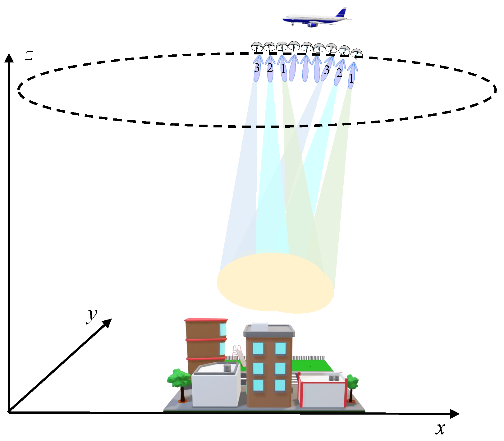
The advantages of CSAR are closely tied to its 360-degree observation capability. However, the limited spotlight region is one of the factors that hamper the development of CSAR. The spotlight region is affected by many factors, such as pulse repetition frequency, beam width, and range ambiguity [14]. In 2014, Ponce et al. [15] conducted theoretical and technical research on Multiple-Input Multiple-Output (MIMO) CSAR, applying MIMO technology to CSAR to achieve high-resolution imaging of large scenes. In 2021, the AIRCAS conducted research on multi-beam CSAR technology to expand the spotlight area of CSAR.

Compared to traditional linear SAR, CSAR offers unparalleled advantages. However, owing to the intricate motion trajectory of CSAR, traditional imaging algorithms designed for linear trajectories are no longer applicable. Currently, CSAR imaging algorithms can be broadly categorized into two types: time-domain imaging algorithms and frequency-domain imaging algorithms. Time-domain imaging algorithms, such as the cross-correlation algorithm [16], confocal projection algorithm [6,17], and backprojection (BP) algorithm [18,19], find application in CSAR. Notably, the BP algorithm stands out due to its versatility in handling various imaging geometries. Nonetheless, it is crucial to acknowledge that the BP algorithm is hampered by high computational complexity and low efficiency. On the other hand, frequency-domain imaging algorithms achieve focused imaging through Fourier transforms in the frequency domain. Examples include the polar format algorithm (PFA) [20] and the wavefront reconstruction algorithm proposed by Soumekh [5]. Nevertheless, these algorithms encounter challenges associated with their limited adaptability to diverse scenes and complex implementation processes [21]. Furthermore, the inherent approximation procedures can affect the imaging accuracy of high-resolution CSAR.

For airborne SAR platforms, imaging errors can be introduced due to airflow disturbances and carrier mechanical vibrations [22]. The trajectory of CSAR is intricate, and the synthetic aperture time is prolonged, making the impact of motion errors significant. Unlike traditional linear SAR, CSAR motion compensation does not require aligning with an ideal trajectory. It only needs to correct slant-range errors and phase errors arising from trajectory measurement inaccuracies and other factors [23]. The accuracy of the navigation system plays a crucial role in obtaining high-resolution CSAR images. To achieve superior imaging quality, the trajectory measurement errors need to be controlled within $1/16$ of the wavelength [24]. Additionally, CSAR faces challenges in motion compensation due to the strong coupling between the range and azimuth, along with the complexity of slant-range expressions. These factors contribute to the increased difficulty in motion compensation for CSAR.

In 2011, Lin et al. [25] introduced a CSAR focusing algorithm based on echo generation. This method performs reverse echo generation by extracting the phase error of point targets after coarse imaging to achieve motion compensation. Zhou et al. [22] conducted a detailed analysis in 2013 of the impact of three-dimensional position errors of the radar on the envelope and phase of the echo. In 2015, Zeng et al. [26] proposed a high-resolution SAR autofocus algorithm in polar format to address the challenge of insufficient inertial navigation accuracy for spotlight SAR, thereby achieving high-resolution imaging. In the same year, Zhang et al. [27] presented a CSAR autofocus algorithm based on sub-aperture synthesis to address the issue of diminished imaging resolution resulting from variations in target scattering coefficients with observation angles. In 2016, Luo et al. [28] introduced an extended factor geometric autofocus algorithm for time-domain CSAR. This innovative approach combines factorized geometrical autofocus (FGA) with fast factorized backprojection (FFBP) processing, relying on gradually changing trajectory parameters to obtain a clear image. In 2017, Wang et al. [29] introduced a sub-bandwidth phase-gradient autofocus method to accomplish motion compensation for high resolution. In 2018, Kan et al. [30] quantitatively analyzed the peak-drop coefficient of the target in the presence of motion errors and assessed the impact of motion errors on imaging quality based on the peak-drop coefficient. In 2023, Li et al. [31] proposed an autofocus method based on the Prewitt operator and particle swarm optimization (PSO). This method aims to enhance imaging quality by optimizing the autofocus process using the Prewitt operator and the PSO algorithm. In general, current motion compensation methods for CSAR can be broadly categorized into two types: one that relies on a high-precision Position and Orientation System (POS), and another based on echo data. However, relying on the motion compensation of a POS is generally challenging, as it is difficult to meet the accuracy requirements of high-resolution CSAR [24,32,33]. On the other hand, motion compensation based on echo data involves estimating the motion-induced errors in the echo signal, which can be a complex process and is susceptible to interference from clutter signals [7]. The long synthetic aperture in CSAR introduces more complex motion errors compared to linear SAR, making it difficult to directly apply classical autofocus algorithms to CSAR [22]. Therefore, specialized motion correction algorithms are needed to address the unique challenges of CSAR.

Currently, motion compensation in CSAR primarily investigates the impact of radar positioning errors on imaging, with a notable scarcity of research on compensating for motion errors using acceleration data. In fact, the degree of deformation experienced by the arm connected to the Inertial Measurement Unit (IMU) and the Global Positioning System (GPS) is proportional to the acceleration. Errors caused by deformation can be determined by analyzing the acceleration information. The innovation of this paper is to analyze the relationship between the acceleration information of the airborne platform and the motion error and propose a high-resolution CSAR motion compensation technology based on the platform’s acceleration information. After calibrating system parameters, it uses acceleration data to directly calculate the amount of motion error caused by deformation. In contrast to the traditional method, there is no need to employ point targets for calibrating the phase error of each scene. Point targets only need to be introduced after calibrating the system’s deformation error parameters. Then, the phase errors of different scenes or different sub-apertures can be directly calculated according to the acceleration. This method reveals the existence of a correlation between the acceleration and residual phase errors and reduces the need for point targets. Finally, the effectiveness of this method is verified through airborne flight experiments. The results demonstrate that the algorithm significantly improves the peak sidelobe ratio (PSLR) and integral sidelobe ratio (ISLR) of the target, thereby achieving high-quality imaging for CSAR.

This article is structured as follows. Section 2 introduces the signal model of multi-beam CSAR and the motion error analysis of CSAR. In Section 3, a high-resolution CSAR motion compensation algorithm is proposed, utilizing the acceleration information of the carrier platform. In Section 4, we introduce the airborne flight experiments and data acquisition. The proposed algorithm is validated through simulation and experimental data in Section 5. These results are further discussed and analyzed in Section 6, where the relationship between the acceleration information and residual phase error is explored. Conclusions are given in Section 7.

2. Theory

This section introduces the signal reconstruction model of airborne multi-beam CSAR and the motion error analysis of CSAR.

2.1. Azimuth Signal Reconstruction Model

The azimuth beam width is one of the factors that restrict the spotlight region of CSAR. Multi-beam CSAR essentially extends the concept of azimuth multi-channel SAR. This is achieved by configuring a beam directed toward different azimuthal directions, effectively expanding the observation area of CSAR. The observation geometry of multi-beam CSAR is depicted in Figure 1, whereas Figure 2 illustrates the observation geometry of CSAR. The SAR platform flies around a circle, and the radar points to a specific angle within each pulse repetition time (PRT), with N PRTs being scanned repeatedly in a group. The data collected at the same angle are considered as an azimuth channel, resulting in N channels of data. The pulse repetition frequency (PRF) of each channel is $1/N$ of the system’s PRF. The multi-channel data essentially utilize the same set of transmitting and receiving antennas, with each channel pointing to different positions at different times. The amplitude and phase errors between the multi-channel data are small and can be considered negligible. This paper primarily focuses on the motion error analysis of CSAR.

In this context, the flight direction of the carrier is referred to as the azimuth direction, whereas the radar line-of-sight direction corresponds to the range direction. The positive direction of the X-axis represents the relative starting point, and the azimuth angle is denoted as $\theta$. The radar transmits a chirp signal, with the carrier frequency denoted as $f_c$, pulse width denoted as $T_p$, and frequency modulation denoted as $K_r$. The expression for the chirp signal is as follows:

$$s_r(t)=rect(\frac{t}{T_p})exp\left\{j\pi K_r{t}^2\right\}$$

(1)

Assuming channel $n_c$ as the reference channel and considering a side-looking antenna configuration, the echo signal from a single point target located at P can be expressed as follows:

$$\begin{array}{cc}\hfill s_0(\tau ,\eta )=& A_0{w}_r(\tau -\frac{2R_p(\eta )}{c})\hfill \\ \hfill & ·exp\left\{j\pi K_r{(\tau -\frac{2R_p(\eta )}{c})}^2\right\}·exp\left\{-j\frac{4\pi R_p(\eta )}{\lambda }\right\}\hfill \end{array}$$

(2)

where $A_0$ is the backscattering coefficient of the target P, $\tau$ is the range fast time, $\eta$ is the azimuth slow time, $w_r(·)$ is the range gate function, $\lambda$ is the working wavelength of the radar, and $R_p(\eta )$ is the distance between the radar and the target P at the azimuth time $\eta$. The signal after pulse compression can be expressed as

$$\begin{array}{cc}\hfill s_{rc}(\tau ,\eta )=& A_{0}sin\mathrm{c}(K_r{T}_p(\tau -\frac{2R_p(\eta )}{c}))\hfill \\ \hfill & ·exp\left\{-j\frac{4\pi R_p(\eta )}{\lambda }\right\}\hfill \end{array}$$

(3)

After pulse compression, the data are subjected to Fourier transform in the azimuth direction to obtain $S_{n_c}(\tau ,f_a)$, where $f_a\in [-prf/2,prf/2]$, $prf=PRF/N$. The time interval between the adjacent channels of the multi-channel data is expressed as $\Delta \delta =1/(N·prf)$. In the case of the azimuth multi-channel data, each channel has a different beam center pointing angle. When the pulse repetition frequency is small, there can be Doppler ambiguity. The multi-channel data are initially deblurred and then interpolated to match the original data length, resulting in the deblurred signal $S_n(\tau ,f)$, where $f\in [-prf·N/2,prf·N/2]$. Subsequently, the reconstructed pulse compression data can be obtained by compensating for the delay factor, with $n_c$ serving as the reference channel.

$$\stackrel{⌢}{S}(\tau ,f)=\sum _{n=1}^N{S}_n(\tau ,f)·exp\left\{j2\pi f·(n-n_c)\Delta \delta \right\}$$

(4)

2.2. Motion Error Analysis of CSAR

This paper employs the BP algorithm for conducting two-dimensional imaging in CSAR. The BP algorithm, being a time-domain imaging algorithm, is not limited by the flight trajectory. It possesses qualities such as high imaging accuracy, broad applicability, and straightforward implementation, making it one of the primary imaging algorithms for CSAR [34]. During CSAR imaging processing, it is crucial to select an appropriate reference plane as the focusing plane. The correct reference height enables target focusing, whereas an incorrect reference height results in the target defocusing into a circle [9,35].

The plane with height $z_{ref}$ is selected as the reference plane, and the reference plane is divided into uniform grids to obtain the imaging grid $N_x\times N_y$. $\stackrel{⌢}{s}(\tau ,\eta )$, the time-domain signal after pulse compression, is obtained through an inverse Fourier transform of Equation (4). To determine the point $P(x,y,z_{ref})$ on the grid, we calculate the time delay $\Delta t_p$ from the radar to the point at the azimuth time $\eta$. Subsequently, we employ interpolation within the signal $\stackrel{⌢}{s}(\tau ,\eta )$ to locate the echo data that correspond to the calculated time delay $\Delta t_p$. This interpolation operation enables us to retrieve the desired echo information for point P on the grid. After that, the interpolated data need to be compensated for the phase factor $exp(j4\pi R_{\mathrm{zref}}(\eta )/\phantom{R_{\mathrm{zref}}(\eta )\lambda }\lambda )$, where $R_{zref}(\eta )$ is the distance from the radar at the azimuth time $\eta$ to the reference plane. The phase factor $exp(j4\pi R_{\mathrm{zref}}(\eta )/\phantom{R_{\mathrm{zref}}(\eta )\lambda }\lambda )$ is related to the reference plane. Finally, the echo data obtained at all azimuth moments of the grid $(x,y,z_{ref})$ are coherently superimposed to obtain a two-dimensional image, as shown in Equation (5).

$$\mathrm{I}(x,y,z_{ref})=\sum _{\eta }\stackrel{⌢}{s}(\tau ,\eta )·exp(j4\pi R_{zref}(\eta )/\phantom{R_{zref}(\eta )\lambda }\lambda )$$

(5)

When the airborne platform is flying in a circular trajectory, it is susceptible to external factors that can introduce deviations between the radar measurement coordinates obtained from the navigation system and the actual coordinates. As shown in Figure 3, the radar position information obtained from the navigation system is A, and the actual radar position information is $A^{\prime }$. For the point target P in the scene, its motion error can be expressed as the slant-range variation. At the azimuth time $\eta$, the slant distance from the actual radar coordinate to the target can be expressed as

$${\stackrel{⌢}{R}}_p(\eta )=R_p(\eta )+\Delta R_p(\eta )$$

(6)

Here, $R_p(\eta )$ is the measured slant distance, and $\Delta R_p(\eta )$ is the change in the slant distance caused by the motion error. Without considering the azimuth signal reconstruction, the echo after pulse compression can be expressed as

$$\begin{array}{cc}\hfill s_{\stackrel{⌢}{rc}}(\tau ,\eta )=& A_{0}sin\mathrm{c}(K_r{T}_p(\tau -\frac{2{\stackrel{⌢}{R}}_p(\eta )}{c}))\hfill \\ \hfill & ·exp\left\{-j\frac{4\pi {\stackrel{⌢}{R}}_p(\eta )}{\lambda }\right\}\hfill \end{array}$$

(7)

Measurement errors between the actual trajectory and the measured trajectory are inevitable due to atmospheric disturbances and other factors. These errors introduce phase errors in the echo signal, preventing the coherent accumulation of energy and resulting in unfocused images. The phase error caused by residual motion errors in the cross-range resolution unit is the primary factor leading to image defocusing [24].

The multi-beam CSAR extends the spotlight region of CSAR through scanning. The BP algorithm is used to image the signal after azimuth reconstruction, providing robust imaging capabilities. However, the traditional BP algorithm is a time-domain imaging algorithm, lacking a clear Fourier transform relationship in the processed signal. As a result, the conventional autofocus methods cannot be directly applied to the BP imaging algorithm [36]. Moreover, the flight trajectory of CSAR is complex, and the aircraft attitude changes frequently. The non-rigid connection between the IMU and GPS introduces significant errors in the POS’s solution process. The inaccurate POS position information and complex beam pointing contribute to phase errors in the reconstructed signal, making compensation challenging. In light of these issues, this study focuses on motion compensation technology for high-resolution CSAR and leverages acceleration information from the POS to achieve high-resolution imaging in CSAR.

3. Method

This paper conducts two-dimensional imaging of multi-beam CSAR data and proposes a motion compensation algorithm for CSAR based on acceleration information from the airborne platform. The algorithm utilizes radial acceleration data from the POS to address phase errors stemming from deformation. Initially, azimuth reconstruction and coarse imaging of multi-beam CSAR data are undertaken. Following this, the ground calibrators within the image are chosen to extract deformation errors. Acceleration is employed for estimating and calibrating the system’s deformation error parameters. Ultimately, leveraging the calibrated system parameters, the deformation error of the imaging scene can be computed based on acceleration, facilitating subsequent phase compensation. The proposed method in this paper is categorized into two main parts: data preprocessing and phase error compensation based on acceleration information. The primary processing flow is outlined as follows:

• The raw echo data undergo range-pulse compression, and the resulting data post-pulse compression are extracted at $1/N$ intervals to obtain multi-channel data.
• The data are converted into the azimuth frequency domain, and the Doppler center frequency is estimated. Subsequently, the data undergo interpolation and de-ambiguity processing.
• Compensating for the delay factor in multi-channel data achieves time-domain alignment, followed by the reconstruction of the multi-channel signal with reference to the content in Section 2.1.
• The BP algorithm is employed for two-dimensional imaging. Calibrators are selected to mark the deformation error $\epsilon (\theta )$ in the two-dimensional frequency domain.
• Acceleration information is calculated from the POS, the phase error $\epsilon (\theta )$ is linearly estimated from the acceleration, and the system deformation error coefficient K is calibrated.
• Using the system parameter K calibrated in the previous step, the phase error requiring compensation based on acceleration is calculated, and error compensation in the frequency domain is performed to obtain the focused image after compensation.

The overall flowchart is illustrated in Figure 4.

The complete algorithm for data preprocessing is given in Algorithm 1.

Algorithm 1 Multi-beam CSAR data preprocessing.

Input: Radar raw echo Initialization: The raw echo is processed using pulse compression. Define the beam center pointing angle, radar system $PRF$, azimuth channel number N, and reference channel $n_c$.      Step 1: The multi-beam CSAR data after pulse compression are extracted to obtain N sub-channel data;      Step 2: The autocorrelation method is used to estimate and calculate the Doppler center frequency $f_{dc}$ of each channel;      Step 3: The Doppler ambiguity m is calculated according to the oblique angle of the antenna beam center, and the ambiguity is solved to obtain $f_d=f_{dc}+m·prf$;      Step 4: The multi-channel data are zero-padded in the frequency domain so that the data of each channel are equal to the length of the data before extraction;      Step 5: Multiple sets of data are interpolated to compensate for the phase factor $exp(j2\pi f·(n-n_c)\Delta \delta )$, where $\Delta \delta =1/PRF$;     Step 6: Multi-channel data are accumulated according to Formula (4) to obtain $\stackrel{⌢}{S}(\tau ,f)$; % Accumulate multi-channel data $\stackrel{⌢}{S}(\tau ,f)={\displaystyle \sum _{n=1}^N}{S}_n(\tau ,f)·exp(j2\pi f·(n-n_c)\Delta \delta )$;      An azimuth inverse Fourier transform is performed to obtain the reconstructed      time-domain pulse-pressure data $\stackrel{⌢}{s}(\tau ,\eta )=IFFT\left[\stackrel{⌢}{S}(\tau ,f)\right]$;      Step 7: Time-domain two-dimensional imaging using the BP algorithm. Output: CSAR two-dimensional images.

Assuming that the image with the phase error is represented as $s_{\epsilon }(x,y)$, the spectrum obtained through the two-dimensional FFT is $S_{\epsilon }(k_x,k_y)$.

$$\begin{array}{c}\hfill S_{\epsilon }(k_x,k_y)=\underset{x}{\int }\underset{y}{\int }{g}_{\epsilon }(x,y)exp(-j{k}_{x}x-j{k}_{y}y)dxdy\end{array}$$

(8)

$$\begin{array}{c}\hfill k_x=-\frac{4\pi f}{c}sin\alpha cos\theta \end{array}$$

(9)

$$\begin{array}{c}\hfill k_y=-\frac{4\pi f}{c}sin\alpha sin\theta \end{array}$$

(10)

Assuming the target position is $(x_p,y_p)$, under ideal conditions, the two-dimensional spectral phase only includes the initial phase of the target and the linear phase related to the target position. By neglecting the initial phase and the envelope of the transmitted signal spectrum, we obtain Equation (11).

$$\begin{array}{c}\hfill S_0(k_x,k_y)=exp(-j{k}_x{x}_p-j{k}_y{y}_p)\end{array}$$

(11)

The phase difference between $S_{\epsilon }(k_x,k_y)$ and $S_0(k_x,k_y)$ is the phase error. From Equation (7), it can be observed that the phase error at the central wavenumber primarily influences imaging. Therefore, the residual phase can be expressed as:

$$\begin{array}{c}\hfill \epsilon (\theta )=\frac{4\pi }{\lambda }\Delta R(\theta )\end{array}$$

(12)

The time-domain image obtained through the BP algorithm exhibits periodic blurring in the spectrum when the imaging grid is relatively large, i.e., when it does not satisfy the grid spacing required for full-aperture imaging. Therefore, before establishing the time-frequency relationship between the two-dimensional wavenumber domain $(k_x,k_y)$ and the angular wavenumber domain $(\theta ,K)$, deblurring is necessary. The central frequencies of the two-dimensional spectrum of the radar signal can be expressed as $f_{xc}=f_c·sin\alpha ·cos\theta$ and $f_{yc}=f_c·sin\alpha ·sin\theta$, where $\theta =arctan(\frac{f_y}{f_x})$, $\alpha$ is the look angle of the radar, and $f_c$ is the radar signal carrier frequency. Under full-aperture conditions, the plane resolution of CSAR can be expressed as

$$\begin{array}{c}\hfill \rho \approx \frac{c}{4sin\alpha ·f_{max}}\end{array}$$

(13)

where $f_{max}=f_c+B/\phantom{B2}2$, and B is the signal bandwidth. When the imaging grid spacing is $\Delta x=\Delta y$, the frequency range obtained in the $f_x$ and $f_y$ directions is $\left[-c/(4\Delta x),c/(4\Delta x)\right]$, and the blur period can be represented as

$$\begin{array}{c}\hfill \begin{array}{c}{M}_x=round(f_{xc}/(c/(2\Delta x)))\hfill \\ M_y=round(f_{yc}/(c/(2\Delta y)))\hfill \end{array}\end{array}$$

(14)

where $M_x$ is the blur number in the $f_x$ direction, and $M_y$ is the blur number in the $f_y$ direction. Finally, the residual phase at the central frequency is extracted from the frequency-domain image.

However, there is no direct relationship between the azimuth time and phase error. We need to extract the phase error for each sub-aperture. Sometimes, there is no suitable isolated point target in the scene, and the phase error is difficult to obtain directly. Therefore, a more adaptive method is needed. This article proposes a CSAR motion compensation method based on acceleration information. Radial acceleration can, to some extent, reflect the degree of deformation of the lever arm between the IMU and GPS. Furthermore, radial acceleration can reflect motion errors. In this paper, a motion compensation method for CSAR based on acceleration information is proposed, which uses the acceleration to estimate the phase error of each sub-aperture and then compensates to obtain the focused image. The complete algorithm for CSAR motion compensation based on acceleration information is given in Algorithm 2.

Algorithm 2 CSAR motion compensation algorithm based on acceleration.

Input: Two-dimensional CSAR images. Initialization: Select the calibrator and apply windowing to reduce clutter and interference from nearby targets, obtaining data $s_{\epsilon }(x,y)$.      Step 1: Perform a two-dimensional Fourier transform on $s_{\epsilon }(x,y)$ to move to the frequency domain $S_{\epsilon }(k_x,k_y)$;      Step 2: Deblur in the frequency domain. $M_x=round(f_{xc}/(c/(2\Delta x)))$, $M_y=round(f_{yc}/(c/(2\Delta y)))$;      Step 3: Extract the phase at the central wavenumber $k_c$ and unwrap the phase;      Step 4: Remove the linear phase to extract the residual phase errors $\epsilon (\theta )$; obtain the residual motion errors $\Delta R(\theta )$ based on Equation (12);      Step 5: Calculate the radial acceleration $ar(\theta )$ using POS data;      Step 6: The radial acceleration information $ar(\theta )$ and motion error $\Delta R(\theta )$ are estimated using the least-square method; determine the system parameter K;      Step 7: According to the system parameter K obtained in Step 6, the phase error is calculated and compensated through the acceleration, and the compensated spectrum $S(k_x,k_y)$ is obtained;      Step 8: Perform a two-dimensional inverse Fourier transform on $S(k_x,k_y)$ to obtain the motion-compensated image $s(x,y)$;      Step 9: For the new scene, after transforming to the two-dimensional frequency domain, Steps 7 and 8 are repeated to obtain the compensated focusing image. Output: Two-dimensional CSAR image after motion compensation.

4. Airborne Experiments and Data Acquisition

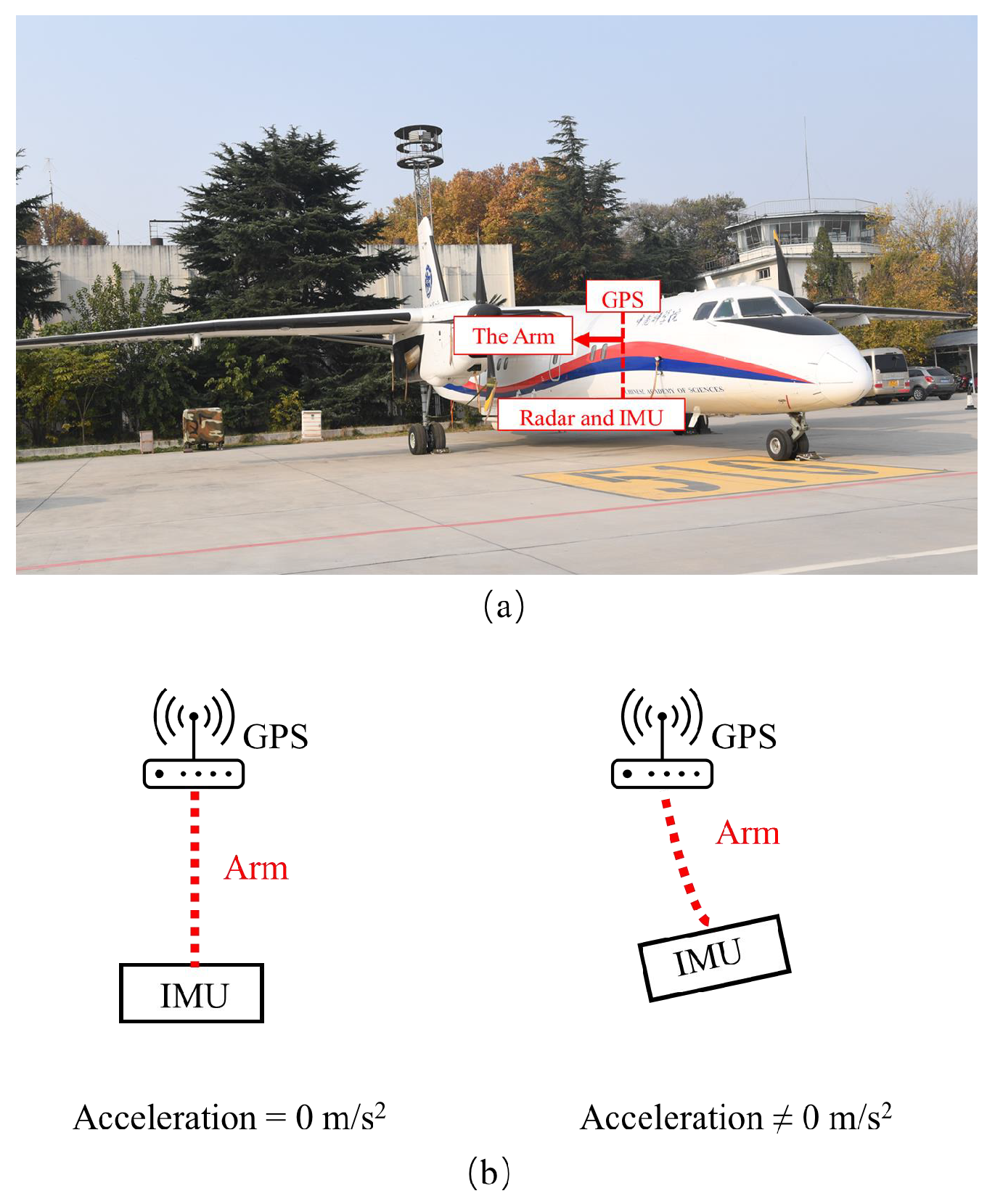
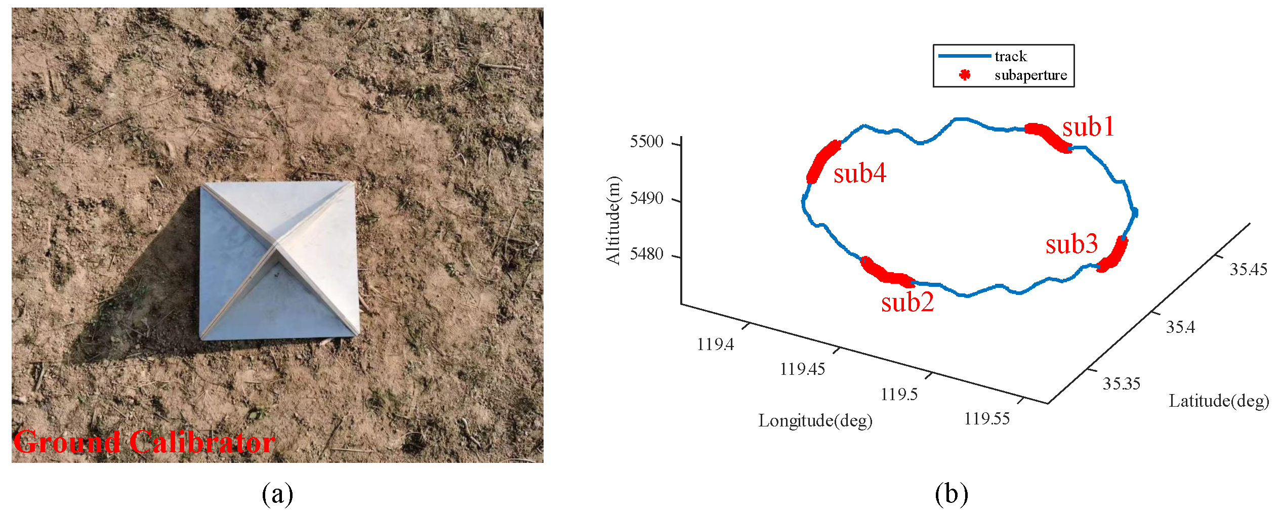
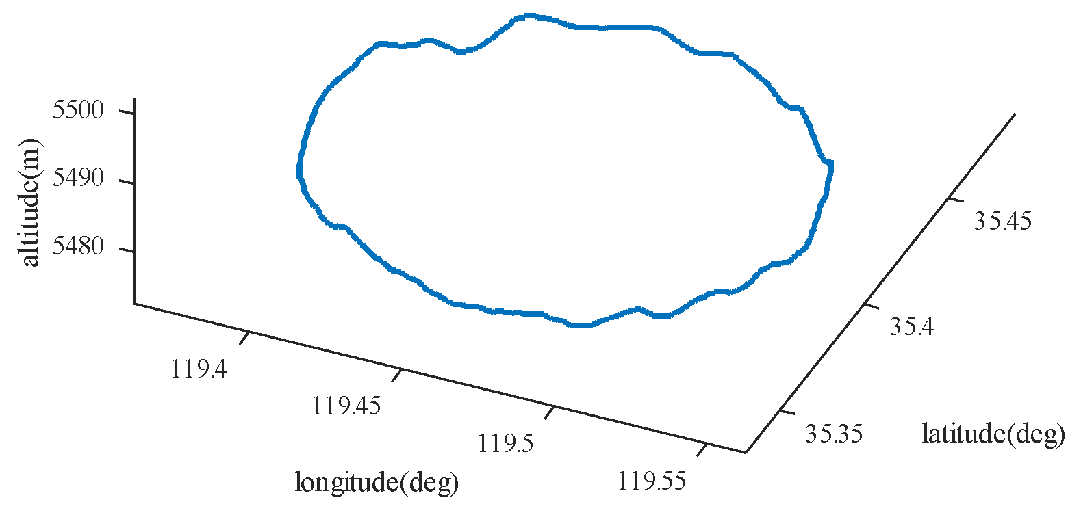
In 2021, AIRCAS conducted airborne multi-beam CSAR flight experiments in Rizhao, Shandong, China. The experimental system is shown in Figure 5. The GPS antenna is located on top of the aircraft, and the phased-array radar closely integrated with the IMU is positioned on the belly of the aircraft. The system is configured with six beam positions, scanning from $-10$ deg to $+10$ deg. The aircraft flies counterclockwise at an altitude of 5500 m, with the radar operating in the left-looking mode and the working frequency band in the X-band.

Table 1. Multi-beam CSAR system parameters.

Parameter	Symbol	Value
Bandwidth	$B_w$	1200 MHz
Flight height	H	5500 m
Azimuth sampling rate	$F_a$	5000 Hz
Wave band	\	8∼12 GHz (X-band)
Polarization	\	HH

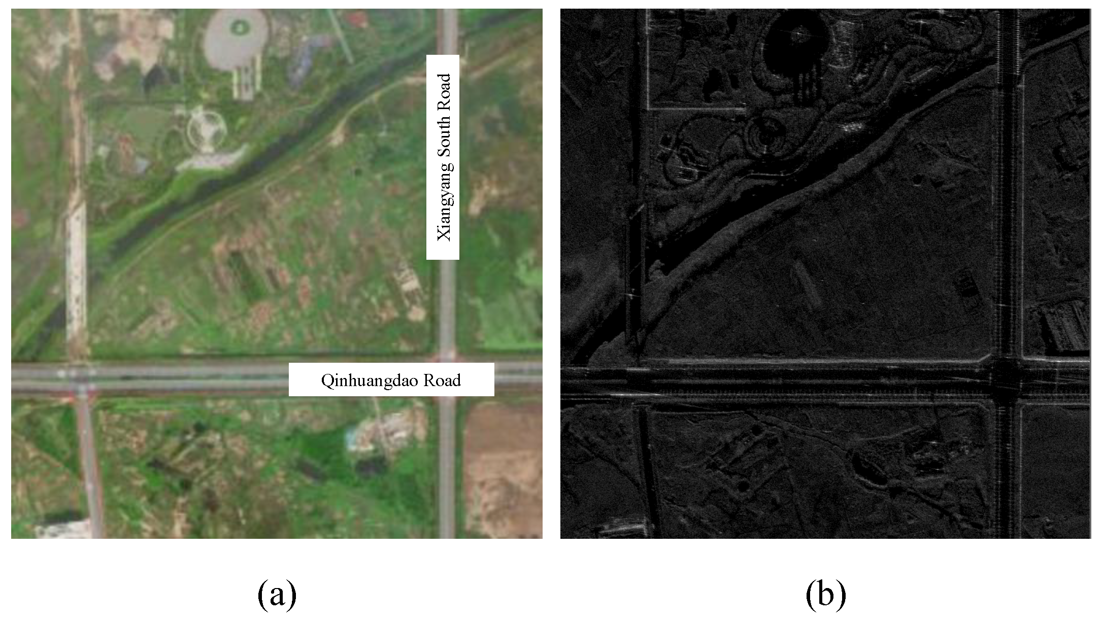
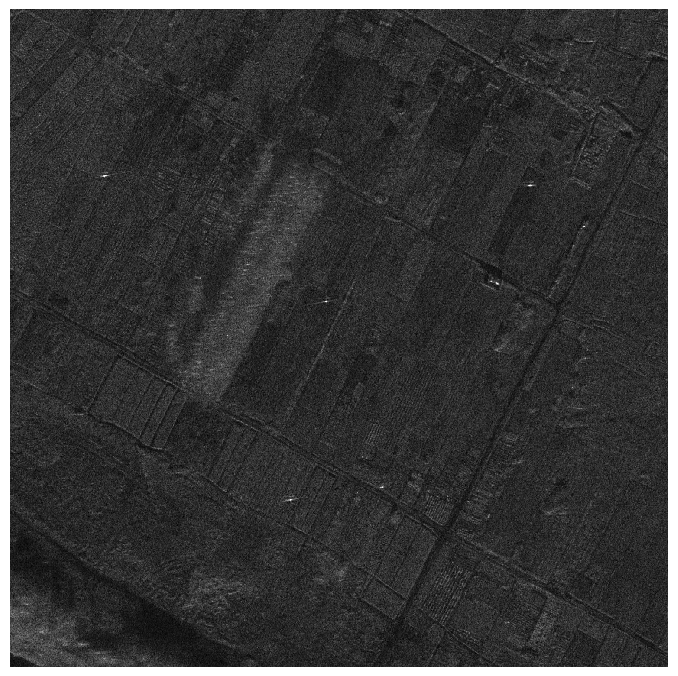
provides the configuration parameters of the airborne multi-beam CSAR experimental system. Figure 6 illustrates the flight trajectory of the radar platform. Figure 7 shows an optical image and a SAR image of the imaging area.

Before imaging, it is necessary to reconstruct the azimuth signal of the obtained multi-beam CSAR. This involves deinterleaving the data after pulse compression to extract multi-beam data, numbering channel 1 to channel 6, respectively. To estimate the center frequency of the signal in the baseband, the autocorrelation method is employed. Additionally, the Doppler ambiguity is resolved by considering the beam-pointing relationship. The multi-channel data are then deblurred and interpolated in the frequency domain, ensuring that the data length matches that of the original data and compensating for the delay phase factor. Subsequently, the multi-channel data are combined into a single-channel signal, with attention given to the energy balance during spectrum splicing. As shown in Figure 8, four sub-apertures with varying angles are chosen for data preprocessing, leading to the generation of reconstructed signals and imaging results. The sub-aperture length is set to 6000 pulses. The reconstructed data can be imaged, but they still have the residual phase error. Therefore, it is necessary to study CSAR motion compensation technology based on acceleration information.

5. Experimental Results

The proposed method’s effectiveness is initially validated through simulation experiments. The verification process involves introducing a known error into the simulation data and utilizing the proposed method for estimation and compensation. It is noteworthy that the introduced error should be associated with acceleration information. The method proposed in this paper primarily focuses on compensating for the system error arising from the deformation of the lever arm due to rapid changes in platform acceleration. In actual data processing, we chose a calibration field for the purpose of validity verification. The process involves coarse imaging of a sub-aperture, followed by deformation phase error extraction and system parameter calibration to establish the relationship between the acceleration and phase error. Subsequently, the acceleration is utilized to directly estimate and compensate for the motion errors of the remaining sub-apertures. An analysis of the results before and after compensation is conducted to validate the efficacy of the proposed method.

5.1. Simulation Experiments

This section employs real POS data and incorporates system parameter design to conduct semi-physical simulation experiments. The synthetic aperture size is set to 10 deg. Referring to the actual radial acceleration information, a slant-range error is added, as shown in Figure 9, with an error greater than $\lambda /16$.

Table 2. Coordinates of the scene center and point targets.

	Position Coordinate (m)		Position Coordinate (m)
Scene center	(−320, −120.0)	C	(−315, −135.0)
A	(−320, −120.0)	D	(−325, −125.0)
B	(−315, −125.0)	E	(−325, −135.0)

provides the coordinates of the scene center and point targets. The imaging grid size is $400\times 400$.

To verify the effectiveness of the algorithm, the method proposed in this paper was compared with that in [25], as shown in Figure 10 and

Table 3. Simulation data, characteristic analysis of the target in the azimuth direction.

Point Number	Method 1 1			Method 2 2
	IRW (m)	PSLR (dB)	ISLR (dB)	IRW (m)	PSLR (dB)	ISLR (dB)
A	$0.098$	$-13.31$	$-10.630$	$0.097$	$-13.30$	$-10.642$
B	$0.098$	$-13.31$	$-10.625$	$0.097$	$-13.31$	$-10.644$
C	$0.098$	$-13.32$	$-10.625$	$0.098$	$-13.32$	$-10.644$
D	$0.098$	$-13.30$	$-10.624$	$0.097$	$-13.30$	$-10.645$
E	$0.098$	$-13.31$	$-10.621$	$0.098$	$-13.31$	$-10.641$
Imaging time	88.7 s			1.6 s
Point targets	Each azimuth time error			Point targets are only required
	extraction requires point targets.			when determining system parameters.

¹ The comparison method [25]. ² The proposed method.

. It can be seen that both methods can achieve good focusing effects. However, the algorithm proposed in this article has lower time complexity and less dependence on point targets. The proposed method calculates the deformation error based on the acceleration in the wavenumber domain, with a time complexity of $\mathrm{O}(N^{2}logN)$. Furthermore, in contrast to traditional methods, which involve coarse imaging and error calculation for each sub-aperture, the proposed approach requires the use of point targets only in the initial sub-aperture to establish the system parameters between the deformation error and acceleration. Subsequently, it can calculate and compensate for the phase errors of the remaining sub-apertures based on acceleration. The system parameters are equally applicable to different scenes, so deformation error compensation can be performed even if there are no suitable point targets in the new scene. This not only saves time in extracting each sub-aperture error but also reduces dependence on point targets.

It is noteworthy that, to some extent, acceleration reflects the degree of deformation between the IMU and GPS, so analyzing the relationship between the acceleration and residual phase error is meaningful. Due to the relatively complex flight trajectory of CSAR, the direction of the aircraft’s velocity and acceleration constantly changes, and the non-rigid connection between the GPS and IMU introduces significant errors in the radar position solution of the POS. Therefore, referencing the radar’s three-dimensional position coordinates for imaging introduces residual phase errors. This paper creatively introduces acceleration information and utilizes it for residual phase error estimation. Following parameter calibration, the phase error caused by deformation can be estimated and compensated through acceleration.

5.2. Real Data Experiments

This section validates the effectiveness of the proposed method using real data. The characteristics of the ground calibrators are analyzed. The ground calibrators used in the experiment are assembled using four triangular reflectors, as shown in Figure 11. Based on the opening directions of the ground calibrators, four sub-apertures are selected in this paper, each with an aperture length of 96,000 pulses. One sub-aperture is used for parameter estimation, and the other three sub-apertures are used to verify the effectiveness of the proposed method. The method in this article needs to determine the parameter relationship between the acceleration and phase error through sub-aperture sub1. It is worth noting that during the parameter determination stage, point targets need to be calibrated. Afterward, both the errors of the other sub-apertures and the errors of other new scenes can be calculated and compensated through acceleration, and point targets are no longer needed.

Taking the north direction as an example, the aperture sub1 is used for two-dimensional imaging and parameter estimation. As depicted in Figure 12a, one group of ground calibrators is windowed to suppress the influence of surrounding clutter, and the image $s_{\epsilon }(x,y)$ is obtained. A two-dimensional Fourier transform is performed to obtain the frequency-domain image $S_{\epsilon }(k_x,k_y)$. To facilitate subsequent phase extraction, the spectral phase variation should not be too dense. Here, we employ cyclic shifting to position the target point at a corner of the image. This approach effectively reduces errors in phase unwrapping.

According to Section 3, we know that for the spectrum phase, we only need to calculate the residual phase at the center of the spectrum, that is, the phase at position $(f_{xc}(\theta ),f_{yc}(\theta ))$. As shown in Figure 13, the phase at the center frequency is extracted, and phase unwrapping is performed. Then, the linear phase is removed, as shown in Figure 13b, representing the phase errors that need compensation. According to Equation (12), $\Delta R(\theta )$ can be calculated for motion compensation.

Figure 14a shows the speed of the carrier in the POS in three directions and derives it to obtain the acceleration in those directions. Figure 14b shows the radial acceleration after coordinate system transformation, and it can be seen that the change in the trend of the radial acceleration is consistent with the change in the trend of the phase error. The phase error is estimated using acceleration information through a least-squares method, and the estimated results are shown in Figure 15.

Phase compensation is applied to the scene, and the results are shown in Figure 16. Figure 17 provides information on the calibrator, showing the results of residual phase compensation based on acceleration. The target is effectively compensated, and the experimental results verify the effectiveness of phase error estimation based on acceleration.

The parameter relationship between the acceleration information and motion errors has been established through least-squares estimation. Now, for different sub-apertures, radial acceleration can be calculated from the POS. This parameter is then used for phase error estimation, resulting in the estimation results for phase compensation. Figure 18 shows the extracted phase error and acceleration estimation results for the other three sub-apertures. These results validate the feasibility of the proposed method, and the system parameters estimated through sub-aperture sub1 can be effectively applied to sub-apertures sub2, sub3, and sub4.

Figure 19 shows the spectral phase results of the point target before and after three different sub-aperture motion error compensations. The target characteristics from Figure 17 and Figure 19 are analyzed and the results are presented in

Table 4. Actual data, characteristic analysis of the target in the azimuth direction.

Point Number	Original Image			This Work
	IRW (m)	PSLR (dB)	ISLR (dB)	IRW (m)	PSLR (dB)	ISLR (dB)
1	$0.067$	$-2.88$	$1.71$	$0.067$	$-7.08$	$-5.80$
2	$0.130$	$-1.57$	$4.20$	$0.062$	$-7.36$	$-6.39$
3	$0.069$	$-3.28$	$0.45$	$0.066$	$-7.80$	$-4.93$
4	$0.057$	$-4.11$	$-0.56$	$0.058$	$-7.92$	$-6.21$

. The effectiveness of the method has been verified with real data.

6. Discussion

The deformation error of the lever arm exhibits a strong correlation with acceleration. Consequently, this paper introduces a CSAR motion compensation method based on acceleration information. The method initially utilizes point targets to calibrate the system parameters, subsequently calculating the deformation error that requires compensation at each position based on the calibrated parameters and acceleration. Once the system parameters are calibrated, there is no longer a need to employ a point target to estimate the phase error for new scenes and new sub-apertures. This effectively eliminates the dependence on point targets. The method proposed in this paper has been validated through airborne flight experiments, and the experimental results are presented in Section 5.

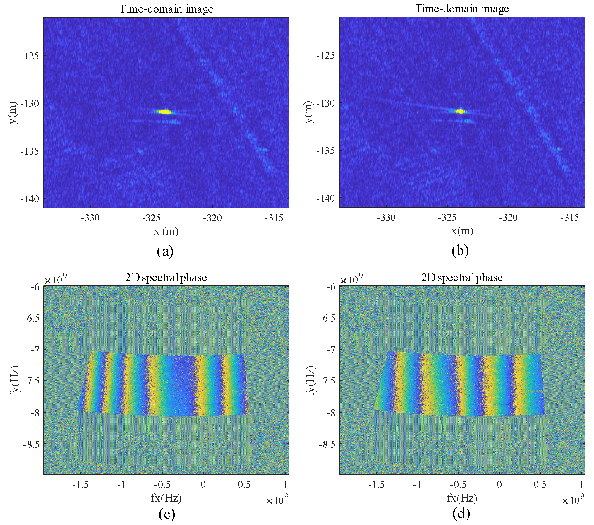
Firstly, we reconstruct the azimuth signal of multi-beam CSAR based on Algorithm 1. Subsequently, motion compensation based on the acceleration information is executed, following the steps outlined in Algorithm 2. As depicted in Figure 12, the selected calibrator (or isolated strong point) is windowed in the image domain, and the synthetic aperture size is set to 15∼20 deg. 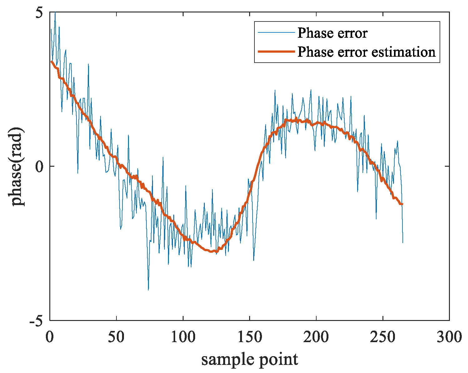Equation (14) is employed for deblurring, resulting in a frequency spectrum phase, as illustrated in Figure 12d. For a target, its frequency spectrum phase should only contain an initial phase and a linear phase, with the phase uniformly varying. We extract the phase at the center frequency, and after unwrapping the phase and removing the linear phase, we obtain a residual phase error. This phase error is challenging to express directly in an equation for compensation during the CSAR imaging process. There is a correlation between the phase error and radial acceleration. 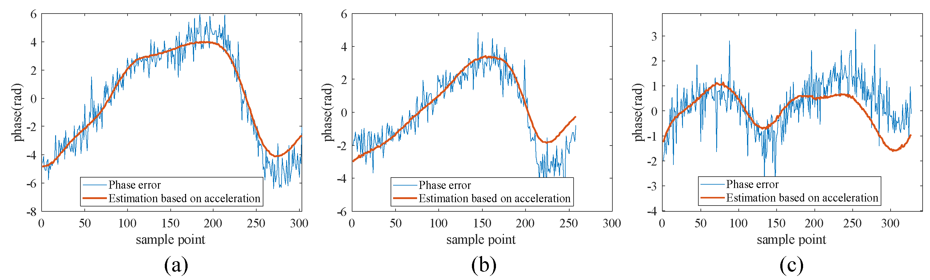The parameter relationship between the acceleration information and phase error can be estimated from a sub-aperture, as shown in Figure 15. This allows us to calculate the phase error compensation required at various azimuth times based on the acceleration information. One source of error is the frequent changes in the flight attitude of CSAR. Coupled with the non-rigid connection between the IMU and GPS, the deformation error of the lever arm becomes significant. The variations in acceleration serve as an indicator of the degree of lever arm deformation. Consequently, utilizing acceleration to estimate residual motion errors is a rational and effective approach. Figure 18 illustrates the estimated results for sub-apertures in various directions. It is evident that the radial acceleration information aligns well with the residual motion error. 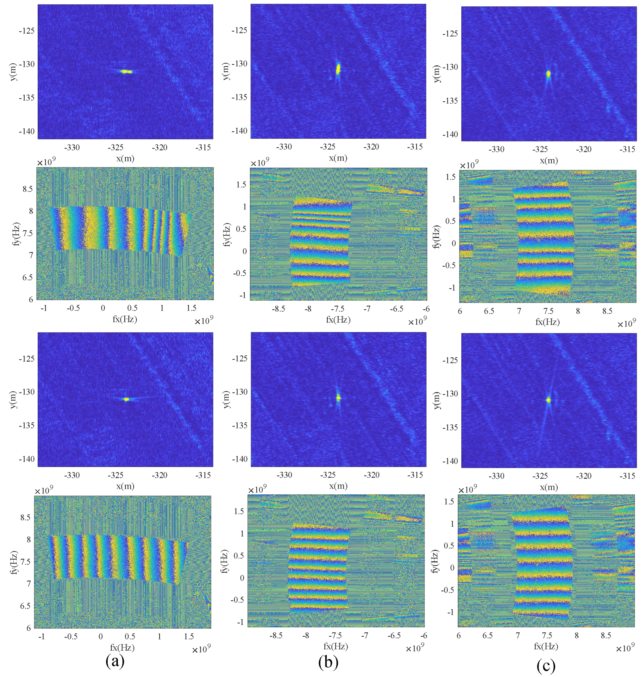Figure 17 and Figure 19 showcase the motion compensation results for four directions. The compensated target’s spectral phase becomes uniform, retaining only the linear phase associated with the target position, resulting in a focused target point. Further analysis of the target’s azimuth characteristics reveals a significant improvement in the peak sidelobe ratio and integral sidelobe ratio, confirming the effectiveness of the proposed method. It is noteworthy that this paper introduces acceleration information creatively and verifies its application in high-resolution CSAR imaging.

7. Conclusions

Considering the complex trajectory of CSAR and the non-rigid connection between the IMU and GPS, the deformation error can cause defocusing in CSAR imaging. Based on the results of airborne flight experiments, this paper determines the correlation between the deformation error and acceleration information and proposes a high-resolution CSAR motion compensation method based on acceleration information. Initially, the parameters for the deformation error are calibrated using a sub-aperture. Subsequently, the deformation error of new scenes or new sub-apertures is computed through acceleration, followed by phase compensation. It is noteworthy that this method requires the use of point targets solely for parameter calibration in the initial sub-aperture. Afterward, both other sub-apertures and new scenes no longer require point targets, thereby reducing dependence on them. After compensation, both the peak sidelobe ratio and integral sidelobe ratio of the target are effectively improved, resulting in enhanced image quality. The effectiveness of the proposed method is validated using airborne measured data. Compared to traditional compensation methods, the introduction of acceleration information provides new insights into the focusing processing of high-resolution CSAR, thereby contributing to the advancement of high-resolution SAR imaging.

References

1. Liu, W.; Sun, G.C.; Xia, X.G.; Fu, J.; Xing, M.; Bao, Z. Focusing Challenges of Ships With Oscillatory Motions and Long Coherent Processing Interval. IEEE Trans. Geosci. Remote Sens. 2021, 59, 6562–6572. [Google Scholar] [CrossRef]
2. Yang, L.; Zhang, F.; Sun, Y.; Chen, L.; Li, Z.; Wang, D. Motion Error Estimation and Compensation of Airborne Array Flexible SAR Based on Multi-Channel Interferometric Phase. Remote Sens. 2023, 15, 680. [Google Scholar] [CrossRef]
3. Liu, W.; Sun, G.C.; Xing, M.; Pascazio, V.; Chen, Q.; Bao, Z. 2-D Beam Steering Method for Squinted High-Orbit SAR Imaging. IEEE Trans. Geosci. Remote Sens. 2021, 59, 4827–4840. [Google Scholar] [CrossRef]
4. Tsz-King, C.; Kuga, Y.; Ishimaru, A. Experimental studies on circular SAR imaging in clutter using angular correlation function technique. IEEE Trans. Geosci. Remote Sens. 1999, 37, 2192–2197. [Google Scholar] [CrossRef]
5. Soumekh, M. Reconnaissance with slant plane circular SAR imaging. IEEE Trans. Image Process. 1996, 5, 1252–1265. [Google Scholar] [CrossRef]
6. Ishimaru, A.; Tsz-King, C.; Kuga, Y. An imaging technique using confocal circular synthetic aperture radar. IEEE Trans. Geosci. Remote Sens. 1998, 36, 1524–1530. [Google Scholar] [CrossRef]
7. Jianfeng, Z.; Yaowen, F.; Wenpeng, Z.; Wei, Y.; Tao, L. Review of CSAR imaging techniques. Syst. Eng. Electron. 2020, 42, 2716–2734. [Google Scholar]
8. Bao, Q.; Lin, Y.; Hong, W.; Shen, W.; Zhao, Y.; Peng, X. Holographic SAR Tomography Image Reconstruction by Combination of Adaptive Imaging and Sparse Bayesian Inference. IEEE Geosci. Remote Sens. Lett. 2017, 14, 1248–1252. [Google Scholar] [CrossRef]
9. Li, Z.; Zhang, F.; Wan, Y.; Chen, L.; Wang, D.; Yang, L. Airborne Circular Flight Array SAR 3-D Imaging Algorithm of Buildings Based on Layered Phase Compensation in the Wavenumber Domain. IIEEE Trans. Geosci. Remote Sens. 2023, 61, 5213512. [Google Scholar] [CrossRef]
10. Ponce, O.; Prats, P.; Scheiber, R.; Reigber, A.; Moreira, A. Analysis and optimization of multi-circular SAR for fully polarimetric holographic tomography over forested areas. In Proceedings of the 2013 IEEE International Geoscience and Remote Sensing Symposium—IGARSS, Melbourne, Australia, 21–26 July 2013; pp. 2365–2368. [Google Scholar]
11. Wang, J.; Lin, Y.; Guo, Z.; Guo, S.; Hong, W. Circular SAR optimization imaging method of buildings. J. Radars 2015, 4, 698–707. [Google Scholar]
12. Lin, Y.; Zhang, L.; Wei, L.; Zhang, H.; Feng, S.; Wang, Y.; Hong, W. Research on Full-aspect Three-dimensional SAR Imaging Method for Complex Structural Facilities without Prior Model. J. Radars 2022, 11, 909–919. [Google Scholar]
13. Hong, W.; Wang, Y.; Lin, Y.; Tan, W.; Wu, Y. Research progress on three-dimensional SAR imaging techniques. J. Radars 2018, 7, 633–654. [Google Scholar]
14. Ponce, O.; Rommel, T.; Younis, M.; Prats, P.; Moreira, A. Multiple-input multiple-output circular SAR. In Proceedings of the 2014 15th International Radar Symposium (IRS), Gdańsk, Poland, 16–18 June 2014; pp. 1–5. [Google Scholar]
15. Ponce, O.; Almeida, F.Q.D.; Rommel, T. Multiple-Input Multiple-Output Circular SAR for High Altitude Pseudo-Satellites. In Proceedings of the Space Generation Congress/International Astronautical Congress Proceedings, Guadalajara, Mexico, 26–30 September 2016. [Google Scholar]
16. Bryant, M.L.; Gostin, L.L.; Soumekh, M. 3-D E-CSAR imaging of a T-72 tank and synthesis of its SAR reconstructions. IEEE Trans. Aerosp. Electron. Syst. 2003, 39, 211–227. [Google Scholar] [CrossRef]
17. Wu, X.; Wang, Y.; Wu, Y. Projected confocal 3D imaging algorithm for circular SAR. Syst. Eng. Electron. 2008, 30, 1874–1933. [Google Scholar]
18. Frey, O.; Magnard, C.; Ruegg, M.; Meier, E. Focusing of Airborne Synthetic Aperture Radar Data From Highly Nonlinear Flight Tracks. IEEE Trans. Geosci. Remote Sens. 2009, 47, 1844–1858. [Google Scholar] [CrossRef]
19. Ulander, L.M.H.; Hellsten, H.; Stenstrom, G. Synthetic-aperture radar processing using fast factorized back-projection. IEEE Trans. Aerosp. Electron. Syst. 2003, 39, 760–776. [Google Scholar] [CrossRef]
20. Lin, B.; Tan, W.-X.; Hong, W.; Wang, Y.-p.; Wu, Y.-R. Polar format algorithm for circular synthetic aperture radar. J. Electron. Inf. Technol. 2010, 32, 2802–2807. [Google Scholar] [CrossRef]
21. An, D.; Chen, L.; Dong, F.; Huang, X.; Zhou, Z. Study of the airborne circular synthetic aperture radar imaging technology. J. Radars 2020, 9, 221–242. [Google Scholar]
22. Zhou, F.; Sun, G.C.; Wu, Y.F.; Xing, M.D.; Bao, Z. Motion error analysis and compensation techniques for circular SAR. Syst. Eng. Electron. 2013, 35, 948–955. [Google Scholar]
23. Wen, H. Progress in circular SAR imaging technique. J. Radars 2012, 1, 124–135. [Google Scholar]
24. Guo, Z.; Lin, Y.; Hong, W. A Focusing Algorithm for Circular SAR Based on Phase Error Estimation in Image Domain. J. Radars 2015, 4, 681–688. [Google Scholar]
25. Lin, Y.; Hong, W.; Tan, W.; Wang, Y.; Wu, Y. A novel PGA technique for circular SAR based on echo regeneration. In Proceedings of the 2011 IEEE CIE International Conference on Radar, Chengdu, China, 24–27 October 2011; pp. 411–413. [Google Scholar]
26. Zeng, L.; Liang, Y.; Xing, M. Autofocus algorithm of high resolution SAR based on polar format algorithm processing. J. Electron. Inf. Technol. 2015, 37, 1409–1415. [Google Scholar]
27. Zhang, B.J.; Zhang, X.L.; Wei, S.J. A multiple-subapertures autofocusing algorithm for circular SAR imaging. In Proceedings of the 2015 IEEE International Geoscience and Remote Sensing Symposium (IGARSS), Milan, Italy, 26–31 July 2015; pp. 2441–2444. [Google Scholar]
28. Luo, Y.; Chen, L.; An, D.; Huang, X. Extended factorized geometrical autofocus for circular synthetic aperture radar processing. In Proceedings of the 2016 Progress in Electromagnetic Research Symposium (PIERS), Shanghai, China, 8–11 August 2016; pp. 2853–2857. [Google Scholar]
29. Wang, X.; Wu, Q.; Yang, J. Extended PGA processing of high resolution airborne SAR imagery reconstructed via backprojection algorithm. In Proceedings of the 2016 CIE International Conference on Radar (RADAR), Guangzhou, China, 10–13 October 2016; pp. 1–3. [Google Scholar]
30. Kan, X.; Cheng, M.; Li, Y.; Sheng, J.; Fu, C. The Imaging Quality’s Analysis of Terahertz Circular SAR Affected by the Motion Error. In Proceedings of the 2018 China International SAR Symposium (CISS), Shanghai, China, 10–12 October 2018; pp. 1–4. [Google Scholar]
31. Li, B.; Ma, Y.; Chu, L.; Hou, X.; Li, W.; Shi, Y. A Backprojection-Based Autofocus Imaging Method for Circular Synthetic Aperture Radar. Electronics 2023, 12, 2561. [Google Scholar] [CrossRef]
32. Wahl, D.E.; Eichel, P.H.; Ghiglia, D.C.; Jakowatz, C.V. Phase gradient autofocus-a robust tool for high resolution SAR phase correction. IEEE Trans. Aerosp. Electron. Syst. 1994, 30, 827–835. [Google Scholar] [CrossRef]
33. Cantalloube, H.M.J.; Colin-Koeniguer, E.; Oriot, H. High resolution SAR imaging along circular trajectories. In Proceedings of the 2007 IEEE International Geoscience and Remote Sensing Symposium, Barcelona, Spain, 23–28 July 2007; pp. 850–853. [Google Scholar]
34. Cao, N.; Lee, H.; Zaugg, E.; Shrestha, R.; Carter, W.E.; Glennie, C.; Lu, Z.; Yu, H. Estimation of Residual Motion Errors in Airborne SAR Interferometry Based on Time-Domain Backprojection and Multisquint Techniques. IEEE Trans. Geosci. Remote Sens. 2018, 56, 2397–2407. [Google Scholar] [CrossRef]
35. Lin, Y.; Hong, W.; Tan, W.; Wang, Y.; Wu, Y. Interferometric Circular SAR Method for Three-Dimensional Imaging. IEEE Geosci. Remote Sens. Lett. 2011, 8, 1026–1030. [Google Scholar] [CrossRef]
36. Li, Y.; Liu, J.; Xu, Q. BP autofocus algorithm based on Chebyshev fitting. Syst. Eng. Electron. 2022, 44, 3020–3028. [Google Scholar]
Figure 1. The observation geometry of multi-beam circular SAR. During each pulse repetition time, the radar is directed to a specific angle, scanning repeatedly in three sets within one cycle while the carrier aircraft flies along a circular trajectory.
Remotesensing 16 00623 g001
Figure 2. The observation geometry of circular SAR.
Remotesensing 16 00623 g002
Figure 3. Circular SAR motion model, where A is the actual position of the radar, and A is the measured radar position.
Remotesensing 16 00623 g003
Figure 4. Motion compensation algorithm for high-resolution circular SAR.
Remotesensing 16 00623 g004
Figure 5. Airborne multi-beam circular SAR experimental system. (a) System installation diagram. (b) When the acceleration changes, the lever arm undergoes deformation.
Remotesensing 16 00623 g005
Figure 6. Flight trajectory of multi-beam circular SAR.
Remotesensing 16 00623 g006
Figure 7. Comparison of optical image and SAR image. (a) Optical image. (b) SAR image (small synthetic aperture).
Remotesensing 16 00623 g007
Figure 8. Multi-beam circular SAR data preprocessing. (ad) The four sub-apertures with different angles, with an aperture length of 6000 pulses. The first row shows the Doppler center frequency estimation, the second row shows the azimuth signal reconstruction, and the third row shows the imaging results.
Remotesensing 16 00623 g008
Figure 9. Motion error.
Remotesensing 16 00623 g009
Figure 10. Comparison of CSAR motion compensation before and after. (a) Error image. (b) Phase error estimation. Method 1 is the comparison method [25], and Method 2 is the proposed method. (c) Compensation results of Method 1. (d) Compensation results of the proposed method.
Remotesensing 16 00623 g010
Figure 11. Positions of ground calibrators and sub-apertures. (a) The set of ground calibrators. (b) The positions of the sub-apertures align with the opening directions of the ground calibrators. The sub-apertures are numbered from sub1 to sub4.
Remotesensing 16 00623 g011
Figure 12. Observations from sub-aperture sub1 to ground calibrator. (a) Image after windowing. (b) Spectrum before deblurring. (c) Spectrum after deblurring. (d) Two-dimensional spectrum phase.
Remotesensing 16 00623 g012
Figure 13. Extraction of residual phase error. (a) Phase at center frequency. (b) Residual phase error extraction.
Remotesensing 16 00623 g013
Figure 14. Information from the Position and Orientation System. (a) Velocity of the airborne platform in the north, east, and vertical directions. (b) Radial acceleration of the airborne platform.
Remotesensing 16 00623 g014
Figure 15. Phase error estimation based on acceleration information.
Remotesensing 16 00623 g015
Figure 16. Result after motion error compensation.
Remotesensing 16 00623 g016
Figure 17. The results of the calibrator after motion error compensation. (a) The target image before motion compensation. (b) The target image after motion compensation using the method proposed in this paper. (c) The spectrum phase image of the target before motion compensation. (d) The spectrum phase image of the target after motion compensation using the method proposed in this paper.
Remotesensing 16 00623 g017
Figure 18. Phase error estimation based on acceleration. (ac) Sub-apertures sub2, sub3, and sub4, respectively.
Remotesensing 16 00623 g018
Figure 19. Comparison of the results before and after motion error compensation. (ac) Sub-apertures sub2, sub3, and sub4, respectively. The first row represents the target image before motion compensation; the second row represents the spectrum phase image of the target before motion compensation; the third row represents the target image after motion compensation using the method proposed in this paper; the fourth row represents the spectrum phase image of the target after motion compensation using the method proposed in this paper.
Remotesensing 16 00623 g019