Probabilistic Estimation of Tropical Cyclone Intensity Based on Multi-Source Satellite Remote Sensing Images

Abstract

Estimating the intensity of tropical cyclones (TCs) is beneficial for preventing and reducing the impact of natural disasters. Most existing methods for estimating TC intensity utilize single-satellite or single-band remote sensing images, but they lack the ability to quantify the uncertainty of the estimation results. However, TC, as a typical chaotic system, often requires confidence intervals for intensity estimates in real-world emergency decision-making scenarios. Additionally, the use of multi-source image inputs contributes to the uncertainty of the model. Consequently, this study introduces a neural network (MTCIE) that utilizes multi-source satellite images to provide probabilistic estimates of TC intensity. The model utilizes infrared and microwave images from multiple satellites as inputs. It uses a dual-branch self-attention encoder to extract TC image features and provides uncertainty estimates for TC intensity. Furthermore, a dataset for estimating the intensity of multi-source TC remote sensing images (MTCID) is constructed through the registration of latitude, longitude, and time, along with data augmentation. The proposed method achieves a MAE of 7.42 kt in deterministic estimation, comparable to mainstream networks like TCIENet. In uncertain estimation, it outperforms methods like MC Dropout in the PICP metric, providing reliable probability estimates. This supports TC disaster emergency decision making, enhancing risk mitigation in real-world applications.

1. Introduction

1.1. Motivation and Background

Tropical cyclones (TCs) are potent meteorological systems that form over tropical waters, exhibiting intense winds and heavy precipitation [1], potentially leading to natural disasters such as floods, landslides, thunderstorms, tornadoes, storm surges, rough seas, etc., causing significant economic losses and casualties [2]. Due to the potential for widespread destruction caused by TCs, the estimation of TC intensity is crucial for protecting areas along their path.

The development of TC intensity estimation has undergone several stages, progressing from early reliance on ground observations to the integrated methods involving satellite remote sensing and advanced numerical models used today [3]. Meteorological satellites enable more comprehensive monitoring of TC cloud patterns, structures, and dynamic changes, leading to more accurate intensity estimations. These satellites typically originate from meteorological satellite systems on different orbits or platforms, equipped with various satellite sensors or radiometers; hence, they are referred to as multi-source meteorological satellites [4].

The design of multi-source meteorological satellites aims to overcome the limitations of single-satellite systems and enhance the monitoring capability of atmospheric, cloud, precipitation, and other meteorological phenomena on Earth [5]. This also results in TC remote sensing images presenting multi-source characteristics, such as visible light, infrared, water vapor, and microwave. Infrared images are mainly used to depict the temperature and spatial distribution of cloud top layers, serving as a common method for estimating the scale and intensity of TCs. In contrast, microwaves can penetrate certain cloud layers, providing researchers with enhanced insights into the internal structure of TCs. Furthermore, owing to microwaves’ sensitivity to water droplets (raindrop impact on microwave transmission), microwave images are often used for precipitation estimation [6,7].

Traditional methods like the Dvorak technique estimate TC intensity by analyzing features such as the length and cloud structure of the eyewall [3], which involves a strong subjective element. The rapid development of deep learning in computer vision has led researchers to gradually apply it to TC intensity estimation [8]. Leveraging neural networks and a large amount of observational data, it enhances the accuracy of TC intensity estimation through pattern recognition and feature learning. For example, using convolutional neural networks to extract features such as curvature from TC remote sensing images directly estimates its intensity, showcasing capabilities beyond traditional methods [9].

However, previous studies have mostly relied on single-band images, failing to fully exploit satellite resources and the multimodal features of multi-source satellite images. For instance, Dawood et al. [10] estimated TC intensity based on infrared (IR) images in 2020 and Wimmers et al. [11] estimated TC intensity using passive microwave (MW) images in 2019.

Previous studies focused on deterministic intensity estimation without quantifying the uncertainty of the estimates. However, meteorological phenomena like TC are typical chaotic systems with inherent characteristics of strong uncertainty [12]. Uncertainty estimation is essential for decision making and risk assessment in the face of complex nonlinear and chaotic meteorological phenomena like TC [13]. Simultaneously, the utilization of multi-source satellite images as model inputs introduces additional uncertainty due to variations among different modalities of data, impacting the estimation results. For instance, infrared and microwave images of a given TC may produce disparate estimates of its intensity. Thus, acquiring dependable confidence intervals through probabilistic estimation facilitates a more conservative and secure decision-making process in addressing TCs, mitigating losses stemming from inaccurate estimations.

This paper proposes a TC intensity probability estimation network (MTCIE) based on multi-source satellite images to address the aforementioned issues. MTCIE utilizes a dual-branch network based on the Vision Transformer (ViT) with visual self-attention transformers to extract distinct features from TC infrared and microwave images. These infrared and microwave images are sourced from various geostationary or polar-orbiting meteorological satellites worldwide. By integrating data from these multi-source satellites, the model gains a more comprehensive understanding of TC states. Additionally, utilizing the concept of probabilistic deep learning, MTCIE not only provides deterministic estimates of TC maximum sustained wind (MSW) but also offers the estimated standard deviation $\sigma$, representing the probability estimation of TC intensity. To our knowledge, this is the first instance of introducing uncertainty or probability estimation into TC intensity estimation. Furthermore, through measures such as latitude and longitude matching and data augmentation, this paper creates the Multi-source TC Image-based Intensity Estimation Dataset (MTCID) for model training and testing.

In summary, the contributions of this paper are as follows.

• We introduce a novel network for probabilistic estimation of TC intensity based on multi-source satellite remote sensing images, marking the first application of uncertainty in TC intensity estimation.
• Experimental results on the constructed MTCID dataset demonstrate that our model achieves performance comparable to current mainstream networks in deterministic TC intensity estimation and provides reliable probability estimates.
• Probability and interval estimates of TC intensity facilitate decision makers in better assessing the level of TC danger and assisting governments and emergency agencies at all levels in adopting timely and reasonable warning measures to minimize the impact of disasters.

1.2. Related Work

1.2.1. Estimates of TC Intensity

Humans have long been involved in estimating the intensity of TCs, initially relying mainly on land-based observatories [14]. However, as TCs typically form and develop over the ocean, ground observations have limited coverage. Subsequently, aircraft reconnaissance became a crucial means for TC research and monitoring [15]. Aircraft fly near the cyclone center to directly measure wind speed and pressure. However, this method is costly, has limited coverage, and poses significant challenges to the safety of the crew.

With the development of satellite technology, satellite observations have become the primary means of TC monitoring [16,17]. Researchers analyze the cloud structure and texture of TCs to estimate their intensity. The Dvorak technique is one of the earliest techniques to estimate TC intensity using satellite images [18]. This technique estimates the intensity of TCs by analyzing cloud features in satellite infrared and visible light images, such as cloud-top temperature and the cloud structure of the eyewall [3]. Initially, it relied on manual analysis and later evolved into computer-aided automation. However, this method often exhibits strong subjectivity and is typically applicable only to specific types of TCs [19].

Currently, the rapid development of deep learning has led to an increasing number of studies using it in TC intensity estimation. For example, in 2017, Pradhan [20] utilized a convolutional neural network (CNN) to extract features from TC infrared images for intensity estimation. In 2019, Wimmers [11] and colleagues used passive microwave images from the 37 and 85–92 GHz channels as model input, validating the applicability of microwave images in TC intensity estimation. In 2023, Jiang [21] and colleagues utilized multispectral infrared images and Kalman filters to further enhance the accuracy of TC intensity estimation.

1.2.2. Uncertainty Research

The widespread application of deep learning in the real world has heightened the emphasis on confidence in its estimates and predictions. Because basic neural networks cannot provide uncertainty estimates, issues such as overconfidence or inadequacy arise [22]. Many researchers have begun to focus on dissecting and quantifying the uncertainty of predictions in deep learning. The concept of Bayesian deep learning, introduced in 2016 by Gal [23] and colleagues, adopts MC Dropout as an approximation to Bayesian models. Some studies estimate probability distributions or compute expected values through multiple random samplings [24,25]. Another approach is ensemble learning, combining multiple different models or training processes to enhance performance and reduce uncertainty [26,27,28].

Some scholars have also explored uncertainty studies in TCs. For instance, Mercer et al. [29] utilized ensemble methods for TC intensity prediction, Tolwinski-Ward et al. [30] modeled uncertainty in TC landfall frequency and spatial distribution, and Bonnardot et al. provided probabilistic forecasts for TC paths and intensities in the Indian Ocean basin [31].

2. Materials and Methods

2.1. Introduction to the Dataset

2.1.1. Source of Data

The original data for this study originates from the National Centers for Environmental Information of the National Oceanic and Atmospheric Administration (NOAA). The dataset aggregates hurricane satellite (HURSAT) data globally, incorporating geostationary satellite data (HURSAT-B1), microwave radiation data (HURSAT-MW), and Advanced Very High-Resolution Radiometer data (HURSAT-AVHRR). We used the HURSAT-B1 and HURSAT-MW data products to build our dataset. The dataset originates from TCs globally, enhancing the model’s generalization capabilities.

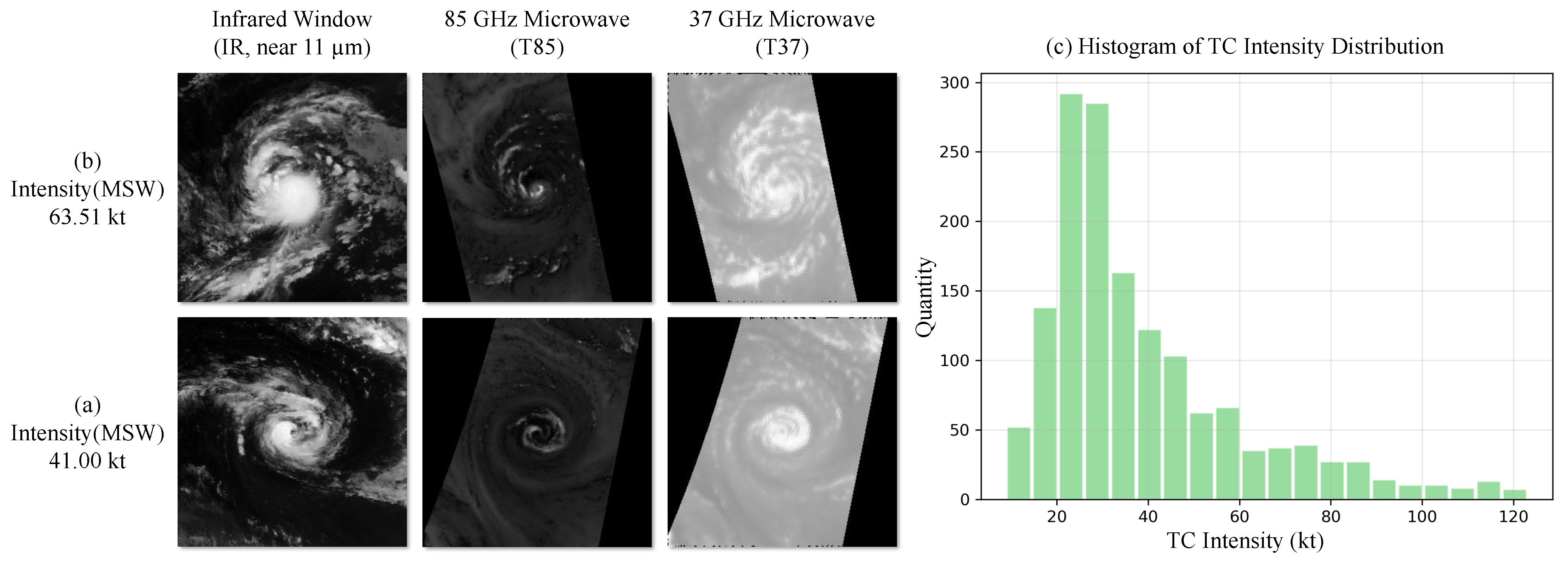
• HURSAT-B1 data are employed for collecting infrared images of TCs. The data covers the time span from 1978 to 2015, with a resolution of 8 km and a 3 h interval, encompassing global TCs. The IRWIN (infrared window, near 11 µm) channel from this dataset is utilized for the MTCID dataset’s infrared images in this study.
• HURSAT-MW data offers microwave images of TCs through passive microwave observations. The dataset includes a total of 2412 TC microwave images from 1987 to 2009, sharing the spatial resolution of HURSAT-B1. In this study, the 37 GHz (T37) and 85 GHz (T85) microwave channels are applied as microwave images for the MTCID dataset. This selection is motivated by the influential nature of the 85–92 GHz frequency range in the model, with the inclusion of 37 GHz providing marginal benefits [11].

2.1.2. Construction of the MTCID Dataset

Through matching longitude and latitude with time, we paired TC infrared images and microwave images taken by HURSAT-B1 and HURSAT-MW at the same time and location. This process created the original images for the MTCID dataset, with an image size of 301 × 301 (cropped to 300 × 300 for calculation). Figure 1a,b display two data examples.

The intensity data of TCs is derived from the global best track maximum sustained wind speed (MSW). We embed the intensity size corresponding to each TC image into the image name, ensuring one-to-one correspondence. While using the estimated best track MSW as the ground truth may not be optimal due to some values lacking on-site confirmation, it is necessary to maintain a large sample of relatively homogeneous data [32]. The unit of intensity size is the knot (kt), internationally recognized by the International Hydrographic Organization, where 1 kt = 0.514 m/s. The data processing steps are as follows:

• The dataset contains numerous images with black patches that do not convey any information about hurricanes, which could complicate the learning process. Hence, images with over 40% invalid information are chosen for elimination through ratio computation.
• As microwave data are captured in a striped pattern by polar-orbiting meteorological satellites, images with scanning coverage less than 60% of the image frame are directly discarded. Moreover, each data point ranges from 0 to 350 as a decimal, and empty values in the data are filled with the maximum value (350, consistent with the background value).
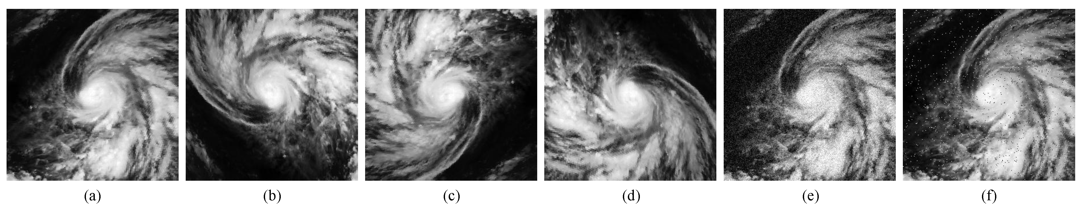
• Due to the intrinsic long-tailed nature of the data (more mid–low intensity TCs and fewer high-intensity TCs), Figure 1c illustrates the intensity distribution of the TC dataset. In this study, some data augmentation approaches are utilized to balance the dataset and alleviate its long-tail effects. We generate additional high-intensity TC data through operations like random rotation and adding noise, as depicted in Figure 2 illustrating the employed data augmentation methods.

Ultimately, we acquired around 15,000 pairs of infrared images, microwave images, and corresponding TC intensity data. The data was partitioned into training, validation, and test sets in an 8:1:1 ratio randomly.

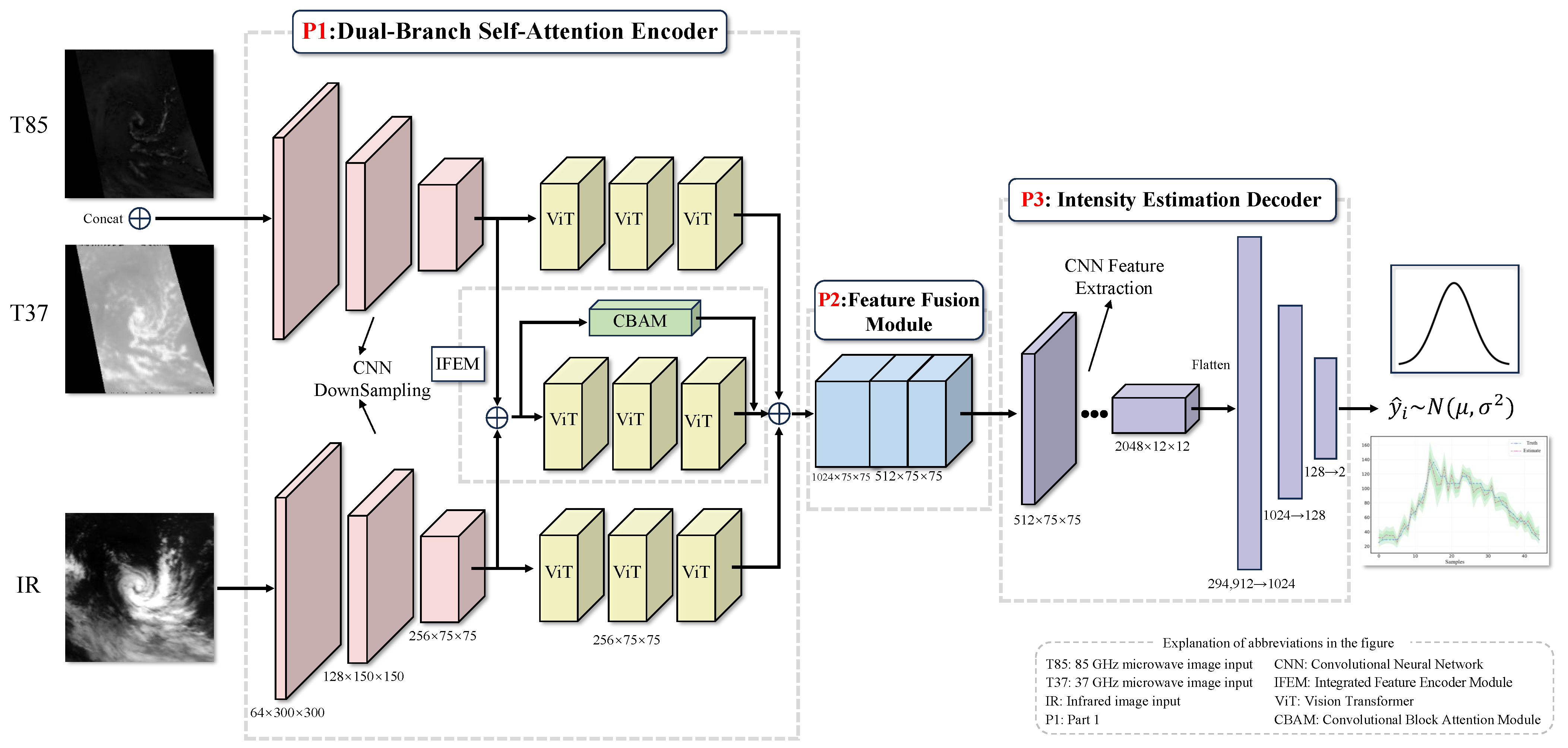
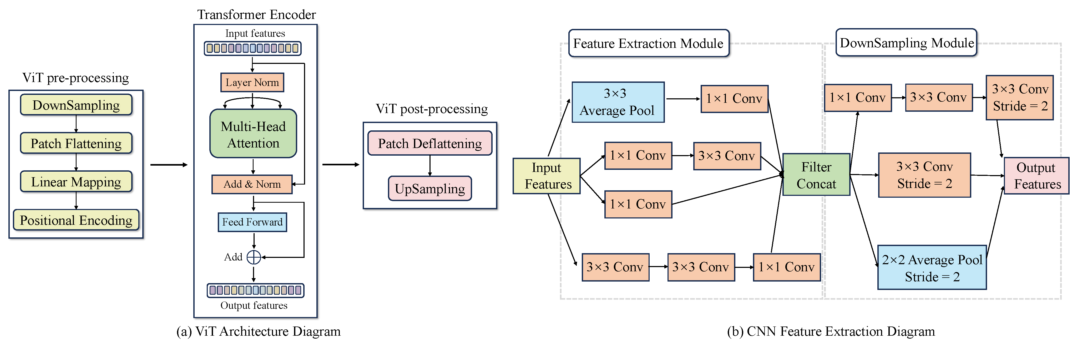
2.2. TC Intensity Probability Estimation Network

Deep learning architectures like CNNs are used to extract features from TC remote sensing images, nonlinearity is introduced by incorporating activation functions (e.g., ReLU), and ultimately TC intensity is obtained through the output layer. This represents the mainstream approach in current deep learning for TC intensity estimation, generally given by the following simplified formula:

$$\left[\widehat{y}\right]=f\left(x\right),$$

(1)

where x represents the input image, $f\left(x\right)$ represents the deep learning model, and $\widehat{y}$ represents the result of TC intensity estimation.

However, many existing methods primarily use a single-source image for TC intensity estimation, not fully leveraging the diverse features of multiple satellite sources. Therefore, this paper introduces a dual-branch self-attention network for TC intensity estimation based on infrared and microwave images (MTCIE), as illustrated in Figure 3.

The model comprises a dual-branch self-attention encoder, feature fusion module, and intensity estimation decoder. The fundamental concept involves using a dual-branch network to extract primary features of microwave and infrared images, incorporating a frequency-domain attention mechanism to strengthen crucial features (P1 in Figure 3). Subsequently, the feature fusion module combines the two sets of features (P2 in Figure 3), and the merged features are further compressed and interpreted to yield TC intensity (P3 in Figure 3). It is important to note that this study, alongside providing deterministic estimates of TC intensity ($\widehat{y_i}$), also captures the standard deviation of the results ($\sigma$), representing probability estimates. This is of particular value in predicting uncertainty in chaotic systems. The model can be simplified as follows:

$$\left[\widehat{y},{\sigma }^2\right]=f\left(x_{IR},x_{MW}\right),$$

(2)

where $x_{IR}$ denotes TC infrared images, $x_{MW}$ represents microwave images, $\widehat{y}$ signifies the accurate value of intensity estimation, and $\sigma$ represents the standard deviation. The following sections will sequentially introduce each module of the network.

2.2.1. Dual-Branch Self-Attention Encoder

Given that this study employs multi-source satellite TC infrared and microwave images as inputs to the model, a straightforward addition or concatenation technique would fail to effectively extract and integrate the diverse features from both sources. Consequently, we opt for a dual-branch network to independently process the two sets of images, efficiently merging diverse information by learning distinct feature representations in each branch. Furthermore, a dual-branch network is well-suited to address the diversity and complexity inherent in multi-source data. This imparts greater robustness to the network against noise, deformations, or other interference factors, rendering it more stable and facilitating easier convergence during model training.

As depicted in Figure 3 P1, the image undergoes three layers of common CNN for downsampling, reducing the size of feature maps. The convolutional kernels of the encoder are 7, 3, 3, and the final output feature map size is denoted as $R^{256\times 75\times 75}$. Subsequently, features pass through three Vision Transformers (ViT) [33] for feature learning. The detailed architecture of ViT is depicted in Figure 4a, encompassing common preprocessing stages (DownSampling, Patch Flattening, Linear Mapping, and Positional Encoding), a transformer encoder with Multi-Head Attention, and post-processing stages (Patch Deflattening and UpSampling).

Furthermore, the model includes an Integrated Feature Encoder Module (IFEM) in the middle, where the ViT architecture aligns with the two branches but incorporates the Convolutional Block Attention Module (CBAM). By incorporating channel and spatial attention mechanisms, CBAM directs the network’s attention towards important channels and spatial positions, thereby improving feature representation. In this context, CBAM integrates features from both infrared and microwave sources at the channel level and concentrates on spatial positions to identify critical components such as the eyewall and spiral rainbands of the TCs. This aids the network in capturing critical information within the TCs, improving overall model performance.

2.2.2. Feature Fusion and Intensity Estimation

Following the concatenation of features from different branches, the feature map proceeds to the feature fusion module (FFM). Common feature fusion methods include addition fusion, maximum value fusion, and convolutional fusion. This study utilizes convolutional fusion, allowing the network to learn how to combine features from different sources in a more complex manner. The network architecture is inspired by Residual CNN [34]. The features first undergo two common CNN convolutional identity mapping processes (3 × 3 conv, BatchNorm, and ReLU activation) for feature fusion. Subsequently, a Residual Connection captures the difference between the input and output, followed by another ReLU activation. This process is repeated three times to ensure thorough feature fusion.

After preceding feature extraction and fusion, stable fused features enter the intensity estimation decoder. Firstly, there are three CNN feature extraction blocks, inspired by the Inception V3 module [35], which aids in multi-scale feature extraction to improve parameter and computational efficiency, as depicted in Figure 4b. Readers can try modifying it with other models to enhance performance but this is not the primary focus of the current research. Subsequently, the features are flattened and, after traversing three fully connected layers, the final outputs for intensity and standard deviation are obtained.

2.2.3. Loss Function

Due to the complexity, nonlinearity, and chaotic effects of the Earth system, there is inherent uncertainty in TC intensity estimation [36]. It is commonly assumed that the errors in TC intensity estimation follow an approximate normal distribution, with a mean close to zero. To fully capture the uncertainty in multimodal TC data, the output of this study’s model is modeled as a Gaussian distribution. In other words, the model learns to predict both the mean and standard deviation of the dependent variable, providing more accurate predictions.

Typically, intensity estimation deep learning models use the Mean Squared Error (MSE) loss function to achieve precise intensity estimates, as shown in Equation (3). This study requires two sets of outputs: one set is the final predicted results ($\widehat{y}$) and the other set is the uncertainty standard deviation of the results ($\widehat{\sigma }$). Therefore, the loss function used is shown in Equation (4).

$$Loss=\frac{1}{N}\sum _i{∥y_i-{\widehat{y}}_i∥}^2,$$

(3)

$$Loss=\frac{1}{N}\sum _i\frac{1}{2}{\widehat{\sigma }}_i^{-2}{∥y_i-{\widehat{y}}_i∥}^2+\frac{1}{2}log{\widehat{\sigma }}_i^2,$$

(4)

where N represents the number of samples and i is the index of the image. The loss function illustrated in Equation (4) comprises two components: one is the residual of the regression model, aimed at capturing the cognitive uncertainty of model parameters; the other is the aleatoric uncertainty of the estimated results, serving as a regularization term [37]. It is noteworthy that, when learning aleatoric uncertainty, there is no need to annotate the true values for the standard deviation $\widehat{\sigma }$ separately. This is because, during the minimization of the loss function, the size of the standard deviation will adaptively adjust.

3. Experimental Results

3.1. Experimental Setup and Evaluation Metrics

All models in this study are implemented using the PyTorch framework. The initial learning rate is set to 0.0002, the Adam optimizer is selected, and the learning rate is gradually decreased during training. The batch size is set to 4. Our experimental and validation environment is as follows: an Intel Core i9-9900K CPU, 128 GB RAM, and a Geforce RTX 3090 GPU, with the operating system being Ubuntu 18.04.

3.1.1. Deterministic Estimation Metrics

To assess the performance of the model’s deterministic estimation, the study adopts the current mainstream metrics, namely, Mean Absolute Error (MAE) and Root Mean Square Error (RMSE), to calculate the errors between the estimated values and the ground truth.

$$MAE=\frac{1}{N}\sum _{i=1}^N\left|y_i-{\widehat{y}}_i\right|,$$

(5)

$$RMSE=\sqrt{\frac{1}{N}\sum _{i=1}^N{\left(y_i-{\widehat{y}}_i\right)}^2},$$

(6)

where N represents the number of samples, $\widehat{y}$ represents the deterministic TC intensity estimate, y represents the true intensity value, and i is the index of the image.

3.1.2. Probabilistic Estimation Evaluation Metrics

To evaluate the performance of the model’s probabilistic estimation, the study adopts the Continuous Ranked Probability Score (CRPS), where a smaller CRPS indicates better overall performance in probability prediction. The formula for CRPS based on a normal distribution ($\mu ,\sigma$) is as follows:

$$CRPS\left(x,y\right)=\sigma \left\{\omega \left[2\mathsf{\Phi }\left(\omega \right)\right]+2\varphi \left(\omega \right)-\frac{1}{\sqrt{\pi }}\right\},$$

(7)

where $\omega =(y-\mu )/\sigma$, and $\mathsf{\Phi }$ and $\varphi$ represent the probability density function (PDF) and cumulative distribution function (CDF) of the standard normal distribution, respectively.

To assess the usability of interval predictions, the study applies the Prediction Interval Coverage Probability (PICP) and the Mean Width Percentage (MWP). ${PICP}_{\alpha }$ is the probability of observed values falling within the predicted interval at a confidence level $\alpha$ and ${MWP}_{\alpha }$ represents the width of the interval. High PICP and low MWP are generally considered ideal for interval prediction performance. By default, a 95% confidence interval is used to compare interval metrics.

$${PICP}_{\alpha }=\frac{c_{\alpha }}{m}\times 100\%,$$

(8)

$${MWP}_{\alpha }=\frac{1}{m}\sum _{i=1}^m\frac{{up}_i-{down}_i}{{\widehat{y}}_i},$$

(9)

where $c_{\alpha }$ is the number of samples with observed values falling within the predicted interval.

3.2. Ablation Experiment Results

Different module designs and inputs from different sources can have a significant impact on experimental results. Therefore, this study primarily conducts two types of ablation experiments to validate the effectiveness of the model and find the optimal model configuration.

3.2.1. Module Ablation Experiment for MTCIE

In this section, ablation experiments were conducted on the module design of MTCIE. In

Table 1. Results of module ablation experiment. ✓ indicates the presence of the module and the best results are highlighted in bold.

Modules				Metrics
Baseline	ViT	IFEM	FFM	MAE↓ (kt)	RMSE↓ (kt)
✓				8.34	10.48
✓	✓			7.93	9.83
✓	✓	✓		7.51	9.35
✓	✓	✓	✓	7.42	9.25

, “Baseline” denotes a standard dual-branch structure composed of CNNs, “ViT” signifies replacing the CNNs in the dual-branch encoder with a ViT encoder, “IFEM” refers to inserting ViT Blocks with CBAM in the middle of the dual-branch encoder (Figure 3 P1), and “FFM” is employed for feature fusion just before the intensity estimation decoder (Figure 3 P2). Table 1 shows the MAE and RMSE performance of different module combinations on the test set. The results indicate that the introduction of the three modules has helped improve the accuracy of intensity estimation. Looking at the MAE and RMSE metrics, the ViT module and IFEM module show significant improvements, both around 5%, while FFM, relatively speaking, has a smaller improvement, only about 1%. We speculate that, as the model already has relatively good performance, further improvement enters a saturation stage, making performance enhancement more challenging.

In Table 1, “Baseline” denotes a standard dual-branch structure composed of CNNs, “ViT” signifies replacing the CNNs in the dual-branch encoder with a ViT encoder, “IFEM” refers to inserting ViT Blocks with CBAM in the middle of the dual-branch encoder, and “FFM” is employed for feature fusion just before the intensity estimation decoder.

3.2.2. Ablation Experiment for Multiple Source Image Inputs

To validate the intensity estimation effect of TC images from different satellite sources, we conducted ablation experiments on different image inputs. Here, IR represents infrared images from geostationary meteorological satellites, T37 represents images from the 37 GHz microwave channel of polar-orbiting meteorological satellites, and T85 represents images from the 85 GHz microwave channel. When experimenting with a single-source image, we removed one branch of the dual-branch model. To minimize the impact of changes in the model structure on the experiment, we retained the CBAM attention mechanism module and FFM feature fusion module. Four different models were trained for different scenarios and the best-performing model (on the validation set) was selected to represent each scenario.

The final experimental results are shown in

Table 2. Experiment on ablation of input data. IR, T37, and T85 represent the infrared, 37 GHz microwave, and 85 GHz microwave images, respectively. ✓ indicates the presence of the data and the best results are highlighted in bold.

Input Data			Metrics
IR	T37	T85	MAE↓ (kt)	RMSE↓ (kt)
✓			7.95	9.87
	✓		12.48	14.35
		✓	10.67	12.62
✓	✓		7.84	9.74
✓		✓	7.51	9.38
✓	✓	✓	7.42	9.25

. It can be seen that infrared images play the most crucial role in the intensity estimation of TCs. This is because infrared images usually contain information such as the cloud-top temperature and cloud structure of TCs. For stronger TCs, infrared remote sensing images can also display the formation and development of the eyewall. This information is often closely related to the intensity of TCs, which is one of the reasons why scientists initially used infrared remote sensing images to study TC intensity.

The 85 GHz microwave channel (T85) is slightly inferior to the infrared channel (IR), while the 37 GHz microwave channel (T37) is the least effective. From Table 2, it is evident that the intensity estimation results obtained from using only the T37 as model input are less effective compared to T85. The intensity estimation performance experiences a substantial improvement after the inclusion of IR data. Nevertheless, the combination of IR and T85 continues to outperform the combination of IR and T37. Consequently, it can be inferred that the 85 GHz images contain a greater amount of intensity-related information compared to the 37 GHz images. This experimental outcome aligns with the findings of Wimmers [11]. However, overall, the effect of microwave images on intensity estimation is still significantly different from that of infrared images. When all multiple-source images are input together, the best results are obtained. This indicates that microwave images can supplement information that infrared images may not capture, contributing to a more comprehensive understanding of TCs by the model.

3.3. Deterministic Estimation Experiments

The model used in this study introduces uncertainty, and the model output includes both the mean and standard deviation, representing probability estimates. Of course, it can also be directly understood as deterministic intensity estimation and the error range of uncertainty. This section primarily verifies the experimental effectiveness of deterministic estimation by the model.

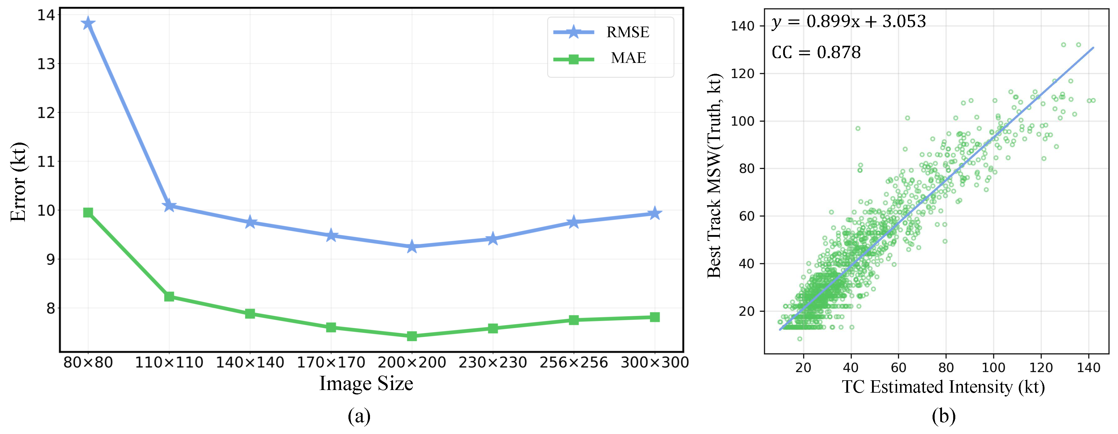
3.3.1. Input Image Size Comparative Experiment

In our study, we found that TC images captured by satellites are centered around the eyewall, with a fixed window size covering the entire TC. This leads to significant differences in coverage relative to the entire image for TC cloud images of different sizes and shapes. The most valuable information about cyclone intensity is typically located near the center. Therefore, different image sizes obtained through cropping will have different effects. Secondly, since microwave images are obtained by polar-orbiting satellites, the images are striped, and there is some information loss compared to infrared images. Different image sizes will also affect the balance between effective information and interference information in microwave images.

The experimental results are shown in Figure 5a. It can be seen that, when reducing the input image size, some noise or interference information can be physically excluded, allowing the model to focus more deeply on extracting valid information to improve performance. However, the gains from this approach will disappear after reducing the image to a certain extent and it may have a negative impact due to the loss of too much image information, especially when reducing to around 80 × 80. The optimal image size we obtained is around 200 × 200. Since there are a large number of different experimental configurations here, there may be other optimal image sizes, but this is not the focus of this study.

3.3.2. Test Dataset Quantitative Evaluation Experiment

In the study, around 1500 TC images from the test set were estimated. Figure 5b displays a scatter plot comparing the deterministic estimation of TC intensity with the actual values. The blue line represents the linear fit between the estimated intensity and actual wind speed, and the figure includes the formula of the fitted line and the correlation coefficient (CC).

The scatter plot reveals that, when estimating TC wind speeds below approximately 30 kt, corresponding to tropical depressions, our TC intensity estimates tend to be higher (leaning towards the bottom right). A similar pattern occurs when the wind speed exceeds around 120 kt, while, in the intermediate wind speed range, the distribution is relatively uniform. We hypothesize that the model, when estimating extreme values, tends to overestimate to reduce errors. We posit that adopting an inclination towards estimating worst-case scenarios is beneficial in real-world situations, particularly during erroneous estimations, to mitigate losses induced by TCs.

Additionally, due to the long-tail effect in data distribution, the scatter plot has more sample points at low wind speeds and the distribution is denser, concentrated around the diagonal with a slope of 1. This indicates that the model’s accuracy is higher with smaller standard deviations when predicting low wind speeds and the opposite is observed at high wind speeds.

For a more comprehensive analysis of the model’s deterministic estimation performance, we categorized the TC intensity in the test set. As the World Meteorological Organization has different standards for TC classification in different ocean regions, we followed the standards for the Northwest Pacific. The results of the model’s actual estimation of TC intensity by category are presented in

Table 3. Intensity deterministic estimation results categorized by TC types, classified according to the Northwest Pacific standards as Tropical Depression (TD), Tropical Storm (TS), Severe Tropical Storm (STS), Typhoon (TY), Severe Typhoon (STY), and Super Typhoon (Super TY). The best results are highlighted in bold. The ↓ indicates that a lower value represents better performance.

	Range of Wind Speed (kt)	Sample Size	MAE↓ (kt)	RMSE↓ (kt)
TD	≤33.25	478	6.67	8.47
TS	33.45–47.45	332	6.72	8.58
STS	47.64–63.32	256	7.61	9.47
TY	63.52–80.47	198	8.17	10.03
STY	80.73–98.79	157	9.05	11.14
Super TY	≥99.13	88	10.68	12.75
Average			7.42	9.25

.

Overall, the model demonstrates good performance in deterministic estimation of TC intensity, comparable to current mainstream models. It is noteworthy that the model exhibits better accuracy in estimating the intensity of weaker TCs (TD and TS) compared to more intense ones, such as severe typhoons (STYs) and super typhoons. This aligns with the observations in Figure 5b. We speculate that the limited data for higher-intensity TCs may result in suboptimal model training, requiring further improvement in estimation accuracy. Additionally, high-intensity TCs usually have more complex internal structures and may undergo more transient processes, adding to the difficulty of estimating their intensity.

3.3.3. Comparative Experiments in Deterministic Estimation

This section compares several mainstream TC intensity estimation methods, including DeepMicroNet [11], TCIENet [38], Deep-PHURIE [10], TCICENet [39], and DMANel_KF [21]. The results are shown in

Table 4. Comparative experiments with other mainstream models on deterministic estimation. The ↓ indicates that a lower value represents better performance.

Models	Data	MAE↓ (kt)	RMSE↓ (kt)	References
DeepMicroNet	MINT	-	10.60	[11]
TCIENet	IR, WV	7.84	9.98	[38]
Deep-PHURIE	IR	7.96	8.94	[10]
TCICENet	IR	6.67	8.60	[39]
DMANel_KF	IR1, IR2, IR3, IR4	6.19	7.82	[21]
MTCIE	IR, T37, T85	7.42	9.25	Ours

. To be precise, directly comparing our model with others is unfair because different models use different datasets. Additionally, since our data come from multiple satellites, reproducing other models on our dataset is challenging. However, to demonstrate the performance of our method, we still compare it with the estimation results of other researchers. From the table, although our model did not achieve the best performance in terms of RMSE and MAE metrics, it still controlled the errors within a reasonable range and could compete with current mainstream models in deterministic forecasting.

We speculate that two factors limit the model’s deterministic prediction capability. First, the influence of probability estimation affects the performance of deterministic estimation. Since the model’s estimation results include both deterministic intensity values and the standard deviation of uncertain estimation, the two mutually affect each other, as reflected in the loss function shown in Formula (4). Therefore, the model’s deterministic estimation tends to be conservative and cautious, balancing with probability estimation. Second, data quality limits the model’s performance. As our data comes from paired infrared and microwave images from multiple satellites, there are issues such as misalignment and data sparsity. Compared with other homogeneous and homologous datasets, the data quality is not high. We speculate that these two main reasons limit the model from achieving better MAE and RMSE metrics in deterministic estimation.

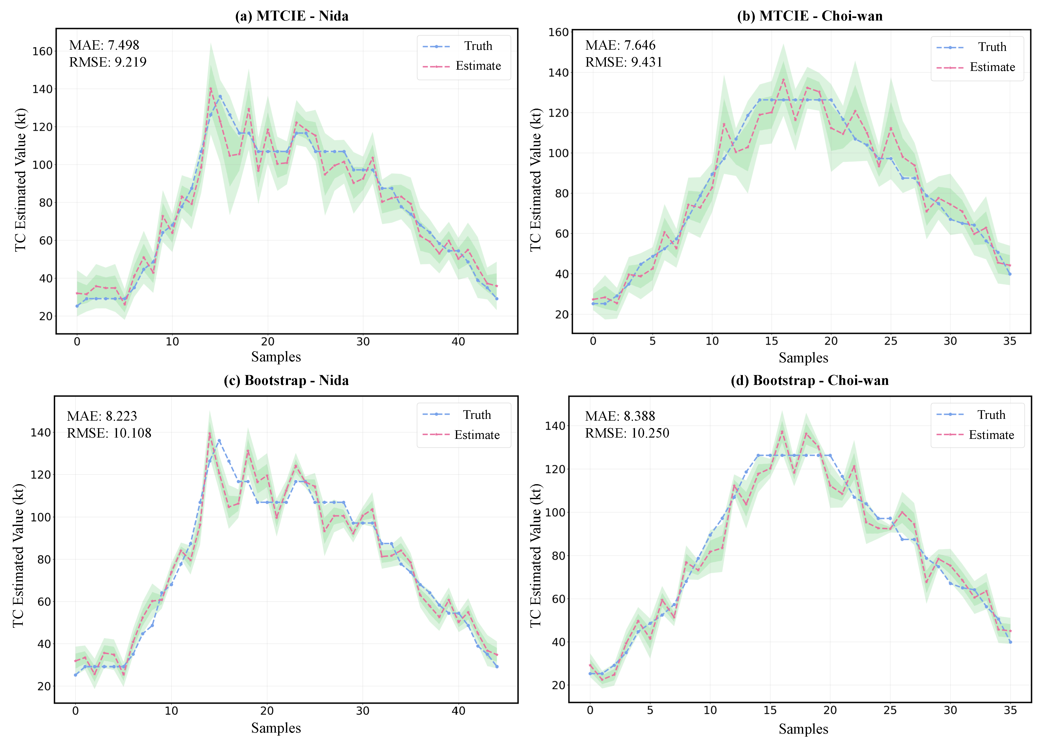
3.4. Probability Estimation Experiments

3.4.1. Comparative Experiment of Probability Estimation

This section compares various models’ performance in probability estimation (uncertainty estimation). We evaluated some of the most popular uncertainty estimation models, including MC Dropout [23], Deep Ensemble(DE) [40], Quantile Regression (QR) [41], and Bootstrap [42]. The results are presented in

Table 5. Comparative experiments with other mainstream models on probabilistic estimation. The best results are highlighted in bold. The ↓ indicates that a lower value represents better performance. The ↑, on the contrary, signifies the opposite.

Models	MAE↓ (kt)	RMSE↓ (kt)	CRPS↓	PICP↑	MWP↓
MC Dropout	9.74	11.39	2.18	0.487	0.235
DE	8.81	10.60	3.43	0.916	0.781
QR	11.35	13.26	-	0.258	0.574
Bootstrap	7.83	9.87	1.76	0.445	0.139
Ours	7.42	9.25	2.45	0.958	0.925

.

Overall, regarding deterministic evaluation metrics such as MAE and RMSE, as well as probability estimation metrics like PICP, the MTCIE model exhibits relatively superior performance. However, for CRPS and MWP metrics, the Bootstrap model outperforms others. It is noteworthy that the QR model’s performance differs significantly from other models, performing almost the worst in all metrics.

In terms of the CRPS metric, the Bootstrap model demonstrates the best performance, while the MC Dropout and MTCIE metrics are slightly less favorable. We speculate that this is because Bootstrap introduces uncertainty through simple random resampling, a method that aligns well with the normal distribution, making the CRPS metric calculation more fitting. In contrast, MC Dropout introduces randomness by randomly deactivating neurons and MTCIE constrains the model’s direct output uncertainty through the loss function. The uncertainty outputs of the latter two do not align as well with the CRPS metric calculation as Bootstrap, resulting in relatively poorer performance.

Therefore, we also introduced a joint comparison of the PICP and MWP metrics, providing a more comprehensive analysis of the model’s interval prediction and probability estimation. In terms of interval coverage (PICP), MTCIE performs the best, achieving close to a 96% interval coverage rate in most cases. Although the Deep Ensemble model also has a 91% interval coverage rate, its performance in deterministic forecasting is poor. When considering interval width (MWP), it is evident that MTCIE consistently exhibits the widest intervals, which may not be user-friendly in practical applications. In comparison, Bootstrap has the best MWP metric but the generated interval coverage range is too narrow, making it unable to capture actual values and resulting in a low interval coverage rate (PICP), less than 50%. We speculate that this is consistent with the high CRPS metric, indicating that this method relies entirely on data selection without considering sufficient uncertainty. Such overconfident estimates are not very practical in TC intensity estimation.

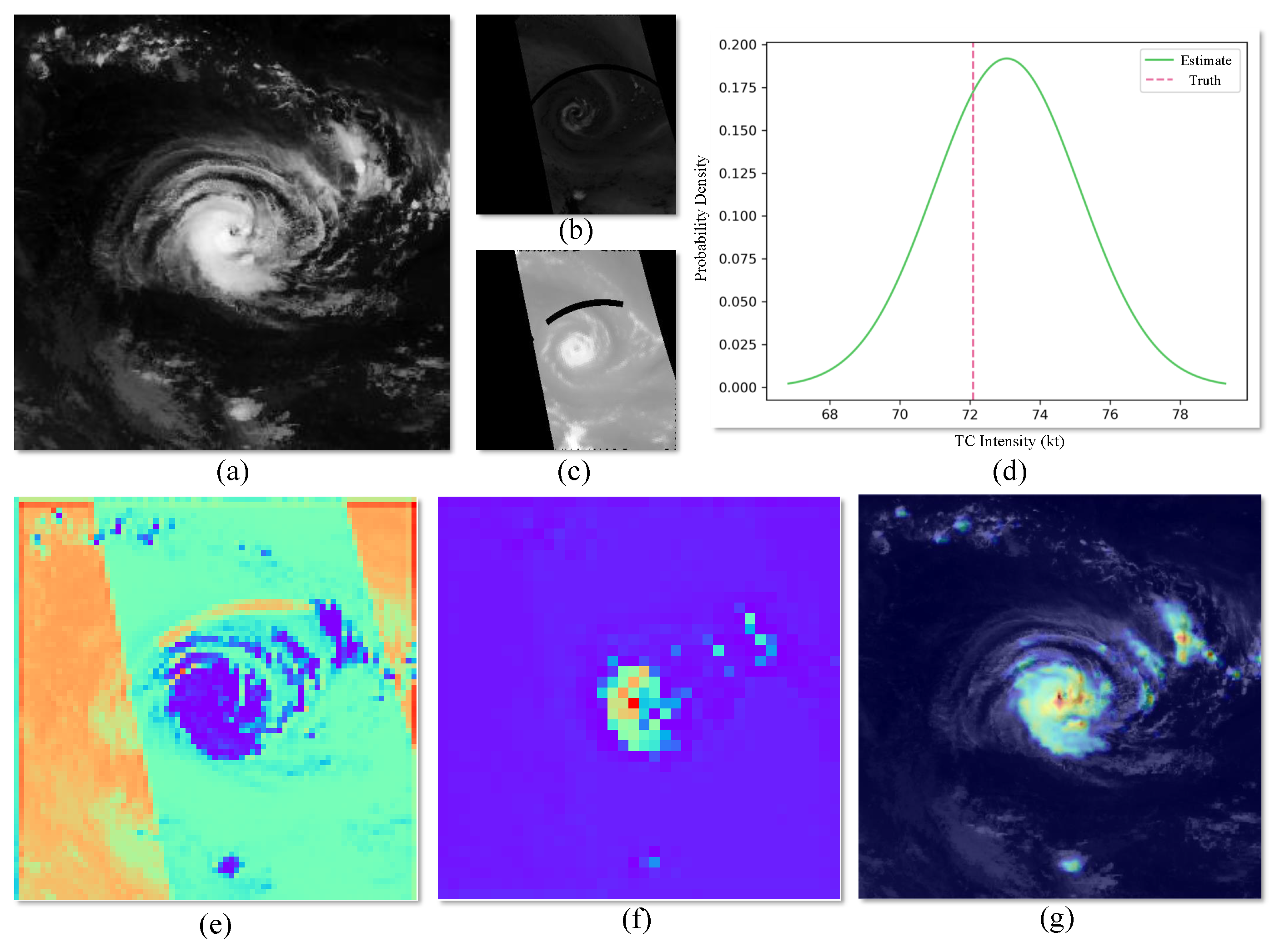
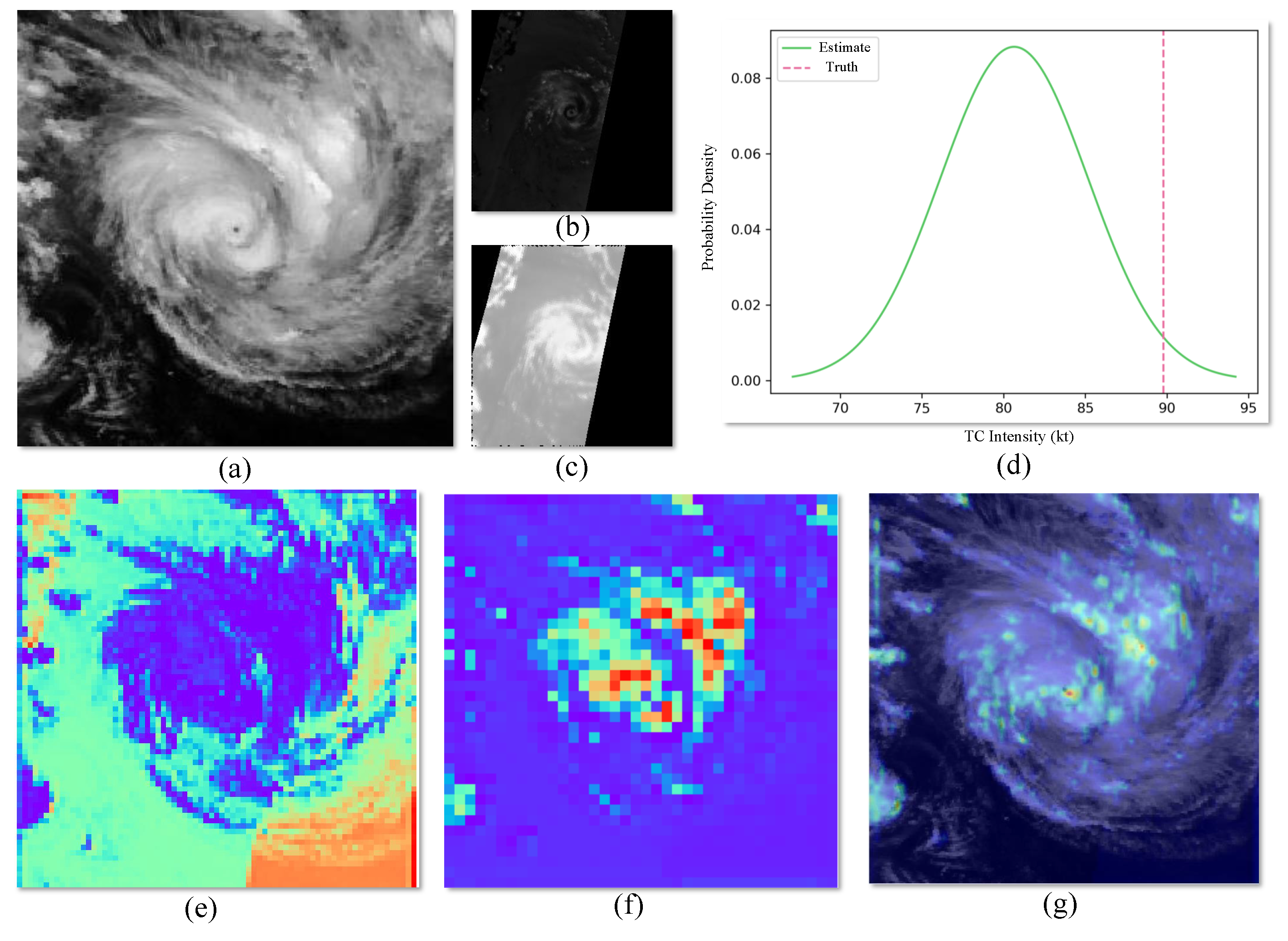
3.4.2. Individual Case Experiment

For independent validation, we chose two typical TCs. Figure 6 depicts the intensity variations of two significant TCs, “Nida” and “Choi-wan”, impacting the northwest Pacific in 2009. It showcases the intensity values along the best track (ground truth), our estimated intensities, and the associated uncertain estimation intervals. To assess the efficacy of probabilistic forecasting, we compare Bootstrap (Figure 6c,d) with our MTCIE model (Figure 6a,b).

From Figure 6a,b, it can be seen that our model has a good deterministic estimation of TC intensity but the error is larger at higher TC intensities than at lower intensities. This is reflected in the sudden overestimation or underestimation of the model’s results when estimating high-intensity TCs. Correspondingly, the uncertainty estimation also increases in such high-intensity TC estimations, reflecting an increase in the interval of uncertainty estimation. We believe this may be due to the small sample size of high-intensity TCs in the dataset, coupled with the fact that high-intensity TCs usually have more complex structures and variations, leading to an increase in the model’s estimated uncertainty.

Figure 6c,d reveal that the TC intensity determinacy estimation results from Bootstrap are somewhat less favorable compared to MTCIE. Furthermore, in line with Table 5, while Bootstrap demonstrates relatively narrow interval widths in uncertainty estimation, aiding clearer decision making in practical applications, its interval coverage rate is low. Such overconfidence can lead to significant errors, especially in the context of severe natural disasters like TCs, which is deemed unacceptable.

Additionally, in Figure 6a,b, for extreme TCs with wind speeds below 30 kt and above 120 kt, the model tends to make overestimations, consistent with the scatter plot in Figure 5b. It is worth noting that the uncertainty estimation results here almost completely cover the actual values, indicating that MTCIE can play an important role in actual risk decision making. In high-intensity TC forecasting, uncertainty estimation can make intensity estimation more flexible, facilitating adjustments to the next preventive strategy and enhancing risk resilience.

4. Discussion

4.1. Misestimation Analysis

Deep learning models are often considered black-box structures, meaning that the mapping relationship between input and output is difficult to understand intuitively. This makes the model’s decision-making process opaque to external observers. Therefore, explaining the reasons for the model’s incorrect or correct estimates is challenging. In this section, we attempt to analyze the reasons for the model’s inaccurate estimation of certain TC intensities by visualizing the feature layers.

We identified two TC intensity estimation cases in the test set and analyzed the decision-making process of their intensity estimates through feature layer visualization and activation heatmaps. The experimental results are shown in Figure 7 and Figure 8, where the former is a case of accurate TC intensity estimation, while the latter is a case of less accurate estimation.

In Figure 7 and Figure 8, (a–c) represent the input IR, T85, and T37 images. (f) shows the comparison between the model’s output probability estimates and the ground truth, indicating that the probability estimates in the case of Figure 7 are better than those in Figure 8.

(e) represents the results of one channel after the first ViT feature extraction in the IFEM module. It can be observed that the model starts to fuse features from different sources and captures the essential core region of the cloud image. The stripes from the polar-orbiting satellite are still clearly visible at this stage. (f) represents the results after the FFM module, showing one channel of the feature map after the first feature extraction downsampling in the decoder. At this point, features from multiple sources have completely fused and focus on crucial areas such as the TC’s eyewall, spiral rainband, and mid-level cloud band. (g) displays the visualized activation heatmap, indicating which content has a greater impact on the image’s estimation result (red areas represent high impact, purple areas represent low impact).

From (f,g), we identified possible reasons for the model’s estimation errors. It can be seen that the TC intensity in successful cases is not too high compared to failed cases; the former’s cloud structure is relatively simple and the model focuses on the vicinity of the eyewall. However, in failed cases, the cloud structure is more complex, with strong cloud systems on the upper right side of the eyewall, causing a shift in the model’s attention and resulting in significant estimation errors. Of course, this is just a preliminary analysis of possible error causes, and further professional analysis and improvement measures are the focus of our next research steps.

4.2. Limitations

This study represents an initial attempt at the probabilistic estimation of TC intensity using multi-source satellite images and, therefore, there are certain limitations. Here, we briefly list a few for further exploration by other researchers.

• The quality and size of the dataset need improvement. The data obtained through pairing are limited and there is a certain misalignment. Additionally, the dataset distribution is highly uneven, displaying a significant long-tail effect. While data augmentation measures alleviate this issue to some extent, more, higher-quality, balanced data are still required.
• The estimation performance for high-intensity TCs is unsatisfactory. Although probabilistic estimation enlarges uncertainty to constrain results within the estimated range, improving both deterministic and probabilistic estimation can be achieved by incorporating more data and expert knowledge on high-intensity TCs.
• Although the probabilistic estimation results cover a majority of real scenarios, the estimated interval width is relatively large, leaving room for improvement in practical applications.

5. Conclusions

In this paper, the uncertainty introduced by multi-source data input and the intrinsic chaotic nature of TCs necessitate a model capable of quantitatively estimating uncertainty. Therefore, we introduce the Multi-source satellite image-based TC Intensity Estimation (MTCIE) model, representing the first known application of uncertainty in TC intensity estimation. By fully leveraging current multi-source satellite resources, we use TC’s infrared and microwave images as inputs to a dual-branch network. The neural network extracts TC features separately and, after feature fusion, provides probabilistic estimates of intensity. In addition to deterministic intensity estimates, we also provide estimated standard deviations, which can be presented in the form of estimated intervals or confidence intervals in practical applications.

Experimental results on the proposed Multi-source TC Intensity Estimation Dataset (MTCID) show that the MTCIE model performs comparably well in deterministic forecasting to current mainstream methods and outperforms comparative models in probability estimation and interval prediction. Moreover, the study of two typhoon cases in 2009 indicates that our model’s probabilistic estimation intervals can almost perfectly cover the actual values. In subsequent discussions, we utilize feature layer visualization and activation heatmap visualization to briefly analyze the reasons for model estimation errors, and present the current model’s limitations. In summary, the application of MTCIE in TC intensity probabilistic estimation is expected to provide assistance in hurricane warnings, disaster management, emergency decision making, and other operational areas. Future research will explore the integration of transfer learning and physical mechanisms into multi-source image-based TC intensity probabilistic estimation to enhance its performance.

References

1. Dominguez, C.; Magaña, V. The role of tropical cyclones in precipitation over the tropical and subtropical North America. Front. Earth Sci. 2018, 6, 19. [Google Scholar] [CrossRef]
2. Swain, D. Tropical cyclones and coastal vulnerability: Assessment and mitigation. Geospat. Technol. Land Water Resour. Manag. 2022, 103, 587–621. [Google Scholar]
3. Velden, C.; Harper, B.; Wells, F.; Beven, J.L.; Zehr, R.; Olander, T.; Mayfield, M.; Guard, C.; Lander, M.; Edson, R.; et al. The Dvorak tropical cyclone intensity estimation technique: A satellite-based method that has endured for over 30 years. Bull. Am. Meteorol. Soc. 2006, 87, 1195–1210. [Google Scholar] [CrossRef]
4. Yang, Y.; Zhang, J.; Bao, Z.; Ao, T.; Wang, G.; Wu, H.; Wang, J. Evaluation of multi-source soil moisture datasets over central and eastern agricultural area of China using in situ monitoring network. Remote Sens. 2021, 13, 1175. [Google Scholar] [CrossRef]
5. Mohammadpour, P.; Viegas, C. Applications of Multi-Source and Multi-Sensor Data Fusion of Remote Sensing for Forest Species Mapping. Adv. Remote Sens. For. Monit. 2022, 255–287. [Google Scholar] [CrossRef]
6. Shao, Z.; Pan, Y.; Diao, C.; Cai, J. Cloud detection in remote sensing images based on multiscale features-convolutional neural network. IEEE Trans. Geosci. Remote Sens. 2019, 57, 4062–4076. [Google Scholar] [CrossRef]
7. Panegrossi, G.; D’Adderio, L.P.; Dafis, S.; Rysman, J.F.; Casella, D.; Dietrich, S.; Sanò, P. Warm Core and Deep Convection in Medicanes: A Passive Microwave-Based Investigation. Remote Sens. 2023, 15, 2838. [Google Scholar] [CrossRef]
8. Qiu, S.; Zhao, H.; Jiang, N.; Wang, Z.; Liu, L.; An, Y.; Zhao, H.; Miao, X.; Liu, R.; Fortino, G. Multi-sensor information fusion based on machine learning for real applications in human activity recognition: State-of-the-art and research challenges. Inf. Fusion 2022, 80, 241–265. [Google Scholar] [CrossRef]
9. Wang, C.; Zheng, G.; Li, X.; Xu, Q.; Liu, B.; Zhang, J. Tropical cyclone intensity estimation from geostationary satellite imagery using deep convolutional neural networks. IEEE Trans. Geosci. Remote Sens. 2021, 60, 1–16. [Google Scholar] [CrossRef]
10. Dawood, M.; Asif, A.; Minhas, F.u.A.A. Deep-PHURIE: Deep learning based hurricane intensity estimation from infrared satellite imagery. Neural Comput. Appl. 2020, 32, 9009–9017. [Google Scholar] [CrossRef]
11. Wimmers, A.; Velden, C.; Cossuth, J.H. Using deep learning to estimate tropical cyclone intensity from satellite passive microwave imagery. Mon. Weather Rev. 2019, 147, 2261–2282. [Google Scholar] [CrossRef]
12. Heming, J.T.; Prates, F.; Bender, M.A.; Bowyer, R.; Cangialosi, J.; Caroff, P.; Coleman, T.; Doyle, J.D.; Dube, A.; Faure, G.; et al. Review of recent progress in tropical cyclone track forecasting and expression of uncertainties. Trop. Cyclone Res. Rev. 2019, 8, 181–218. [Google Scholar] [CrossRef]
13. Feng, K.; Ouyang, M.; Lin, N. Tropical cyclone-blackout-heatwave compound hazard resilience in a changing climate. Nat. Commun. 2022, 13, 4421. [Google Scholar] [CrossRef] [PubMed]
14. Marks, F.D.; Shay, L.K.; Barnes, G.; Black, P.; Demaria, M.; McCaul, B.; Mounari, J.; Montgomery, M.; Powell, M.; Smith, J.D.; et al. Landfalling tropical cyclones: Forecast problems and associated research opportunities. Bull. Am. Meteorol. Soc. 1998, 79, 305–323. [Google Scholar]
15. Martin, J.D.; Gray, W.M. Tropical cyclone observation and forecasting with and without aircraft reconnaissance. Weather Forecast. 1993, 8, 519–532. [Google Scholar] [CrossRef]
16. Maral, G.; Bousquet, M.; Sun, Z. Satellite Communications Systems: Systems, Techniques and Technology; John Wiley & Sons: Hoboken, NJ, USA, 2020. [Google Scholar]
17. Velden, C.; Hawkins, J. Satellite observations of tropical cyclones. In Global Perspectives on Tropical Cyclones: From Science to Mitigation; World Scientific: Singapore, 2010; pp. 201–226. [Google Scholar]
18. Lee, J.; Im, J.; Cha, D.H.; Park, H.; Sim, S. Tropical cyclone intensity estimation using multi-dimensional convolutional neural networks from geostationary satellite data. Remote Sens. 2019, 12, 108. [Google Scholar] [CrossRef]
19. Clement, M.; Snell, Q.; Walke, P.; Posada, D.; Crandall, K. TCS: Estimating gene genealogies. In Proceedings of the Parallel and Distributed Processing Symposium, International; IEEE Computer Society: Washington, DC, USA, 2002; Volume 2, p. 7. [Google Scholar]
20. Pradhan, R.; Aygun, R.S.; Maskey, M.; Ramachandran, R.; Cecil, D.J. Tropical cyclone intensity estimation using a deep convolutional neural network. IEEE Trans. Image Process. 2017, 27, 692–702. [Google Scholar] [CrossRef] [PubMed]
21. Jiang, W.; Hu, G.; Wu, T.; Liu, L.; Kim, B.; Xiao, Y.; Duan, Z. DMANet_KF: Tropical Cyclone Intensity Estimation Based on Deep Learning and Kalman Filter From Multi-Spectral Infrared Images. IEEE J. Sel. Top. Appl. Earth Obs. Remote Sens. 2023, 16, 4469–4483. [Google Scholar] [CrossRef]
22. Gawlikowski, J.; Tassi, C.R.N.; Ali, M.; Lee, J.; Humt, M.; Feng, J.; Kruspe, A.; Triebel, R.; Jung, P.; Roscher, R.; et al. A survey of uncertainty in deep neural networks. Artif. Intell. Rev. 2023, 56, 1513–1589. [Google Scholar] [CrossRef]
23. Gal, Y.; Ghahramani, Z. Dropout as a bayesian approximation: Representing model uncertainty in deep learning. In Proceedings of the International Conference on Machine Learning, New York, NY, USA, 19–24 June 2016; pp. 1050–1059. [Google Scholar]
24. Yang, J.Y.; Wang, J.D.; Zhang, Y.F.; Cheng, W.J.; Li, L. A heuristic sampling method for maintaining the probability distribution. J. Comput. Sci. Technol. 2021, 36, 896–909. [Google Scholar] [CrossRef]
25. Jiang, S.H.; Liu, X.; Wang, Z.Z.; Li, D.Q.; Huang, J. Efficient sampling of the irregular probability distributions of geotechnical parameters for reliability analysis. Struct. Saf. 2023, 101, 102309. [Google Scholar] [CrossRef]
26. Kamran, M. A probabilistic approach for prediction of drilling rate index using ensemble learning technique. J. Min. Environ. 2021, 12, 327–337. [Google Scholar]
27. Yang, Y.; Hong, W.; Li, S. Deep ensemble learning based probabilistic load forecasting in smart grids. Energy 2019, 189, 116324. [Google Scholar] [CrossRef]
28. Sun, J.; Wu, S.; Zhang, H.; Zhang, X.; Wang, T. Based on multi-algorithm hybrid method to predict the slope safety factor–stacking ensemble learning with bayesian optimization. J. Comput. Sci. 2022, 59, 101587. [Google Scholar] [CrossRef]
29. Mercer, A.; Grimes, A. Atlantic tropical cyclone rapid intensification probabilistic forecasts from an ensemble of machine learning methods. Procedia Comput. Sci. 2017, 114, 333–340. [Google Scholar] [CrossRef]
30. Tolwinski-Ward, S.E. Uncertainty quantification for a climatology of the frequency and spatial distribution of n orth a tlantic tropical cyclone landfalls. J. Adv. Model. Earth Syst. 2015, 7, 305–319. [Google Scholar] [CrossRef]
31. Bonnardot, F.; Quetelard, H.; Jumaux, G.; Leroux, M.D.; Bessafi, M. Probabilistic forecasts of tropical cyclone tracks and intensities in the southwest Indian Ocean basin. Q. J. R. Meteorol. Soc. 2019, 145, 675–686. [Google Scholar] [CrossRef]
32. Mohapatra, M.; Bandyopadhyay, B.; Nayak, D. Evaluation of operational tropical cyclone intensity forecasts over north Indian Ocean issued by India Meteorological Department. Nat. Hazards 2013, 68, 433–451. [Google Scholar] [CrossRef]
33. Dosovitskiy, A.; Beyer, L.; Kolesnikov, A.; Weissenborn, D.; Zhai, X.; Unterthiner, T.; Dehghani, M.; Minderer, M.; Heigold, G.; Gelly, S.; et al. An image is worth 16x16 words: Transformers for image recognition at scale. arXiv 2020, arXiv:2010.11929. [Google Scholar]
34. He, K.; Zhang, X.; Ren, S.; Sun, J. Deep residual learning for image recognition. In Proceedings of the IEEE Conference on Computer Vision and Pattern Recognition, Las Vegas, NV, USA, 26 June–1 July 2016; Volume 68, pp. 770–778. [Google Scholar]
35. Szegedy, C.; Vanhoucke, V.; Ioffe, S.; Shlens, J.; Wojna, Z. Rethinking the inception architecture for computer vision. In Proceedings of the IEEE Conference on Computer Vision and Pattern Recognition, Las Vegas, NV, USA, 26 June–1 July 2016; pp. 2818–2826. [Google Scholar]
36. Phillips, J.D. Sources of nonlinearity and complexity in geomorphic systems. Prog. Phys. Geogr. 2003, 27, 1–23. [Google Scholar] [CrossRef]
37. Kendall, A.; Gal, Y. What uncertainties do we need in bayesian deep learning for computer vision? Adv. Neural Inf. Process. Syst. 2017, 30. [Google Scholar]
38. Zhang, R.; Liu, Q.; Hang, R. Tropical cyclone intensity estimation using two-branch convolutional neural network from infrared and water vapor images. IEEE Trans. Geosci. Remote Sens. 2019, 58, 586–597. [Google Scholar] [CrossRef]
39. Zhang, C.J.; Wang, X.J.; Ma, L.M.; Lu, X.Q. Tropical cyclone intensity classification and estimation using infrared satellite images with deep learning. IEEE J. Sel. Top. Appl. Earth Obs. Remote Sens. 2021, 14, 2070–2086. [Google Scholar] [CrossRef]
40. Dietterich, T.G. Ensemble methods in machine learning. In Proceedings of the International Workshop on Multiple Classifier Systems; Springer: Berlin/Heidelberg, Germany, 2000; pp. 1–15. [Google Scholar]
41. Koenker, R.; Hallock, K.F. Quantile regression. J. Econ. Perspect. 2001, 15, 143–156. [Google Scholar] [CrossRef]
42. Efron, B.; Tibshirani, R.J. An Introduction to the Bootstrap; CRC Press: Boca Raton, FL, USA, 1994. [Google Scholar]
Figure 1. (a,b) showcase multi-source satellite images of TCs, featuring, from (left) to (right), infrared, 85 GHz microwave, and 37 GHz microwave images. (c) delineates the intensity distribution within the dataset, uncovering a pronounced long-tail effect in the data.
Remotesensing 16 00606 g001
Figure 2. Illustration of the data augmentation process, showcasing (a) the original image, (b) rotated by 90°, (c) rotated by 180°, (d) rotated by 270°, (e) with added Gaussian noise, and (f) with added salt-and-pepper noise.
Remotesensing 16 00606 g002
Figure 3. The comprehensive framework diagram of the MTCIE model consists of three main components: the dual-branch self-attention encoder, feature fusion module, and intensity estimation decoder.
Remotesensing 16 00606 g003
Figure 4. (a) illustrates the detailed network architecture diagram of ViT, while (b) displays the CNN feature extraction block utilized in the intensity estimation decoder for feature extraction and dimensionality reduction.
Remotesensing 16 00606 g004
Figure 5. Displaying deterministic estimation experiments. (a) presents the contrasting results of input images with varying sizes; (b) compares the TC intensity estimated by the model with that of the best track (Truth).
Remotesensing 16 00606 g005
Figure 6. “Nida” and “Choi-wan” case study experiment, with dark and light shades representing 80% and 50% confidence intervals, respectively. (a,b) showcase the estimation results of our MTCIE model, whereas (c,d) display the results from Bootstrap.
Remotesensing 16 00606 g006
Figure 7. An analysis of a successful case. (ac) represent the input IR, T85, and T37 images, respectively. (d) depicts the comparison between the TC intensity estimation result and the ground truth. (e) represents a feature map in the dual-branch encoder, (f) represents a feature map in the fusion module, and (g) represents the activation heatmap obtained by calculating gradients based on the estimation results. We color the single-channel feature map according to the rainbow spectrum (from red to purple).
Remotesensing 16 00606 g007
Figure 8. An analysis of an unsuccessful case. (ac) represent the input IR, T85, and T37 images, respectively. (d) depicts the comparison between the TC intensity estimation result and the ground truth. (e) represents a feature map in the dual-branch encoder, (f) represents a feature map in the fusion module, and (g) represents the activation heatmap obtained by calculating gradients based on the estimation results. We color the single-channel feature map according to the rainbow spectrum (from red to purple).
Remotesensing 16 00606 g008