A Multicomponent Linear Frequency Modulation Signal-Separation Network for Multi-Moving-Target Imaging in the SAR-Ground-Moving-Target Indication System

Abstract

Multi-moving-target imaging in a synthetic aperture radar (SAR) system poses a significant challenge owing to target defocusing and being contaminated by strong background clutter. Aiming at this problem, a new deep-convolutional-neural-network (CNN)-assisted method is proposed for multi-moving-target imaging in a SAR-GMTI system. The multi-moving-target signal can be modeled by a multicomponent LFM signal with additive perturbation. A fully convolutional network named MLFMSS-Net was designed based on an encoder–decoder architecture to extract the most-energetic LFM signal component from the multicomponent LFM signal in the time domain. Without prior knowledge of the target number, an iterative signal-separation framework based on the well-trained MLFMSS-Net is proposed to separate the multi-moving-target signal into multiple LFM signal components while eliminating the residual clutter. It works well, exhibiting high imaging robustness and low dependence on the system parameters, making it a suitable solution for practical imaging applications. Consequently, a well-focused multi-moving-target image can be obtained by parameter estimation and secondary azimuth compression for each separated LFM signal component. The simulations and experiments on both airborne and spaceborne SAR data showed that the proposed method is superior to traditional imaging methods in both imaging quality and efficiency.

1. Introduction

Ground-moving-target indication (GMTI) in a synthetic aperture radar (SAR) system has attracted much interest from wide-area traffic monitoring, as well as military surveillance activities due to its long-range, all-day, and all-weather imaging capability [1,2,3,4]. However, the SAR system is typically designed for imaging stationary scenes, so when a target is in motion, it can cause the defocusing and misplacement of the target in the SAR image. This is because the target moves during the synthetic aperture time, causing a phase shift in the received signal [5,6,7]. Especially for adjacent multiple targets with overlapping images, it brings additional difficulties to the imaging task in the SAR-GMTI system. Furthermore, the moving-target signal may be corrupted by undesirable clutter and noise, which is not conducive to target imaging.

An efficient method to solve this problem is time–frequency-representation (TFR)-based methods, such as the Wigner–Ville distribution (WVD) [8,9], Chirplet decomposition [10,11], the fractional Fourier transform [12,13], and Lv’s distribution (LVD) [14,15], where the signal of the moving target during the coherent processing interval (CPI) can be represented as a linear frequency modulation (LFM) form. The refocused image can be generated through parameter estimation, as well as azimuth filtering. However, owing to the corrupted moving-target signal due to the strong clutter and the cross-term induced by the multiple LFM signal components, the imaging performance of TFR-based methods is limited.

With the development of deep learning technology, deep neural networks have been widely utilized in the SAR moving-target-imaging task [16,17,18,19,20,21,22]. In [19], a deep CNN-based method was first explored and applied for multi-moving-target imaging in a SAR-GMTI system. A SAR moving-target-imaging method based on the improved U-net network was presented in [20]. An approach based on long short-term memory networks was proposed for tracking moving targets with consecutive SAR images. Then, the refocusing process could be optimized by utilizing the predicted trajectories [22]. However, the above imaging networks may be sensitive to radar system parameters given that they are trained on synthetic datasets under a specific SAR system, limiting the applicability of deep-learning-based methods in practical systems. The imaging performance of the previously trained networks might be compromised when handling new datasets with different system parameters. Besides, in the ship-target-imaging application, a complex-valued channel fusion U-shaped network was designed for ship target refocusing [23], and a complex-valued convolutional autoencoder based on the attention mechanism was proposed to improve the imaging of ship targets in the GEO SA-Bi SAR system [24]. A novel Omega-KA-net based on sparse optimization was proposed to realize moving-target imaging [21]. The high-quality imaging results can be obtained under down-sampling and a low signal-to-noise ratio (SNR). However, these methods mainly focus on ship target imaging and do not take into account the interference of ground clutter in complex ground scenes.

The signal separation and the residual clutter removal are crucial for accurate parameter estimation and high-quality imaging of multiple moving targets. Recently, deep learning has achieved superior performance for audio separation and chirp-signal-parameter-estimation tasks [25,26,27,28,29]. Considering the multicomponent LFM signal characteristics of the radar echo for the SAR-GMTI system, one might wonder whether this deep-learning-based technique can be applied to multicomponent LFM signal separation and can bring huge advancements for target imaging in both accuracy and efficiency. A complex-valued deep neural network was designed for the parameter estimation of chirp signals [28]. Moreover, a framework combining the fractional Fourier transform and the alternating direction method of multipliers network was reported to achieve the parameter estimation of chirp signals under sub-Nyquist sampling [29]. However, these methods are based on the assumption that the component number is a priori known. Thus, they may not perform optimally for practical imaging applications.

To solve the difficulties of the obvious residual clutter and cross-term interferences, the high sensitivity to the system parameters, as well as the unknown target number in existing multi-moving-target-imaging methods, a deep CNN-assisted method is proposed for multi-moving-target imaging in the SAR-GMTI system. The multi-moving-target-signal model was first analyzed and formulated by a multicomponent LFM signal form with additive perturbation after the basic SAR imaging processing and clutter suppression. The SAR system parameters and target motion information are implicitly embedded within the multicomponent LFM signal parameters, which means that the signal model is capable of comprehensively representing multi-moving-target signals under different SAR systems. Given the unknown target number, an iterative signal-separation framework based on a deep CNN is proposed. In this framework, a network named MLFMSS-Net was designed to extract the most-energetic LFM signal component from the multicomponent LFM signal and iteratively applied multiple times until all the LFM signal component separation and residual clutter suppression were achieved. The network MLFMSS-Net was designed based on a convolutional encoder–decoder architecture and trained on the dataset with various SAR system parameters, target information, and clutter types, which was generated by the multicomponent LFM-signal model. This allows the network to exhibit strong robustness and makes it a suitable solution for practical imaging applications. Consequently, a well-focused multi-moving-target image can be obtained by parameter estimation and secondary azimuth compression for each separated LFM signal component. The signal separation performance of MLFMSS-Net was explored by a simulated multicomponent LFM signal. Simulations and experiments on both airborne and spaceborne SAR data were further performed to verify the effectiveness of the MLFMSS-Net-assisted imaging method. The experimental results showed that, compared with traditional imaging methods, the proposed method achieved high-quality and high-efficiency imaging without prior knowledge of the target number in different SAR systems.

Overall, the main contributions of this paper are presented as follows:

(1)

We designed the MLFMSS-Net based on a convolutional encoder–decoder architecture to separate the most-energetic LFM signal component from the multicomponent LFM signal with additive perturbation. The network exhibited strong robustness and low dependence on the system parameters, making it more suitable for practical imaging tasks;

(2)

We propose a MLFMSS-Net-assisted multi-moving-target-imaging method for the SAR-GMTI system. Given the unknown target number, an iterative signal-separation framework based on the trained MLFMSS-Net is presented to separate the multi-moving-target signal into multiple LFM signal components while eliminating the residual clutter. Both the imaging quality and efficiency of the proposed method were greatly improved.

The remainder of this paper is organized as follows. The multi-moving-target-signal model for the SAR-GMTI system is first established in Section 2. On this basis, Section 3 proposes the MLFMSS-Net-assisted multi-moving-target-imaging method. The iterative signal-separation framework based on MLFMSS-Net and the corresponding network details are provided in this section. Section 4 discusses the experimental results and performance analysis, including the results on the simulated multicomponent LFM signal and simulations and experiments on both airborne and spaceborne SAR data. Finally, the discussion and conclusion are given in Section 5 and Section 6, respectively.

2. Multi-Moving-Target-Signal Model for the SAR-Ground-Moving-Target-Indication System

The geometry of the 3D broadside SAR configuration with a ground moving target is first established in Section 2.1. Then, the multi-moving-target-signal model is theoretically derived and analyzed in Section 2.2.

2.1. Geometric Configuration

As depicted in Figure 1, the dual-channel SAR-GMTI system is installed on an airborne or spaceborne platform that moves along a predetermined flight track on the X-axis. The platform flies with a constant velocity V while maintaining a height of $z=H$ in the 3D Cartesian coordinate system OXYZ. In the SAR-GMTI system, a phased-array antenna transmitting the LFM signal is positioned along the movement direction of the platform. The antenna is equally divided into two parts to receive radar echoes. According to the equivalent principle of the antenna phase center (APC) [30], the bistatic transmitter–receiver can be treated as a monostatic channel. The equivalent APC of the ith monostatic channel can be represented by ${\mathit{q}}_i\left(t_m\right)=\left[V{t}_m-\left(i-1\right)d\right]\overrightarrow{\mathit{x}}+H\overrightarrow{\mathit{z}},i=1,2$, where $t_m$ is the slow time. $\overrightarrow{\mathit{x}}$ and $\overrightarrow{\mathit{z}}$ represent the unit vectors of the X-axis and Z-axis, respectively. The spacing between ${\mathit{q}}_1\left(t_m\right)$ and ${\mathit{q}}_2\left(t_m\right)$ is denoted as d.

A ground target moves on the ground plane ($z=0$) with the constant acceleration within the CPI. The position vector of the moving target can be expressed as

$$\mathit{p}\left(t_m\right)=\left(x_0+v_x{t}_m+\frac{1}{2}{a}_x{t}_m^2\right)\overrightarrow{\mathit{x}}+\left(y_0+v_y{t}_m+\frac{1}{2}{a}_y{t}_m^2\right)\overrightarrow{\mathit{y}}$$

(1)

where $\overrightarrow{\mathit{y}}$ represents the unit vector of the Y-axis. At $t_m=0$, the target is located at $x_0$ and $y_0$, which correspond to the along- and across-track ground coordinates, respectively. The along- and across-track ground velocities of the target are represented as $v_x$ and $v_y$, whereas the corresponding accelerations are denoted by $a_x$ and $a_y$, respectively. According to the SAR-GMTI acquisition geometry, the radial velocity and acceleration can be, respectively, expressed as $v_r=v_{y}sin\varphi$ and $a_r=a_{y}sin\varphi$, where $\varphi$ denotes the incident angle. The instantaneous slant range from the ith channel to the moving target can be given by

$$R_i\left(t_m\right)=∥{\mathit{R}}_i\left(t_m\right)∥=∥\mathit{p}\left(t_m\right)-{\mathit{q}}_i\left(t_m\right)∥,i=1,2.$$

(2)

The second-order Taylor series expansion of $R_1\left(t_m\right)$ can be expressed by

$$\begin{array}{ll}{R}_1\left(t_m\right)& =\sqrt{{\left(x_0+\left(v_x-V\right)t_m+\frac{1}{2}{a}_x{t}_m^2\right)}^2+{\left(y_0+v_y{t}_m+\frac{1}{2}{a}_y{t}_m^2\right)}^2+H^2}\\ & \approx R_B+v_r\left(t_m-t_{ac}\right)+\frac{{\left(V-v_x\right)}^2+a_r{R}_B}{2R_B}{\left(t_m-t_{ac}\right)}^2\end{array}$$

(3)

where $t_{ac}$ is the broadside time and $R_B=R_1\left(t_{ac}\right)$. For the dual-channel SAR system where two channels move along the same trajectory, it is observed that the second channel lags behind the first channel by a time delay $\mathsf{\Delta }t=d/V$. According to the literature [31], the difference between $R_2\left(t_m+\mathsf{\Delta }t\right)$ and $R_1\left(t_m\right)$ is mainly influenced by the radial velocity $v_r$. Therefore, $R_2\left(t_m+\mathsf{\Delta }t\right)$ can be reasonably approximated as $R_2(t_m+\mathsf{\Delta }t)\approx R_1\left(t_m\right)+v_r\mathsf{\Delta }t$.

2.2. Signal Model

Assume that an LFM signal with the carrier frequency $f_0$ is transmitted as follows:

$$s\left(\widehat{t}\right)=\mathrm{rect}\left(\frac{\widehat{t}}{T_p}\right)exp\left[j2\pi \left(f_0\widehat{t}+\frac{1}{2}\mu {\widehat{t}}^2\right)\right]$$

(4)

where $\widehat{t}$ is the fast time. $T_p$ and $\mu$ denote the pulse duration and the frequency modulation rate, respectively. The received signal of the moving target for the ith channel after demodulation can be represented by

$$s_{it}(\widehat{t},t_m)=A_t\mathrm{rect}\left(\frac{t_m}{T_a}\right)\mathrm{rect}\left(\frac{\widehat{t}-2R_i\left(t_m\right)/c}{T_p}\right)exp\left[j\pi \mu {\left(\widehat{t}-\frac{2R_i\left(t_m\right)}{c}\right)}^2\right]exp\left[-j\frac{4\pi }{\lambda }{R}_i\left(t_m\right)\right]$$

(5)

where $A_t$ denotes the reflection coefficient of the moving target. $T_a$ is the synthetic aperture time. $\lambda$ and c represent the wavelength and the light speed, respectively. Then, the range compression matched to $\mu$ is implemented to obtain the moving-target signal as follows:

$$s_{it}(\widehat{t},t_m)=A_t\mathrm{rect}\left(\frac{t_m}{T_a}\right)\mathrm{sinc}\left[B\left(\widehat{t}-\frac{2R_i\left(t_m\right)}{c}\right)\right]exp\left[-j\frac{4\pi }{\lambda }{R}_i\left(t_m\right)\right]$$

(6)

where $B=\mu T_p$ denotes the transmitted signal bandwidth. According to Equation (6), it can be seen that the unavoidable range cell migration is introduced by the system velocity and target motion. The Keystone transformation, an effective and widely used method, is employed to correct the arbitrary range migration without prior knowledge of the target motion information [32]. After the range cell migration correction (RCMC), the moving-target signal can be expressed as

$$s_{it}(\widehat{t},t_m)=A_t\mathrm{rect}\left(\frac{t_m}{T_a}\right)\mathrm{sinc}\left[B\left(\widehat{t}-\frac{2R_B}{c}\right)\right]exp\left[-j\frac{4\pi }{\lambda }{R}_i\left(t_m\right)\right]$$

(7)

It is widely acknowledged that the SAR echo consists of the desired moving-target signal and the unwanted background clutter, as well as the unavoidable noise as follows:

$$s_i\left(\widehat{t},t_m\right)=s_{it}\left(\widehat{t},t_m\right)+s_{ic}\left(\widehat{t},t_m\right)+n_i\left(\widehat{t},t_m\right)$$

(8)

where $s_{ic}\left(\widehat{t},t_m\right)$ is the strong background clutter and $n_i\left(\widehat{t},t_m\right)$ denotes the inevitable noise. According to Equation (8), it is a challenging task to directly extract the moving-target signal from the SAR echo. To overcome this difficulty, clutter suppression is required to reduce the clutter signal while preserving the desired moving-target signal, leading to a high signal-to-clutter plus noise ratio (SCNR). One commonly used technique for clutter suppression is the displaced phase center antenna (DPCA) method, which has been proven to be effective and simple to implement [1,33]. The DPCA technique is performed by subtracting the second channel signal obtained at the delay time $\left(t_m+\mathsf{\Delta }t\right)$ from the first channel signal acquired at $t_m$, and the clutter-suppressed signal can be expressed by

$$\begin{array}{c}\hfill \begin{array}{cc}\hfill s_{12}(\widehat{t},t_m)=& s_1\left(\widehat{t},t_m\right)-s_2(\widehat{t},t_m+\mathsf{\Delta }t)\hfill \\ \hfill =& s_{1t}\left(\widehat{t},t_m\right)\left[1-exp\left(j2\pi f_{dt}\mathsf{\Delta }t\right)\right]+c{n}_{12}\left(\widehat{t},t_m\right)\hfill \end{array}\end{array}$$

(9)

where $f_{dt}=-2v_r/\lambda$ denotes the Doppler centroid frequency of the moving target. $c{n}_{12}\left(\widehat{t},t_m\right)$ represents the additive perturbation, which is the sum of the residual clutter and the noise. It cannot be completely eliminated owing to the channel imbalance induced by small errors in the fabrication and excitation of the antenna. Considering the unknown motion parameters of the target, azimuth compression matched to stationary target parameters is performed to obtain the SAR image as follows:

$$s(\widehat{t},t_m)=A·\mathrm{rect}\left(\frac{t_m+\mathsf{\Delta }{t}_m-t_{ac}}{\mathsf{\Delta }{T}_a}\right)\mathrm{sinc}\left[B\left(\widehat{t}-\frac{2R_B}{c}\right)\right]exp\left[j\pi \gamma {\left(t_m-t_{ac}\right)}^2\right]+c{n}_{12}\left(\widehat{t},t_m\right)$$

(10)

where $A=A_t\left[1-exp\left(j2\pi f_{dt}\mathsf{\Delta }t\right)\right]$ and $\mathsf{\Delta }{t}_m=f_{dt}/{\gamma }_{dt}$ is the azimuth shift caused by the radial velocity of the target. As can be seen from Equation (10), the moving-target signal in the SAR image can be formulated as the form of an LFM signal, where the Doppler chirp rate is $\gamma ={\gamma }_{dc}{\gamma }_{dt}/\left({\gamma }_{dc}-{\gamma }_{dt}\right)$ and the signal length is denoted as $\mathsf{\Delta }{T}_a=B_a/\gamma$. $B_a$ is the Doppler bandwidth. The Doppler chirp rates of the stationary and moving targets can be, respectively, represented by

$${\gamma }_{dc}=-\frac{2V^2}{\lambda R_B},{\gamma }_{dt}=-\frac{2{\left(V-v_x\right)}^2+2a_r{R}_B}{\lambda R_B}$$

(11)

Due to the $\gamma$ induced by the motion parameter of the target, the moving-target image appears defocused in the azimuth direction. It is important to note that multiple moving targets may appear in the SAR imaging scenario. SAR is a linear system, which means that the multi-moving-target signal can be generated by the linear superposition of the signal contributions from each target. Therefore, the azimuth signal for each range cell can be described as a multicomponent LFM signal as follows:

$$\begin{array}{c}\hfill \begin{array}{cc}\hfill s\left(t_m\right)=\sum _{k=1}^K& s_k\left(t_m\right)\hfill \\ \hfill =\sum _{k=1}^K& A^k\mathrm{rect}\left(\frac{t_m+\mathsf{\Delta }{t}_m^k-t_{ac}^k}{\mathsf{\Delta }{T}_a^k}\right)exp\left[j\pi {\gamma }^k{\left(t_m-t_{ac}^k\right)}^2\right]+c{n}_{12}\left(t_m\right)\hfill \end{array}\end{array}$$

(12)

where $s_k\left(t_m\right)$ is the LFM signal contributed by the kth moving target. $A^k$, $\mathsf{\Delta }{t}_m^k$, $t_{ac}^k$, $\mathsf{\Delta }{T}_a^k$, and ${\gamma }^k$ denote the parameters of the kth moving target, respectively. K is the number of targets. The multicomponent LFM signal can be also modeled in the discrete domain as follows:

$$\begin{array}{c}\hfill \begin{array}{cc}\hfill s\left(n\right)=\sum _{k=1}^K{s}_k\left(n\right)=\sum _{k=1}^K& A^k\mathrm{rect}\left(\frac{n+\mathsf{\Delta }{n}^k-n_{ac}^k}{\mathsf{\Delta }{N}_a^k}\right)exp\left[j{a}^k{\left(n-n_{ac}^k\right)}^2\right]+c{n}_{12}\left(n\right),\hfill \\ & n=-N/2,-N/2+1,\dots ,N/2-1\hfill \end{array}\end{array}$$

(13)

where $n=t_m\mathrm{PRF}$, $\mathsf{\Delta }{n}^k=\mathsf{\Delta }{t}_m^k\mathrm{PRF}$, $n_{ac}^k=t_{ac}^k\mathrm{PRF}$, $\mathsf{\Delta }{N}_a^k=\mathsf{\Delta }{T}_a^k\mathrm{PRF}$, and $a^k=\pi {\gamma }^k/{\mathrm{PRF}}^2$. $s_k\left(n\right)$ represents the discrete form of the kth moving-target signal. $\mathrm{PRF}$ denotes the pulse repetition frequency of the SAR system. N is the sampling number and is assumed to be even. As can be seen from Equation (13), the SAR system parameters (including $\lambda$, v, $\mathrm{PRF}$, and $R_B$) and target motion information are implicitly embedded within the multicomponent LFM signal parameters. Therefore, signals from different SAR systems (including airborne SAR and spaceborne SAR) and moving targets can be obtained by adjusting various signal parameters. This means that the signal model provided by Equation (13) possesses the capacity to comprehensively represent multi-moving-target signals under different SAR systems.

3. MLFMSS-Net-Assisted Multi-Moving-Target Imaging

To realize the simultaneous refocusing of multiple moving targets, a MLFMSS-Net-assisted multi-moving-target-imaging method is proposed in this section. In the following, the overall scheme is presented in Section 3.1. In Section 3.2, Section 3.3 and Section 3.4, the dataset, the architecture, and the training procedure of the designed network named MLFMSS-Net will be discussed in detail, respectively.

3.1. Overall Scheme

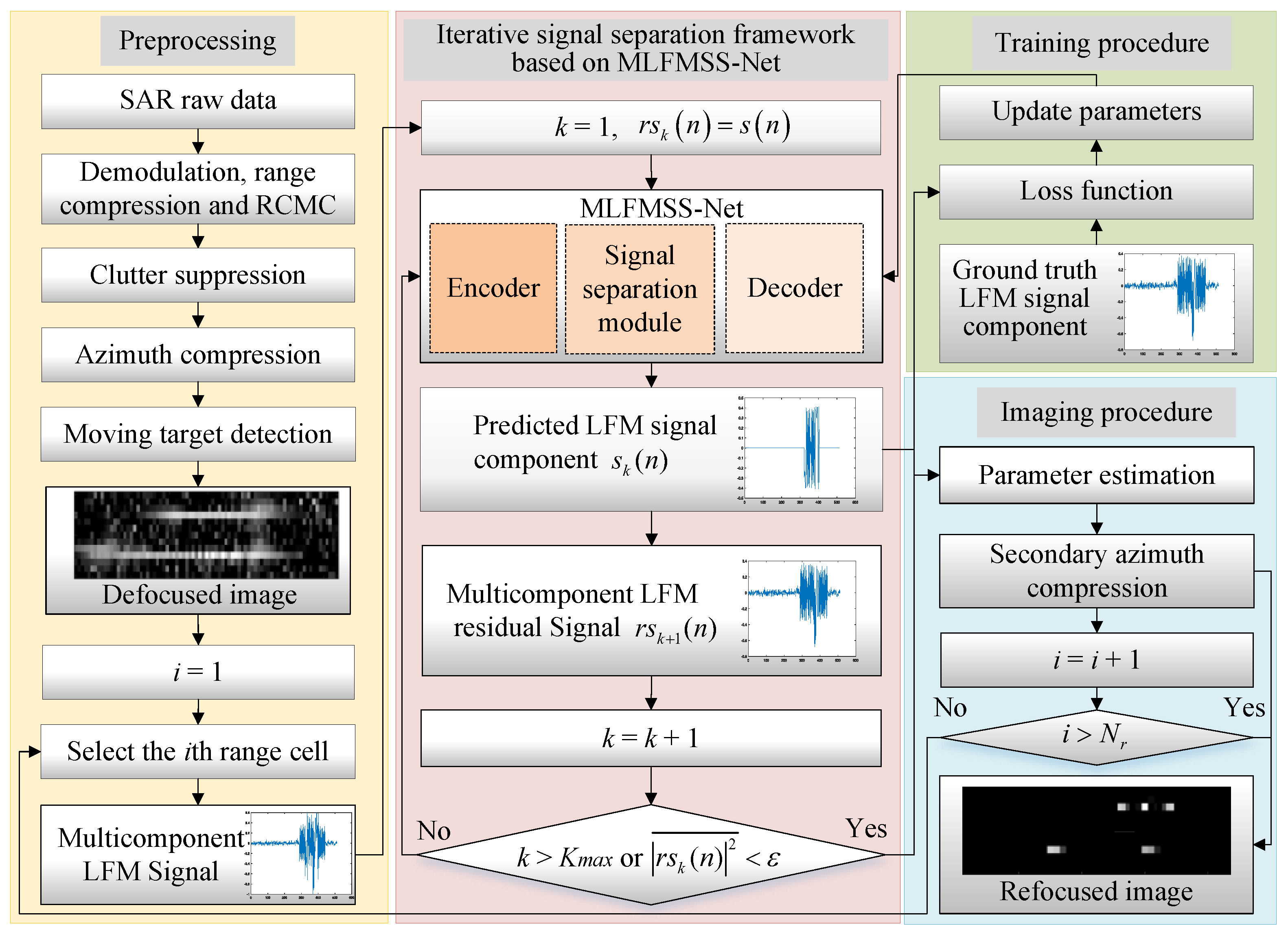
The flowchart of the proposed MLFMSS-Net-assisted multi-moving-target-imaging method is illustrated in Figure 2. In the preprocessing procedure, basic SAR imaging processing (including demodulation, range compression, RCMC, and azimuth compression) and clutter suppression are performed on the SAR raw data. Then, a constant false alarm rate (CFAR) detector is utilized to detect and extract the defocused moving-target image, each range cell of which can be modeled as a multicomponent LFM signal form given by Equation (13). Considering that different motion parameters of targets lead to different values of $a^k$ in Equation (13), it is difficult to directly perform the parameter estimation and the azimuth compression matched to each target parameter on $s\left(n\right)$. Therefore, the multicomponent LFM signal separation during the residual clutter elimination, i.e., $s\left(n\right)$ separation into $s_k\left(n\right),k=1,\dots ,K$ and $c{n}_{12}\left(n\right)$ elimination from $s\left(n\right)$, is a critical step for the multi-moving-target imaging before the parameter estimation and secondary azimuth compression. However, the unknown target numbers pose significant challenges for the signal-separation task. To address this problem, an iterative signal-separation framework based on a deep CNN is proposed. In this framework, a network named MLFMSS-Net is designed to extract the most-energetic LFM signal component from the multicomponent LFM signal, iteratively applied multiple times until all LFM signal components are successfully separated.

The most-energetic LFM signal-component-extraction task can be formulated as a regression problem, i.e.,  $s_k\left(n\right)=f_{\varphi }\left(s\left(n\right)\right)$, which can be solved by MLFMSS-Net. $f_{\varphi }\left(·\right)$ is the network with parameters $\varphi$. Utilizing a set of training data, MLFMSS-Net is trained through the minimization of the loss function. This training process enables the determination of optimal network parameters $\varphi$, leading to improved performance of the model. The network details will be discussed in subsequent subsections. Then, the well-trained MLFMSS-Net is applied in the iterative signal-separation framework. Specifically, the number of iterations and the residual are first initialized by $k=1$ and $r{s}_k\left(n\right)=s\left(n\right)$, respectively. At each iterative step, the well-trained MLFMSS-Net is employed to $r{s}_k\left(n\right)$ for the most-energetic LFM signal component $s_k\left(n\right)$ extraction. Then, the new signal component $s_k\left(n\right)$ is eliminated from $r{s}_k\left(n\right)$ to obtain the updated residual as follows:

$$r{s}_{k+1}\left(n\right)=r{s}_k\left(n\right)-s_k\left(n\right)=s\left(n\right)-\sum _{j=1}^{j=k}{s}_j\left(n\right)$$

(14)

The number of iterations is updated by $k\leftarrow k+1$. The aforementioned steps are repeated to extract a new LFM signal component from the residual $r{s}_k\left(n\right)$ until k either exceeds the maximum number $K_{max}$ of moving targets or the average power of the residual $\parallel r{s}_k\left(n\right){\parallel }_2^2$ is less than an empirical threshold value $\epsilon$. Given that $\epsilon$ is feasible for a new LFM signal component declaration, it is advisable to set the value of $\epsilon$ equal to the average power of the background clutter surrounding the moving targets for the residual clutter suppression. Then, let the target number $K\leftarrow k-1$. As a consequence, all LFM signal components’, $s_k\left(n\right),k=1,\dots ,K$, separation and residual clutter $c{n}_{12}\left(n\right)$ suppression from $s\left(n\right)$ have been achieved based on the proposed framework.

To realize K-moving-target imaging, in the imaging procedure, WVD is applied for the quadratic coefficient ${\widehat{a}}^k$ estimation of $s_k\left(n\right)$. Secondary azimuth compression matched to ${\widehat{a}}^k$ is further performed on the corresponding signal component $s_k\left(n\right)$ to generate the well-focused kth moving-target image as follows:

$$s_{ok}\left(n\right)={\mathcal{F}}^{-1}\left\{\mathcal{F}\left[s_k\left(n\right)\right]·\mathcal{F}\left[s_a\left(n\right)\right]\right\}$$

(15)

where $\mathcal{F}\left(·\right)$ and ${\mathcal{F}}^{-1}\left(·\right)$ denote the Fourier transform and the inverse Fourier transform, respectively. The azimuth matching function is expressed as $s_a\left(n\right)=\mathrm{rect}\left(n\right)exp\left(-j\pi {\widehat{a}}^k{n}^2\right)$. The azimuth multi-moving-target image of each range cell can be generated by the linear superposition of each target image as follows:

$$s_o\left(n\right)=\sum _{k=1}^{k=K}{s}_{ok}\left(n\right)$$

(16)

Therefore, the iterative signal-separation framework based on MLFMSS-Net, as well as the imaging procedure are implemented on each of the range cell data containing multiple targets to obtain the whole well-refocused moving-target image. The specific implementation procedures of the proposed method can be summarized in Algorithm 1.

Algorithm 1: The MLFMSS-Net-assisted multi-moving-target-imaging method

1  Preprocessing: Implement the basic SAR imaging processing and clutter suppression to obtain the defocused image of multiple moving targets 2  Input: Defocused multi-moving-target image 3  Output: Refocused multi-moving-target image 4  for $i\leftarrow 1$ to $N_r$ do 5     select the signal $s\left(n\right)$ from the ith range cell; 6     initialize $k\leftarrow 1$ and $r{s}_k\left(n\right)\leftarrow s\left(n\right)$; 7     while $k\le K_{max}$ or $\parallel r{s}_k\left(n\right){\parallel }_2^2\ge \epsilon$ do 8     $s_k\left(n\right)\leftarrow f_{\varphi }\left(s\left(n\right)\right)$ by the well-trained MLFMSS-Net;    /* design MLFMSS-Net $f_{\varphi }$, where the network parameters $\varphi$ are      optimized by minimizing the loss function through the      training data                                               */ 9     $r{s}_{k+1}\left(n\right)\leftarrow r{s}_k\left(n\right)-s_k\left(n\right)$; 10       $k\leftarrow k+1$; 11     end 12     $K\leftarrow k-1$; 13     for $k\leftarrow 1$ to K do 14     estimate ${\widehat{a}}^k$ of $s_k\left(n\right)$ by WVD; 15     $s_{ok}\left(n\right)\leftarrow {\mathcal{F}}^{-1}\left\{\mathcal{F}\left[s_k\left(n\right)\right]·\mathcal{F}\left[s_a\left(n\right)\right]\right\}$; 16     end 17     $s_o\left(n\right)\leftarrow {\sum }_{k=1}^{k=K}{s}_{ok}\left(n\right)$; 18  end

3.2. Dataset Description

Data pairs consisting of the multicomponent LFM signal and the corresponding most-energetic LFM signal component are required for the training of MLFMSS-Net. The multicomponent LFM signal from different SAR systems can be simulated according to Equation (13). It is worth mentioning that this network primarily focuses on refocusing the moving targets, rather than imaging the SAR observation scene. If all the large-sized SAR data are directly utilized as the network input, it would require a large amount of memory and computation time for training. Moreover, many clutter areas without moving targets are not useless for training. Instead of all the SAR data, therefore, numerous small-sized data patches with the length $N=512$ containing moving targets should be extracted from the SAR data and processed by the proposed MLFMSS-Net-assisted imaging method. The number of LFM signal components is a random integer from 0 to 5 for each signal sample. The signal parameters, respectively, obey the following uniform distributions: $|A^k|\sim U\left(0,1\right)$, $\mathsf{\Delta }{n}^k\sim U\left(0,N\right)$, $n_{ac}^k\sim U\left(0,N\right)$, $\mathsf{\Delta }{N}_a^k\sim U\left(0,N\right)$. Given that the SAR system parameters are implicitly embedded within the $a^k$ of $s\left(n\right)$, $a^k$ follows a uniform distribution over the reasonable range $U\left(-0.05,0.05\right)$. This ensures that the dataset contains multicomponent LFM signals from various SAR systems.

Because of the terrain’s heterogeneity, according to the analysis in [34], the additive perturbation $c{n}_{12}\left(n\right)$ was simulated under the assumption of a compound clutter model. This model accounts for heterogeneity in the data by assuming that each sampling cell is the product of a speckle random variable (RV) $\overline{X}$ and a statistically independent texture RV $\mathsf{\Delta }\in \left[0,\infty \right)$, i.e., $Y=\mathsf{\Delta }\times \overline{X}$. $\overline{X}$ is characterized by a complex Gaussian distribution ${\mathcal{N}}^{\mathbb{C}}\left(0,\left(1-\rho \right)\left({\sigma }_c^2+{\sigma }_n^2\right)\right)$, where $\rho$ is the correlation coefficient between two channels. ${\sigma }_c^2$ and ${\sigma }_c^2$ are the clutter and noise powers, respectively. It is convenient to normalize $\overline{X}$ to its expectation, i.e., $X=\overline{X}/\left(\left(1-\rho \right)\left({\sigma }_c^2+{\sigma }_n^2\right)\right)$. $\mathsf{\Delta }$ can be physically interpreted as the fluctuating variance (power) of the speckle. It is independent of the radar position and depends on the spatial distribution, orientation, and type of clutter under measurement. $\mathsf{\Delta }$ obeys the following distribution [34]:

$$f_{\mathsf{\Delta }}\left(\delta \right)=\frac{2{\left(\nu -1\right)}^{\nu }}{\mathsf{\Gamma }\left(\nu \right)}{\delta }^{-\left(2\nu +1\right)}exp\left(\frac{\left(1-\nu \right)}{{\delta }^2}\right)$$

(17)

where $\nu$ represents the texture parameter indicating the level of clutter heterogeneity in the imaging scene. A higher value of $\nu$ suggests a more-homogeneous scene, while a lower value indicates a more-heterogeneous scene. The density function of $c{n}_{12}\left(n\right)$ can be calculated by Bayes rule as follows [35]:

$$f_Y\left(y;\nu \right)=\frac{\mathsf{\Gamma }\left(\nu +1\right)}{\pi \mathsf{\Gamma }\left(\nu \right)}\frac{{\left(\nu -1\right)}^{\nu }}{{\left({\left|y\right|}^2+\nu -1\right)}^{\left(\nu +1\right)}}$$

(18)

According to the aforementioned distribution, $c{n}_{12}\left(n\right)$ can be simulated with a given $\nu$. To obtain the dataset containing the clutter with various heterogeneity levels, $\nu$ should follow the uniform distribution $\nu \sim U\left(3,50\right)$. Consequently, the multicomponent LFM signal can be obtained by summing the LFM signal components and the additive perturbation with different input SCNRs obeying the uniform distribution $U\left(-5\mathrm{dB},15\mathrm{dB}\right)$ in the dataset. The real and imaginary parts of the multicomponent LFM signal are divided into two independent channels as the network input $\mathit{I}\in {\mathbb{R}}^{N\times 2}$.

In addition, the most-energetic LFM signal component in the multicomponent LFM signal will be adopted as the output of MLFMSS-Net. Similarly, the real and imaginary parts of the signal component are treated as two independent channels, i.e., $\mathit{O}\in {\mathbb{R}}^{N\times 2}$.

Therefore, thousands of data pairs with diverse SAR system parameters, target motion characteristics, and clutter types have been generated for training and testing. It is worth noting that the minimax normalization strategy is utilized to normalize the dataset into the range [0, 1] for better network training and performance optimization.

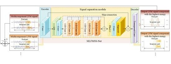
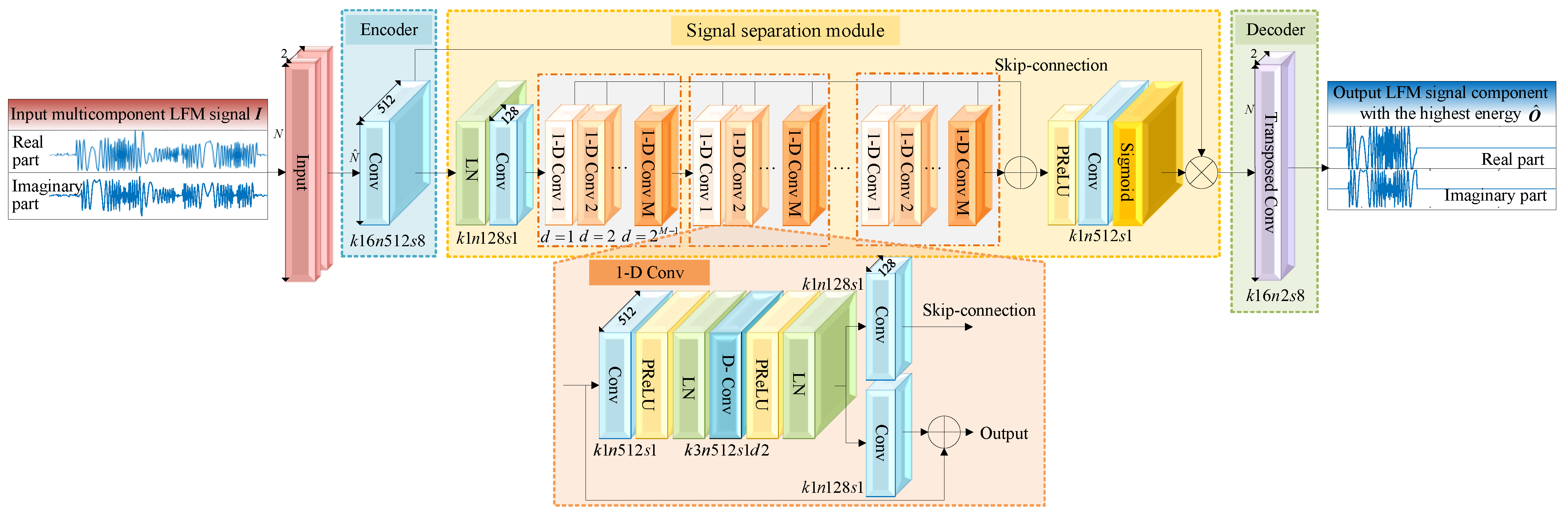
3.3. Architecture of Multicomponent Linear Frequency Modulation Signal-Separation-Net

As shown in Figure 3, MLFMSS-Net consists of the encoder, the signal-separation module, and the decoder. The notation $k16n32s8$ represents a 1D convolutional layer with a kernel size of 16, a filter number of 32, and a stride of 8. A convolutional layer without zero padding is utilized as the encoder to transform short segments of the network input $\mathit{I}\in {\mathbb{R}}^{N\times 2}$ into their corresponding representations $\mathit{F}\in {\mathbb{R}}^{\widehat{N}\times 512}$ in an intermediate feature space. The signal-separation module is then implemented by estimating a weighting function (mask) $\mathit{M}\in {\mathbb{R}}^{\widehat{N}\times 512}$, which is elementwise multiplied with the encoder output, i.e., $\mathit{S}=\mathit{M}\odot \mathit{F}$, where ⊙ denotes the elementwise multiplication. Finally, a transposed convolutional layer as the decoder is exploited to transform the masked encoder feature into the LFM signal component with the highest energy $\widehat{\mathit{O}}\in {\mathbb{R}}^{N\times 2}$. We describe the details of the signal-separation module in the following.

3.3.1. Signal-Separation Module

For the separation mask $\mathit{M}$ estimation, the global layer normalization (gLN) is first exploited to normalize the feature over both the channel and time dimensions [36]. A convolutional layer of kernel size 1 is added as a bottleneck layer to adaptively fuse the effective features and stabilize the training of the deeper network. Inspired by the network for audio separation, the mask can be generated by a temporal convolutional network (TCN) [26,37]. This TCN is composed of multiple 1D dilated convolutional blocks (1D Convs), which enable the network to capture long-term dependencies within the input signal while maintaining a compact model size. The 1D Conv with an exponentially increasing dilation factor ensures a sufficiently large temporal context window to take advantage of the long-range dependencies of the signal. In the signal-separation module, eight 1D Convs with dilation factors $d=1,2,\dots ,2^7$ are repeated 3 times. A residual path and a skip-connection path of each 1D Conv are applied: the residual path of the current 1D Conv is directly fed into the next block, while the skip-connection paths for all blocks are summed up and utilized as the output of the TCN, which is passed to a parametric rectified linear unit (PReLU) activation function [38]. Finally, a convolutional layer with a Sigmoid function is applied to estimate the mask.

3.3.2. One-Dimensional Dilated Convolutional Block

In each 1D Conv, as shown in Figure 3, a convolutional layer with a kernel size of 1 is first added to increase the complexity and richness of the features. The PReLU activation function is utilized to introduce nonlinearity and is followed by a gLN. Subsequently, to further reduce the number of parameters while maintaining a certain level of feature representation capability, the depthwise separable convolution can be employed as a substitute for the standard convolutional operation [39]. The depthwise separable convolution operator decouples the standard convolution operation into a depthwise convolution (D-Conv) with dilation factor d and a pointwise convolution. Besides, a PReLU activation function together with a normalization operation is added after the D-Conv. Each 1D Conv consists of a residual path and a skip-connection path, which improve the flow of information and gradient throughout the network.

3.4. Training Procedure

To achieve the desired signal separation performance of MLFMSS-Net, the network is required to be trained by minimizing a signal separation loss, denoted as ${\mathcal{L}}_{sp}(\widehat{\mathit{O}},\mathit{O})$. Here, $\widehat{\mathit{O}}$ represents the predicted output of the network $f_{\varphi }\left(\mathit{I}\right)$ and $\mathit{O}$ is the ground truth LFM signal component with the highest energy. The signal-separation task can be formulated as a regression problem, where the goal is to minimize the difference between the predicted and ground truth signals. This is typically achieved by applying the pixelwise squared Euclidean distance as the loss function:

$${\mathcal{L}}_{sp}\left(\widehat{\mathit{O}},\mathit{O}\right)={\parallel \widehat{\mathit{O}}-\mathit{O}\parallel }_2^2$$

(19)

An NVIDIA GeForce GTX3090 GPU was utilized to train the MLFMSS-Net model. The model was trained with 500,000 training samples and 150,000 validation samples. Then, 150,000 samples were used for testing. The batch size was configured to 32 during the training process. Furthermore, Adam [40] was exploited as the optimization algorithm to update $\varphi$ at each step. The learning rate of the network was initially set to $5\times {10}^{-4}$ and decayed by 0.5 for every 5 epochs. This allowed the network to gradually adjust its parameters towards the optimal values that minimize the loss function.

During training, MLFMSS-Net underwent 125,000 backpropagation iterations within 1.46 h, resulting in a good fitting performance. The well-trained network is capable of achieving accurate predictions of outputs for unseen inputs. It has learned and captured the mapping relationship between its input and output, allowing it to generate the LFM signal component by simply calculating $\widehat{\mathit{O}}=f_{\varphi }\left(\mathit{I}\right)$.

4. Experimental Results and Performance Analysis

In this section, the signal separation performance of the trained MLFMSS-Net is analyzed by the multicomponent LFM signal simulation in Section 4.1. Moreover, the imaging results on both the simulated and real SAR data are further presented to verify the feasibility and effectiveness of the proposed MLFMSS-Net-assisted multi-moving-target-imaging method in Section 4.2 and Section 4.3.

4.1. Results on Simulated Multicomponent Linear Frequency Modulation Signal

In this subsection, the signal separation performance of the trained MLFMSS-Net is explored by a three-component LFM signal, the parameters of which are listed in

Table 1. Parameters of simulated three-component LFM signal.

Components	$|{\mathit{A}}^{\mathit{k}}|$	$\mathsf{\Delta }{\mathit{n}}^{\mathit{k}}$	${\mathit{n}}_{\mathbf{ac}}^{\mathit{k}}$	$\mathsf{\Delta }{\mathit{N}}_{\mathit{a}}^{\mathit{k}}$	${\mathit{a}}^{\mathit{k}}$
1	1	100	100	100	−0.008
2	0.8	100	200	80	0.01
3	0.5	50	0	100	0.002

. The additive perturbation with $\nu =5$ was added with the SCNR $=10 \mathrm{dB}$. The real and imaginary parts of the three-component LFM signal are shown in Figure 4a,b, respectively. The three LFM signal components overlap with each other and are contaminated by the additive perturbation, which makes the signal separation more challenging. Utilizing the iterative signal-separation framework based on MLFMSS-Net, the separation results of the three LFM signal components are given in Figure 4c–h. It can be seen that the separated signal components are similar to the ground truth signals. Therefore, MLFMSS-Net achieved a good signal separation performance.

The correlation coefficient between the ground truth and predicted signal components was utilized to numerically evaluate the separation accuracy in various SCNR scenarios as follows:

$$\rho =\frac{{\displaystyle \sum _{i=1}^N}\left|\widehat{\mathit{O}}\left(i\right){\mathit{O}}^{*}\left(i\right)\right|}{\sqrt{{\displaystyle \sum _{i=1}^N}{\left|\widehat{\mathit{O}}\left(i\right)\right|}^2{\displaystyle \sum _{i=1}^N}{\left|{\mathit{O}}^{*}\left(i\right)\right|}^2}}.$$

(20)

where ${\mathit{O}}^{*}$ is the conjugate of $\mathit{O}$. The correlation between the two signals becomes stronger as the value of $\rho$ approaches 1. A total of 500 trials were conducted for each input SCNR within the range [−5 dB, 10 dB]. The Chirplet decomposition method [10,11] was utilized to compare the separation accuracy of MLFMSS-Net.

As depicted in Figure 5, the correlation coefficient rose as the SCNR increased. Compared with Chirplet decomposition, it was evident that MLFMSS-Net exhibited superior accuracy in signal separation. Notably, when the SCNR exceeded 0 dB, MLFMSS-Net achieved a correlation coefficient exceeding 95%. This is because MLFMSS-Net was trained by minimizing the squared Euclidean distance, i.e., $min\parallel f_{\varphi }\left(\mathit{I}\right){-\mathit{O}\parallel }_2^2$. Once this training process was complete, the optimal parameters $\varphi$ could be obtained. The trained MLFMSS-Net was capable of generating the predicted signal component $\widehat{\mathit{O}}=f_{\varphi }\left(\mathit{I}\right)$ that had the minimum difference from the ground truth signal component $\mathit{O}$.

4.2. Results on Simulated SAR Data

To effectively analyze the imaging quality of the proposed MLFMSS-Net-assisted method in different SAR systems, two relatively complicated imaging scenarios were simulated in airborne and spaceborne SAR systems for testing, respectively. The parameters of the airborne and spaceborne SAR systems are listed in

Table 2. Parameters of airborne SAR system.

Parameter	Notation	Value
Wavelength	$\lambda$	0.03 m
Platform velocity	V	150 m/s
Pulse repetition frequency	PRF	800 Hz
Slant range	$R_B$	10 km

and

Table 3. Parameters of spaceborne SAR system.

Parameter	Notation	Value
Wavelength	$\lambda$	0.03 m
Platform velocity	V	7068 m/s
Pulse repetition frequency	PRF	4560 Hz
Slant range	$R_B$	700 km

, respectively.

The first scenario containing four moving point targets and the additive perturbation with the input SCNR $=5 \mathrm{dB}$ was simulated in the airborne SAR system, as shown in Figure 6a. It can be observed that the responses of moving targets are defocused in azimuth and overlap with each other in the SAR image. Chirplet decomposition [10,11] was utilized to separate the multi-moving-target signal and estimate the corresponding Doppler chirp rate. The refocused target image can be obtained by the secondary azimuth compression matched to the estimated Doppler chirp rate. As shown in Figure 6b, all targets are refocused in azimuth with some residual clutter around them. In Figure 6c, the well-refocused SAR image can be generated by the proposed MLFMSS-Net-based imaging method. Moreover, it provided better residual clutter suppression performance than Chirplet decomposition. Besides, the correlation coefficients of targets MT2-MT4 with different methods are observed in Figure 7. It can be seen that MLFMSS-Net achieved better separation accuracy than Chirplet decomposition, especially in the low SCNR case.

Furthermore, another scenario with the input SCNR $=0 \mathrm{dB}$ in the spaceborne SAR system is simulated in Figure 8a. The imaging results based on Chirplet decomposition and MLFMSS-Net are, respectively, depicted in Figure 8b,c. The moving-target image obtained by the Chirplet-decomposition-based imaging method is submerged in the strong background clutter, which brings difficulty to target detection. In comparison, the MLFMSS-Net-based imaging method realizes image focusing and residual clutter suppression in a strong clutter environment. Therefore, the proposed MLFMSS-Net-based imaging method is capable of achieving multi-moving-target imaging with different radar system parameters, moving target characteristics, and clutter types.

The image focusing performance of the proposed method was quantitatively evaluated by the image entropy [41], with smaller values indicating better focus and clarity. In addition, the output SCNR was utilized to numerically measure the clutter suppression performance. As listed in

Table 4. Imaging quality for simulated SAR data.

Platform	Metric	Original	Chirplet	MLFMSS-Net
Airborne	Entropy	9.849	6.682	4.200
	SCNR (dB)	5.000	31.46	41.07
Spaceborne	Entropy	9.859	8.249	5.095
	SCNR (dB)	0.000	18.29	38.42

for the two scenarios, the imaging quality of the Chirplet-decomposition-based imaging method is greatly enhanced compared with the original image. The MLFMSS-Net-based imaging method achieves the best image focusing and clutter suppression performance, which further verifies the effectiveness of the proposed method. In addition, MLFMSS-Net costs a much shorter running time of 6.876 s compared with the 273.6 s required by Chirplet decomposition. Therefore, the proposed imaging method based on MLFMSS-Net achieves great improvements in both imaging quality and efficiency.

4.3. Results on Real SAR Data

In this subsection, real airborne SAR data and satellite TerraSAR-X data are both utilized to further demonstrate the effectiveness of the proposed imaging method. The parameters of the two SAR systems were the same as those of the simulations, as listed in Table 2 and Table 3. Figure 9a shows the original image containing six moving targets MT1-MT6 in the airborne SAR system. All moving targets are defocused owing to the target motion and obscured by the background clutter. MT3-MT6 are close in distance and overlap with each other, making it difficult to distinguish them. The imaging results based on Chirplet decomposition and MLFMSS-Net are shown in Figure 9b,c, respectively. Six moving targets can be well refocused, making them easy to distinguish. Compared with Chirplet decomposition, the MLFMSS-Net-based imaging method obtains few virtual targets and provides superior imaging performance in azimuth.

Moreover, the imaging results of TerraSAR-X data containing three moving targets were obtained as shown in Figure 10. As shown in Figure 10b,c, the moving targets are well refocused while the background residual clutter is suppressed based on Chirplet decomposition and MLFMSS-Net. The entropy and SCNR for TerraSAR-X data are listed in

Table 5. Imaging quality for real SAR data.

Platform	Metric	Original	Chirplet	MLFMSS-Net
Airborne	Entropy	9.233	6.333	5.570
	SCNR (dB)	−0.671	29.28	34.88
TerraSAR-X	Entropy	8.418	4.867	4.485
	SCNR (dB)	5.036	31.20	47.83

. Compared with other methods, the imaging method based on MLFMSS-Net has lower image entropy and a larger SCNR, which achieves better refocusing and clutter suppression performance.

5. Discussion

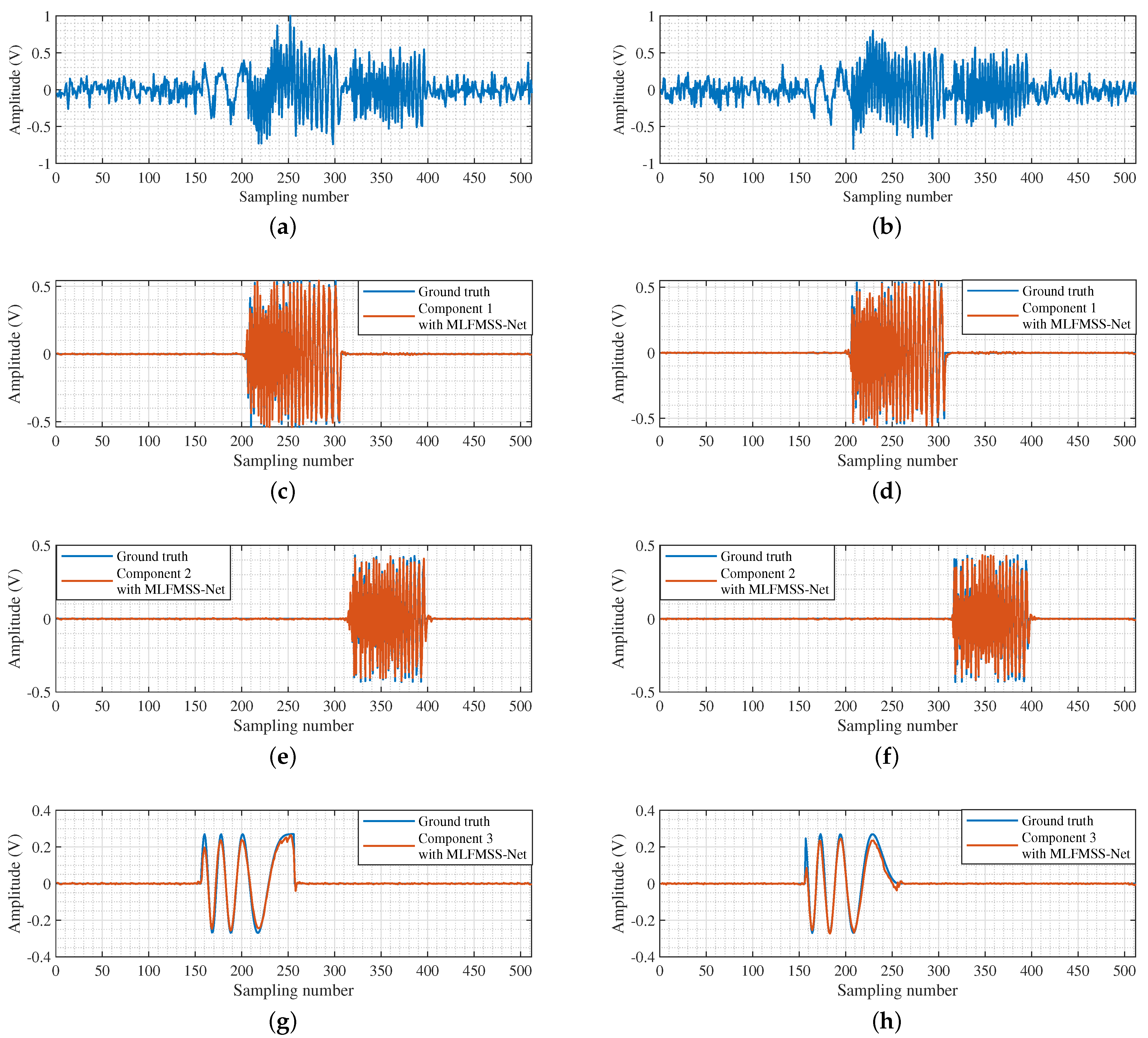
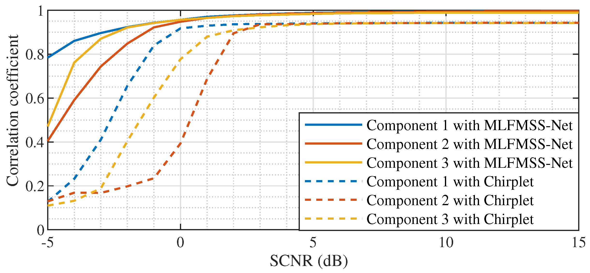
In Section 4.2, two simulated data acquired by the airborne and spaceborne SAR systems were both utilized to verify the applicability of the proposed imaging method. The results showed that the trained MLFMSS-Net realizes the separation of multicomponent LFM signals from different SAR systems. With the assistance of MLFMSS-Net, the proposed imaging method achieves high-quality and high-efficiency imaging without prior knowledge of the system parameters. The reason behind this success lies in the fact that the training dataset was generated based on a multicomponent LFM signal model, the parameters of which implicitly embed the radar system parameter information. By training MLFMSS-Net on this abundant dataset containing different signal parameters, the network becomes adaptable to various radar systems. In Section 4.3, experiments on two sets of real data acquired from airborne SAR systems and the TerraSAR-X satellite further confirmed the ability of the proposed method to improve the robustness of moving-target imaging, while reducing sensitivity to the system parameters. This is of great significance for the application of the proposed method in real-world scenarios.

Meanwhile, experiments with different target numbers in Section 4 demonstrated that the proposed method is capable of achieving the multi-moving-target imaging without prior knowledge of the target number, exhibiting its suitability for practical imaging scenarios.

However, it is worthwhile to remark that the length of the separated signals in the experiments was fixed owing to the fixed training sample length in the dataset, limiting the flexibility of moving-target imaging processing. Therefore, our future work will focus on how to improve the adaptability of the network model to the separated signals with different lengths, such as more-diverse data sample generation and multi-scale model building.

6. Conclusions

In this paper, we propose a MLFMSS-Net-assisted multi-moving-target-imaging method for the SAR-GMTI system. The network MLFMSS-Net was designed to extract the most-energetic LFM signal component from the multicomponent LFM signal and trained on the dataset with various SAR system parameters, target information, and clutter types, which was generated by the multicomponent LFM signal model. The well-trained MLFMSS-Net was iteratively applied multiple times to realize all LFM signal component separation and residual clutter suppression. Without prior knowledge of the target number, compared with other methods, the target imaging and residual clutter suppression performance were improved with high processing efficiency, especially in low-input SCNR scenarios. It provides further potential to implement the subsequent image interpretation including target classification and recognition. Meanwhile, the proposed method enhances the robustness of moving-target imaging, while reducing sensitivity to the system parameters, preliminarily addressing a significant challenge faced by deep-learning-based imaging methods. This allows the deep-learning-based imaging method to be a suitable solution for practical imaging applications.

In future work, we will further investigate how to incorporate the parameter estimation and pulse compression tasks into the deep network, aiming to overcome the limitations of the inherent resolution on estimation accuracy for traditional TFR-based methods and the signal bandwidth on imaging resolution for matched filtering methods. Additionally, the proposed method focuses on the imaging of ground moving targets with accelerated motions, the radar echoes of which can be characterized as the multicomponent LFM signal model. However, this signal model and the corresponding imaging method are not suitable for maritime targets with complex motions. A multicomponent higher-order phase signal model needs to be established. Subsequent research will explore how to fully utilize the powerful feature extraction and signal separation capabilities of MLFMSS-Net and generalize its applications to complex signal models.