

Assessment and Prediction of Sea Level and Coastal Wetland Changes in Small Islands Using Remote Sensing and Artificial Intelligence


Abstract
1. Introduction
2. Materials and Methods
2.1. Data Preprocessing, Partitioning and Normalisation
2.2. Sea Level Prediction
2.2.1. Multilinear Regression
2.2.2. Random Forest Model
2.2.3. Multi-Layer Perceptron
2.2.4. Bidirectional Long Short-Term Memory
2.3. Model Evaluation
- Correlation coefficient (r)
- 2.
- Willmott’s Index of Agreement (d)
- 3.
- Legates and McCabe’s Index (LM)
- 4.
- Root mean square error (RMSE)
- 5.
- Mean absolute error (MAE)
2.4. Wetland and Mangrove Detection
3. Results
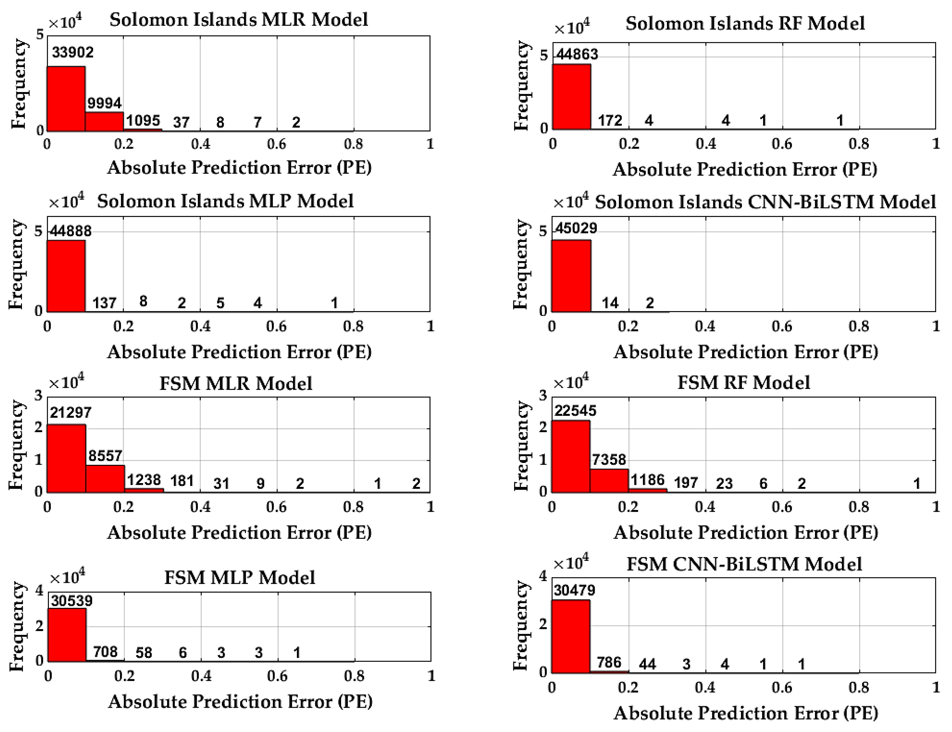
3.1. Model Performance Metrics for Sea Level Prediction Using Machine Learning
3.2. Classification of Wetlands
4. Discussion
4.1. Prediction of Sea Level Trends
4.2. Detection of Wetland Change
5. Conclusions
Author Contributions
Funding
Data Availability Statement
Conflicts of Interest
Appendix A

| Solomon Islands | Federated States of Micronesia | |||||
|---|---|---|---|---|---|---|
| Annual MSL (m above TG Zero) | Total (Guadalcanal) Mangrove Area (km2) | National (Guadalcanal) Coastline Coverage (km) | Annual MSL (m above TG Zero) | Total (Pohnpei) Mangrove Area (km2) | National (Pohnpei) Coastline Coverage (km) | |
| 1994 | 0.5403 | |||||
| 1995 | 0.6377 | |||||
| 1996 | 0.7129 | 527.31 (11.67) | 4371.56 (84.44) | 90.84 (56.69) | 402.71 (204.95) | |
| 1997 | 0.5650 | |||||
| 1998 | 0.4962 | |||||
| 1999 | 0.7309 | |||||
| 2000 | 0.7589 | |||||
| 2001 | 0.7112 | 0.5900 | ||||
| 2002 | 0.6356 | 0.7131 | ||||
| 2003 | 0.6563 | 0.7199 | ||||
| 2004 | 0.6528 | 0.7279 | ||||
| 2005 | 0.6710 | 0.7345 | ||||
| 2006 | 0.7204 | 0.7266 | ||||
| 2007 | 0.7151 | 529.25 (11.63) | 4359.06 (84.25) | 0.8220 | 88.18 (54.61) | 399.6 (203.11) |
| 2008 | 0.7307 | 530.04 (11.62) | 4357.74 (84.95) | 0.8012 | 88.01 (54.61) | 399.05 (203.11) |
| 2009 | 0.7253 | 530.84 (11.71) | 4352.74 (84.91) | 0.7616 | 87.91 (54.51) | 397.65 (202.36) |
| 2010 | 0.6684 | 528.98 (11.77) | 4348.12 (84.82) | 0.8169 | 90.17 (56.56) | 400.91 (204.86) |
| 2011 | 0.8024 | 0.8455 | ||||
| 2012 | 0.7783 | 0.8585 | ||||
| 2013 | 0.7337 | 0.8251 | ||||
| 2014 | 0.7191 | 0.7431 | ||||
| 2015 | 0.6536 | 525.48 | 4339.18 (84.85) | 0.5936 | 90.69 | 402.17 (204.86) |
| 2016 | 0.6164 | 523.58 | 4337.32 (84.91) | 0.8090 | 90.69 | 402.17 (204.86) |
| 2017 | 0.7517 | 522.21 | 4330.31 (84.91) | 0.8387 | 90.69 | 402.17 (204.86) |
| 2018 | 0.7663 | 524.71 | 4332 (84.88) | 0.7727 | 90.69 | 402.17 (204.86) |
| 2019 | 0.7022 | 527.5 | 4343.49 (84.25) | 0.7961 | 88.18 | 398.59 (202.39) |
| 2020 | 0.7582 | 526.51 | 4346.61 (83.44) | 0.8447 | 87.94 | 398.49 (202.51) |
| 2021 | 0.8429 | 0.8619 | ||||
| 2022 | 0.8950 | 0.9093 | ||||
References
- Monnereau, I.; Abraham, S. Limits to Autonomous Adaptation in Response to Coastal Erosion in Kosrae, Micronesia. Int. J. Glob. Warm. 2013, 5, 416–432. [Google Scholar] [CrossRef]
- Ha’apio, M.O.; Morrison, K.; Gonzalez, R.; Wairiu, M.; Holland, E. Limits and Barriers to Transformation: A Case Study of April Ridge Relocation Initiative, East Honiara, Solomon Islands. In Climate Change Impacts and Adaptation Strategies for Coastal Communities; Climate Change Management Book Series; Springer: Berlin/Heidelberg, Germany, 2018; pp. 455–470. [Google Scholar] [CrossRef]
- Boero, F.; Treguier, A.M.; Philippart, C.; Huse, G.; Gault, J.; Schneider, R.; Cummins, V.; Garcia-Soto, C.; Patterson, D.; Lacroix, D.; et al. Navigating the Future V: Marine Science for a Sustainable Future. Zenodo 2019. [Google Scholar] [CrossRef]
- Timmermann, A.; McGregor, S.; Jin, F.-F. Wind Effects on Past and Future Regional Sea Level Trends in the Southern Indo-Pacific. J. Clim. 2010, 23, 4429–4437. [Google Scholar] [CrossRef]
- Isiaka, I.; Ndukwe, K.; Chibuike, U. Mean Sea Level: The Effect of the Rise in the Environment. J. Geoinform. Environ. Res. 2021, 2, 92–102. [Google Scholar] [CrossRef]
- Albert, S.; Bronen, R.; Tooler, N.; Leon, J.; Yee, D.; Ash, J.; Boseto, D.; Grinham, A. Heading for the Hills: Climate-Driven Community Relocations in the Solomon Islands and Alaska Provide Insight for a 1.5 °C Future. Reg. Environ. Change 2018, 18, 2261–2272. [Google Scholar] [CrossRef]
- IPCC. Climate Change 2022: Impacts, Adaptation and Vulnerability; Cambridge University Press: Cambridge, UK, 2022. [Google Scholar] [CrossRef]
- Church, J.A.; White, N.J.; Hunter, J.R. Sea-Level Rise at Tropical Pacific and Indian Ocean Islands. Glob. Planet. Change 2006, 53, 155–168. [Google Scholar] [CrossRef]
- Klein, A. Eight Low-Lying Pacific Islands Swallowed Whole by Rising Seas. Available online: https://www.newscientist.com/article/2146594-eight-low-lying-pacific-islands-swallowed-whole-by-rising-seas/ (accessed on 16 March 2023).
- Mcleod, E.; Hinkel, J.; Vafeidis, A.T.; Nicholls, R.J.; Harvey, N.; Salm, R. Sea-Level Rise Vulnerability in the Countries of the Coral Triangle. Sustain. Sci. 2010, 5, 207–222. [Google Scholar] [CrossRef]
- André, L.V.; Van Wynsberge, S.; Chinain, M.; Andréfouët, S. An Appraisal of Systematic Conservation Planning for Pacific Ocean Tropical Islands Coastal Environments. Mar. Pollut. Bull. 2021, 165, 1121131. [Google Scholar] [CrossRef] [PubMed]
- Gilman, E.; Van Lavieren, H.; Ellison, J.; Jungblut, V.; Wilson, L.; Areki, F.; Brighouse, G.; Bungitak, J.; Dus, E.; Kilman, M.; et al. Pacific Island Mangroves in a Changing Climate and Rising Sea; Regional Seas; United Nations Environment Programme: Nairobi, Kenya, 2006; ISBN 978-92-807-2741-8. [Google Scholar]
- Raj, N.; Gharineiat, Z.; Ahmed, A.A.M.; Stepanyants, Y. Assessment and Prediction of Sea Level Trend in the South Pacific Region. Remote Sens. 2022, 14, 986. [Google Scholar] [CrossRef]
- Tiggeloven, T.; Couasnon, A.; van Straaten, C.; Muis, S.; Ward, P.J. Exploring Deep Learning Capabilities for Surge Predictions in Coastal Areas. Sci. Rep. 2021, 11, 17224. [Google Scholar] [CrossRef] [PubMed]
- Raj, N. Prediction of Sea Level with Vertical Land Movement Correction Using Deep Learning. Mathematics 2022, 10, 4533. [Google Scholar] [CrossRef]
- Raj, N.; Brown, J. An EEMD-BiLSTM Algorithm Integrated with Boruta Random Forest Optimiser for Significant Wave Height Forecasting along Coastal Areas of Queensland, Australia. Remote Sens. 2021, 13, 1456. [Google Scholar] [CrossRef]
- Moishin, M.; Deo, R.C.; Prasad, R.; Raj, N.; Abdulla, S. Designing Deep-Based Learning Flood Forecast Model with ConvLSTM Hybrid Algorithm. IEEE Access 2021, 9, 50982–50993. [Google Scholar] [CrossRef]
- Sharma, E.; Deo, R.C.; Prasad, R.; Parisi, A.V.; Raj, N. Deep Air Quality Forecasts: Suspended Particulate Matter Modeling with Convolutional Neural and Long Short-Term Memory Networks. IEEE Access 2020, 8, 209503–209516. [Google Scholar] [CrossRef]
- Berryman, A.; Turchin, P. Identifying the Density—Dependent Structure Underlying Ecological Time Series. Oikos 2001, 92, 265–270. [Google Scholar] [CrossRef]
- Nkoro, E.; Uko, A.K. Autoregressive Distributed Lag (ARDL) Cointegration Technique: Application and Interpretation. J. Stat. Econom. Methods 2016, 5, 63–91. [Google Scholar]
- Gaur, A.; Pachori, R.B.; Wang, H.; Prasad, G. An Automatic Subject Specific Intrinsic Mode Function Selection for Enhancing Two-Class EEG-Based Motor Imagery-Brain Computer Interface. IEEE Sens. 2019, 19, 6938–6947. [Google Scholar] [CrossRef]
- Ur Rehman, N.; Aftab, H. Multivariate Variational Mode Decomposition. IEEE Trans. Signal Process. 2019, 67, 6039–6052. [Google Scholar] [CrossRef]
- Alasadi, S.A.; Bhaya, W.S. Review of Data Preprocessing Techniques in Data Mining. J. Eng. Appl. Sci. 2017, 12, 4102–4107. [Google Scholar]
- Lou, R.; Lv, Z.; Dang, S.; Su, T.; Li, X. Application of Machine Learning in Ocean Data. In Multimedia Systems; Springer: Berlin/Heidelberg, Germany, 2021. [Google Scholar] [CrossRef]
- Atmaja, T.; Fukushi, K. Empowering Geo-Based AI Algorithm to Aid Coastal Flood Risk Analysis: A Review and Development Framework. ISPRS Ann. Photogramm. Remote Sens. Spatial Inf. Sci. 2022, V-3-2022, 517–523. [Google Scholar] [CrossRef]
- Rehman, S.; Sahana, M.; Hong, H.; Sajjad, H.; Ahmed, B.B. A Systematic Review on Approaches and Methods Used for Flood Vulnerability Assessment: Framework for Future Research. Nat. Hazards 2019, 96, 975–998. [Google Scholar] [CrossRef]
- Breiman, L. Random Forests. Mach. Learn. 2001, 45, 5–32. [Google Scholar] [CrossRef]
- Tahraoui, H.; Amrane, A.; Belhadj, A.-E.; Zhang, J. Modeling the Organic Matter of Water Using the Decision Tree Coupled with Bootstrap Aggregated and Least-Squares Boosting. Environ. Technol. Innov. 2022, 27, 102419. [Google Scholar] [CrossRef]
- Ahmed, A.; Deo, R.C.; Feng, Q.; Ghahramani, A.; Raj, N.; Yin, Z.; Yang, L. Hybrid Deep Learning Method for a Week-Ahead Evapotranspiration Forecasting. Stoch. Environ. Res. Risk Assess. 2022, 36, 831–849. [Google Scholar] [CrossRef]
- Hopp, D. Using Machine Learning to Make Government Spending Greener. Stat. J. IAOS 2022, 38, 1053–1065. [Google Scholar] [CrossRef]
- Latif, S.D.; Chong, K.L.; Ahmed, A.N.; Huang, Y.F.; Sherif, M.; El-Shafie, A. Sediment Load Prediction in Johor River: Deep Learning versus Machine Learning Models. Appl. Water Sci. 2023, 13, 79. [Google Scholar] [CrossRef]
- Bagheri, M.; Ibrahim, Z.Z.; Wolf, I.D.; Akhir, M.F.; Talaat, W.I.A.W.; Oryani, B. Sea-Level Projections Using a NARX-NN Model of Tide Gauge Data for the Coastal City of Kuala Terengganu in Malaysia. Environ. Sci. Pollut. Res. 2022, 30, 81839–81857. [Google Scholar] [CrossRef]
- Ahmed, A.; Deo, R.C.; Feng, Q.; Ghahramani, A.; Raj, N.; Yin, Z.; Yang, L. Deep Learning Hybrid Model with Boruta-Random Forest Optimiser Algorithm for Streamflow Forecasting with Climate Mode Indices, Rainfall, and Periodicity. J. Hydrol. 2021, 599, 126350. [Google Scholar] [CrossRef]
- Tran, T.T.; Pham, N.H.; Pham, Q.B.; Pham, T.L.; Ngo, X.Q.; Nguyen, D.L.; Nguyen, P.N.; Veettil, B.K. Performances of Different Machine Learning Algorithms for Predicting Saltwater Intrusion in the Vietnamese Mekong Delta Using Limited Input Data: A Study from Ham Luong River. Water Resour. 2022, 49, 391–401. [Google Scholar] [CrossRef]
- Hodson, T.O. Root-Mean-Square Error (RMSE) or Mean Absolute Error (MAE): When to Use Them or Not. Geosci. Model Dev. 2022, 15, 5481–5487. [Google Scholar] [CrossRef]
- Willmott, C.J.; Matsumura, K. Advantages of the Mean Absolute Error (MAE) Over the Root Mean Square Error (RMSE) in Assessing Average Model Performance. Clim. Res. 2005, 30, 79–82. [Google Scholar] [CrossRef]
- Shi, T.; Liu, J.; Hu, Z.; Wang, J.; Wu, G. New Spectral Metrics for Mangrove Forest Identification. Remote Sens. Lett. 2016, 7, 885–894. [Google Scholar] [CrossRef]
- Xu, H. Modification of Normalised Difference Water Index (NDWI) to Enhance Open Water Features in Remotely Sensed Imagery. Int. J. Remote Sens. 2006, 27, 3025–3033. [Google Scholar] [CrossRef]
- Melillos, G.; Hadjimitsis, D.G. Using Simple Ratio (SR) Vegetation Index to Detect Deep Man-Made Infrastructures in Cyprus. In Detection and Sensing of Mines, Explosive Objects, and Obscured Targets XXV; SPIE: Bellingham, WA, USA, 2020. [Google Scholar] [CrossRef]
- Jubeh, G.; Mimi, Z. Governance and Climate Vulnerability Index. Water Resour. Manag. 2012, 26, 4147–4162. [Google Scholar] [CrossRef]
- Islam, M.S.; Uddin, M.A.; Hossain, M.A. Assessing the Dynamics of Land Cover and Shoreline Changes of Nijhum Dwip (Island) of Bangladesh Using Remote Sensing and GIS Techniques. Reg. Stud. Mar. Sci. 2021, 41, 101578. [Google Scholar] [CrossRef]
- Samanta, S.; Hazra, S.; Mondal, P.P.; Chanda, A.; Giri, S.; French, J.R.; Nicholls, R.J. Assessment and Attribution of Mangrove Forest Changes in the Indian Sundarbans from 2000 to 2020. Remote Sens. 2021, 13, 4957. [Google Scholar] [CrossRef]
- Xiao, H.; Su, F.; Fu, D.; Wang, Q.; Huang, C. Coastal Mangrove Response to Marine Erosion: Evaluating the Impacts of Spatial Distribution and Vegetation Growth in Bangkok Bay from 1987 to 2017. Remote Sens. 2020, 12, 220. [Google Scholar] [CrossRef]
- da Costa Cavalcante, J.; de Lima, A.M.M.; da Silva, J.C.C.; de Holanda, B.S.; Almeida, C.A. Temporal Analysis of the Mangrove Forest at the Mocajuba River Hydrographic Basin-Pará. Floresta Ambient. 2021, 28, e20200073. [Google Scholar] [CrossRef]
- Mohanty, P.C.; Shetty, S.; Mahendra, R.S.; Nayak, R.K.; Sharma, L.K.; Rama Rao, E.P. Spatio-Temporal Changes of Mangrove Cover and Its Impact on Bio-Carbon Flux along the West Bengal Coast, Northeast Coast of India. Eur. J. Remote Sens. 2021, 54, 525–537. [Google Scholar] [CrossRef]
- Khedher, K.M.; Abu-Taweel, G.M.; Al-Fifi, Z.; Qoradi, M.D.; Al-khafaji, Z.; Halder, B.; Bandyopadhyay, J.; Shahid, S.; Essaied, L.; Yaseen, Z.M. Farasan Island of Saudi Arabia Confronts the Measurable Impacts of Global Warming in 45 Years. Sci. Rep. 2022, 12, 14322. [Google Scholar] [CrossRef] [PubMed]
- Woltz, V.L.; Peneva-Reed, E.I.; Zhu, Z.; Bullock, E.L.; MacKenzie, R.A.; Apwong, M.; Krauss, K.W.; Gesch, D.B. A Comprehensive Assessment of Mangrove Species and Carbon Stock on Pohnpei, Micronesia. PLoS ONE 2022, 17, e0271589. [Google Scholar] [CrossRef] [PubMed]
- Jia, M.; Wang, Z.; Mao, D.; Ren, C.; Song, K.; Zhao, C.; Wang, C.; Xiao, X.; Wang, Y. Mapping Global Distribution of Mangrove Forests at 10-m Resolution. Sci. Bull. 2023, 68, 1306–1316. [Google Scholar] [CrossRef] [PubMed]
- Minter, T.; Van Der Ploeg, J. “Our Happy Hour Became a Hungry Hour”: Logging, Subsistence and Social Relations in Solomon Islands. Int. Forest. Rev. 2023, 25, 113–135. [Google Scholar] [CrossRef]


| State | Tide Gauge Location | Geographical Location |
|---|---|---|
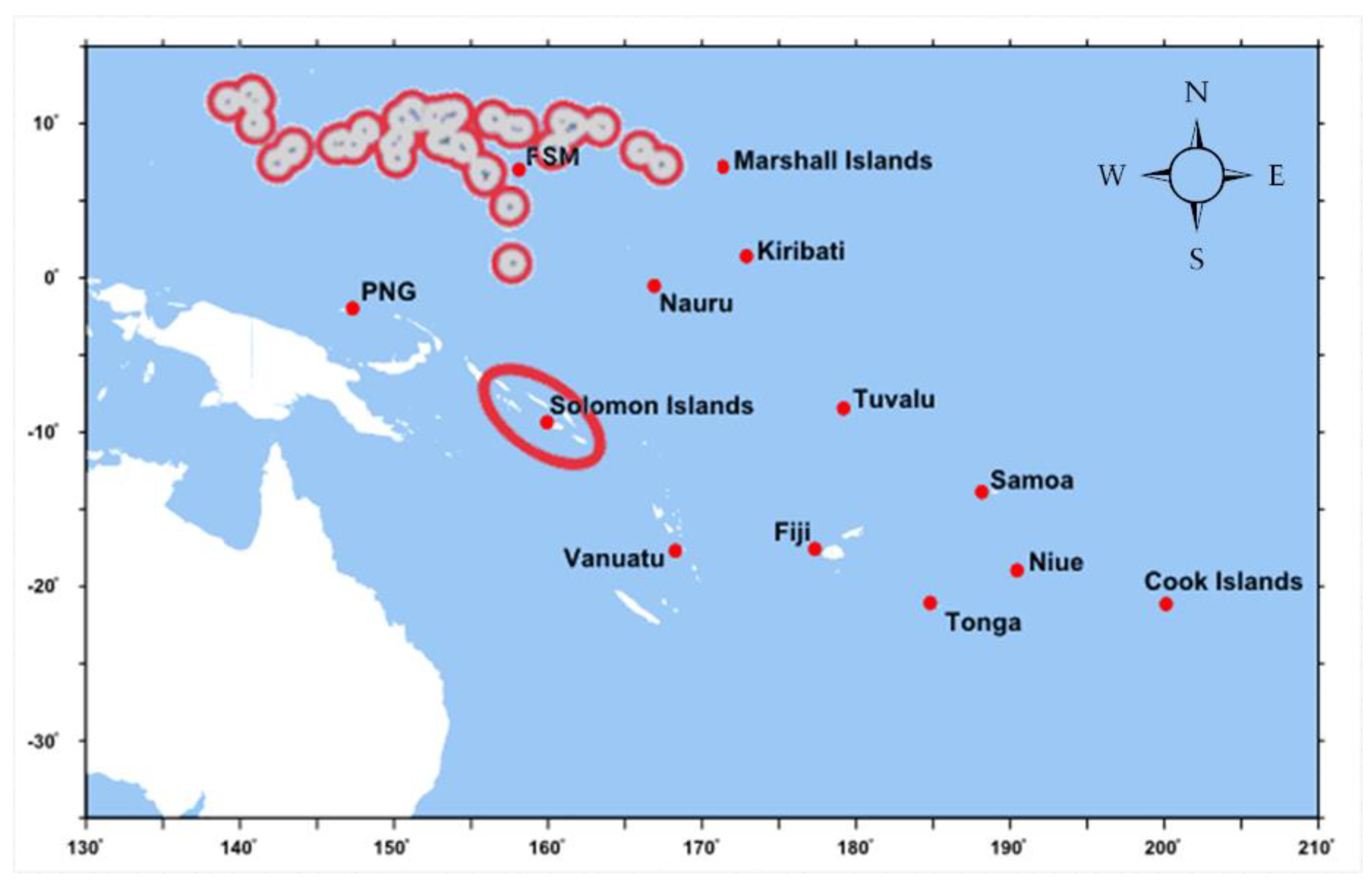
| FSM | Pohnpei | 6°50′59.99″N and 158°12′60.00″E |
| Solomon Islands (SI) | Honiara | 9°25′59.99″S and 159°56′60.00″E |
| Partition | Training | Validation | Testing |
|---|---|---|---|
| SI Oceanic Dataset | September 1994–December 2011 | December 2014–May 2017 | June 2017–February 2023 |
| FSM Oceanic Dataset | December 2001–October 2014 | November 2014–June 2018 | July 2018–February 2023 |
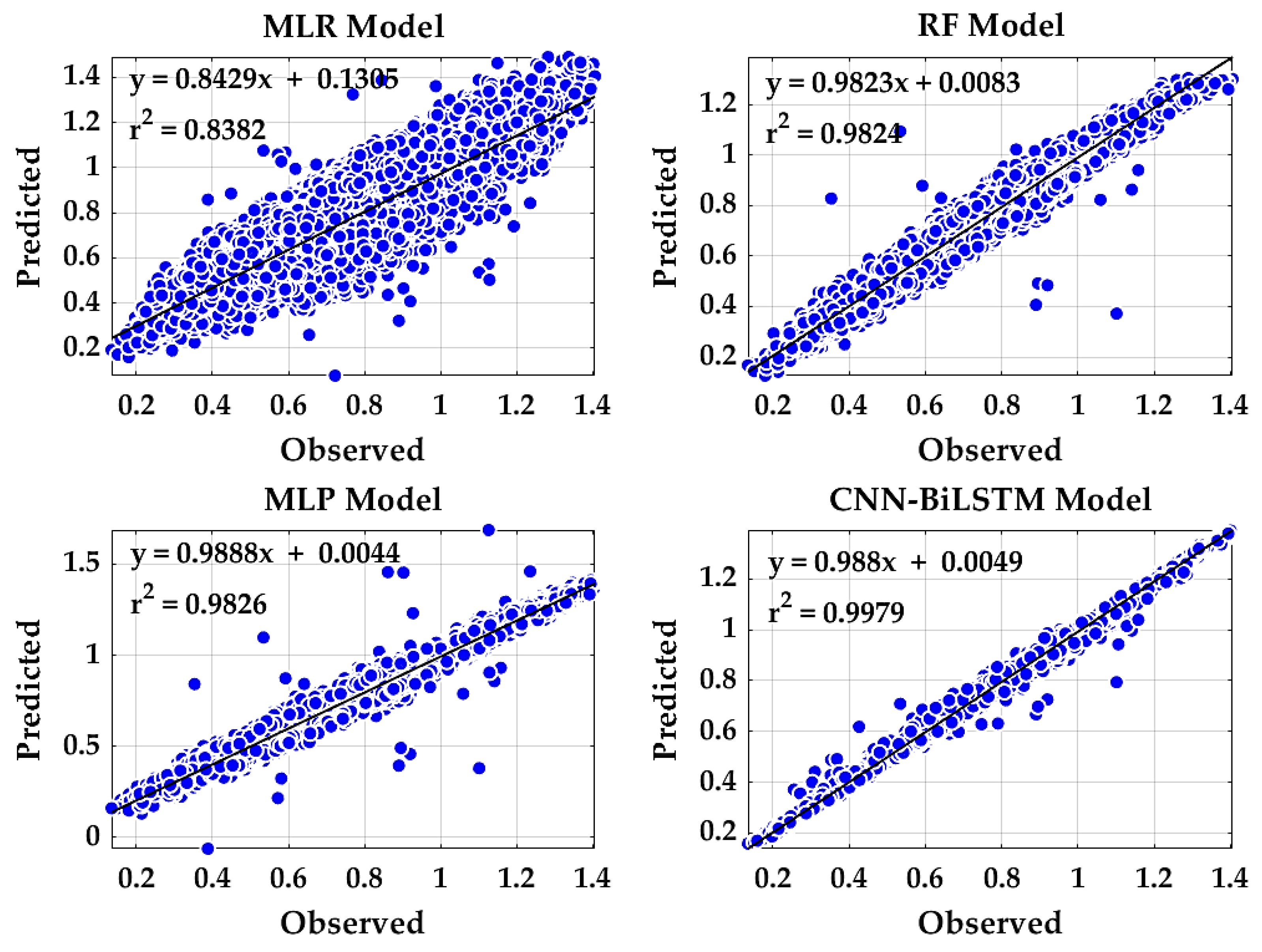
| Model | r | d | LM | RMSE | MAE |
|---|---|---|---|---|---|
| MLR | 0.9155 | 0.9068 | 0.6128 | 0.0886 | 0.0696 |
| RF | 0.9912 | 0.9911 | 0.8775 | 0.0296 | 0.022 |
| MLP | 0.9913 | 0.9911 | 0.8803 | 0.0294 | 0.0215 |
| CNN-BiLSTM | 0.9989 | 0.9987 | 0.9532 | 0.0113 | 0.0084 |
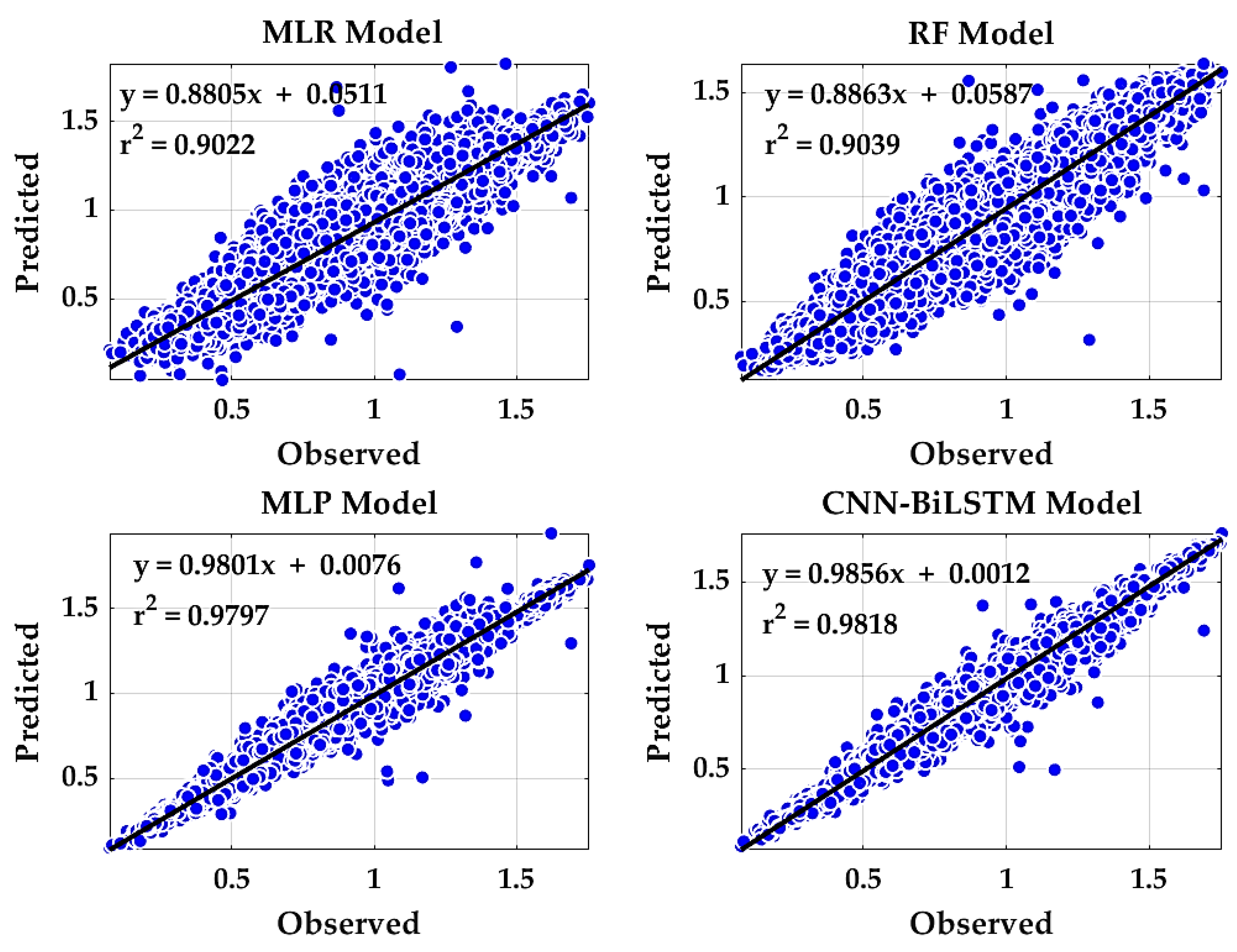
| Model | r | d | LM | RMSE | MAE |
|---|---|---|---|---|---|
| MLR | 0.9499 | 0.9355 | 0.654 | 0.1044 | 0.0821 |
| RF | 0.9507 | 0.9408 | 0.6816 | 0.0982 | 0.0756 |
| MLP | 0.9898 | 0.9885 | 0.8682 | 0.0425 | 0.0313 |
| CNN-BiLSTM | 0.9909 | 0.9891 | 0.8723 | 0.0415 | 0.0303 |
| Study Area | Samples Taken | Training | Testing | Overall Accuracy | Percentage Accuracy | Kappa |
|---|---|---|---|---|---|---|
| Guadalcanal, SI | 330 | 264 | 66 | 0.9834 | 98.34% | 0.92 |
| Pohnpei, FSM | 340 | 272 | 68 | 0.9923 | 99.23% | 0.94 |
| Study Area Wetland Classified Image | 2009 Area | 2022 Area | Detected Decline in Coastal Wetland Area from 2009 to 2022 |
|---|---|---|---|
| Guadalcanal, SI | 12,161.14 ha | 6562.11 ha | 5599.03 ha |
| Pohnpei, FSM | 7371.14 ha | 5960.59 ha | 1410.55 ha |
Disclaimer/Publisher’s Note: The statements, opinions and data contained in all publications are solely those of the individual author(s) and contributor(s) and not of MDPI and/or the editor(s). MDPI and/or the editor(s) disclaim responsibility for any injury to people or property resulting from any ideas, methods, instructions or products referred to in the content. |
© 2024 by the authors. Licensee MDPI, Basel, Switzerland. This article is an open access article distributed under the terms and conditions of the Creative Commons Attribution (CC BY) license (https://creativecommons.org/licenses/by/4.0/).
Share and Cite
Raj, N.; Pasfield-Neofitou, S. Assessment and Prediction of Sea Level and Coastal Wetland Changes in Small Islands Using Remote Sensing and Artificial Intelligence. Remote Sens. 2024, 16, 551. https://doi.org/10.3390/rs16030551
Raj N, Pasfield-Neofitou S. Assessment and Prediction of Sea Level and Coastal Wetland Changes in Small Islands Using Remote Sensing and Artificial Intelligence. Remote Sensing. 2024; 16(3):551. https://doi.org/10.3390/rs16030551
Chicago/Turabian StyleRaj, Nawin, and Sarah Pasfield-Neofitou. 2024. "Assessment and Prediction of Sea Level and Coastal Wetland Changes in Small Islands Using Remote Sensing and Artificial Intelligence" Remote Sensing 16, no. 3: 551. https://doi.org/10.3390/rs16030551
APA StyleRaj, N., & Pasfield-Neofitou, S. (2024). Assessment and Prediction of Sea Level and Coastal Wetland Changes in Small Islands Using Remote Sensing and Artificial Intelligence. Remote Sensing, 16(3), 551. https://doi.org/10.3390/rs16030551