LDnADMM-Net: A Denoising Unfolded Deep Neural Network for Direction-of-Arrival Estimations in A Low Signal-to-Noise Ratio

Abstract

In this paper, we explore the problem of direction-of-arrival (DOA) estimation for a non-uniform linear array (NULA) under strong noise. The compressed sensing (CS)-based methods are widely used in NULA DOA estimations. However, these methods commonly rely on the tuning of parameters, which are hard to fine-tune. Additionally, these methods lack robustness under strong noise. To address these issues, this paper proposes a novel DOA estimation approach using a deep neural network (DNN) for a NULA in a low SNR. The proposed network is designed based on the denoising convolutional neural network (DnCNN) and the alternating direction method of multipliers (ADMM), which is dubbed as LDnADMM-Net. First, we construct an unfolded DNN architecture that mimics the behavior of the iterative processing of an ADMM. In this way, the parameters of an ADMM can be transformed into the network weights, and thus we can adaptively optimize these parameters through network training. Then, we employ the DnCNN to develop a denoising module (DnM) and integrate it into the unfolded DNN. Using this DnM, we can enhance the anti-noise ability of the proposed network and obtain a robust DOA estimation in a low SNR. The simulation and experimental results show that the proposed LDnADMM-Net can obtain high-accuracy and super-resolution DOA estimations for a NULA with strong robustness in a low signal-to-noise ratio (SNR).

1. Introduction

Direction-of-arrive (DOA) estimation is a fundamental problem in array signal processing and is widely applied in radar, sonar, wireless communications, etc. [1,2,3,4,5,6]. DOA estimation can be obtained in a specified array configuration, e.g., linear, rectangular, and circular ones. There are two typical linear array configurations as follows: a uniform linear array (ULA) and a non-uniform linear array (NULA) [7]. Many DOA estimation methods have been investigated over the years focusing on ULA configurations. Compared with ULA configurations, NULA ones can be employed to extend the array aperture and consequently improve the DOA resolution [8,9]. Hence, the DOA estimation in NULA configurations has become a research hotspot.

The DOA estimation problem can be formulated as an optimization of the cost function over the feasible DOA region. In general, the process requires evaluating the cost function for the whole DOA region and searching for that function’s optimum [10,11,12,13]. From this point, subspace methods such as multiple signal classification (MUSIC) can be used for DOA estimation in NULA configurations, which is achieved by approximating the NULA manifold through a Fourier series. These methods rely on the estimation of the received signal covariance matrix and attempt to separate the signal and noise subspaces. However, these methods usually require large snapshots, particularly in a low SNR. Moreover, the search process in this method can increase computational complexity, especially when high spatial resolution is desired.

Another method for DOA estimation in NULA configurations is the use of the compressed sensing (CS) technique [14,15,16]. CS-based methods exploit the sparse characteristics of the target signal in the spatial domain. They treat the DOA estimation as a sparse signal recovery problem and resolve this problem by introducing certain sparse regularizations. Various CS-based methods have been proposed for DOA estimations in NULA configurations, e.g., those of the orthogonal matching pursuit (OMP) [17], iterative shrinkage-thresholding algorithm (ISTA) [18], and alternating direction method of multipliers (ADMM) [19]. However, these methods face two challenges in practical applications. First, the tuning of one or more parameters in these methods is required to guarantee a high performance, which is time-consuming and less robust [20]. Second, the performance of these methods deteriorates significantly under strong noise [21].

Recently, DOA estimations using the deep neural network (DNN) has attracted interest due to fast developments in deep learning (DL) [22,23,24,25,26,27,28,29,30,31,32,33,34,35]. DL-based methods enjoy several advantages over the abovementioned methods. For instance, DL-based methods do not require any specific tuning of the parameters in contrast with CS-based methods. Moreover, they demonstrate resilience to data imperfections, e.g., that of using fewer snapshots. The core of DL-based methods can be summarized as transforming the DOA estimation into a classification task. These methods can obtain high-accuracy DOA estimations by learning features from large-scale datasets. However, the existing DL-based methods usually work in an end-to-end “black-box” manner. This means that their performance mainly depends on the datasets and is potentially unstable. Additionally, the robustness of the network under strong noise is required to be improved.

In this paper, a novel DNN architecture is proposed for DOA estimations in NULA configurations under strong noise. The proposed network mimics the behavior of the denoising-based alternating direction method of multipliers (Dn-ADMM), which is hence dubbed as the learned Dn-ADMM network (LDnADMM-Net). We construct an unfolded DNN structure that maps the iterative processing of the ADMM into a network. In this way, the parameters in the ADMM can be designed as the learnable network weights. Thus, the parameters in the proposed network are fully interpretable and can be adaptively optimized through network training. Furthermore, we develop a denoising module (DnM) with a DnCNN and integrate it into the unfolded DNN. This module can be employed to eliminate the noise, thus providing the anti-noise capability for the proposed network. Extensive simulations and experiments are carried out to demonstrate the performance of the proposed method. The main contributions of this paper are listed as follows:

• We design an unfolded DNN architecture for DOA estimations with NULA configurations in a low SNR. This network is interpretable as its architecture mimics the iterative processing of the ADMM. Moreover, this network can adaptively obtain the optimal parameters in a conventional ADMM through training, thus obtaining stable estimation results.
• We integrate a denoising module into the unfolded DNN. This module can remove the strong noise in observed data, thus enhancing the robustness of the proposed network in a low SNR.

The rest of this paper is organized as follows: In Section 2, we introduce the related works. In Section 3, we describe the signal model in DOA estimations with NULA configurations and the fundamental principles of the ADMM algorithm. In Section 4, we construct the LDnADMM-Net and describe each functional module in detail. In Section 5, we utilize the simulation results to demonstrate the performance of the proposed network. In Section 6, we carry out experiments to verify the feasibility of the proposed method. Finally, the conclusions are given in Section 7.

2. Related Works

We introduce the existing studies in relation to our work in the following two aspects, i.e., model-driven DOA estimation methods and data-driven DOA estimation methods.

2.1. Model-Driven DOA Estimation Methods

In model-driven methods, the DOA estimation problem can be formulated as an optimization model over a feasible DOA region. Then, these methods employ various optimizers to solve this optimization problem, thereby obtaining the DOA values.

Early works for NULA DOA estimations were focused on subspace methods. This method traces back to “Fourier domain root-MUSIC” [10], which was achieved by approximating the NULA array manifold through a Fourier series. There also exist array interpolation techniques that transform the ULA manifold into a NULA manifold [13]. However, this technique is limited by a tradeoff between accuracy and computational complexity.

Recently, DOA estimations using the CS technique have become one hotspot. The CS-based methods treat the DOA estimation as a sparse signal recovery problem and resolve this problem by introducing certain sparse regularizations. In [16], a sparse Bayesian learning (SBL) method was explored to obtain the DOA estimation for arbitrary linear arrays. In [17], a super-resolution DOA estimation method that combines the orthogonal matching pursuit (OMP) algorithm with root-MUSIC was presented for the NULA. In [18], the iterative shrinkage-thresholding algorithm (ISTA) was utilized to obtain high-accuracy and high-resolution DOA estimations for a NULA with 32 elements. In [19], the alternating direction method of multipliers (ADMM) was employed to reach a compromise between complexity, resolution, and accuracy in a DOA estimation.

In summary, the abovementioned methods are based on subspace and sparsity, i.e., they can be categorized as model-driven methods. However, there exist various imperfections of the observed data in practical applications, thus leading to the non-linearity of the signal model. We cannot obtain data that are the same as those in the ideal situation of the assumption. This means that most of these methods under simple assumptions cannot be applied to real applications directly.

2.2. Data-Driven DOA Estimation Methods

Deep learning-based DOA estimations are a kind of data-driven method that does not rely on the ideal assumption of arrays. The DL-based methods can build the propagation model according to the data, which can obtain a high-accuracy DOA estimation by learning features from large-scale datasets [22,23,24,25,26,27].

A deep neural network (DNN) with fully connected (FC) layers was employed in [28] for DOA classification using the signal covariance matrix. Nevertheless, the demonstrated results indicate poor DOA estimation results. A multilayer autoencoder for DOA estimations was proposed in [29] to reduce the influence of noise and array imperfections. However, this network is required to train at each individual SNR. In [30], a deep convolutional neural network (CNN) was presented for DOA estimations in a low SNR. However, this method did not demonstrate significant performance gains in terms of DOA estimations. In [31], the residual neural network (ResNet) was proposed for DOA estimations. Since the ResNet can converge with a very deep structure, it is helpful for achieving higher an estimation accuracy. However, the ResNet estimates DOA values by searching peaks in the recovered spatial spectrum, which limits performance improvement. An artificial neural network was developed in [32] to enlarge the antenna aperture and obtain high-resolution DOA estimations using a self-supervised learning scheme. Similarly, the supervised learning technique in [33] was explored to map a small-size to a larger-size virtual array so as to enlarge the array aperture. However, in both [32,33], the DOA estimator still utilizes the conventional model-driven methods. Thus, the performance gain is limited. In [34], a DNN for beamforming with a single-snapshot sample covariance matrix was proposed in the context of acoustics, which was later extended in [35] to include slightly more snapshots and sources. Such an approach cannot be adopted in a low SNR, where the number of snapshots needs to be considerably higher.

3. Background

3.1. Signal Model

Let us consider a non-uniform linear array with N antennas, as shown in Figure 1. Without loss of generality, the antenna spacings are denoted as d = [d₁, d₂, …, d_N−1] where these antenna spacings are unequal.

Assume that there are M far-field targets impinging on this NULA, the array output vector y is given by

$$\mathbf{y}=\mathbf{A}\mathbf{x}+\mathbf{n}$$

(1)

where

$$\mathbf{y}={\left[\begin{array}{ccccc}{y}_1& \cdots & y_n& \cdots & y_N\end{array}\right]}^{\mathrm{T}} \in {ℂ}^{N\times 1}$$

(2)

$$\mathbf{A}=\left[\begin{array}{ccc}1& \cdots & 1\\ exp\left(-j2\pi d_{1}sin {\theta }_1/\lambda \right)& \cdots & exp\left(-j2\pi d_{1}sin {\theta }_L/\lambda \right)\\ ⋮& \ddots & ⋮\\ exp\left(-j2\pi \left({\displaystyle \sum _{i=1}^{N-1}{d}_i}\right)sin {\theta }_1/\lambda \right)& \cdots & exp\left(-j2\pi \left({\displaystyle \sum _{i=1}^{N-1}{d}_i}\right)sin {\theta }_L/\lambda \right)\end{array}\right] \in {ℂ}^{N\times L}$$

(3)

$$\mathbf{x}={\left[\begin{array}{ccccccccccccc}0& \cdots & x_1& \cdots & 0& \cdots & x_m& \cdots & 0& \cdots & x_M& \cdots & 0\end{array}\right]}^{\mathrm{T}} \in {ℂ}^{L\times 1}$$

(4)

$$\mathbf{n}={\left[\begin{array}{ccccc}{n}_1& \cdots & n_n& \cdots & n_N\end{array}\right]}^{\mathrm{T}} \in {ℂ}^{N\times 1}$$

(5)

where A is the manifold matrix with discretized DOA sampling [θ₁, θ₂, ∙∙∙, θ_L], L is the number of discrete DOA values in the spatial domain, x represents the target complex amplitude, and n denotes the additive white Gaussian noise. It should be noted that x in Equation (4) is a sparse vector with respect to the discretized spatial domain. Namely, the elements in x corresponding to the DOA values where M targets are located are set to the target complex amplitude, and the other L − M sampling points are set to 0.

3.2. ADMM Algorithm for DOA Estimation

According to the ADMM algorithm and the sparsity property, we can formulate the following optimization problem to estimate x in Equation (4):

$$\begin{array}{l}\underset{\mathbf{x}}{min} \frac{1}{2}{‖\mathbf{y}-\mathbf{A}\mathbf{x}‖}_2^2+{\lambda }_{\mathbf{z}}{‖\mathbf{z}‖}_1\\ s.t. \mathbf{x}-\mathbf{z}=0\end{array}$$

(6)

where λ_z controls the sparsity and z denotes an independent auxiliary variable. Given the received echoes y, the purpose of Equation (6) is to seek an optimal sparse vector x that fits Equation (1).

To solve the optimization problem as in Equation (6), we can define the corresponding augmented Lagrangian function as

$$\begin{array}{c}\mathcal{L}(\mathbf{x},\mathbf{z},\mathbf{v},\rho )=\frac{1}{2}{‖\mathbf{y}-\mathbf{A}\mathbf{x}‖}_2^2+{\lambda }_{\mathbf{z}}{‖\mathbf{z}‖}_1+{\mathbf{v}}^{\mathrm{T}}(\mathbf{x}-\mathbf{z})+\frac{\rho }{2}{‖\mathbf{x}-\mathbf{z}‖}_2^2\\ \stackrel{\mathbf{u}={\mathbf{v}}^{\mathrm{T}}/\rho }{\iff }\mathcal{L}(\mathbf{x},\mathbf{z},\mathbf{u})=\frac{1}{2}{‖\mathbf{y}-\mathbf{A}\mathbf{x}‖}_2^2+{\lambda }_{\mathbf{z}}{‖\mathbf{z}‖}_1+\frac{\rho }{2}{‖\mathbf{x}-\mathbf{z}+\mathbf{u}‖}_2^2\end{array}$$

(7)

where ρ > 0 is the penalty parameter, v^T is the Lagrangian multiplier representing the dual variable, and u = v^T / ρ denotes the scaled dual variable.

Using the ADMM algorithm, x, z, and u can be updated in an alternating or sequential manner. Referring to [36,37], these variables of the k-th iteration can be optimized by resolving the following subproblems:

$${\mathbf{x}}_k=\underset{\mathbf{x}}{argmin}\left\{\frac{1}{2}{‖{\mathbf{y}}_{k-1}-\mathbf{A}{\mathbf{x}}_{k-1}‖}_2^2+{\lambda }_{\mathbf{z}}{‖{\mathbf{z}}_{k-1}‖}_1+\frac{\rho }{2}{‖{\mathbf{x}}_{k-1}-{\mathbf{z}}_{k-1}+{\mathbf{u}}_{k-1}‖}_2^2\right\}$$

(8)

$${\mathbf{z}}_k=\underset{\mathbf{z}}{argmin}\left\{\frac{1}{2}{‖{\mathbf{y}}_{k-1}-\mathbf{A}{\mathbf{x}}_k‖}_2^2+{\lambda }_{\mathbf{z}}{‖{\mathbf{z}}_{k-1}‖}_1+\frac{\rho }{2}{‖{\mathbf{x}}_k-{\mathbf{z}}_{k-1}+{\mathbf{u}}_{k-1}‖}_2^2\right\}$$

(9)

$${\mathbf{u}}_k=\underset{\mathbf{u}}{argmin}\left\{\frac{1}{2}{‖{\mathbf{y}}_{k-1}-\mathbf{A}{\mathbf{x}}_k‖}_2^2+{\lambda }_{\mathbf{z}}{‖{\mathbf{z}}_k‖}_1+\frac{\rho }{2}{‖{\mathbf{x}}_k-{\mathbf{z}}_k+{\mathbf{u}}_{k-1}‖}_2^2\right\}$$

(10)

By updating these three variables in an alternating or sequential fashion, we can obtain the optimal sparse vector x that fits Equation (1), thus achieving the final DOA estimation results.

4. Proposed Method

The major issue of the above ADMM algorithm is how to choose the hyperparameters, which pose a high impact on the convergence speed and estimation accuracy. Additionally, the high noise in Equation (1) will lead to a significant decline in estimation accuracy. To address these issues, we aim to map the ADMM solver into a deep unfolded neural network and integrate a denoising module into this network. The network architecture is described as follows.

4.1. Network Structure

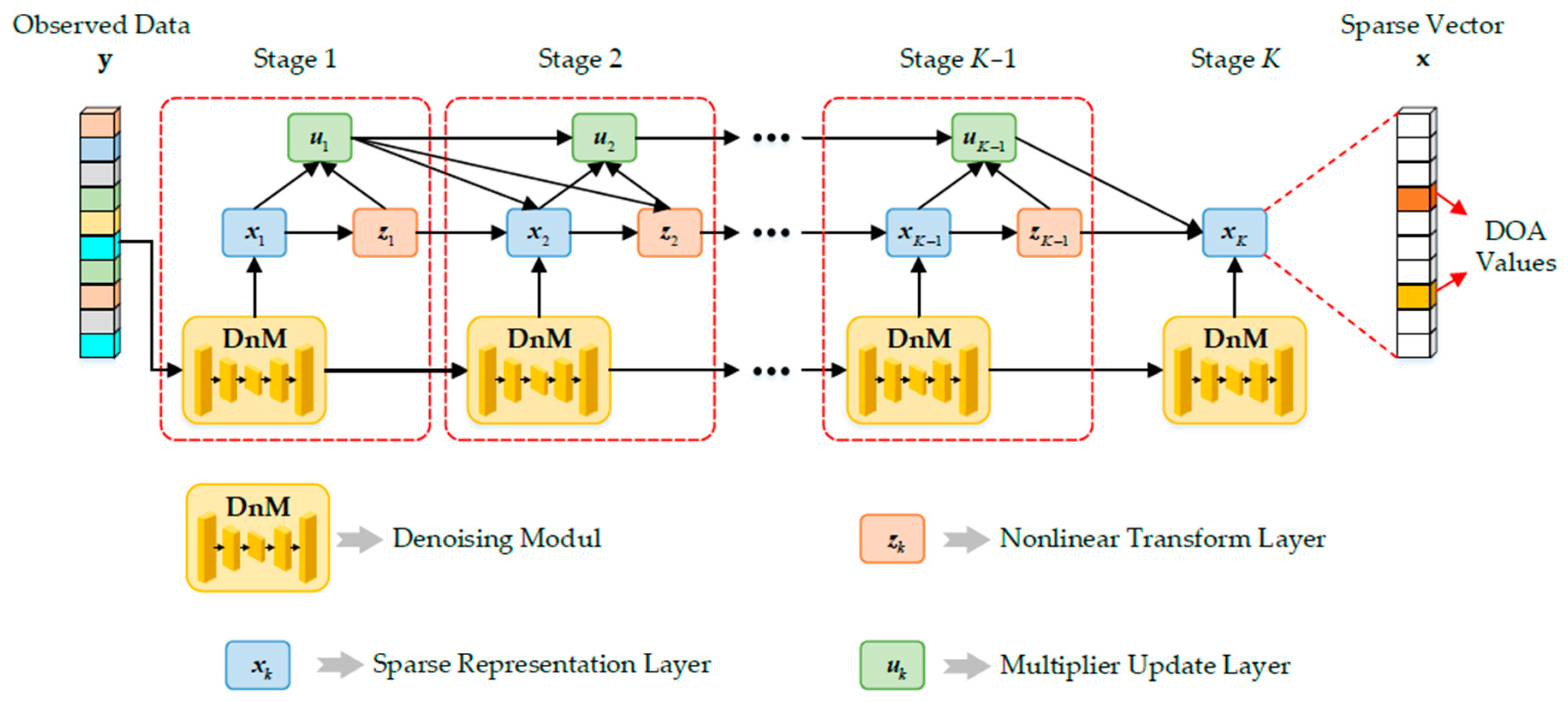
Figure 2 shows the LDnADMM-Net structure. The basic idea of the proposed network is to unfold the previous iterative ADMM solver as an unfolded deep neural network that consists of a fixed number of layers. On this basis, the input of each iteration is subjected to a denoising module (DnM). The LDnADMM-Net is composed of K stages in which the k-th stage corresponds to the k-th iteration of the ADMM algorithm with a denoising input. The network input is the observed data y. The network output is the optimal sparse vector x, and we can obtain the DOA values from that.

As shown in Figure 2, each stage of the LDnADMM-Net consists of a denoising module and three learnable layers. We define these learnable layers as the sparse representation layer, non-linear transform layer, and multiplier update layer. Moreover, these learnable layers correspond to the analytical solutions of the subproblems in the ADMM algorithm, respectively. Next, we introduce the denoising module and three learnable layers in detail.

4.2. Module Design

4.2.1. Denoising Module

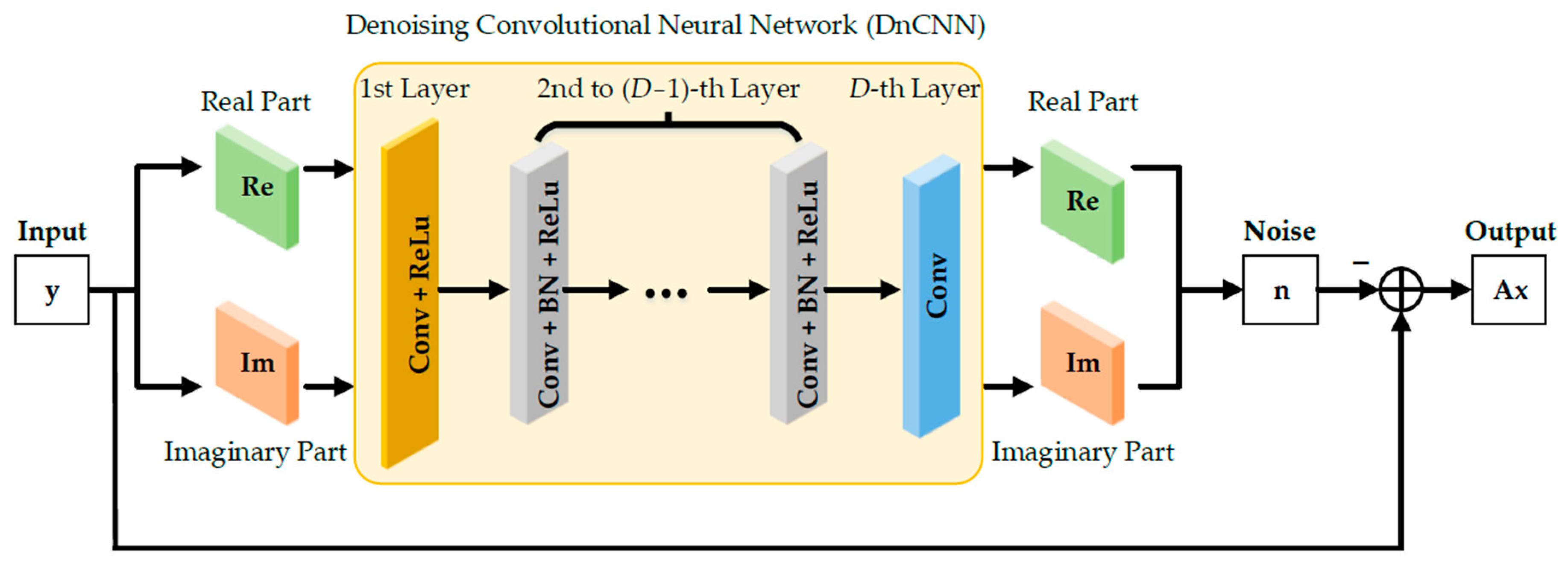
The denoising convolutional neural network (DnCNN) can be used to remove the additive Gaussian white noise, which has been widely applied in image denoising [38,39]. However, in the field of image denoising, the data in the conventional DnCNN are usually real-valued. Thus, this network cannot be directly applied to array signal processing in which the observed data are complex-valued. For this reason, we modify the DnCNN to design the de-noising module, as illustrated in Figure 3. This modified DnCNN is partitioned into real and imaginary channels to perform complex multiplication for complex-valued operations.

The output of the modified DnCNN is the noise. Then, we can remove it from the original observed data, thus obtaining the clean signal as the output of the DnM. The structure of the DnM can be summarized as follows:

• Decompose the real and imaginary parts of the input data to obtain a dual-channel input. Herein, assume that the number of antennas is N and the dimension of the decomposed input is 1 × N × 2.
• The first layer of the modified DnCNN consists of convolution (Conv) and the rectified linear unit (ReLu). This layer performs convolution operations with p convolution kernels (1 × q × 2), thus obtaining the feature maps (1 × N × p). Then, these feature maps are activated with the ReLu function.
• The second to (D − 1)-th layers of the modified DnCNN are composed of convolution (Conv), batch normalization (BN), and the rectified linear unit (ReLu). These layers perform convolution operations with p convolution kernels (1 × q × p) to output the feature maps (1 × N × p). These feature maps are further standardized in batches and non-linearly activated through the ReLu function to obtain the final feature maps.
• The D-th layer of the modified DnCNN is only composed of convolution (Conv). This layer performs convolution operations with two convolution kernels (1 × q × p), thus obtaining the real and imaginary parts of the estimated noise (1 × N × 2).
• Finally, the real and imaginary parts of the estimated noise are reconstructed into complex-valued noise. We can remove it from the original input data to obtain the clean signal as the DnM output.

In the modified DnCNN, there are two crucial parameters, i.e., the number of convolutional kernels p and the network depth D. The convolution layer is mainly used for automatic feature extraction, and increasing the number of convolution kernels can extract more features. On the other hand, it is customary to use a stack of multiple small convolution kernels instead of a larger one, which can provide powerful non-linear fitting capabilities for the network. However, excessive convolutional kernels may lead to overfitting in network training. Additionally, the network depth is related to the size of the convolutional kernels. Referring to [40], the ideal depth is advised to be set to (N − 1)/(q − 1) or more where q represents the length of the convolutional kernel.

4.2.2. Sparse Representation Layer

The sparse representation layer corresponds to the iteration of sparse vector x as in Equation (8). According to the derivation rule, Equation (8) can be simplified as follows:

$$\left[\frac{1}{2}{\nabla }_{\mathbf{x}}{\left({\mathbf{y}}_{k-1}-\mathbf{A}{\mathbf{x}}_{k-1}\right)}^{\mathrm{H}}\left({\mathbf{y}}_{k-1}-\mathbf{A}{\mathbf{x}}_{k-1}\right)+\frac{\rho }{2}{\nabla }_{\mathbf{x}}{\left({\mathbf{x}}_{k-1}-{\mathbf{z}}_{k-1}+{\mathbf{u}}_{k-1}\right)}^{\mathrm{H}}\left({\mathbf{x}}_{k-1}-{\mathbf{z}}_{k-1}+{\mathbf{u}}_{k-1}\right)\right]=0$$

(11)

The solutions to the above subproblem can be derived as follows:

$${\mathbf{x}}_k={\left({\mathbf{A}}^{\mathrm{H}}\mathbf{A}+\rho \mathbf{I}\right)}^{-1}\left({\mathbf{A}}^{\mathrm{H}}{\mathbf{y}}_{k-1}+\rho \left({\mathbf{z}}_{k-1}-{\mathbf{u}}_{k-1}\right)\right)$$

(12)

where I denotes the identity matrix.

This solution can be further rewritten as follows:

$${\mathbf{x}}_k={\left({\mathbf{W}}_1\right)}_k{\mathbf{y}}_{k-1}+{\left({\mathbf{W}}_2\right)}_k\left({\mathbf{z}}_{k-1}-{\mathbf{u}}_{k-1}\right)$$

(13)

where W₁ and W₂ represent the learnable weights in the sparse representation layer, and they can be defined as follows:

$${\left({\mathbf{W}}_1\right)}_k={\left({\mathbf{A}}^{\mathrm{H}}\mathbf{A}+\rho \mathbf{I}\right)}^{-1}{A}^H$$

(14)

$${\left({\mathbf{W}}_2\right)}_k=\rho {\left({\mathbf{A}}^{\mathrm{H}}\mathbf{A}+\rho \mathbf{I}\right)}^{-1}$$

(15)

Additionally, since the input data are complex-valued, the sparse representation layer involves complex-valued multiplication operations. Herein, we provide the complex-valued multiplication operational form for Equation (13), which can be expressed as follows:

$$\left\{\begin{array}{ll}{\left({\mathbf{x}}_k\right)}_R& ={\left({\left({\mathbf{W}}_1\right)}_k\right)}_R{\left({\mathbf{y}}_{k-1}\right)}_R-{\left({\left({\mathbf{W}}_1\right)}_k\right)}_I{\left({\mathbf{y}}_{k-1}\right)}_I\\ & +{\left({\left({\mathbf{W}}_2\right)}_k\right)}_R\left({\left({\mathbf{z}}_{k-1}\right)}_R-{\left({\mathbf{u}}_{k-1}\right)}_R\right)-{\left({\left({\mathbf{W}}_2\right)}_k\right)}_I\left({\left({\mathbf{z}}_{k-1}\right)}_I-{\left({\mathbf{u}}_{k-1}\right)}_I\right)\\ {\left({\mathbf{x}}_k\right)}_I& ={\left({\left({\mathbf{W}}_1\right)}_k\right)}_R{\left({\mathbf{y}}_{k-1}\right)}_I+{\left({\left({\mathbf{W}}_1\right)}_k\right)}_I{\left({\mathbf{y}}_{k-1}\right)}_R\\ & +{\left({\left({\mathbf{W}}_2\right)}_k\right)}_R\left({\left({\mathbf{z}}_{k-1}\right)}_I-{\left({\mathbf{u}}_{k-1}\right)}_I\right)+{\left({\left({\mathbf{W}}_2\right)}_k\right)}_I\left({\left({\mathbf{z}}_{k-1}\right)}_R-{\left({\mathbf{u}}_{k-1}\right)}_R\right)\end{array}\right.$$

(16)

where (∙)_R and (∙)_I represent the real and imaginary parts, respectively.

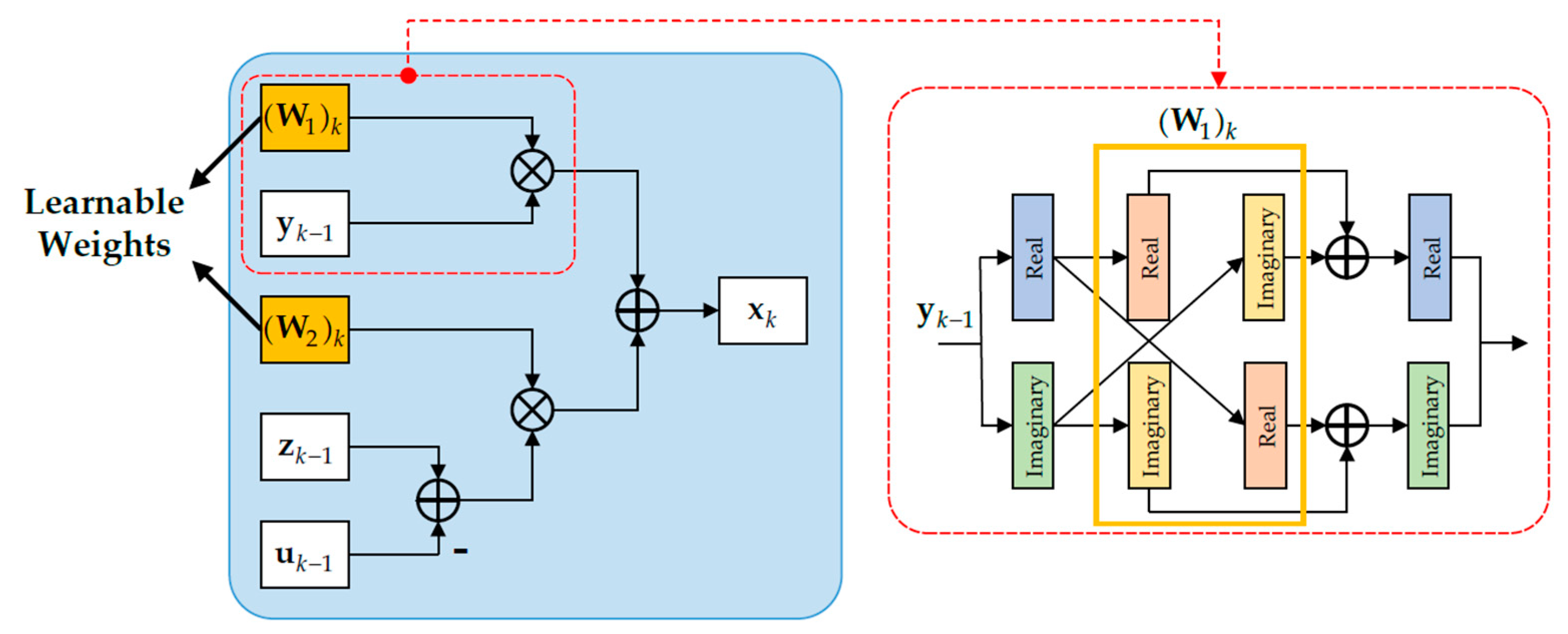
Based on the above derivation, we can construct the structure of the sparse representation layer in the LDnADMM-Net, as shown in Figure 4. Moreover, two parallel propagation lines are used in this layer to calculate the real and imaginary parts, respectively. Information is exchanged between the two propagation lines to ensure that the network can provide complex-valued multiplication operations (see the right picture of Figure 4). It should be noted that this manner is also applicable to the complex-valued multiplication operations involved in the other layers.

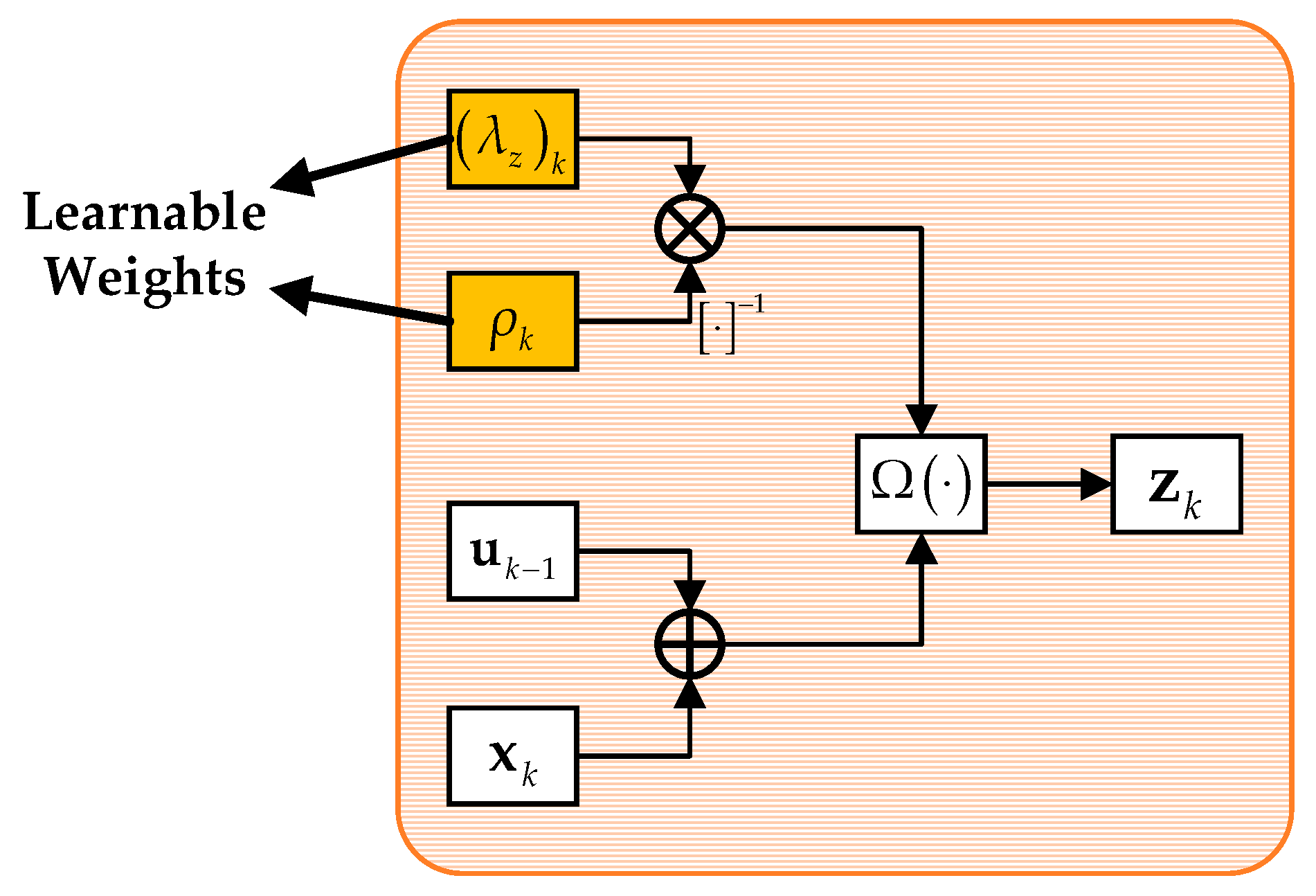
4.2.3. Non-linear Transform Layer

Similarly, the non-linear transform layer corresponds to the iteration of the independent auxiliary variable z as in Equation (9). Using the derivation rule, Equation (9) can be simplified as follows:

$${\lambda }_{\mathbf{z}}{\nabla }_{\mathbf{z}}{‖{\mathbf{z}}_{k-1}‖}_1+\frac{\rho }{2}{\nabla }_{\mathbf{z}}{\left({\mathbf{x}}_k-{\mathbf{z}}_{k-1}+{\mathbf{u}}_{k-1}\right)}^{\mathrm{H}}\left({\mathbf{x}}_k-{\mathbf{z}}_{k-1}+{\mathbf{u}}_{k-1}\right)=0$$

(17)

This question can be simplified as follows:

$$\frac{{\lambda }_{\mathbf{z}}}{\rho }{\nabla }_{\mathbf{z}}{‖{\mathbf{z}}_{k-1}‖}_1+{\mathbf{z}}_{k-1}={\mathbf{x}}_k+{\mathbf{u}}_{k-1}$$

(18)

The solution of Equation (23) can be derived as follows:

$${\mathbf{z}}_k={\mathsf{\Omega }}_{{\left({\lambda }_{\mathbf{z}}\right)}_k/{\rho }_k}\left({\mathbf{x}}_k+{\mathbf{u}}_{k-1}\right)$$

(19)

where ${\mathsf{\Omega }}_{{\lambda }_{\mathbf{z}}/\rho }\left(\cdot \right)$ is a soft thresholding function corresponding to the sparse regularization and can be expressed as follows:

$${\mathsf{\Omega }}_{{\lambda }_{\mathbf{z}}/\rho }\left(a\right)=\left\{\begin{array}{ll}a-{\lambda }_{\mathbf{z}}/\rho ,& a>{\lambda }_{\mathbf{z}}/\rho \\ 0,& \left|a\right|\le {\lambda }_{\mathbf{z}}/\rho \\ a+{\lambda }_{\mathbf{z}}/\rho ,& a<-{\lambda }_{\mathbf{z}}/\rho \end{array}\right.$$

(20)

This layer also involves complex-valued operations, which can be expressed as follows:

$${\mathbf{z}}_k={\mathsf{\Omega }}_{{\left({\lambda }_{\mathbf{z}}\right)}_k/{\rho }_k}\left({\left({\mathbf{x}}_k+{\mathbf{u}}_{k-1}\right)}_R\right)+j\times {\mathsf{\Omega }}_{{\left({\lambda }_{\mathbf{z}}\right)}_k/{\rho }_k}\left({\left({\mathbf{x}}_k+{\mathbf{u}}_{k-1}\right)}_I\right)$$

(21)

To sum up, the structure of the non-linear transform layer is developed in Figure 5.

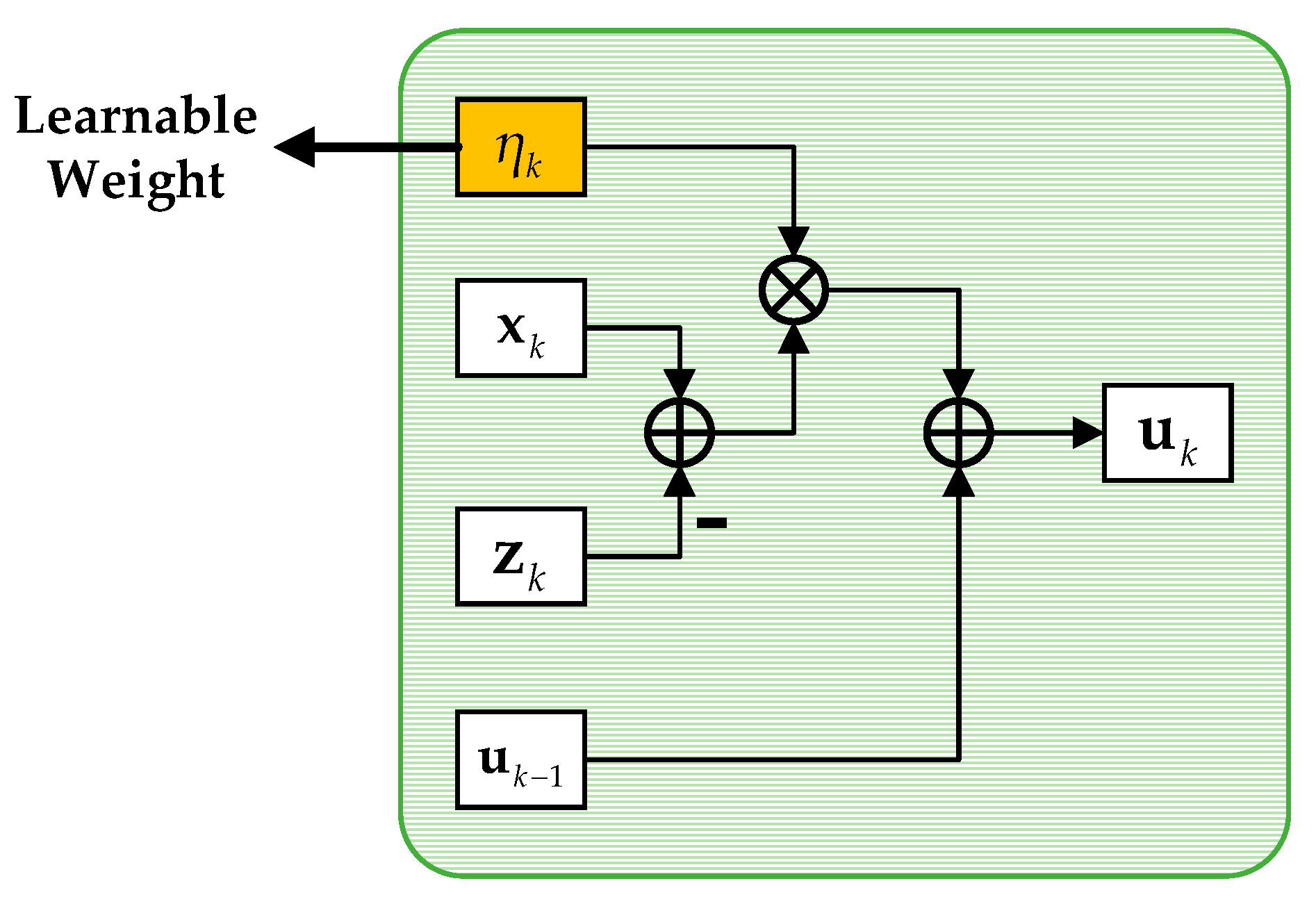
4.2.4. Multiplier Update Layer

By expanding Equation (10), we can obtain the simplified subproblem of the scaled dual variable u as follows:

$$\frac{\rho }{2}{\nabla }_u{\left({\mathbf{x}}_k-{\mathbf{z}}_k+{\mathbf{u}}_{k-1}\right)}^{\mathrm{H}}\left({\mathbf{x}}_k-{\mathbf{z}}_k+{\mathbf{u}}_{k-1}\right)=0$$

(22)

The solution of the above subproblem can be derived as follows:

$${\mathbf{u}}_k={\mathbf{u}}_{k-1}+{\eta }_k\left({\mathbf{x}}_k-{\mathbf{z}}_k\right)$$

(23)

where ${\eta }_k$ represents an update rate for the Lagrangian multiplier, which can be defined as the learnable weight in the multiplier update layer.

Obviously, the multiplier update layer only involves complex-valued sum operations, so it can be directly implemented in the proposed network. The structure of the multiplier update layer is displayed in Figure 6.

4.3. Loss Function

For the whole LDnADMM-Net, the mean square error (MSE) is adopted to ensure the correctness of the output. The label of the i-th input data is a discrete vector corresponding to different DOA values. In this label, the antennas where the targets are located can be defined as the amplitude and phase of the target, and the rest are set to 0. Since the network output and the label are complex-valued vectors, this loss function is formulated as follows:

$$Los{s}_{Net}=\frac{1}{Num}\left({\displaystyle \sum _{i=1}^{Num}{‖{\left(\mathcal{F}\left({\mathbf{y}}^{\left(i\right)}\right)\right)}_R-{\mathbf{L}}_R^{\left(i\right)}‖}_2^2}+{\displaystyle \sum _{i=1}^{Num}{‖{\left(\mathcal{F}\left({\mathbf{y}}^{\left(i\right)}\right)\right)}_I-{\mathbf{L}}_I^{\left(i\right)}‖}_2^2}\right)$$

(24)

where Num is the total number of the training data and $\mathcal{F}\left({\mathbf{y}}^{\left(\mathbf{i}\right)}\right)$ and L denote the output and the label of the i-th input data.

Moreover, for the denoising module, we choose the MSE to measure the similarity between the estimated noise and the real noise, which can be represented as follows:

$$Los{s}_{DnM}=\frac{1}{Num\times N}\left({\displaystyle \sum _{i=1}^{Num}{\Vert {\left(\mathcal{R}\left({\mathbf{y}}^{\left(i\right)}\right)\right)}_R-{\left({\mathbf{y}}^{\left(i\right)}-{\mathbf{x}}^{\left(i\right)}\right)}_R\Vert }_2^2}+{\displaystyle \sum _{i=1}^{Num}{‖{\left(\mathcal{R}\left({\mathbf{y}}^{\left(i\right)}\right)\right)}_I-{\left({\mathbf{y}}^{\left(i\right)}-{\mathbf{x}}^{\left(i\right)}\right)}_I‖}_2^2}\right)$$

(25)

where $\mathcal{R}\left({\mathbf{y}}^{\left(\mathrm{i}\right)}\right)$ represents the estimated noise, i.e., the output of the proposed DnCNN, and N is the number of the array antenna.

In conclusion, the total loss function of the proposed method can be summarized as follows:

$$Loss=Los{s}_{Net}+\delta \cdot Los{s}_{DnM}$$

(26)

where δ is used to adjust the weight of these two loss functions.

4.4. Complexity Analysis

Although the training process is off-line and it is unnecessary to consider the time cost, it is still required to assess the computational efficiency for the trained LDnADMM-Net. Therefore, we analyze the computational complexity of the proposed network, including the DnM and the three learnable layers.

The operations involved in the implementation of the DnM are mainly convolution operations. The DnCNN used in the DnM consists of D layers with convolution operations. We assume that the size of the convolution kernel is q, the length of feature map is N, and the number of input channels and output channels is equal to the number of convolution kernels p. Referring to [41], the computational complexity per layer in the DnCNN is O(qNp²). Therefore, the computational complexity of the D layers in the DnCNN can be calculated as O(DqNp²).

The operations involved in the implementation of the three learnable layers are mainly the inverse operations of the matrix, i.e., the updating for x. In Equation (14) and Equation (15), the length of the vector A is L where L denotes the number of discrete DOA values in the spatial domain. Thus, we can obtain the computational complexity of the three learnable layers in each stage, which is approximated as O(L³).

To sum up, the computational complexity per stage in the LDnADMM-Net is O(L³ + DqNp²). In total, the computational complexity of the proposed network can be approximated as O(K(L³ + DqNp²)) where K is the number of stages.

Table 1. Computational complexity of different methods.

Method	Computational Complexity
OMP	O(ML3) 1
ADMM	O(KL3)
ADMM-Net	O(KL3)
LDnADMM-Net	O(K(L3 + DqNp2))

¹ M denotes the number of targets.

compares the computational complexity of the proposed network with three related methods, including those of the OMP, ADMM, and ADMM-Net. We can see that the LDnADMM-Net has the heaviest computational complexity, while the other methods have approximately equal complexity. The increase in complexity of the LDnADMM-Net is mainly caused by the integration of the DnCNN.

5. Simulations

This section describes the numerical simulations conducted to evaluate the performance of the LDnADMM-Net and demonstrate its effectiveness and advantages. Two typical scenarios are considered in the simulations. One scenario contains a one point target, while the other scenario consists of two point targets. In the first scenario, we focus on the improvement of the denoising module and the estimation accuracy of the proposed network. In the scenario of the two point targets, we focus on the super-resolution performance and the estimation accuracy of the proposed network.

5.1. Parameters Setting and Evaluation Metrics

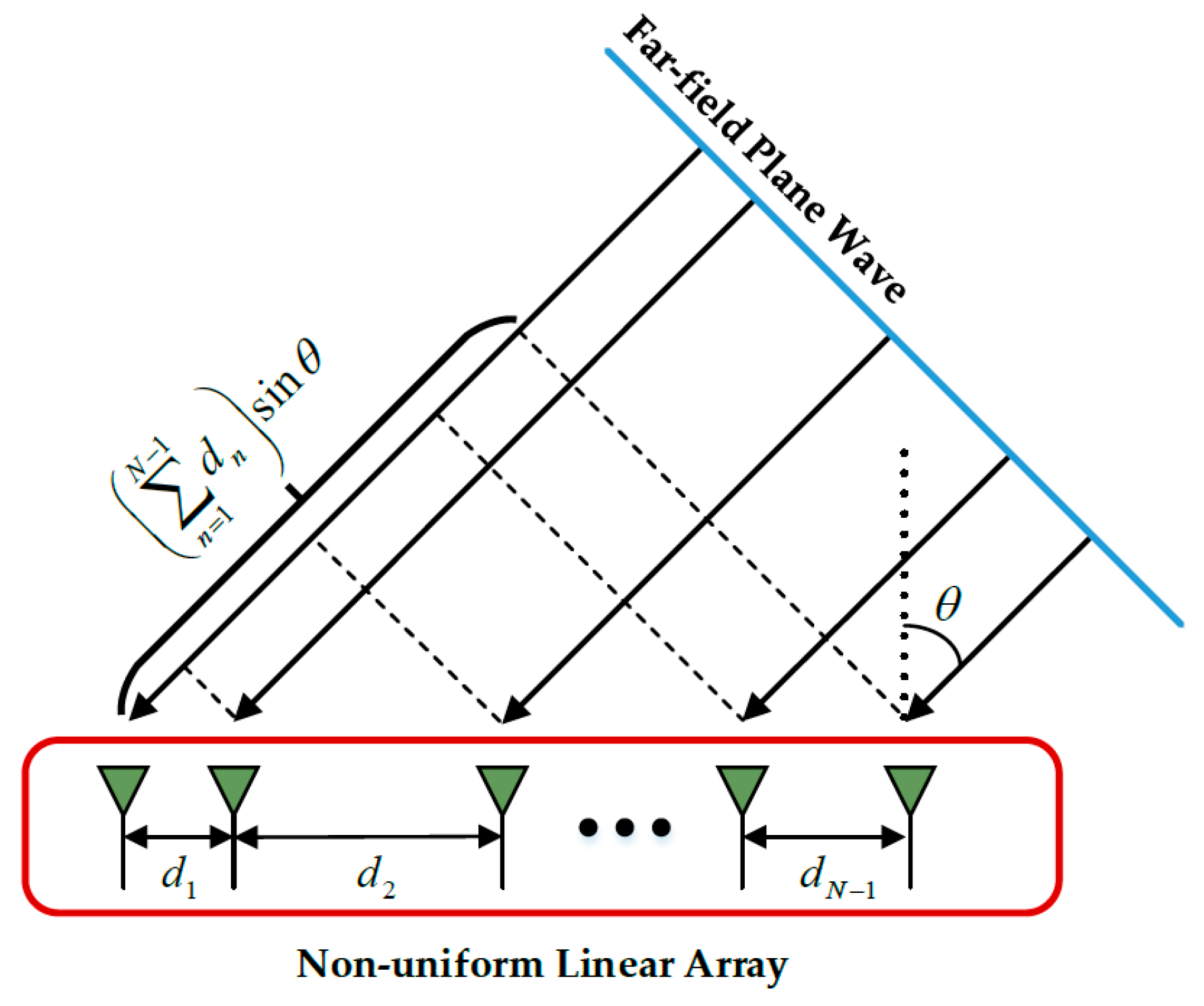
In this subsection, we first introduce the non-uniform linear array configuration used in this work. Then, the parameter setting and the training dataset are given. Finally, we define the metrics used to evaluate the proposed network.

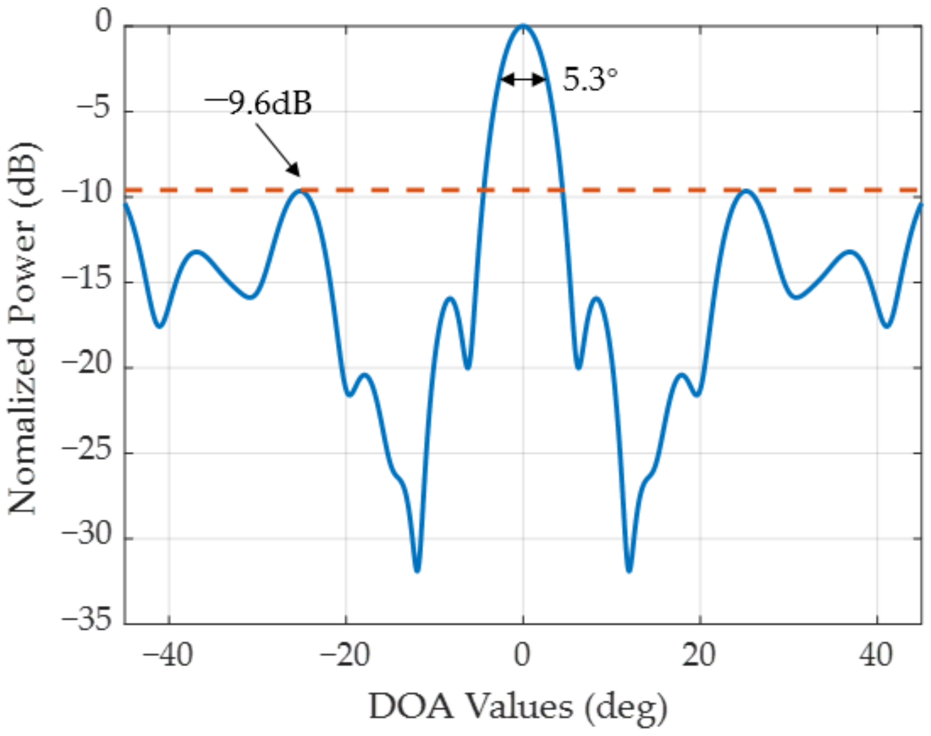
5.1.1. NULA Configuration and Antenna Pattern

The NULA is composed of 12 antennas, which can be set to [0, 3, 5, 6, 9, 10, 11, 13, 14, 15, 17, 19] d (d = λ/2) [42]. Figure 7 displays the antenna pattern of this NULA with the beam pointing at 0°. It can be observed that the beamwidth and the peak sidelobe ratio of this array are 5.3° and −9.6 dB, respectively.

5.1.2. Network Parameters and Training Datasets

The parameters of the LDnADMM-Net are given in

Table 2. The parameters of the LDnADMM-Net.

	Parameters	Value
ADMM	Initial sparsity constraint λz	0.05
	Initial penalty parameter ρ	5
	Initial update rate η	1
	Stage K	10
DnM	Number of convolutional kernels p	64
	Length of convolutional kernel q	3
	Network depth D	15
	Batch size	256
	Learning rate	10−4

. Additionally, we use the Adam optimizer for the DnM training, which can be found in the references of [43,44].

As mentioned in Section 4.2.1, the number of convolutional kernels p and the network depth D will pose a high impact on the DnM. Therefore, we analyze the convergence of DnM training under different parameter settings, as given in

Table 3. The convergence of DnM training versus the number of convolutional kernels p (D = 15).

Values of p	16	32	64	128
Loss after Convergence	0.0884	0.0838	0.0810	0.0808
Training Time (min)	18.54	19.31	20.16	21.32

and

Table 4. The convergence of DnM training versus the network depth D (p = 64).

Values of D	11	13	15	17	19
Loss after convergence	0.0818	0.0816	0.0810	0.0810	0.0812
Training time (min)	15.13	18.21	20.16	21.77	22.97

. It can be found that the DnM can obtain optimal results with p = 64 and D = 15.

The DL-based DOA estimation method under a large field of view (FOV) requires “Big Data” for training. This is caused through the increase in discretized DOA sampling points. To reduce the dependence of the LDnADMM-Net on data, we preprocess the observed data using spatial filters [45] to simplify the FOV by approximately ±θ_3dB (set to ±6° in this work) where θ_3dB represents the beamwidth.

The training dataset can be divided into two groups, which are generated by one random target and two random targets. Based on the above preprocessing, the first dataset is composed of 50,000 samples in which the DOA value of one target is randomly selected from −6° to 6° with an interval of 0.1°. Its SNR is within [−5 dB, 5 dB] with an interval of 1 dB.

Correspondingly, the second dataset also consists of 50,000 samples. Each sample is generated by two random targets. The distribution of their DOA values and SNRs is consistent with the first dataset, but ensuring that the DOA values of these two targets are not equal during sample generation is required.

5.1.3. Evaluation Metrics

We employ five evaluation metrics to comprehensively evaluate the effectiveness of the proposed method.

First, the mean square error (MSE) is used to evaluate the performance of the LDnADMM-Net in terms of denoising. The MSE represents the deviation between the estimated noise (using DnM) and the real noise and can be defined as follows:

$$\mathrm{MSE}=\frac{{\displaystyle \sum _{i=1}^{N_{len}}{\left({\mathcal{R}}_i-n_i\right)}^2}}{N_{len}}$$

(27)

where N_len represents the noise length, ${\mathcal{R}}_i$ is the estimated noise, and n_i represents the real noise.

Second, in the scenario of one target, we further adopt the output SNR (SNR_out) to visualize the denoising effect, which is defined as follows:

$${\mathrm{SNR}}_{out}=10lo{g}_{10}\frac{S_0^2}{N_0^2}$$

(28)

where $S_0^2$ is the average energy inside the resolution unit, $N_0^2$ is the average energy outside the resolution unit, and the length of the resolution unit is the beamwidth.

Third, the strong noise may lead to incorrect DOA estimation results. To this end, we defined the success rate (SR) of the DOA estimation in the scenario of one target, which is expressed as follows:

$$\mathrm{SR}=p\left(\left|\stackrel{⌢}{\theta }-\theta \right|<\frac{{\theta }_{3\mathrm{dB}}}{2}\right)$$

(29)

where θ_3dB is the beamwidth and θ and $\stackrel{⌢}{\theta }$ denote the real and estimated DOA value, respectively.

Fourth, the probability of resolution (PoR) is used to assess the super-resolution performance in the scenario of two targets. The PoR [45,46] is a typical performance indicator used for evaluating high-resolution algorithms and can be defined as follows:

$$\mathrm{PoR}=p\left(\max \left\{\left|{\stackrel{⌢}{\theta }}_1-{\theta }_1\right|,\left|{\stackrel{⌢}{\theta }}_2-{\theta }_2\right|\right\}<\frac{\left|{\theta }_1-{\theta }_2\right|}{2}\right)$$

(30)

where θ₁ and θ₂ denote the real values of two targets and ${\stackrel{⌢}{\theta }}_1$ and ${\stackrel{⌢}{\theta }}_2$ represent the estimated values.

Fifth, we adopt the root mean square error (RMSE) to evaluate the DOA accuracy, which is defined as follows:

$$\mathrm{RMSE}=\sqrt{\frac{1}{S}{\displaystyle \sum _{s=1}^S{\left({\stackrel{⌢}{\theta }}_i-{\theta }_i\right)}^2}}$$

(31)

where S denotes the number of samples. It is noted that we only counted the RMSE under a successful DOA estimation.

5.2. Simulation Results of One Target

In this subsection, we construct a testing dataset with one target. The DOA value of the target is randomly sampled within [−6°, 6°]. Its SNR is selected from −10 dB to 5 dB with an interval of 1 dB. Specifically, 1000 samples with random DOA values are generated for each SNR, while the DOA values are fixed with different SNRs. We added an SNR region of [−10 dB, −5 dB] compared with the training dataset, which can facilitate the generalization analysis in a low SNR.

5.2.1. Performance for Signal Denoising

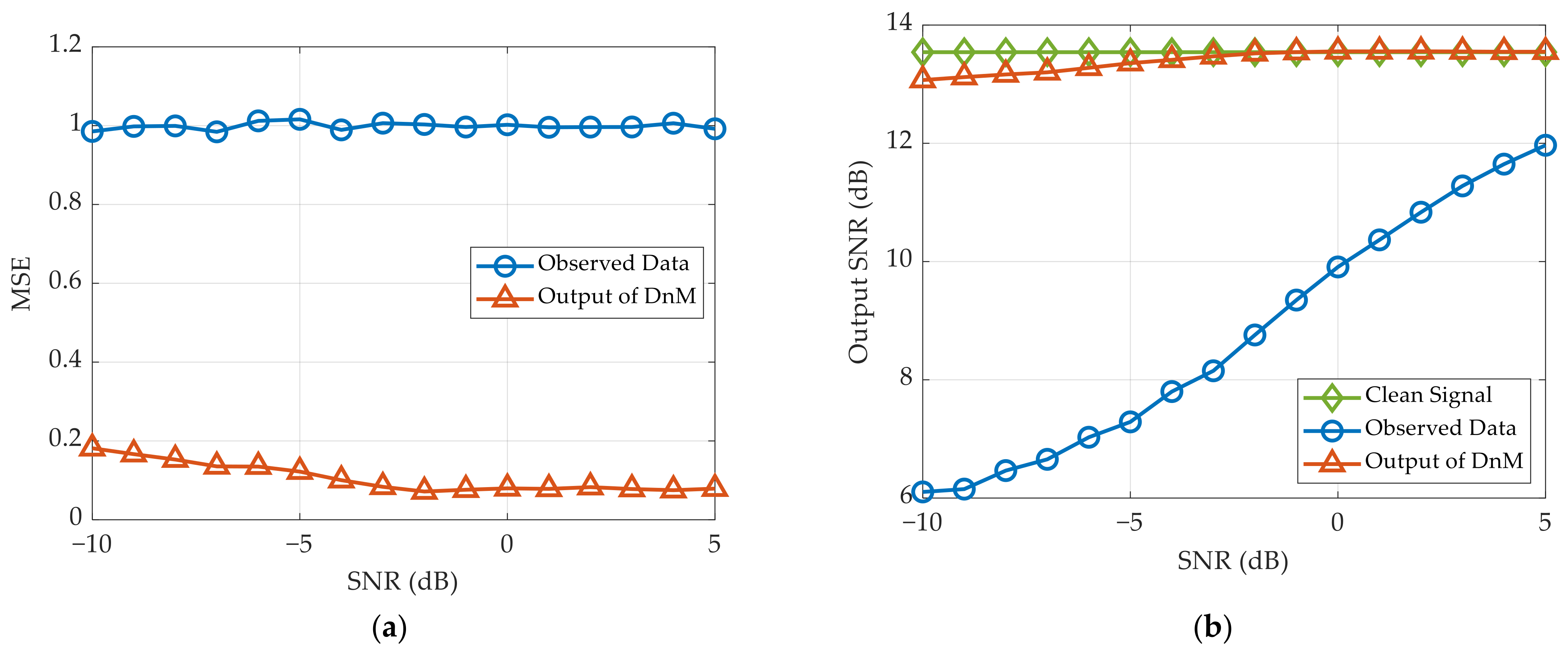
We assess the denoising performance through the MSE and output SNR in the scenario of one target. The simulation results with 1000 times Monte Carlo are displayed in Figure 8.

Figure 8a shows that the MSE using proposed network is stable under different SNRs. This means that the LDnADMM-Net can remove the high noise in the observed data effectively. Further, in Figure 8b, the output SNR after denoising enhances significantly in low SNR, which is close to the theoretical value of clean signal. Due to the high sidelobes caused by the NULA configuration, the theoretical output SNR is equivalent to the signal-to-sidelobe ratio. Therefore, the output SNR through DnM has converged to the theoretical value in high SNR, but its improvement is not significant.

5.2.2. Performance for DOA Estimations

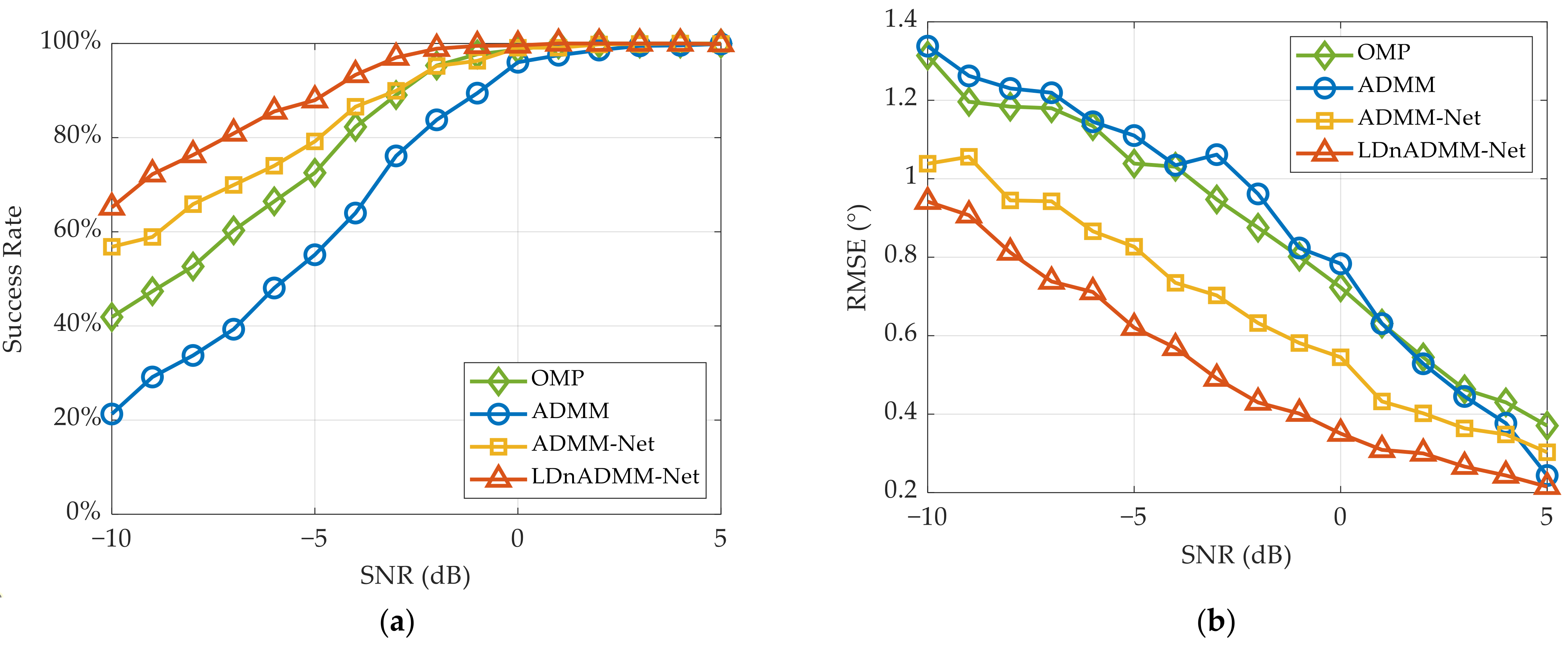
Using the above testing dataset, the DOA estimation results of different methods are presented in Figure 9, including the SR and RMSE.

As shown in Figure 9a, the success rate of DOA estimations through the LDnADMM-Net is noticeably superior to that of other methods, especially in a low SNR. Compared with the ADMM and ADMM-Net, the SR through the LDnADMM-Net at a low SNR can be increased by approximately 40% and 12%, respectively. This can be attributed to the use of a DnM that removes the strong noise from the observed data. By adaptively learning the parameters during the iterative process, the ADMM-Net can improve the success rate compared with the ADMM. Moreover, the LDnADMM-Net can obtain a further improvement by combining the DnM with the ADMM-Net.

Figure 9b demonstrates that the LDnADMM-Net also outperforms the other methods in terms of the DOA estimation accuracy. As the target SNR increases, the DOA estimation accuracy of all the methods can be enhanced. Compared with the OMP, ADMM and ADMM-Net, the RMSE of the LDnADMM-Net can be improved by approximately 0.4°, 0.4°, and 0.2°, respectively.

5.3. Simulation Results of Two Targets

According to the DOA interval and the SNR of two targets, two testing datasets are constructed to evaluate the performance of the LDnADMM-Net in the scenario of two targets.

Two targets with the same SNR = 0 dB are considered in the first testing dataset. The DOA value of the first target is selected randomly from −6° to 0°, and the other one adds a fixed DOA interval. The interval varies from 1° to 6°, and 1000 samples are generated for each interval.

In the second testing dataset, the DOA value of the first target is selected randomly from −6° to 0°, and the DOA interval between the two targets is fixed to 4°. These two targets are set to the same SNR, which is traversed from −10 dB to 5 dB with an interval of 1 dB. Similarly, 1000 samples are generated for each SNR.

5.3.1. Performance for Signal Denoising

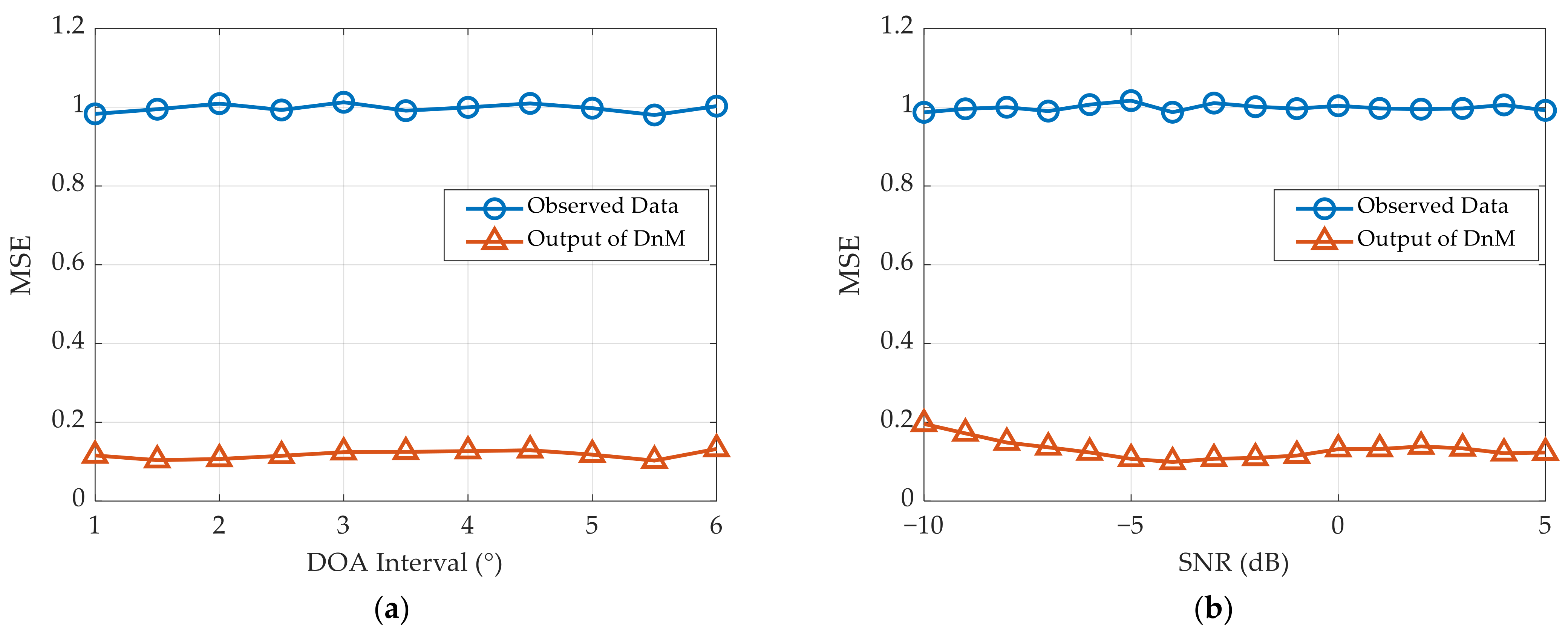
Using these two testing datasets, we first evaluate the denoising performance of the proposed network. Specifically, the simulation results with respect to the MSE are illustrated in Figure 10.

It is apparent that the observed data processed by the DnM in the proposed network are close to those processed by the clean signal. In the cases of different DOA intervals or target SNRs, the MSE after denoising can converge stably to approximately 0.15. This proves that the LDnADMM-Net can effectively remove the noise and has strong robustness.

5.3.2. Performance for DOA Estimations

Furthermore, using the above testing datasets, we calculate the PoR and RMSE to compare the DOA estimation performance of different methods.

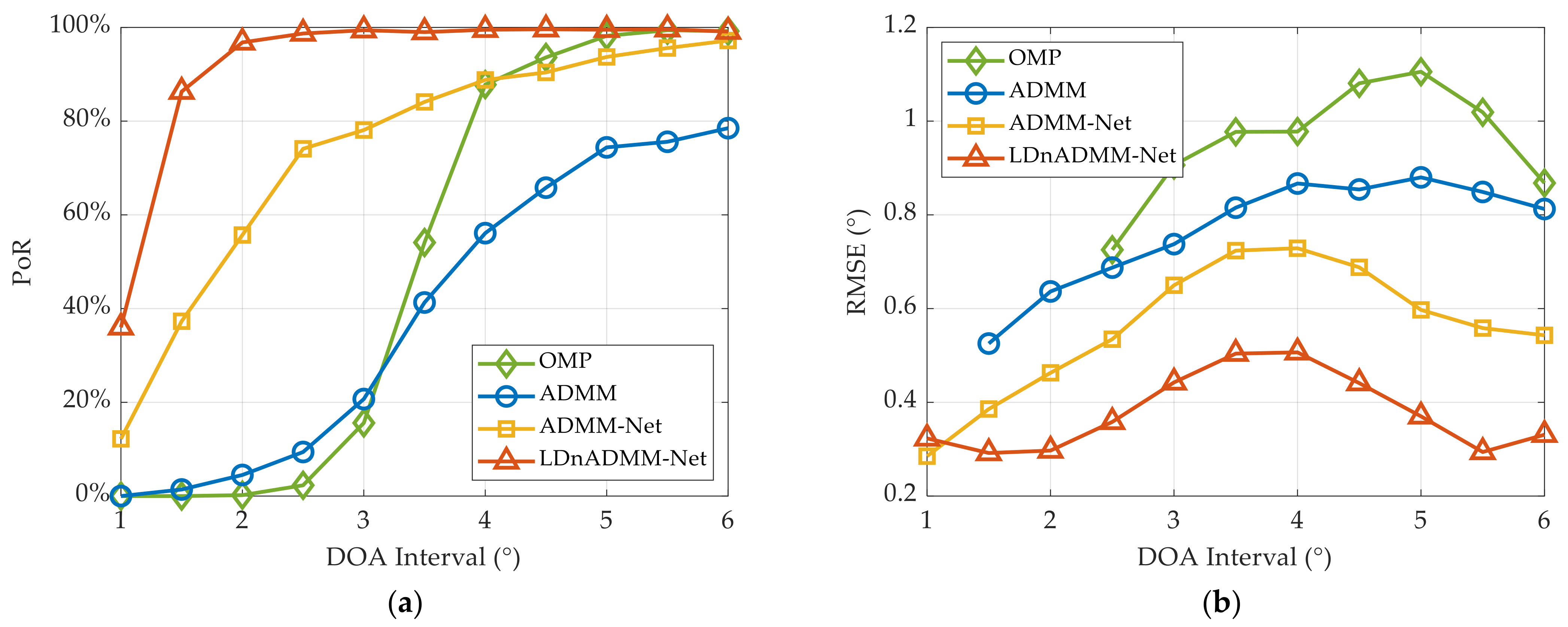
First, as illustrated in Figure 11a, we analyze the PoR results in the case of two targets with different DOA intervals. It can be found that the PoR results of all the methods are improved as the DOA interval increases. The OMP and ADMM methods decline significantly with a small DOA interval, while their performance can be improved when the DOA higher is larger than 3.5°. The ADMM-Net can be used to address this issue; however, it is still unsatisfactory for a high DOA interval. In contrast, the LDnADMM-Net reaches a 2° resolution with >95% probability. This means that the proposed network can achieve high super-resolution DOA estimations.

Then, Figure 11b demonstrates the RMSE results versus the DOA interval of different methods. The RMSE results are fluctuating, yet they demonstrate a stable trend. They specifically show fluctuations that increase and then decrease as the DOA interval increases. The reason for the fluctuations is that we do not use all the samples to calculate the RMSE. As mentioned in 5.1.3, we only counted the RMSE under a successful DOA estimation, i.e., the sample is required to satisfy the indicator’s PoR. According to the definition of the PoR, a successful resolution of two targets with a small DOA interval means a high estimation accuracy. On the other hand, these methods can distinguish the two targets well when the DOA interval exceeds 4°. In this case, the estimation accuracy of these methods can be improved as the DOA interval increases. Moreover, the RMSE results of the OMP, ADMM and ADMM-Net are approximately 1.0°, 0.8°, and 0.6°. Correspondingly, the RMSE of the LDnADMM-Net can be improved to approximately 0.4°.

Thereafter, using the second testing dataset, we compare the PoR of various methods versus that of the target SNR. The simulation results are displayed in Figure 12a. Obviously, the PoR results of all the methods are enhanced significantly as the SNR increases. The LDnADMM-Net is superior to the other methods, especially in a low SNR. Additionally, the proposed network can achieve the resolution with 100% probability at the SNR of > −2 dB. This further proves that the LDnADMM-Net can obtain a favorable anti-noise performance.

Finally, the RMSE results versus those of the target SNR are shown in Figure 12b. Compared with the OMP, ADMM, and ADMM-Net, the proposed network can improve the estimation accuracy by approximately 0.5°, 0.3°, and 0.2° with different SNRs.

6. Experimental Results

To further validate the effectiveness of our methods, real data experiments in an anechoic chamber are conducted in this section. We employ a radar prototype with a NULA configuration in the experiments. This NULA consists of three transmitting antennas and four receiving antennas, and the formed virtual arrays are consistent with the simulations.

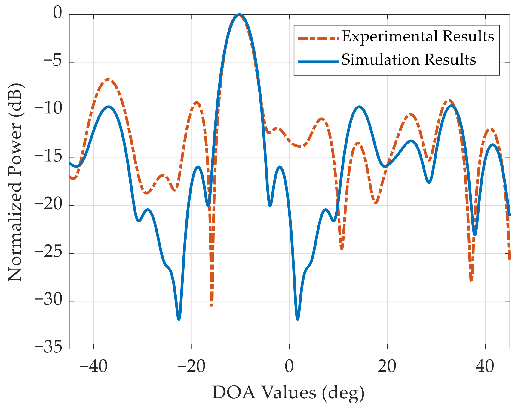
We carry out the amplitude-phase calibration for this NULA before the experiments. The antenna pattern after calibration is displayed in Figure 13. The antenna pattern is basically consistent with the simulation results, which proves the effectiveness and accuracy of the amplitude-phase calibration. Nevertheless, due to imperfect factors such as an array antenna position error, the peak sidelobe in the experiment increases to −6.8 dB.

6.1. Experiments of One Target

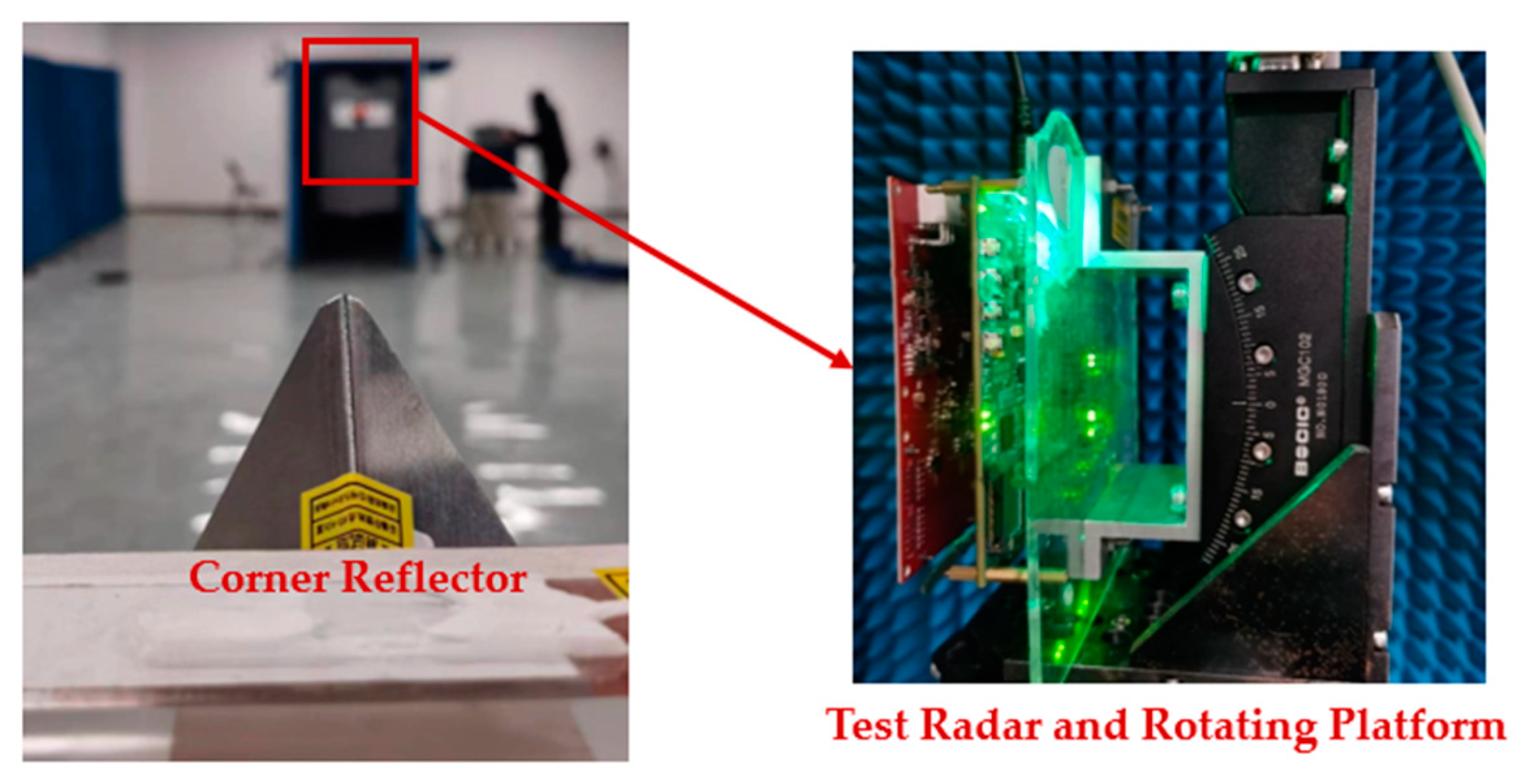
As shown in Figure 14, the radar prototype is mounted on a rotating platform in the anechoic chamber, and we place a 0 dBsm corner reflector as the target. We utilize the echoes of this corner reflector after range-Doppler matched filtering as the input data. It should be noted that the SNR of the input data can be calculated as an approximate of 2 dB. Since the spatial accumulation gain of the 12 antennas is about 11 dB, the output SNR can be approximated as 13 dB, which is close to the minimum detectable threshold used in practical applications.

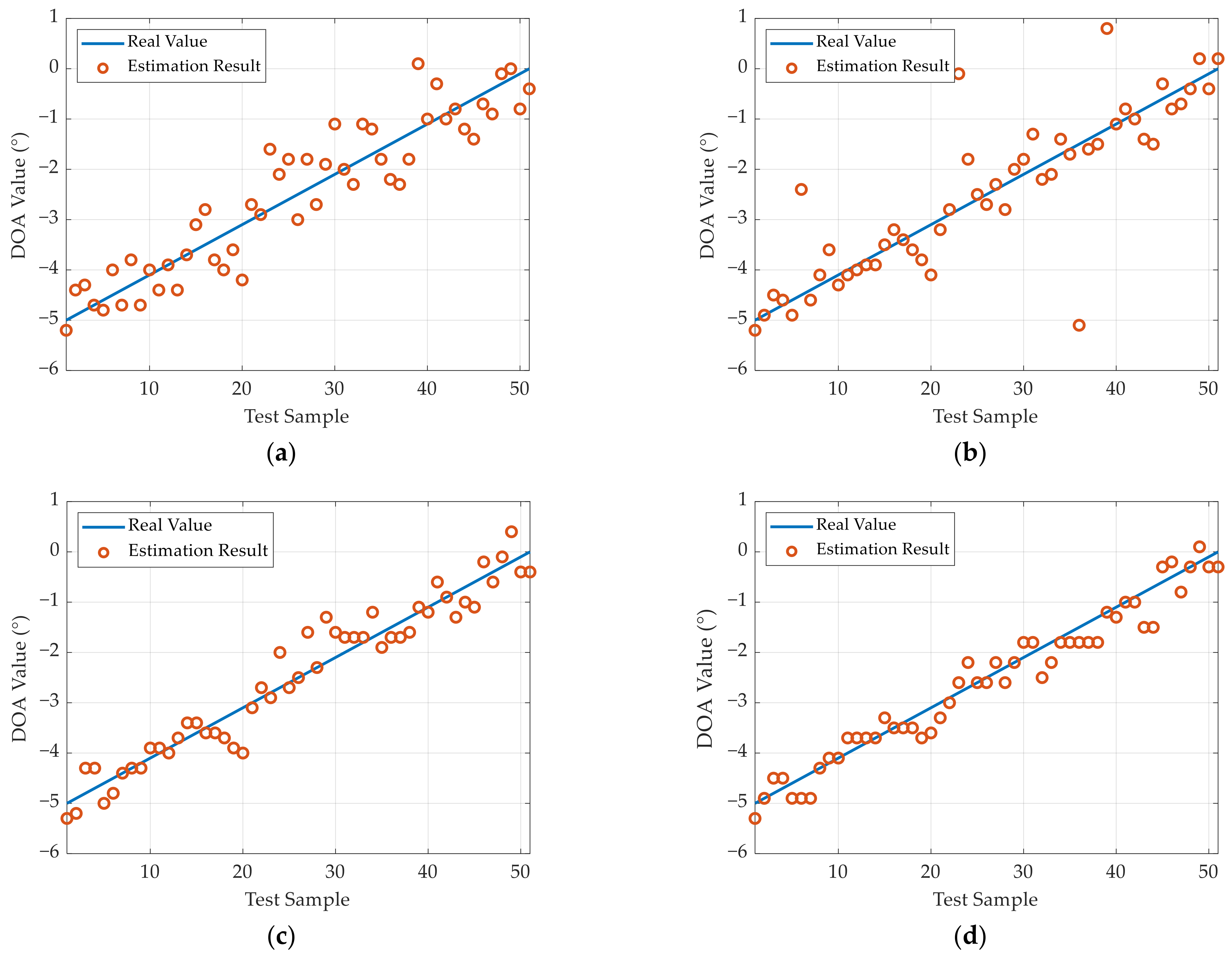
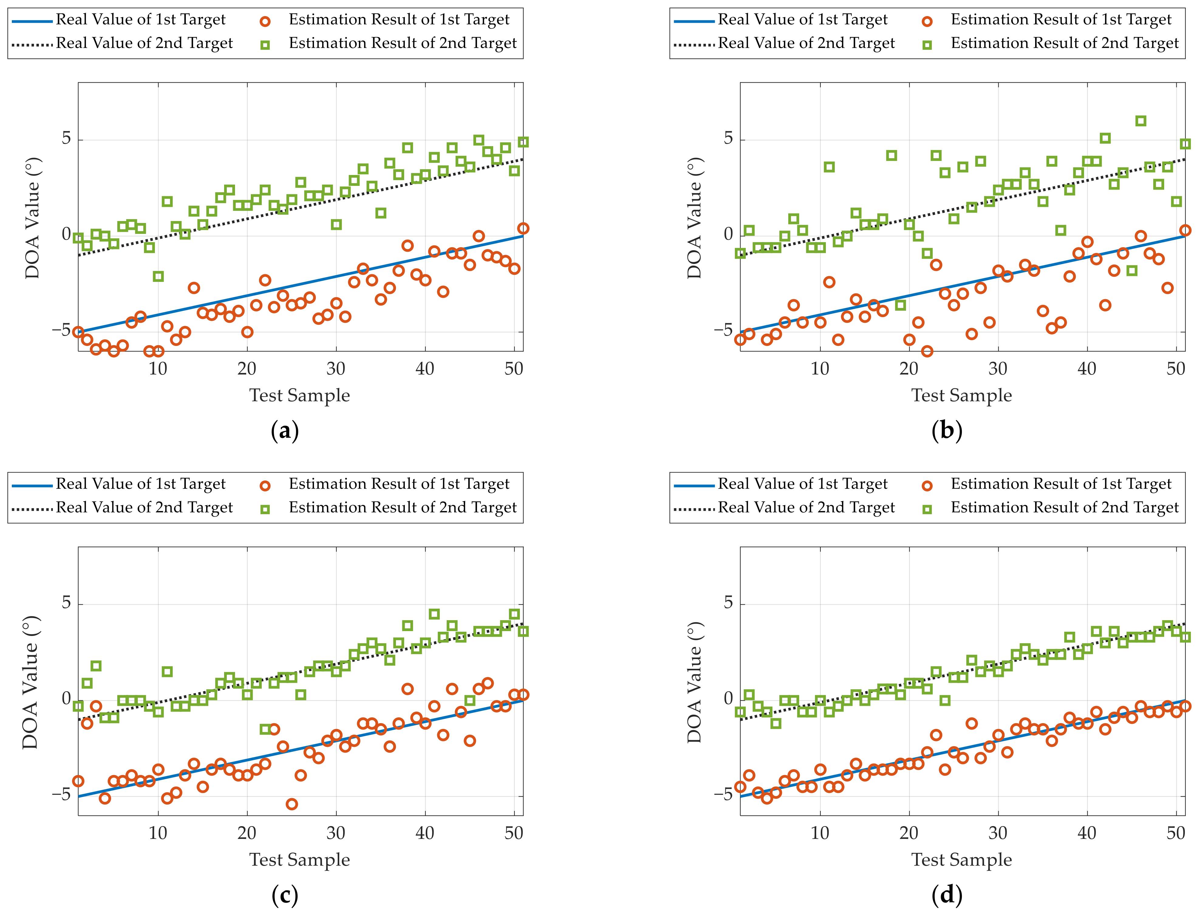
During experiments, the initial DOA value of the target is set to 0°. Using the rotating platform, the radar rotates to −5° and then gradually rotates to 0°. For each interval, we collected one set of data for testing. The experimental results are presented in Figure 15, and the SR and RMSE results of the different methods are given in

Table 5. The SR and the RMSE of the different methods in the scenario of one target.

Method	SR	RMSE
OMP	100%	0.4588°
ADMM	96.08%	0.4627°
ADMM-Net	100%	0.2961°
LDnADMM-Net	100%	0.2471°

.

It can be observed that the SR of all the methods is close to or reaches 100% in this test. In terms of the DOA estimation accuracy, the proposed method can achieve the optimal results. Referring to Table 5, the RMSE through the LDnADMM-Net can be improved by approximately 0.21°, 0.22°, and 0.05° compared with the other methods.

6.2. Experiments of Two Targets Separated by 2°

In this subsection, the initial DOAs of two targets (0 dBsm corner reflector) are set to 0° and −2°, respectively. Using the rotating platform, the radar rotates to −5° and then gradually rotates to 0° with an interval of 0.1°.

For each DOA interval, we collected one set of data for testing. The experimental results are demonstrated in Figure 16, and the PoR and RMSE results of the different methods are given in

Table 6. The PoR and the RMSE of different methods in the scenario of two targets separated by 2°.

Method	PoR	RMSE
OMP	0%	/
ADMM	1.96%	0.5585°
ADMM-Net	58.82%	0.4584°
LDnADMM-Net	98.04%	0.2830°

.

In this scenario where the two targets are separated by 2°, the proposed network clearly outperforms the other methods. This means that the LDnADMM-Net can obtain a stable super-resolution and high-accuracy estimation performance.

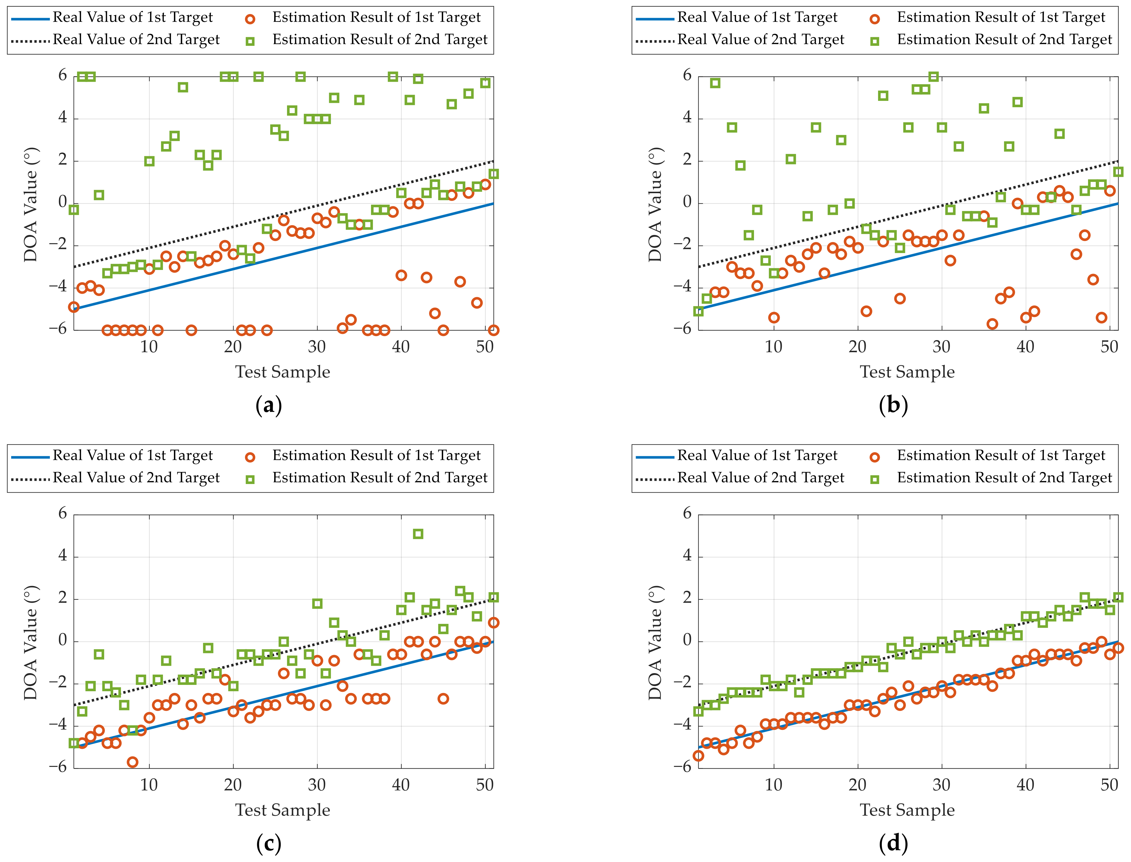
6.3. Experiments of Two Targets Separated by 4°

In this subsection, the initial DOAs of two targets (0 dBsm corner reflector) are set to 0° and −4°, respectively. Similarly, the radar rotates to −5° and then gradually rotates to 0°. For each DOA interval, we collected one set of data for testing. The experimental results are demonstrated in Figure 17, and the PoR and RMSE results of different methods are given in

Table 7. The PoR and the RMSE of different methods in the scenario of two targets separated by 4°.

Method	PoR	RMSE
OMP	88.24%	0.9364°
ADMM	56.86%	0.5827°
ADMM-Net	90.20%	0.5037°
LDnADMM-Net	100%	0.3240°

.

The experimental results show that the LDnADMM-Net can reach the resolution with 100% probability for two targets separated by 4°, which is significantly improved compared with the other methods. Moreover, the DOA estimation accuracy is also superior to that of the other methods. Referring to Table 7, it can improve by 0.61°, 0.26°, and 0.18°, compared with the OMP, ADMM, and ADMM-Net.

7. Conclusions

In this paper, we propose the LDnADMM-Net for DOA estimations in a non-uniform linear array under strong noise. The proposed network is designed by mapping the iterative processing of the ADMM into an unfolded deep neural network. In this way, the parameters in the ADMM can be transformed into the learnable network weights, and we can optimize them through network training. Moreover, to enhance the anti-noise performance of this network, we integrate the denoising convolutional neural network into each iteration.

Extensive simulations and experiments are carried out to verify the effectiveness of the proposed network. The simulations and experimental results demonstrate that the LDnADMM-Net can effectively improve the DOA estimation accuracy in the NULA configuration and provide a robust, super-resolution capability for multi-target scenarios.