A Full-Scale Shadow Detection Network Based on Multiple Attention Mechanisms for Remote-Sensing Images

Abstract

Shadows degrade image quality and complicate interpretation, underscoring the importance of accurate shadow detection for many image analysis tasks. However, due to the complex backgrounds and variable shadow characteristics of remote sensing images (RSIs), existing methods often struggle with accurately detecting shadows of various scales and misclassifying dark, non-shaded areas as shadows. To address these issues, we proposed a comprehensive shadow detection network called MAMNet. Firstly, we proposed a multi-scale spatial channel attention fusion module, which extracted multi-scale features incorporating both spatial and channel information, allowing the model to flexibly adapt to shadows of different scales. Secondly, to address the issue of false detection in non-shadow areas, we introduced a criss-cross attention module, enabling non-shadow pixels to be compared with other shadow and non-shadow pixels in the same row and column, learning similar features of pixels in the same category, which improved the classification accuracy of non-shadow pixels. Finally, to address the issue of important information from the other two modules being lost due to continuous upsampling during the decoding phase, we proposed an auxiliary branch module to assist the main branch in decision-making, ensuring that the final output retained the key information from all stages. The experimental results demonstrated that the model outperformed the current state-of-the-art RSI shadow detection method on the aerial imagery dataset for shadow detection (AISD). The model achieved an overall accuracy (OA) of 97.50%, an $F_1$ score of 94.07%, an intersection over union (IOU) of 88.87%, a precision of 95.06%, and a BER of 4.05%, respectively. Additionally, visualization results indicated that our model could effectively detect shadows of various scales while avoiding false detection in non-shadow areas. Therefore, this model offers an efficient solution for shadow detection in aerial imagery.

1. Introduction

With the rapid development of remote-sensing technology, high-resolution remote-sensing images have become prevalent across various fields, such as land surveying, ocean remote sensing, military and police defense, and emergency command. However, the presence of shadows in most optical remote-sensing images poses a series of challenges to computer vision tasks, such as object detection [1] and tracking [2]. These shadows are typically caused by tall objects, such as buildings, trees, and bridges, which block sunlight and create dark areas behind them [3]. As the spatial resolution of remote-sensing images continues to improve, the impact of shadows has become increasingly significant [4,5,6,7,8]. Specifically, shadow occlusion makes it challenging to fully extract ground object features in shadows, with local features often disrupted, thereby affecting the accuracy of ground object detection [9,10]. Furthermore, ensuring the accuracy of shadow detection is essential before proceeding with shadow removal, as the precision of shadow detection directly influences the quality of the subsequent shadow removal process [11,12]. Additionally, shadows provide supplementary data that can be used for tasks such as height inversion and the 3D reconstruction of buildings [13,14]. By analyzing the characteristics and positions of shadows, researchers can more accurately estimate the height of objects, thereby improving the precision of their models. During the 3D reconstruction of buildings, shadow information can aid in identifying the shapes and structural features of objects, optimizing the reconstruction results. In conclusion, shadow detection in remote-sensing images is an indispensable preprocessing step for subsequent analytical tasks.

Recent years have witnessed the emergence of many excellent shadow detection methods, mainly divided into two categories: traditional methods and machine learning-based methods. Among them, traditional methods can be further divided into geometric-based methods and attribute-based methods [15,16,17]. Geometric-based methods rely on prior knowledge related to the scene and sensors [18,19,20] to construct geometric models for shadow detection within the scene. Although these methods often provide good shadow detection performance, they face significant challenges in practical applications, as obtaining accurate geometric parameters is often quite difficult and is constrained by complex environmental conditions and variable lighting scenarios. In contrast, attribute-based methods generally outperform geometric-based methods to some extent because they do not require prior information. These methods focus on specific shadow attributes in the image, typically employing threshold-based methods. Threshold-based methods segment the image into shadow and non-shadow regions by setting a threshold based on the visual differences in brightness, saturation, and other relevant attributes between the shadow and non-shadow areas [21,22]. This method typically involves two steps. First, the original image is transformed into a new feature space that is suitable for shadow detection [23]. Next, the bimodal distribution of the histogram is utilized to determine the threshold, effectively distinguishing between shadow and non-shadow regions [24]. While effective, this method does not fully leverage the spatial information among pixels, as it processes each pixel individually. As a result, it often struggles to differentiate between genuine shadow areas and simply dark regions. Machine learning-based methods approach shadow detection as a binary classification problem, often employing classic learning-based classifiers such as support vector machines (SVM) to distinguish between shaded and non-shaded areas in images [25]. Although these methods have achieved higher levels of automation in shadow detection, they can sometimes struggle with accuracy due to limitations in learning deep features. This can lead to difficulties in capturing the complex patterns and variations in shadow characteristics, ultimately affecting the overall effectiveness of the detection process.

In recent years, continuous advancements in deep learning have led to significant progress, particularly with convolutional neural networks (CNNs) [26,27,28]. These networks have excelled in various areas of image processing due to their ability to automatically extract target features and effectively utilize nonlinear representations of input image data. Shadow detection is commonly approached as a binary semantic segmentation problem, with classical networks such as FCN [29], UNet [30], Deeplab [31], and PSPNet [32] proving highly effective in remote sensing tasks, including cloud and cloud shadow detection. As a result, shadow detection methods based on deep learning have garnered increasing attention. Chen et al. [33] proposed a multi-task mean teacher model for semi-supervised shadow detection, which effectively leveraged unlabeled data while exploring the potential to learn multiple aspects of shadow information simultaneously (DLA-PSO). He et al. [34] proposed an adaptive unsupervised shadow detection method based on multichannel features, which can flexibly adapt to different scenes and accurately identify shadow regions (MTMT). Luo et al. [35] proposed the first remote sensing image shadow detection dataset, known as the aerial imagery dataset for shadow detection (AISD), along with a corresponding deeply supervised CNN for shadow detection (DSSDNet). Jin et al. [36] designed a network utilizing a global-spatial-context attention module (GSCA-UNet). Additionally, Luo et al. [37] proposed the edge-aware spatial pyramid network (ESPFNet), which combines edge detection methods with neural networks, specifically focusing on capturing shadow edge features. Zhu et al. [38] developed a contextual detail-aware network for shadow extraction (CDANet), demonstrating promising results. Liu et al. [39] presented the MSASDNet to tackle the challenge of distinguishing between illuminated and shaded areas, emphasizing its effectiveness in mitigating the influence of non-shaded regions. Zhang et al. [40] proposed a multi-scale shadow extraction method for remote-sensing images that incorporates clustering and detail features (DTHNet). Furthermore, Zhang et al. [41] developed a deep neural network named MRPFA-Net, which leverages multiresolution parallel fusion decoding and integrates cross-spatial and channel attention mechanisms for shadow detection in high-resolution remote-sensing images. Finally, Chen et al. [42] pioneered the integration of neural networks with distance transformation algorithms for shadow detection, introducing a novel approach called the slice-to-slice context transfer and uncertainty region calibration network (SCUCNet).

Although existing shadow detection networks have achieved significant results in processing remote-sensing images, most rely solely on spatial attention or multi-scale methods. The use of a single approach has limitations, often failing to fully exploit the deep features obtained during the decoding phase, leading to reduced detection accuracy when encountering multi-scale shadows. Furthermore, previous methods did not fully utilize pixel-wise relational information, making non-shadow areas prone to false detection. In addition, existing methods often overlook important channel information. The current challenges in shadow detection are summarized as follows:

(1)

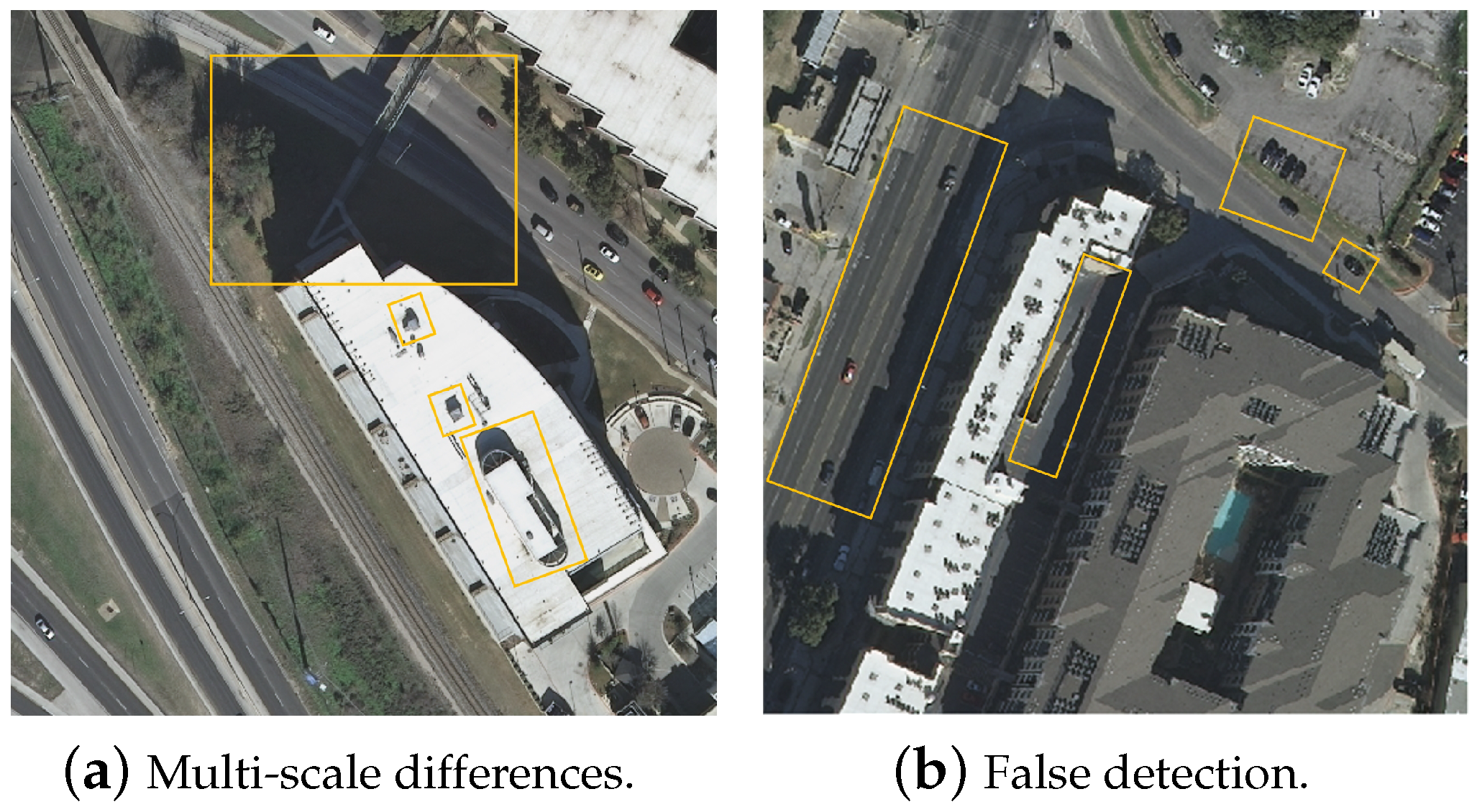
Decreased accuracy in shadow detection across different scales: As shown in Figure 1a, the varying scales and morphological features of different objects in the image result in diverse scale differences in shadows, thereby affecting the current network’s accuracy in shadow detection across different scales.

(2)

False detection in non-shadow regions: As shown in Figure 1b, the image contains some dark objects, such as cars and roads, whose spectral information and texture structures closely resemble shadows, thus easily leading to false detection as shadows.

To address the above two issues and improve shadow detection performance, we proposed MAMNet, a comprehensive shadow detection network integrating multiple attention mechanisms. The main contributions of this study are as follows:

(1)

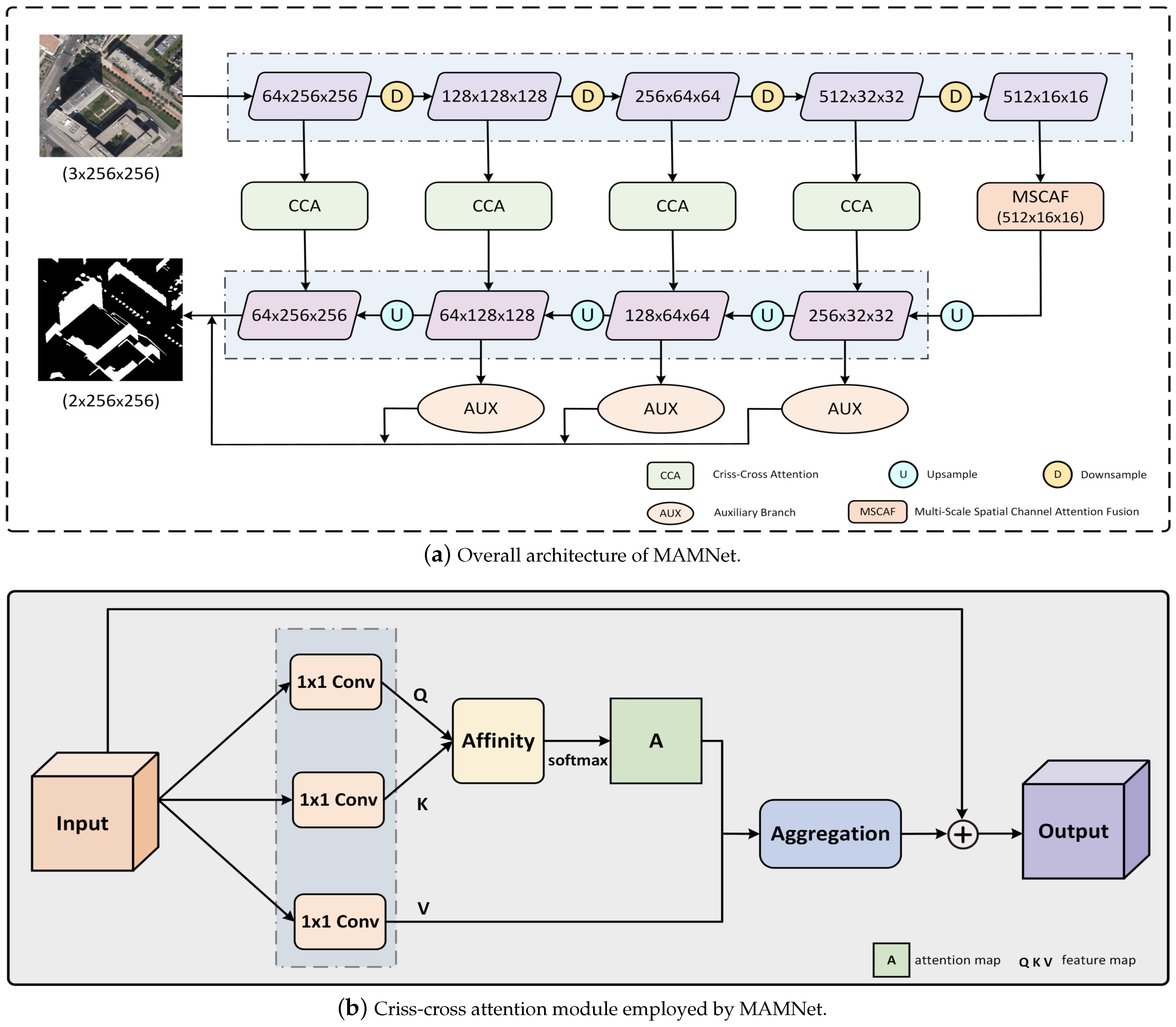
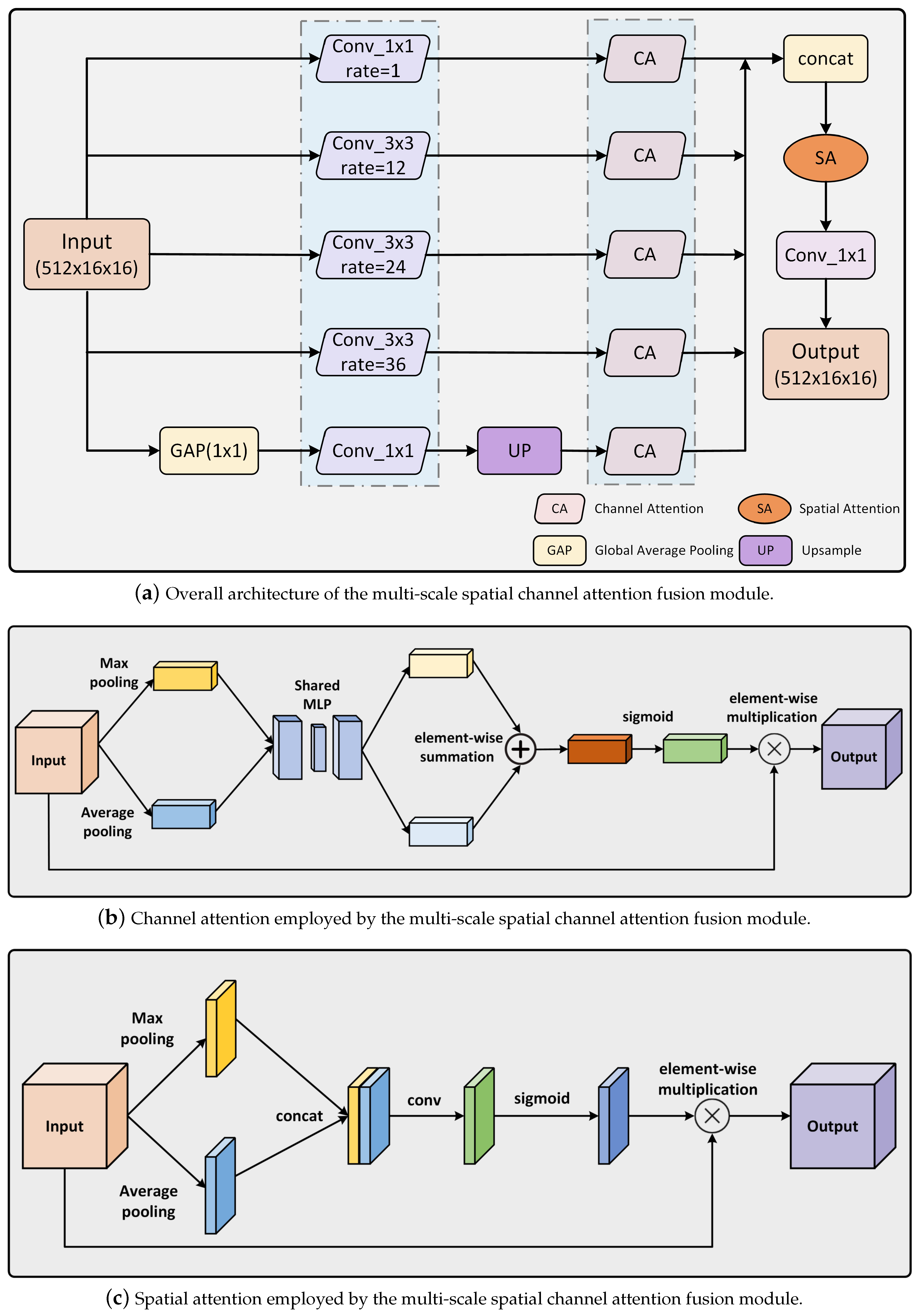
We proposed a multi-scale spatial channel attention fusion module that fully exploited the deep features extracted by the encoder, accurately capturing the shadow positions, shapes, and channel information across different scales in shadow images, enabling the model to handle shadows of various scales with greater flexibility and effectively reducing the impact of scale differences.

(2)

By introducing the criss-cross attention module, non-shadow pixels were compared with other shadow and non-shadow pixels in the same row and column, learning similar characteristics of pixels in the same category, which improved the classification accuracy of non-shadow pixels and avoided false detections in non-shadow areas.

(3)

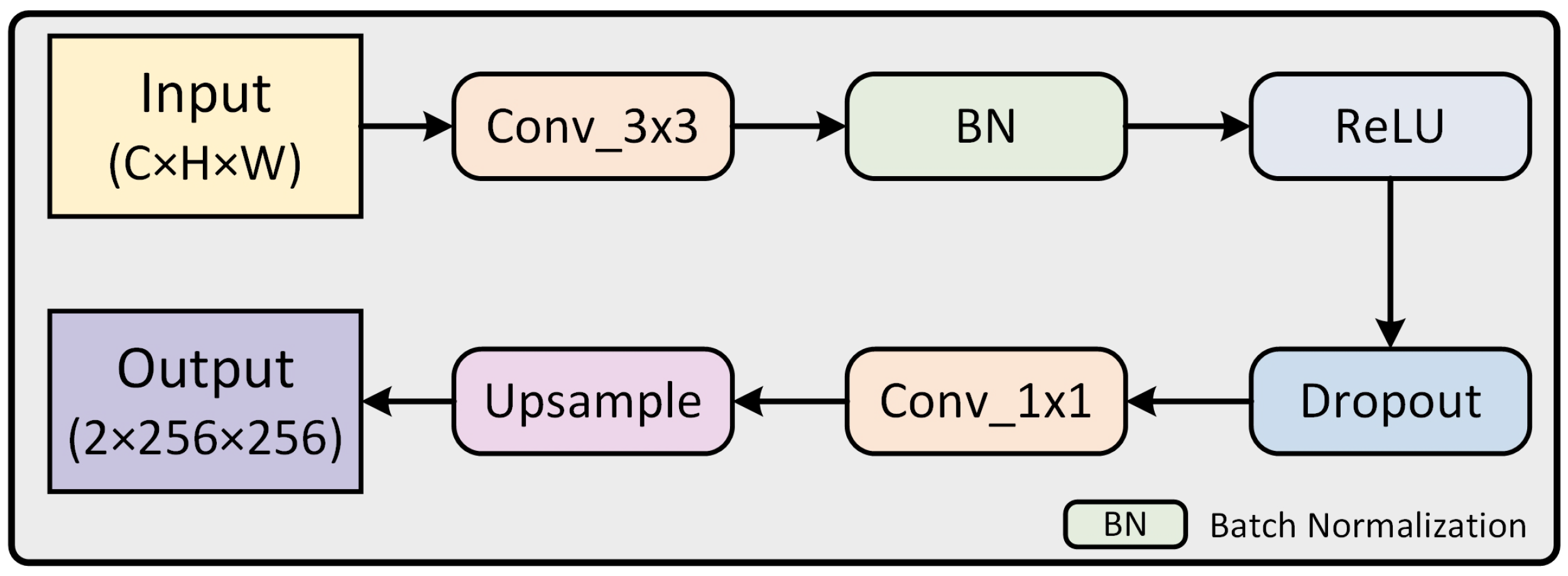
To address the issue of important information from the other two modules being lost due to continuous upsampling during the decoding phase, we proposed an auxiliary branch module to assist the main branch in decision-making, which ensured that the final output retained key information from all stages.

(4)

Experimental validation was conducted on the AISD dataset, showcasing the superior performance of MAMNet compared to existing state-of-the-art methods. Additionally, visualization results indicated that our model could effectively detect shadows of various scales while avoiding false detection in non-shadow areas.

2. Materials and Methods

2.1. Data Preprocessing

We trained our model with the publicly available AISD dataset [35], which can be obtained from https://github.com/RSrscoder/AISD, (accessed on 1 December 2023). The input data consist of shadow images in the .tif format and their corresponding labels, where the shadow images contain intensity values with no direct physical meaning and are 8-bit data, with pixel values ranging from 0 to 255. The labels are single-channel grayscale images used to represent classification indices, such as shadow and non-shadow regions. Before being fed into the network, the shadow images in the .tif format were preprocessed, with pixel values normalized to the [0, 1] range. In order to enhance the diversity of the dataset and reduce the risk of overfitting, we adopted an effective data augmentation technique that uniformly cropped the original images into small blocks of size 256 × 256 pixels. Through this method, we generated a total of 11,836 fixed-size patches, each containing rich spatial information and contributing to the enrichment of the training sample set for our model. The cropping process is meticulously designed to ensure complete coverage of the original image while selecting information-rich areas. It follows a specific strategy: we slide a window on the original image with dimensions of 256 × 256 pixels and a spacing of 64 pixels to ensure complete coverage of the original image while selecting information-rich areas. In particular, we focus on preserving areas with a sufficient number of shadow pixels, which helps the model better understand the details and structure of the image.

The entire process of shadow detection is shown in Figure 2. First, the preprocessed data are input into the proposed model for training, optimizing parameters through continuous iterations to obtain the optimal weights. After training is complete, the model will be used to predict images in the test set, accurately identifying shadow regions.

2.2. Method Overview

MAMNet adopts an encoder–decoder structure, where the entire shadow image serves as input, and the model outputs shadow detection images in an end-to-end manner. Figure 3a shows the structure of MAMNet, which mainly consists of three modules: a multi-scale spatial channel attention fusion module, a criss-cross attention module, and an auxiliary branch module. Specifically, the input image is first subjected to preliminary feature extraction through an encoder to obtain deep features. Then, these features are fed into the multi-scale spatial channel attention fusion module for additional refinement, yielding multi-scale feature maps enriched with both spatial and channel information. In the decoding stage, these multi-scale feature maps are gradually restored to their original resolution through continuous upsampling. At the same time, the model processes different resolution feature maps of each stage of the encoder through a criss-cross attention module to mitigate the risk of false detection. Then, the output from the criss-cross attention module is routed back to the corresponding stage of the decoder to refine the feature maps. In addition, the model combines the outputs of both the auxiliary and main branches to form the final prediction result. The specific implementation details of each module will be thoroughly covered in this section.

2.3. Multi-Scale Spatial Channel Attention Fusion Module

Existing models mostly rely on spatial attention or multi-scale methods, which have limitations and often fail to fully utilize the deep features obtained during the decoding phase, resulting in reduced detection accuracy in multi-scale shadow scenarios. Additionally, these methods often overlook important channel information. To address these issues, we proposed a multi-scale spatial channel attention fusion module (MSCAF), as shown in Figure 4a. This module thoroughly exploits the deep feature information extracted by the encoder, enabling accurate capture of shadow positions, shapes, and channel characteristics at different scales in shadow images. As a result, the model gains enhanced flexibility in handling shadows of various sizes and effectively mitigates the impact of multi-scale shadow differences. Specifically, the MSCAF module consists of five parallel branches, with four containing channel attention and dilated convolution. These branches utilize dilation rates of 1, 12, 24, and 36, respectively. The fifth branch includes global average pooling (GAP), upsampling layer (UP), and channel attention (CA). Following fusion, the resultant feature maps undergo input into a spatial attention (SA) mechanism to enhance the model’s correlation and importance of features at different spatial positions, directing the model’s attention towards shadows in the image, effectively improving precision in identifying and delineating shadow regions, thus enhancing the overall detection performance. Finally, a 3 × 3 convolutional layer is applied, serving to reduce the number of output channels.

There are many multichannel feature maps in the network, with some channels potentially better suited for capturing shadow-related features while others excel in representing non-shadow areas. In order to optimize the shadow detection task, we introduced a channel attention module to filter feature channels, emphasizing the features of shadow areas, thereby enhancing the network’s perception of shadows and improving the accuracy of shadow detection. The structure of the channel attention structure is shown in Figure 4b. The overall channel attention process is summarized as follows:

$${\mathbf{F}}^{\prime }={\mathbf{M}}_{\mathbf{c}}\left(\mathbf{F}\right)\otimes \mathbf{F},$$

(1)

where $\mathbf{F}\in R^{C\times W\times H}$ is the input feature map, ⊗ denotes element-wise multiplication, ${\mathbf{F}}^{\prime }$ denotes the output feature map, and ${\mathbf{M}}_{\mathbf{c}}\left(\mathbf{F}\right)$ represents the channel attention weight.

Among them, the channel attention weight is obtained through the following steps. Firstly, we perform average-pooling and max-pooling operations on the input feature map $\mathbf{F}$. These operations aggregate spatial information to obtain two (C × 1 × 1) feature maps. Then, each of these two feature maps passes through a shared two-layer neural network. This shared network consists of multi-layer perceptrons ($MLP$) with a hidden layer. The first layer of $MLP$ contains ${\displaystyle \frac{C}{r}}$ neurons, where r is the reduction rate. The second layer contains C neurons. Following the processing through the shared $MLP$, we conduct an element-wise summation of the feature vectors output by $MLP$. This summation generates the final channel attention weight ${\mathbf{M}}_{\mathbf{c}}\left(\mathbf{F}\right)$ through the sigmoid activation function. ${\mathbf{M}}_{\mathbf{c}}\left(\mathbf{F}\right)$ can be computed as follows:

$$\begin{array}{cc}\hfill {\mathbf{M}}_{\mathbf{c}}\left(\mathbf{F}\right)& =\sigma (MLP(AvgPool(\mathbf{F}))+MLP(MaxPool(\mathbf{F})))\hfill \\ \hfill & =\sigma ({\mathbf{W}}_{\mathbf{1}}({\mathbf{W}}_{\mathbf{0}}({\mathbf{F}}_{\mathbf{avg}}^{\mathbf{c}}))+{\mathbf{W}}_{\mathbf{1}}({\mathbf{W}}_{\mathbf{0}}({\mathbf{F}}_{\mathbf{max}}^{\mathbf{c}}))),\hfill \end{array}$$

(2)

where $\sigma$ denotes the sigmoid function, ${\mathbf{W}}_{\mathbf{0}}\in R^{\frac{C}{r}\times C}$, and ${\mathbf{W}}_{\mathbf{1}}\in R^{C\times \frac{C}{r}}$.

Integrating a spatial attention mechanism into neural networks proves to be a powerful strategy to enhance the neural network’s ability to discern shadow positions and shapes in images. This mechanism empowers the network to selectively focus on different regions of the image, particularly those possibly containing shadows, thus significantly improving the accuracy and robustness of shadow detection algorithms. The structure of spatial attention is shown in Figure 4c. The overall spatial attention process can be expressed as follows:

$${\mathbf{F}}^{\prime }={\mathbf{M}}_{\mathbf{s}}\left(\mathbf{F}\right)\otimes \mathbf{F},$$

(3)

where $\mathbf{F}\in R^{C\times W\times H}$ denotes the input feature map, ⊗ denotes element-wise multiplication, ${\mathbf{F}}^{\prime }$ denotes the output feature map, and ${\mathbf{M}}_{\mathbf{s}}\left(\mathbf{F}\right)$ represents the spatial attention weight.

Among them, the spatial attention weight is obtained through the following steps. Firstly, we conduct average-pooling and max-pooling operations on the input feature map $\mathbf{F}$. These operations aggregate the channel information of the feature map and obtain two (1 × H × W) feature maps. Then, the two feature maps are concatenated based on their channels. Subsequently, a 7 × 7 convolution operation is performed, reducing the number of channels to 1 and resulting in a (1 × H × W) feature map. Finally, the spatial attention weight ${\mathbf{M}}_{\mathbf{s}}\left(\mathbf{F}\right)$ is generated using the sigmoid function. ${\mathbf{M}}_{\mathbf{s}}\left(\mathbf{F}\right)$ can be computed as follows:

$$\begin{array}{cc}\hfill {\mathbf{M}}_{\mathbf{s}}\left(\mathbf{F}\right)& =\sigma (f^{7\times 7}([AvgPool(\mathbf{F}); MaxPool(\mathbf{F})]))\hfill \\ \hfill & =\sigma (f^{7\times 7}([{\mathbf{F}}_{\mathbf{avg}}^{\mathbf{s}}; {\mathbf{F}}_{\mathbf{max}}^{\mathbf{s}}])),\hfill \end{array}$$

(4)

where $\sigma$ denotes the sigmoid function, and $f^{7\times 7}$ represents a convolution operation with a filter size of 7 × 7.

In conclusion, by introducing the multi-scale spatial channel attention fusion module, the model is able to accurately capture the shadow positions, shapes, and channel information across different scales in shadow images. This enhances the model’s ability to handle shadows of various scales, making it more flexible in dealing with scale differences and effectively reducing the impact of scale variation.

2.4. Criss-Cross Attention Module

Previous methods often resulted in false detection in non-shadow areas due to the failure to fully leverage the spatial relationships between pixels. These methods overlooked the contextual information between pixels, making it difficult for the model to distinguish subtle differences between shadow and non-shadow regions. To address this issue, a criss-cross attention module [43] was introduced. Comparing non-shadow pixels with other shadow and non-shadow pixels in the same row and column enhances the learning of similar features between pixels. This module enables the model to capture the similarity of pixels within the same class, thereby improving the classification accuracy of non-shadow pixels and effectively preventing false detection in non-shadow areas.

As shown in Figure 3b, the input to the module consists of local feature map $\mathbf{F}\in R^{C\times W\times H}$, which undergoes dimension reduction via 1 × 1 convolution to yield two feature maps $\mathbf{Q}\in R^{C^{\prime }\times W\times H}$ and $\mathbf{K}\in R^{C^{\prime }\times W\times H}$. At each position $\mathbf{u}$ in the spatial dimension of feature map $\mathbf{Q}$, we can obtain a vector ${\mathbf{Q}}_{\mathbf{u}}$. We can also obtain the set ${\mathbf{\Omega }}_{\mathbf{u}}\in R^{(H+W-1)\times C^{\prime }}$ by extracting feature vectors from K, which are in the same row or column as position $\mathbf{u}$. The affinity operation can be obtained from Formula (5):

$${\mathbf{d}}_{\mathbf{i},\mathbf{u}}={\mathbf{Q}}_{\mathbf{u}}{\mathbf{\Omega }}_{\mathbf{i},\mathbf{u}}^{\mathbf{T}},$$

(5)

where ${\mathbf{\Omega }}_{\mathbf{i},\mathbf{u}}$ denotes the ith element of ${\mathbf{\Omega }}_{\mathbf{u}}$, and ${\mathbf{d}}_{\mathbf{i},\mathbf{u}}\in D$ denotes the degree of correlation between feature ${\mathbf{Q}}_{\mathbf{u}}$ and ${\mathbf{\Omega }}_{\mathbf{i},\mathbf{u}}$.

After the affinity operation of each element for ${\mathbf{\Omega }}_{\mathbf{u}}$, an attention map $\mathbf{A}\in R^{(H+W-1)\times W\times H}$ is obtained through a softmax layer. Afterwards, by applying a 1 × 1 convolution to the local feature map $\mathbf{F}$, the feature map $\mathbf{V}\in R^{C\times W\times H}$ can be obtained. At each position $\mathbf{u}$ in the spatial dimension of feature map $\mathbf{V}$, we can obtain a vector ${\mathbf{V}}_{\mathbf{u}}\in R^C$ and a set ${\mathbf{\Phi }}_{\mathbf{u}}\in R^{(H+W-1)\times C}$. More powerful feature maps ${\mathbf{F}}_{\mathbf{u}}^{\prime }$ are obtained by the aggregation operation, as shown in Formula (6):

$${\mathbf{F}}_{\mathbf{u}}^{\prime }={\mathbf{\Sigma }}_{\mathbf{i}\in \mid {\mathbf{\Phi }}_{\mathbf{u}}\mid }{\mathbf{A}}_{\mathbf{i},\mathbf{u}}{\mathbf{\Phi }}_{\mathbf{i},\mathbf{u}}+{\mathbf{F}}_{\mathbf{u}},$$

(6)

where ${\mathbf{F}}_{\mathbf{u}}^{\prime }$ is a feature vector in the output feature map ${\mathbf{F}}^{\prime }\in R^{C\times W\times H}$ at position $\mathbf{u}$. The set ${\mathbf{\Phi }}_{\mathbf{u}}$ denotes a collection of feature vectors in $\mathbf{V}$, which are in the same row or column as position $\mathbf{u}$. ${\mathbf{A}}_{\mathbf{i},\mathbf{u}}$ is a scalar value at channel $\mathbf{i}$ and position $\mathbf{u}$ in $\mathbf{A}$.

Through the operations above, the context information is added to the local feature map $\mathbf{F}$ to enrich the pixel-wise representation so that the model can better distinguish the subtle differences between shadow and non-shadow pixels.

2.5. Auxiliary Branch Module

During the decoding stage, continuous upsampling resulted in the loss of important information, and relying solely on a single main branch weakened the effectiveness of the MSCAF and CCA modules we proposed. To address this, we introduced an auxiliary branch module to assist the main branch in decision-making, allowing the final output to integrate information from all stages, thereby fully leveraging the capabilities of these two modules. In addition, since shadow detection is a binary classification problem, the number of output channels of both the auxiliary branch and the main branch is the same, which is 2. As shown in Figure 3a, our auxiliary branch module (AUX) consists of three auxiliary branches designed to support the main branch in shadow detection. Specifically, in the processing of the model, each auxiliary branch employs a sequence of operations. As can be seen in Figure 5, it starts with a 3 × 3 convolutional layer to extract features, followed by a batch normalization (BN) layer to normalize the features and a rectified linear unit (ReLU) activation function layer to introduce non-linearity. Subsequently, a dropout layer is applied to mitigate overfitting and eliminate unnecessary information. Following the feature extraction process, the prediction results from each auxiliary branch are output through a 1 × 1 convolutional layer. These results are then amplified to the original size through an upsampling layer to match the dimensions of the input image. Finally, the prediction results of each auxiliary branch are fused with the output results of the main branch of the model to obtain the final prediction result containing information from each stage, which further improves the detection accuracy.

3. Experiments and Analysis

In this section, we begin by introducing the dataset utilized in our experiments. Additionally, we provide details regarding the experimental setup, including the selection of appropriate loss functions and the evaluation metrics used to assess the performance of the model. Next, we conducted quantitative comparisons against other algorithms through experiments and conducted ablation experiments to verify the individual contributions and effectiveness of each design module within our model architecture. Finally, we conducted a visual analysis of the experimental results to gain a deeper understanding of the performance and behavior of the model.

3.1. Dataset and Implementation Details

Experimental Dataset: Our proposed method is trained, validated, and tested on the open AISD dataset [35], which includes 514 images along with their corresponding labels. Specifically, 412 images are allocated for training purposes, while both the validation and testing sets consist of 51 images each. The remote sensing images in the dataset contain three bands: red, green, and blue, corresponding to the following wavelength ranges: red band (620 nm to 750 nm), green band (495 nm to 570 nm), and blue band (450 nm to 495 nm). The spatial resolution of the AISD dataset is 0.3 m per pixel. The pixel size of the images ranges from 256 × 256 pixels (corresponding to a ground coverage of 76.8 m × 76.8 m) to 1688 × 1688 pixels (corresponding to a ground coverage of 506.4 m × 506.4 m). This dataset covers aerial remote sensing shadow images from five regions: Austin, Chicago, Innsbruck, Tyrol, and Vienna. As can be seen in Figure 6, it can be observed that there are significant differences in urban structure among different regions. For example, Austin and Chicago are commercial cities with dense skyscrapers casting distinct shadows. Innsbruck is characterized by low and dense buildings, while Tyrol presents low and sparse buildings surrounded by a wide range of trees. Vienna presents a closed circular structure with a large number of trees planted inside. This diversity enriches the content of the dataset and facilitates the training of robust models. In addition, shadows in the dataset are mainly composed of buildings and vegetation, presenting different morphological characteristics. The shadows cast by buildings typically exhibit regular shapes and cover large areas, while the shadows of vegetation show an irregular, scattered distribution. Therefore, one of the challenges encountered in this study of remote sensing shadow detection is appropriately addressing the differences in shadow characteristics at different scales.

Experimental Setting and Loss Function: In the experimental setup, we set the learning rate of the model to 0.001 and used the Adam optimizer to optimize the network parameters in accordance with the hyperparameter settings from reference [39]. Cross-entropy loss served as the loss function for training the model. The network training spanned 15 epochs, during which the proposed network was implemented under the PyTorch framework. The training process was executed on a GeForce RTX3080. Due to memory limitations, we have set the size of the minibatch to 4. The expression for the cross-entropy loss function is as follows:

$$L=-\left[\mathrm{y}\log \right(\mathit{p})+(1-\mathrm{y}\left)\log \right(1-\mathit{p}\left)\right].$$

(7)

Among them, $\mathrm{y}$ represents the label of the sample, with positive classes assigned a value of 1, indicating the presence of the feature of interest, such as shadows, while negative classes are assigned a value of 0, signifying the absence of that feature. Meanwhile, $\mathit{p}$ denotes the probability that the predicted sample is positive.

Evaluation Metrics: The shadow detection results are comprehensively evaluated using overall accuracy (OA), precision, $F_1$ score, bit error rate (BER), and intersection over union (IOU). Among these metrics, higher values of OA, precision, $F_1$ score, and IOU signify better detection effectiveness. Conversely, a lower BER indicates superior detection performance. The calculation method for the five indicators is as follows:

$$\mathrm{OA}={\displaystyle \frac{\mathrm{TP}+\mathrm{TN}}{\mathrm{TP}+\mathrm{FP}+\mathrm{TN}+\mathrm{FN}}},$$

(8)

$$\mathrm{P}={\displaystyle \frac{\mathrm{TP}}{\mathrm{TP}+\mathrm{FP}}},$$

(9)

$$F_1={\displaystyle \frac{2\times \mathrm{TP}}{2\times \mathrm{TP}+\mathrm{FP}+\mathrm{FN}}},$$

(10)

$$\mathrm{BER}=1-{\displaystyle \frac{1}{2}}({\displaystyle \frac{\mathrm{TP}}{\mathrm{TP}+\mathrm{FN}}}+{\displaystyle \frac{\mathrm{TN}}{\mathrm{TN}+\mathrm{FP}}}),$$

(11)

$$\mathrm{IOU}={\displaystyle \frac{\mathrm{TP}}{\mathrm{TP}+\mathrm{FP}+\mathrm{FN}}},$$

(12)

where true positive (TP) refers to instances where both the real situation and the predicted result are shadows, true negative (TN) denotes cases where only the real situation is a shadow, yet the result is not correctly predicted as a shadow, false positive (FP) occurs when the real situation is not a shadow, but the result is incorrect as a shadow, and false negative (FN) signifies instances where both the real situation and the predicted result are not shadows.

3.2. Ablation Study

Ablation experiments with different settings were conducted to verify the contribution of each module. In order to better control the parameters for comparison, ablation experiments were conducted by modifying the network and removing individual modules, as shown in

Table 1. Quantitative evaluation of component ablation experiments.

Methods	OA (%)	Precision (%)	F1 Score (%)	BER (%)	IOU (%)
w/o MSCAF	97.28	93.45	93.55	3.99	87.95
w/o CCA	97.37	94.76	93.74	4.25	88.28
w/o AUX	97.20	93.32	93.41	4.07	87.72
MAMNet (Ours)	97.50	95.06	94.07	4.05	88.87

. Experiment 1: no MSCAF module; experiment 2: no CCA module; experiment 3: no AUX module; experiment 4: MAMNet. All four experiments were conducted under the same training conditions. Please note that the bold text is used to highlight the optimal experimental results.

Without MSCAF: Other structures remained unchanged in this experiment, with the network solely extracting deep features through an encoder without further processing. Due to the absence of multi-scale features containing spatial and channel information, there was a notable decrease in the values of OA, precision, $F_1$ score, and IOU by 0.22%, 1.61%, 0.52%, and 0.92%, respectively. This indicated that the model failed to fully utilize the deep features extracted by the encoder, making it difficult to capture positional, shape, and channel information of shadows at different scales. As a result, the model struggled to adapt flexibly to shadow detection across varying scales.

Without CCA: The performance metrics of the model experience a decline. Specifically, without CCA, OA, precision, $F_1$ score, and IOU decreased by 0.13%, 0.3%, 0.33%, and 0.59%, respectively, while BER increased by 0.2%. This indicated that without CCA, non-shadow pixels could not be compared with other shadow and non-shadow pixels in their respective rows and columns, making it impossible to learn similar features of the same type of pixels. As a result, the classification accuracy of non-shadow pixels could not be improved.

Without an AUX: In this experiment, the model was run without an auxiliary branch, utilizing only the main branch for output. The results showed that OA, precision, $F_1$ score, and IOU values decreased by 0.3%, 1.74%, 0.66%, and 1.15%, respectively, while BER values increased by 0.02%. Notably, the significant decrease in precision and IOU highlighted the critical role of the auxiliary branch in supporting the main branch’s decision-making. Without the auxiliary branch, the model struggled to address the issue of information loss caused by continuous upsampling during the decoding phase, resulting in the final output lacking key information from various stages.

To better validate the effectiveness of our proposed multi-scale spatial channel attention fusion module (MSCAF), we conducted ablation experiments, as shown in

Table 2. Quantitative evaluation of ablation experiments on the multi-scale spatial channel attention fusion module.

Methods	OA (%)	Precision (%)	F1 Score (%)	BER (%)	IOU (%)
w/o SA and CA	97.33	94.19	93.64	4.12	88.12
w/o MFE	97.37	94.69	93.75	4.23	88.30
MSCAF	97.50	95.06	94.07	4.05	88.87

. Specifically, we designed the following two experimental settings: experiment 1: without SA and CA; experiment 2: without multi-scale feature extraction module (MFE); experiment 3: MSCAF. All three experiments were conducted under the same training conditions.

As shown in Table 2, the model’s performance significantly decreased whether SA and CA were removed or the multi-scale feature extraction module was excluded, with the most notable drop occurring when SA and CA were removed. This significant decline highlights the importance of capturing spatial and channel information for shadow detection. Moreover, when attention mechanisms were combined with multi-scale feature extraction, the model achieved optimal performance. This indicates that using either method alone prevents the model from fully leveraging the deep features extracted during the encoding phase, resulting in reduced detection accuracy in multi-scale shadow scenarios.

To further validate the effectiveness of the criss-cross attention (CCA) module, we conducted ablation experiments by replacing CCA with two commonly used attention mechanisms: channel attention (CA) and spatial attention (SA), as shown in

Table 3. Quantitative evaluation of ablation experiments on the criss-cross attention module.

Methods	OA (%)	Precision (%)	F1 Score (%)	BER (%)	IOU (%)
CA	97.35	94.76	93.71	4.28	88.25
SA	97.38	94.36	93.74	4.09	88.30
CCA	97.50	95.06	94.07	4.05	88.87

. Specifically, we designed three experiments: experiment 1: replace CCA with CA; experiment 2: replace CCA with SA; experiment 3: CCA. All three experiments were conducted under the same training conditions.

As shown in Table 3, when we replaced CCA with either channel attention (CA) or spatial attention (SA), there was a noticeable decline in all evaluation metrics. In contrast, the model achieved the best performance across all metrics when using the original CCA module. This indicated that the criss-cross attention module enabled the model to effectively learn more detailed pixel-level information. By comparing non-shadow pixels with other shadow and non-shadow pixels in the same rows and columns, the model learned similar features of the same type of pixels, thereby improving the classification accuracy of non-shadow pixels. This further demonstrated the effectiveness of CCA in enhancing the model’s performance.

Additionally, to comprehensively validate the effectiveness of our proposed auxiliary branch (AUX) module, we conducted ablation experiments using configurations with one branch, two branches, and three branches, as shown in

Table 4. Quantitative evaluation of ablation experiments on the auxiliary branch module.

Methods	OA (%)	Precision (%)	F1 Score (%)	BER (%)	IOU (%)
One Branch	97.34	93.52	93.62	3.93	88.10
Two Branches	97.36	93.45	93.70	3.81	88.23
Three Branches	97.50	95.06	94.07	4.05	88.87

. Specifically, the experimental setups were as follows: experiment 1 with one branch, experiment 2 with two branches, and experiment 3 with three branches. All three experiments were conducted under the same training conditions.

As shown in Table 4, the model achieved the best performance when the auxiliary branch (AUX) module used three branches. However, whether using one, two, or three branches, the performance consistently outperformed the setup with only the main branch.

3.3. Quantitative Analysis

To validate the effectiveness of MAMNet, we conducted experiments using the AISD dataset and compared it with various advanced methods, including PSPNet [32], DLA-PSO [33], MTMT [34], DSSDNet, GSCA-UNet, CADNet, ESPFNet, ECANet, CDANet, MSASD, MRPFA-Net, DTHNet, and SCUCNet. Among them, DLA-PSO is a traditional shadow detection method, while PSPNet represents an advanced method based on deep learning. The remaining 11 methods are recently published advanced methods in the field of shadow detection.

It is worth noting that except for PSPNet, ECANet, and MSASD, the source code for all other methods is not available, making reproduction challenging. Therefore, here, we directly extract the experimental results from respective papers or related sources and use the missing values to represent parameters that were not explicitly provided.

Table 5. Quantitative evaluation of comparative experiments.

Methods	OA (%)	Precision (%)	F1 Score (%)	BER (%)	IOU (%)
PSPNet	96.88	93.41	92.61	4.89	86.33
MTMT	-	-	90.68	-	-
DSSDNet	95.57	-	91.79	6.24	-
GSCA-UNet	96.29	-	91.69	5.51	84.88
CADNet	-	-	91.21	-	-
ESPFNet	-	-	92.04	-	-
ECANet	97.22	92.56	93.45	3.78	87.77
CDANet	-	-	92.41	-	-
DLA-PSO	94.90	-	88.73	-	-
MSASD	96.89	92.10	92.70	4.35	86.46
MRPFA-Net	96.11	-	92.60	5.42	86.24
DTHNet	96.15	-	91.71	-	84.70
SCUCNet	-	-	93.80	-	88.33
MAMNet (Ours)	97.50	95.06	94.07	4.05	88.87

shows that MAMNet performs well in four aspects: OA, precision, $F_1$ score, and IOU, reaching 97.50%, 95.06%, 94.07%, and 88.87%, respectively. Compared to the second-best result, OA increased by 0.28%, precision increased by 1.65%, the $F_1$ score increased by 0.27%, and IOU increased by 0.54%. Except for ECANet’s BER of 3.78%, MAMNet outperformed other methods in all other indicators. This highlights the effectiveness and superiority of MAMNet in the field of shadow detection.

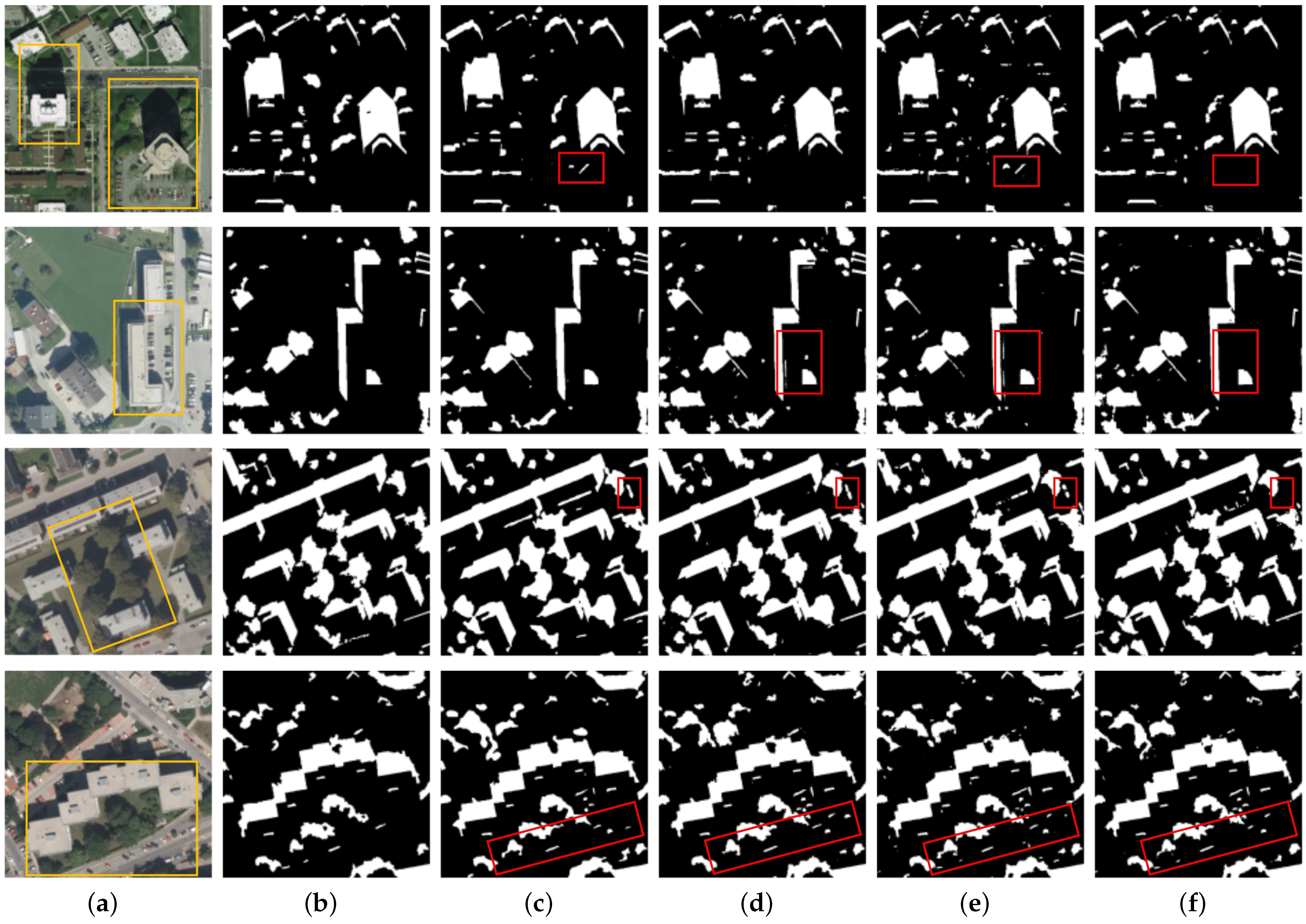
3.4. Qualitative Analysis

The qualitative comparison between MAMNet and the other four methods is shown in Figure 7. Images containing shadows of different sizes were selected for evaluation, demonstrating MAMNet’s ability to effectively detect objects of different sizes. It can be seen from the image in row 1 that MAMNet performed well in detecting large and irregular building shadows, while PSPNet and MSASDNet struggled, incorrectly identifying trees as shadows. In the image shown in row 2, our model could effectively detect relatively regular large building shadows, while ECANet and MSASDNet exhibited false detections. From the image presented in row 3, MAMNet demonstrates excellent detection of irregular tree shadows, closely matching the ground truth labels. Meanwhile, MAMNet can effectively distinguish between black objects and shaded areas without mistaking black cars for shadows, a common issue in the other three methods. In the image displayed in row 4, PSPNet and ECANet have missed detections, while MSASDNet exhibits false detections. In contrast, MAMNet can accurately detect small shadows without false detections and detect small tree shadows not labeled in the ground truth annotations as well. In summary, visualization of the experimental results shows that our model can effectively detect shadows of various scales while avoiding false detections in non-shadow areas.

4. Discussion

In this section, we will evaluate our model from the aspects of Advantages of the Proposed Method, Limitations, and Further Improvements.

4.1. Advantages of the Proposed Method

Shadow detection currently faces two main challenges. First, the differences in scale and morphological features of objects in the image lead to variations in shadow scale, affecting the network’s accuracy in detecting shadows at different scales. Second, some dark objects in the image, such as cars and roads, have spectral information and texture structures similar to shadows, making them prone to false positives. These factors collectively restrict the accuracy of shadow detection.

The method proposed in this paper demonstrates its superiority through comparative experimental results on the AISD dataset, significantly improving detection accuracy. Visualization results indicate that our model can effectively detect shadows of various sizes while successfully avoiding false positives in non-shadow areas, thereby addressing the two aforementioned issues. Most existing models rely heavily on spatial attention or multi-scale methods, often failing to fully utilize the deep features obtained during the decoding phase, which leads to a decrease in detection accuracy in multi-scale shadow scenarios. Additionally, these methods typically overlook important channel information. To address these limitations, we introduce a multi-scale spatial channel attention fusion module, which allows the model to fully leverage the deep features extracted by the encoder, accurately capturing the positions, shapes, and channel features of shadows in the images. As a result, this model exhibits greater flexibility when handling shadows of different sizes and effectively mitigates the impact of multi-scale shadow variations. Previous methods often resulted in erroneous detections in non-shadow areas due to insufficient utilization of pixel relationships. By introducing a criss-cross attention module, we can compare non-shadow pixels with other shadow and non-shadow pixels in the same row and column, allowing them to learn similar features. This approach significantly enhances the classification accuracy of non-shadow pixels and effectively prevents false detections in non-shadow areas. In the decoding phase, the continuous upsampling process can lead to the loss of important information, and relying solely on a single main branch weakens the effectiveness of the proposed MSCAF and CCA modules. To address this issue, we introduce an auxiliary branch module to assist the main branch in decision-making. This design enables the final output to integrate information from various stages, thereby maximizing the capabilities of both modules.

4.2. Limitations and Further Improvements

Although our method achieved the highest detection accuracy, there remains significant room for optimizing the model’s parameter count. The introduction of attention mechanisms and multi-branch structures has effectively enhanced the feature extraction capability, allowing the model to better capture complex information in images; however, it has also significantly increased the model’s parameter count and computational burden. Therefore, in future research, we will focus on reducing the model’s parameters while designing lightweight architectures to ensure that we maintain high accuracy while reducing resource consumption and memory usage.

Additionally, there are still issues with missing detection of small shadows in current shadow detection, which can impact the detection performance in practical applications. To address this challenge, we plan to develop specialized modules aimed at mitigating small shadow missed detection, employing innovative methods to enhance the model’s sensitivity to small shadows. This will allow our model to maintain excellent performance under various conditions, further improving its practicality and reliability.

5. Conclusions

We introduced a novel shadow detection model called MAMNet. MAMNet addressed the limitations of existing methods in detecting shadows of various scales, particularly small-sized shadows, which resulted in poor detection performance and the misidentification of dark, non-shaded areas as shadows. Through the multi-scale spatial channel attention fusion module, the model fully leveraged the deep features extracted by the encoder to capture the position, shape, and channel information of shadows at different scales. It adapted flexibly to shadow detection across varying scales and effectively mitigated the impact of multi-scale differences. By introducing the criss-cross attention module, non-shadow pixels were able to compare with other shadow and non-shadow pixels in the same rows and columns, learning similar features of the same type of pixels. This improved the classification accuracy of non-shadow pixels and reduced misclassification in non-shadow regions. Additionally, we developed an auxiliary branch module to assist the model in prediction. By integrating features from each stage of the decoding process, the final output can incorporate all information, fully leveraging the capabilities of the other two modules. We conducted experiments on the AISD dataset and compared our proposed method with 13 other state-of-the-art methods. Our model achieved the best performance across representative metrics, including overall accuracy (OA), precision, F1 score, and intersection over union (IOU). Additionally, visual analysis demonstrated that our model effectively detected shadows of various sizes while avoiding false detection in non-shadow areas. Our model presented a new viable approach for shadow detection in remote-sensing images.

References

1. Shimoni, M.; Tolt, G.; Perneel, C.; Ahlberg, J. Detection of Vehicles in Shadow Areas. In Proceedings of the 2011 3rd Workshop on Hyperspectral Image and Signal Processing: Evolution in Remote Sensing (WHISPERS), Lisbon, Portugal, 6–9 June 2011; pp. 1–4. [Google Scholar]
2. Chen, M.; Pang, S.K.; Cham, T.J.; Goh, A. Visual Tracking with Generative Template Model Based on Riemannian Manifold of Covariances. In Proceedings of the 14th International Conference on Information Fusion, Chicago, IL, USA, 5–8 July 2011; pp. 1–8. [Google Scholar]
3. Li, H.; Zhang, L.; Shen, H. An Adaptive Nonlocal Regularized Shadow Removal Method for Aerial Remote Sensing Images. IEEE Trans. Geosci. Remote Sens. 2014, 52, 106–120. [Google Scholar] [CrossRef]
4. Liu, J.; Fang, T.; Li, D. Shadow Detection in Remotely Sensed Images Based on Self-Adaptive Feature Selection. IEEE Trans. Geosci. Remote Sens. 2011, 49, 5092–5103. [Google Scholar]
5. Elbakary, M.I.; Iftekharuddin, K.M. Shadow Detection of Man-Made Buildings in High-Resolution Panchromatic Satellite Images. IEEE Trans. Geosci. Remote Sens. 2014, 52, 5374–5386. [Google Scholar] [CrossRef]
6. Silva, G.F.; Carneiro, G.B.; Doth, R.; Amaral, L.A.; Azevedo, D.F.G.D. Near Real-Time Shadow Detection and Removal in Aerial Motion Imagery Application. ISPRS J. Photogramm. Remote Sens. 2018, 140, 104–121. [Google Scholar] [CrossRef]
7. Li, D.; Wang, M.; Jiang, J. China’s High-Resolution Optical Remote Sensing Satellites and Their Mapping Applications. Geo-Spat. Inf. Sci. 2020, 24, 85–94. [Google Scholar] [CrossRef]
8. Li, D.; Wang, S.; Xiang, S.; Li, J.; Yang, Y.; Tang, X.-S. Dual-Stream Shadow Detection Network: Biologically Inspired Shadow Detection for Remote Sensing Images. Neural Comput. Appl. 2022, 34, 10039–10049. [Google Scholar] [CrossRef]
9. Wu, W.; Li, Q.; Zhang, Y.; Du, X.; Wang, H. Two-Step Urban Water Index (TSUWI): A New Technique for High-Resolution Mapping of Urban Surface Water. Remote Sens. 2018, 10, 1704. [Google Scholar] [CrossRef]
10. Xie, C.; Huang, X.; Zeng, W.; Fang, X. A Novel Water Index for Urban High-Resolution Eight-Band WorldView-2 Imagery. Int. J. Digit. Earth 2016, 10, 925–941. [Google Scholar] [CrossRef]
11. Mohajerani, S.; Saeedi, P. CPNet: A Context Preserver Convolutional Neural Network for Detecting Shadows in Single RGB Images. In Proceedings of the 2018 IEEE 20th International Workshop on Multimedia Signal Processing (MMSP), Vancouver, BC, Canada, 29–31 August 2018; pp. 1–5. [Google Scholar]
12. Luo, S.; Shen, H.; Li, H.; Chen, Y. Shadow Removal Based on Separated Illumination Correction for Urban Aerial Remote Sensing Images. Signal Process. 2019, 165, 197–208. [Google Scholar] [CrossRef]
13. Liasis, G.; Stavrou, S. Satellite Images Analysis for Shadow Detection and Building Height Estimation. ISPRS J. Photogramm. Remote Sens. 2016, 119, 437–450. [Google Scholar] [CrossRef]
14. Xie, Y.; Feng, D.; Xiong, S.; Zhu, J.; Liu, Y. Multi-Scene Building Height Estimation Method Based on Shadow in High Resolution Imagery. Remote Sens. 2021, 165, 2862. [Google Scholar] [CrossRef]
15. Xue, L.; Yang, S.; Li, Y.; Ma, J. An Automatic Shadow Detection Method for High-Resolution Remote Sensing Imagery Based on Polynomial Fitting. Int. J. Remote Sens. 2018, 40, 2986–3007. [Google Scholar] [CrossRef]
16. Kang, X.; Huang, Y.; Li, S.; Lin, H.; Benediktsson, J.A. Extended Random Walker for Shadow Detection in Very High Resolution Remote Sensing Images. IEEE Trans. Geosci. Remote Sens. 2018, 56, 867–876. [Google Scholar] [CrossRef]
17. Xie, Y.; Feng, D.; Chen, H.; Liao, Z.; Zhu, J.; Li, C.; Baik, S.W. An Omni-Scale Global-Local Aware Network for Shadow Extraction in Remote Sensing Imagery. ISPRS J. Photogramm. Remote Sens. 2022, 193, 29–44. [Google Scholar] [CrossRef]
18. Li, Y.; Gong, P.; Sasagawa, T. Integrated Shadow Removal Based on Photogrammetry and Image Analysis. Int. J. Remote Sens. 2007, 26, 3911–3929. [Google Scholar] [CrossRef]
19. Tolt, G.; Shimoni, M.; Ahlberg, J. A Shadow Detection Method for Remote Sensing Images Using VHR Hyperspectral and LIDAR Data. In Proceedings of the 2011 IEEE International Geoscience and Remote Sensing Symposium, Vancouver, BC, Canada, 24–29 July 2011; pp. 4423–4426. [Google Scholar]
20. Wang, Q.; Yan, L.; Yuan, Q.; Ma, Z. An Automatic Shadow Detection Method for VHR Remote Sensing Orthoimagery. Remote Sens. 2017, 9, 469. [Google Scholar] [CrossRef]
21. Mostafa, Y. A Review on Various Shadow Detection and Compensation Techniques in Remote Sensing Images. Can. J. Remote Sens. 2017, 43, 545–562. [Google Scholar] [CrossRef]
22. Li, Z.; Shen, H.; Li, H.; Xia, G.; Gamba, P.; Zhang, L. Multi-Feature Combined Cloud and Cloud Shadow Detection in GaoFen-1 Wide Field of View Imagery. Remote Sens. Environ. 2017, 191, 342–358. [Google Scholar] [CrossRef]
23. Ma, H.; Qin, Q.; Shen, X. Shadow Segmentation and Compensation in High Resolution Satellite Images. In Proceedings of the 2008 IEEE International Geoscience and Remote Sensing Symposium, Boston, MA, USA, 7–11 July 2008; pp. 1036–1039. [Google Scholar]
24. Song, H.; Huang, B.; Zhang, K. Shadow Detection and Reconstruction in High-Resolution Satellite Images Via Morphological Filtering and Example-Based Learning. Remote Sens. Environ. 2014, 52, 2545–2554. [Google Scholar] [CrossRef]
25. Lorenzi, L.; Melgani, F.; Mercier, G. A Complete Processing Chain for Shadow Detection and Reconstruction in VHR Images. IEEE Trans. Geosci. Remote Sens. 2012, 50, 3440–3452. [Google Scholar] [CrossRef]
26. Liu, H.; Liu, F.; Fan, X.; Huang, D. Polarized Self-Attention: Towards High-Quality Pixel-Wise Mapping. Neurocomputing 2022, 506, 158–167. [Google Scholar] [CrossRef]
27. Cao, Y.; Xu, J.; Lin, S.; Wei, F.; Hu, H. GCNet: Non-Local Networks Meet Squeeze-Excitation Networks and Beyond. In Proceedings of the 2019 IEEE/CVF International Conference on Computer Vision Workshop (ICCVW), Seoul, Republic of Korea, 27–28 October 2019; pp. 1971–1980. [Google Scholar]
28. Woo, S.; Park, J.; Lee, J.Y.; Kweon, I.S. CBAM: Convolutional Block Attention Module. In Proceedings of the European Conference on Computer Vision (ECCV), Munich, Germany, 8–14 September 2018; Springer International Publishing: Cham, Switzerland, 2018; pp. 3–19. [Google Scholar]
29. Long, J.; Shelhamer, E.; Darrell, T. Fully Convolutional Networks for Semantic Segmentation. In Proceedings of the 2015 IEEE Conference on Computer Vision and Pattern Recognition (CVPR), Boston, MA, USA, 7–12 June 2015; Springer International Publishing: Cham, Switzerland, 2018; pp. 3431–3440. [Google Scholar]
30. Ronneberger, O.; Fischer, P.; Brox, T. U-Net: Convolutional Networks for Biomedical Image Segmentation. In Proceedings of the Medical Image Computing and Computer-Assisted Intervention, Munich, Germany, 5–9 October 2015; Springer International Publishing: Cham, Switzerland, 2015; pp. 234–241. [Google Scholar]
31. Chen, L.-C.; Zhu, Y.; Papandreou, G.; Schroff, F.; Adam, H. Encoder–Decoder with Atrous Separable Convolution for Semantic Image Segmentation. In Proceedings of the European Conference on Computer Vision (ECCV), Munich, Germany, 8–14 September 2018; Springer International Publishing: Cham, Switzerland, 2018; pp. 801–818. [Google Scholar]
32. Zhao, H.; Shi, J.; Qi, X.; Wang, X.; Jia, J. Pyramid Scene Parsing Network. In Proceedings of the 2017 IEEE Conference on Computer Vision and Pattern Recognition (CVPR), Honolulu, HI, USA, 21–26 July 2017; pp. 6230–6239. [Google Scholar]
33. He, Z.; Zhang, Z.; Guo, M.; Wu, L.; Huang, Y. Adaptive Unsupervised Shadow-Detection Approach for Remote-Sensing Image Based on Multi Channel Features. Remote Sens. 2022, 14, 2756. [Google Scholar] [CrossRef]
34. Chen, Z.; Zhu, L.; Wan, L.; Wang, S.; Feng, W.; Heng, P. A Multi Task Mean Teacher for Semi-Supervised Shadow Detection. In Proceedings of the 2020 IEEE/CVF Conference on Computer Vision and Pattern Recognition (CVPR), Seattle, WA, USA, 13–19 June 2020; pp. 5610–5619. [Google Scholar]
35. Luo, S.; Li, H.; Shen, H. Deeply Supervised Convolutional Neural Network for Shadow Detection Based on a Novel Aerial Shadow Imagery Dataset. ISPRS J. Photogramm. Remote Sens. 2020, 167, 443–457. [Google Scholar] [CrossRef]
36. Jin, Y.; Xu, W.; Hu, Z.; Jia, H.; Luo, X.; Shao, D. GSCA-UNet: Towards Automatic Shadow Detection in Urban Aerial Imagery with Global-Spatial-Context Attention Module. Remote Sens. 2020, 12, 2864. [Google Scholar] [CrossRef]
37. Luo, S.; Li, H.; Zhu, R.; Gong, Y.; Shen, H. ESPFNet: An Edge-Aware Spatial Pyramid Fusion Network for Salient Shadow Detection in Aerial Remote Sensing Images. IEEE J. Sel. Top. Appl. Earth Obs. Remote Sens. 2021, 14, 4633–4646. [Google Scholar] [CrossRef]
38. Zhu, Q.; Yang, Y.; Sun, X.; Guo, M. CDANet: Contextual Detail-Aware Network for High-Spatial-Resolution Remote-Sensing Imagery Shadow Detection. IEEE Trans. Geosci. Remote Sens. 2022, 60, 5617415. [Google Scholar] [CrossRef]
39. Liu, D.; Zhang, J.; Wu, Y.; Zhang, Y. A Shadow Detection Algorithm Based on Multiscale Spatial Attention Mechanism for Aerial Remote Sensing Images. IEEE Geosci. Remote Sens. Lett. 2022, 19, 6003905. [Google Scholar] [CrossRef]
40. Zhang, S.; Cao, Y.; Sui, B. DTHNet: Dual-Stream Network Based on Transformer and High-Resolution Representation for Shadow Extraction from Remote Sensing Imagery. IEEE Geosci. Remote Sens. Lett. 2023, 20, 8000905. [Google Scholar] [CrossRef]
41. Zhang, J.; Shi, X.; Zheng, C.; Wu, J.; Li, Y. MRPFA-Net for Shadow Detection in Remote-Sensing Images. IEEE Trans. Geosci. Remote Sens. 2023, 61, 5514011. [Google Scholar] [CrossRef]
42. Chen, H.; Feng, D.; Cao, S.; Xu, W.; Xie, Y.; Zhu, J.; Zhang, H. Slice-to-Slice Context Transfer and Uncertain Region Calibration Network for Shadow Detection in Remote Sensing Imagery. ISPRS J. Photogramm. Remote Sens. 2023, 203, 166–182. [Google Scholar] [CrossRef]
43. Huang, Z.; Wang, X.; Wei, Y.; Huang, L.; Shi, H.; Liu, W.; Huang, T.S. CCNet: Criss-Cross Attention for Semantic Segmentation. IEEE Trans. Pattern Anal. Mach. Intell. 2023, 45, 6896–6908. [Google Scholar] [CrossRef]
Figure 1. Existing challenges in remote-sensing image shadow detection.
Remotesensing 16 04789 g001
Figure 2. The entire flow of shadow detection.
Remotesensing 16 04789 g002
Figure 3. Illustration of the proposed MAMNet.
Remotesensing 16 04789 g003
Figure 4. Illustration of the proposed multi-scale spatial channel attention fusion module.
Remotesensing 16 04789 g004
Figure 5. Structure of the auxiliary branch.
Remotesensing 16 04789 g005
Figure 6. AISD dataset pictures and their labels.
Remotesensing 16 04789 g006
Figure 7. Comparison of the shadow detection results in the AISD dataset. (a) Input image. (b) Ground truth. (c) PSPNet. (d) ECANet. (e) MSASDNet. (f) MAMNet (ours).
Remotesensing 16 04789 g007