
A High-Resolution Spotlight Imaging Algorithm via Modified Second-Order Space-Variant Wavefront Curvature Correction for MEO/HM-BiSAR
 , ,
, ,
Abstract
1. Introduction
2. The Geometry and Range Models
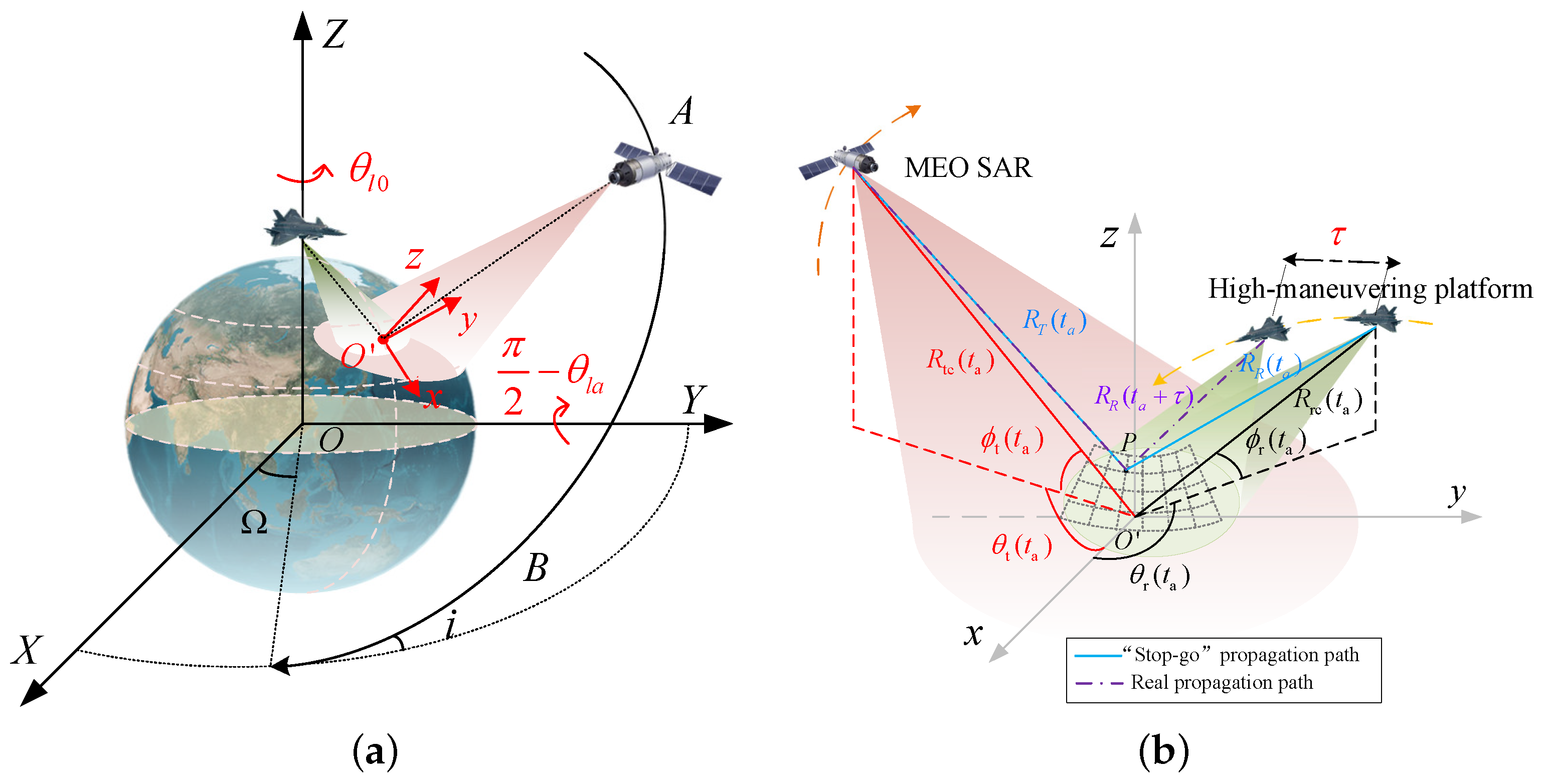
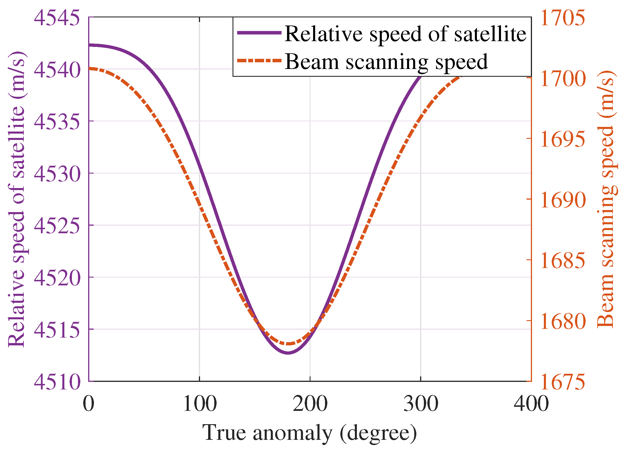
2.1. MEO SAR Characteristic Analysis and Coordinate System Transformation
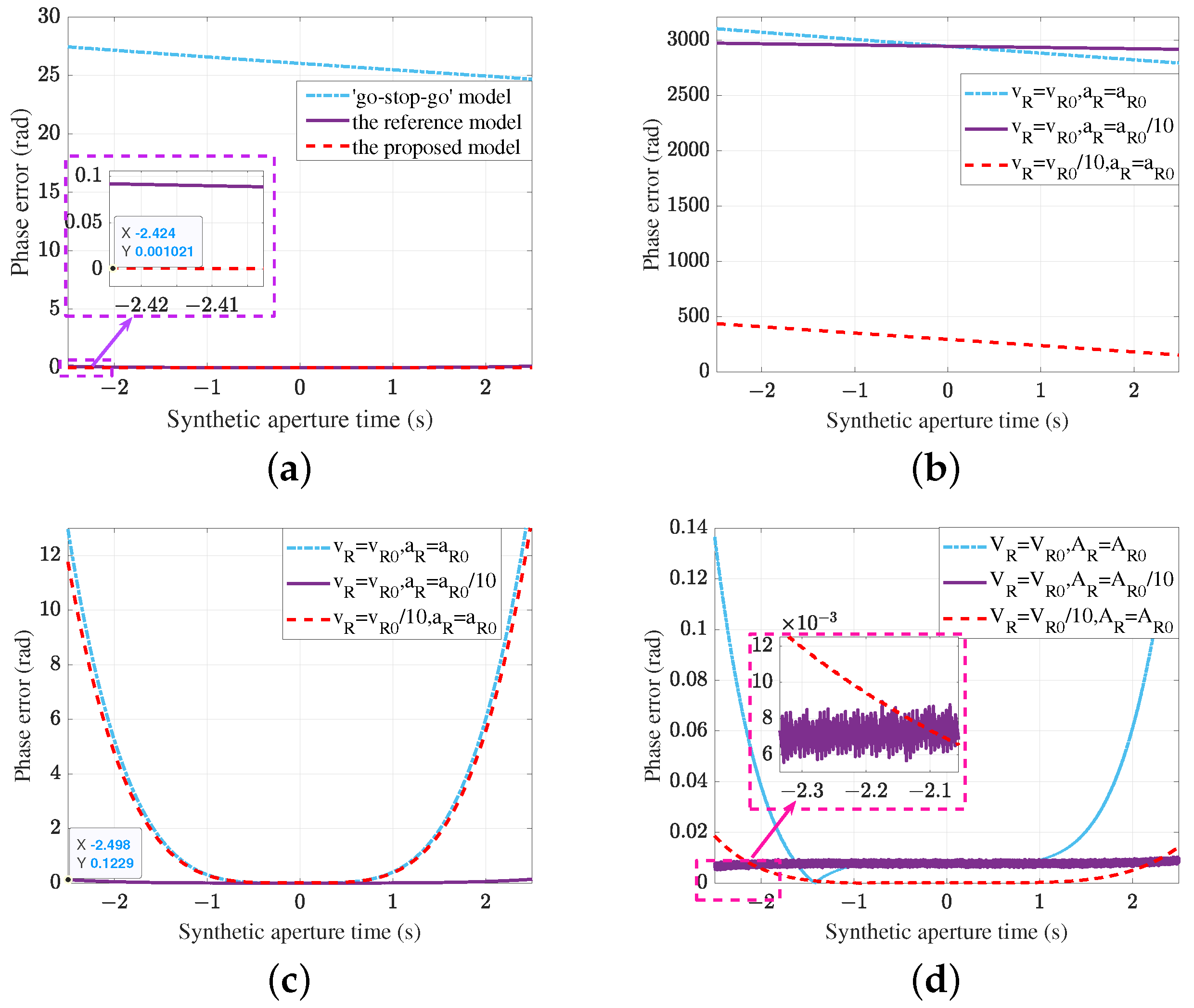
2.2. Motion Range Model and Echo Model
3. The Polar Formatting Process for BiSAR
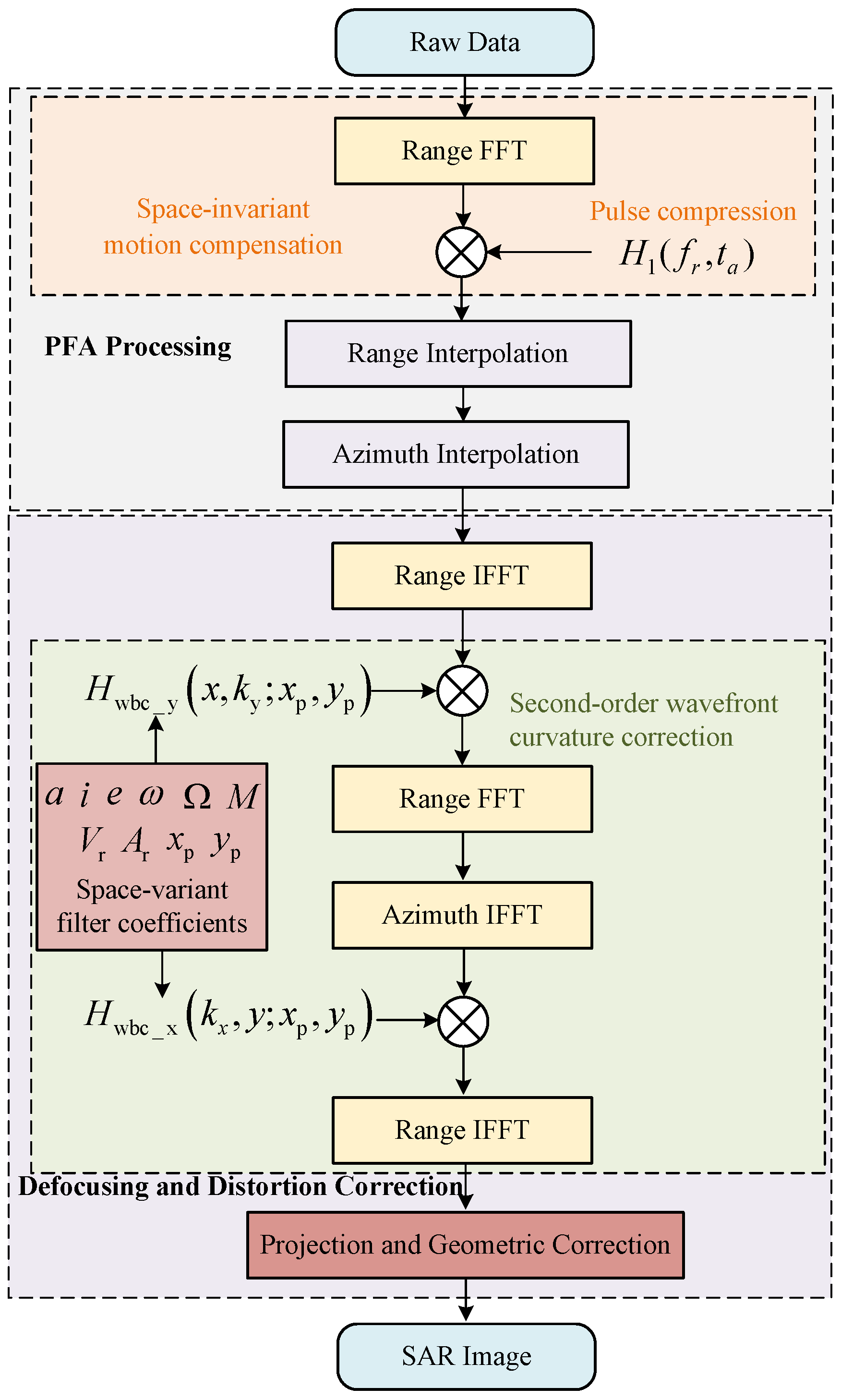
4. The MSSWCC Imaging Algorithm for MEO/HM-BiSAR
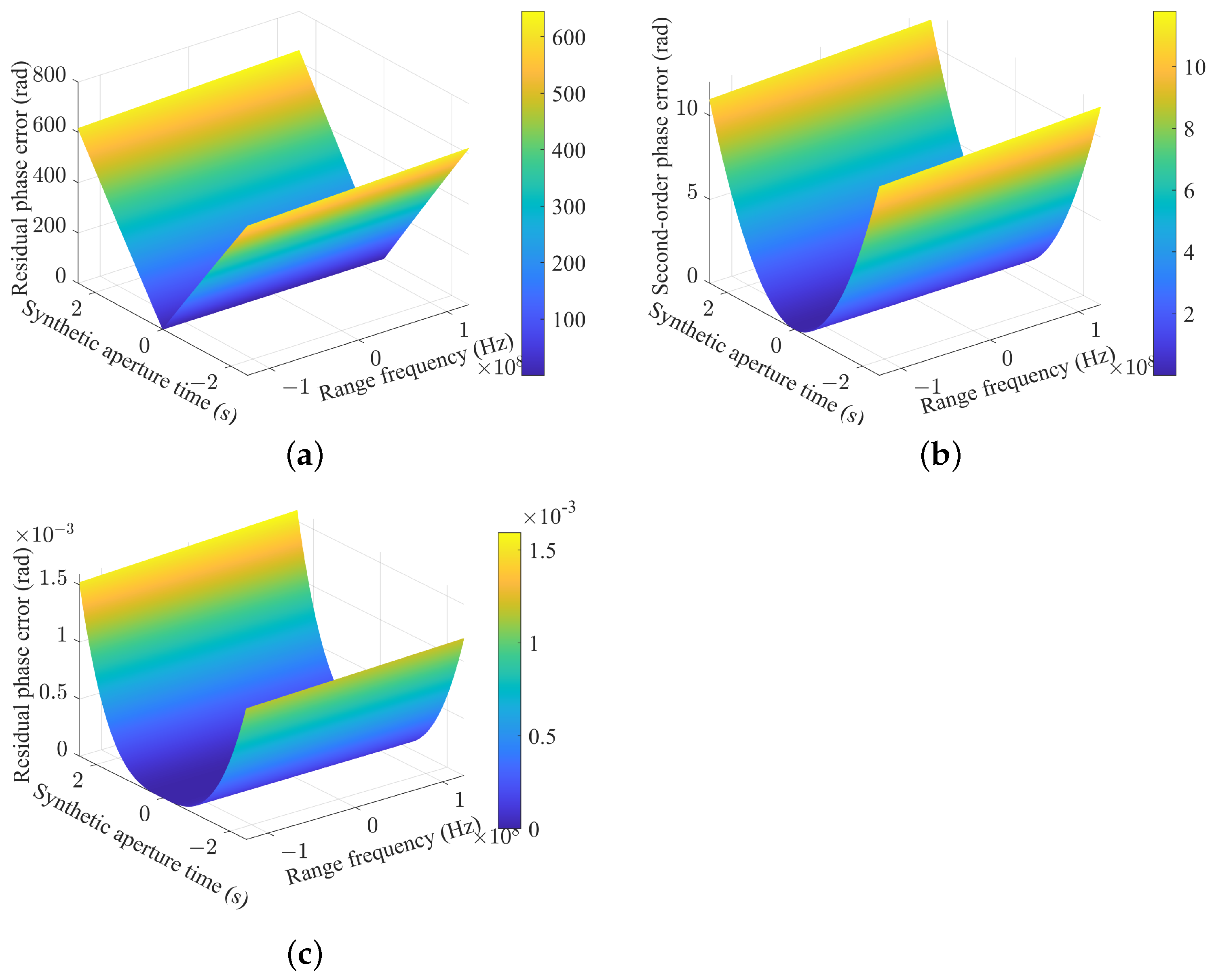
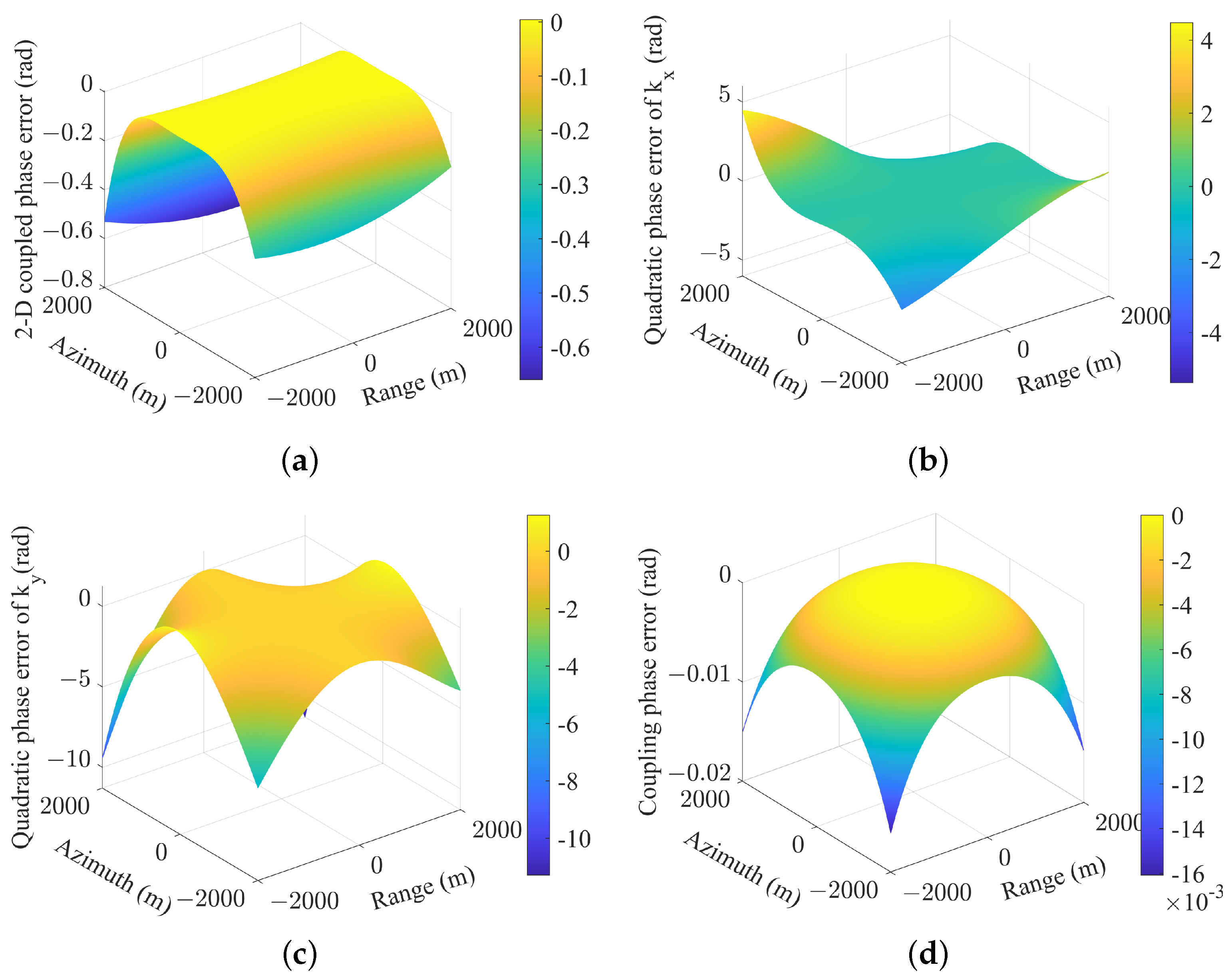
4.1. The Compensation of Wavefront Curvature Error
4.2. Geometric Correction and Projection
| Algorithm 1 Geometric Distortion Correction Method |
|
4.3. Computation Cost
5. Experiment Results
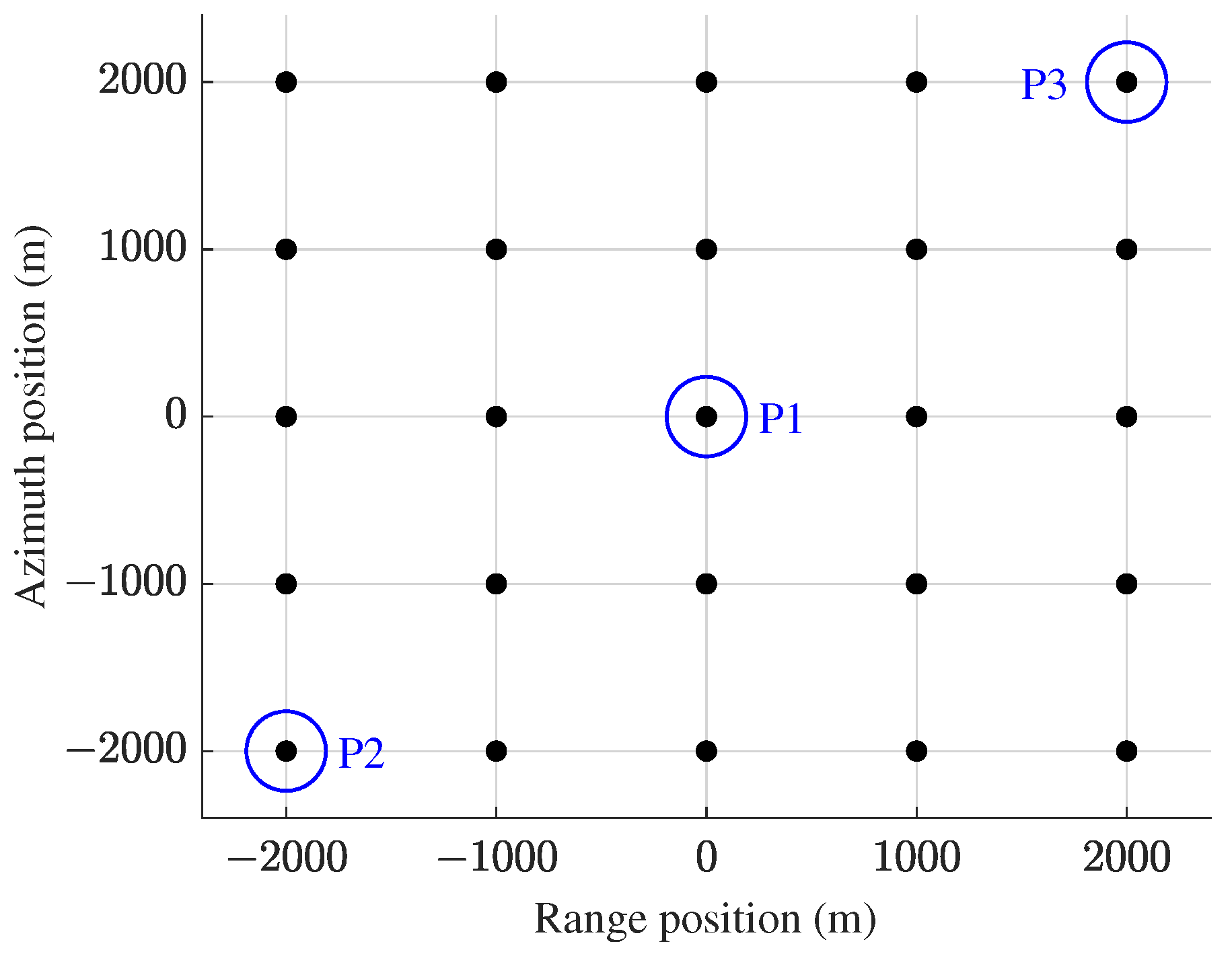
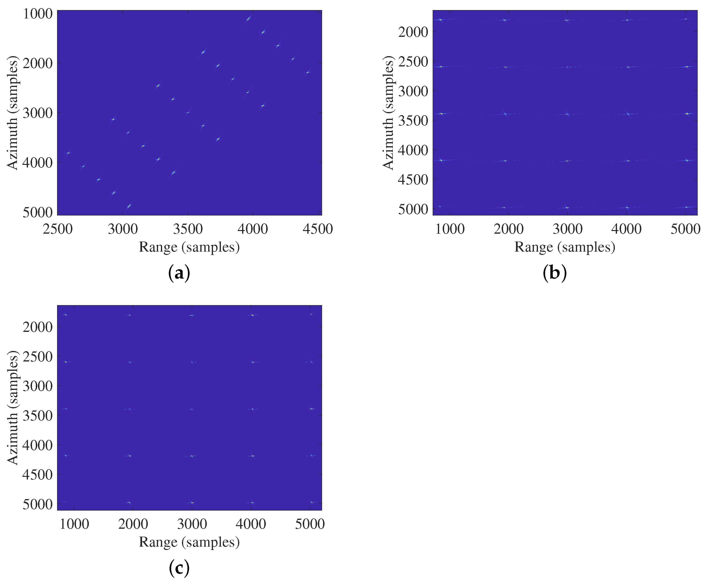
5.1. Simulation of Point Targets
5.2. Real BiSAR Experiment
6. Discussion
7. Conclusions
Author Contributions
Funding
Data Availability Statement
Conflicts of Interest
Appendix A
Appendix B
Appendix C
References
- Matar, J.; Lopez-Dekker, P.; Krieger, G. Potentials and Limitations of MEO SAR. In Proceedings of the European Conference on Synthetic Aperture Radar, Hamburg, Germany, 6–9 June 2016; pp. 1–5. [Google Scholar]
- Matar, J.; Rodriguez-Cassola, M.; Krieger, G.; López-Dekker, P.; Moreira, A. MEO SAR: System Concepts and Analysis. IEEE Trans. Geosci. Remote Sens. 2020, 58, 1313–1324. [Google Scholar] [CrossRef]
- Liu, W.; Sun, G.C.; Xia, X.G.; You, D.; Xing, M.; Bao, Z. Highly Squinted MEO SAR Focusing Based on Extended Omega-K Algorithm and Modified Joint Time and Doppler Resampling. IEEE Trans. Geosci. Remote Sens. 2019, 57, 9188–9200. [Google Scholar] [CrossRef]
- Chen, J.; Xing, M.; Sun, G.C.; Gao, Y.; Liu, W.; Guo, L.; Lan, Y. Focusing of Medium-Earth-Orbit SAR Using an ASE-Velocity Model Based on MOCO Principle. IEEE Trans. Geosci. Remote Sens. 2018, 56, 3963–3975. [Google Scholar] [CrossRef]
- Liu, W.; Sun, G.C.; Xing, M.; Li, H.; Bao, Z. Focusing of MEO SAR Data Based on Principle of Optimal Imaging Coordinate System. IEEE Trans. Geosci. Remote Sens. 2020, 58, 5477–5489. [Google Scholar] [CrossRef]
- Matar, J.; Rodriguez-Cassola, M.; Krieger, G.; Moreira, A. On the Equivalence of LEO-SAR Constellations and Complex High-Orbit SAR Systems for the Monitoring of Large-Scale Processes. IEEE Geosci. Remote Sens. Lett. 2024, 21, 8500205. [Google Scholar] [CrossRef]
- Zhang, Y.; Ren, H.; Lu, Z.; Yang, X.; Li, G. Focusing of Highly Squinted Bistatic SAR With MEO Transmitter and High Maneuvering Platform Receiver in Curved Trajectory. IEEE Trans. Geosci. Remote Sens. 2024, 62, 5227522. [Google Scholar] [CrossRef]
- Song, X.; Li, Y.; Wu, C.; Sun, Z.; Cen, X.; Zhang, T. A New Frenquency-Domain Imaging for High-maneuverability Bistatic Forward-looking SAR. In Proceedings of the 2021 CIE International Conference on Radar (Radar), Haikou, China, 15–19 December 2021; pp. 778–782. [Google Scholar] [CrossRef]
- Hu, X.; Xie, H.; Yi, S.; Zhang, L.; Lu, Z. An Improved NLCS Algorithm Based on Series Reversion and Elliptical Model Using Geosynchronous Spaceborne—Airborne UHF UWB Bistatic SAR for Oceanic Scene Imaging. Remote Sens. 2024, 16, 1131. [Google Scholar]
- Wang, Z.; Liu, F.; Zeng, T.; Wang, C. A Novel Motion Compensation Algorithm Based on Motion Sensitivity Analysis for Mini-UAV-Based BiSAR System. IEEE Trans. Geosci. Remote Sens. 2022, 60, 5205813. [Google Scholar] [CrossRef]
- Zhang, S.; Liu, F.; Wang, Z.; Wang, C.; Lv, R.; Yao, D. A LEO Spaceborne-Airborne Bistatic SAR Imaging Experiment. In Proceedings of the IEEE International Conference on Signal Processing, Communications and Computing, ICSPCC, Bali, Indonesia, 19–22 August 2022; pp. 1–5. [Google Scholar] [CrossRef]
- Tang, S.; Guo, P.; Zhang, L.; Lin, C. Modeling and precise processing for spaceborne transmitter/missile-borne receiver SAR signals. Remote Sens. 2019, 11, 346. [Google Scholar]
- Sun, Z.; Wu, J.; Li, Z.; An, H.; He, X. Geosynchronous Spaceborne–Airborne Bistatic SAR Data Focusing Using a Novel Range Model Based on One-Stationary Equivalence. IEEE Trans. Geosci. Remote Sens. 2021, 59, 1214–1230. [Google Scholar] [CrossRef]
- Zhang, Y.; Xiong, W.; Dong, X.; Hu, C. A Novel Azimuth Spectrum Reconstruction and Imaging Method for Moving Targets in Geosynchronous Spaceborne–Airborne Bistatic Multichannel SAR. IEEE Trans. Geosci. Remote Sens. 2020, 58, 5976–5991. [Google Scholar] [CrossRef]
- An, H.; Wu, J.; Teh, K.C.; Sun, Z.; Yang, J. Geosynchronous Spaceborne–Airborne Bistatic SAR Imaging Based on Fast Low-Rank and Sparse Matrices Recovery. IEEE Trans. Geosci. Remote Sens. 2022, 60, 5207714. [Google Scholar] [CrossRef]
- Tang, W.; Huang, B.; Wang, W.Q.; Zhang, S.; Liu, W.; Wang, Y. A Novel Imaging Algorithm for Forward-looking GEO/Missile-borne Bistatic SAR. In Proceedings of the Asia-Pacific Conference on Synthetic Aperture Radar APSAR, Xiamen, China, 26–29 November 2019; pp. 1–4. [Google Scholar] [CrossRef]
- Zhang, S.; Gao, Y.; Xing, M.; Guo, R.; Chen, J.; Liu, Y. Ground Moving Target Indication for the Geosynchronous-Low Earth Orbit Bistatic Multichannel SAR System. IEEE J. Sel. Topics Appl. Earth Observ. Remote Sens. 2021, 14, 5072–5090. [Google Scholar] [CrossRef]
- Wu, J.; Sun, Z.; An, H.; Qu, J.; Yang, J. Azimuth Signal Multichannel Reconstruction and Channel Configuration Design for Geosynchronous Spaceborne–Airborne Bistatic SAR. IEEE Trans. Geosci. Remote Sens. 2019, 57, 1861–1872. [Google Scholar] [CrossRef]
- Ding, J.; Li, Y.; Li, M.; Wang, J. Focusing High Maneuvering Bistatic Forward-Looking SAR With Stationary Transmitter Using Extended Keystone Transform and Modified Frequency Nonlinear Chirp Scaling. IEEE J. Sel. Top. Appl. Earth Obs. Remote Sens. 2022, 15, 2476–2492. [Google Scholar] [CrossRef]
- Song, X.; Li, Y.; Zhang, T.; Li, L.; Gu, T. Focusing High-Maneuverability Bistatic Forward-Looking SAR Using Extended Azimuth Nonlinear Chirp Scaling Algorithm. IEEE Trans. Geosci. Remote Sens. 2022, 60, 5240814. [Google Scholar] [CrossRef]
- Miao, Y.; Wu, J.; Li, Z.; Yang, J. A Generalized Wavefront-Curvature-Corrected Polar Format Algorithm to Focus Bistatic SAR Under Complicated Flight Paths. IEEE J. Sel. Topics Appl. Earth Observ. Remote Sens. 2020, 13, 3757–3771. [Google Scholar] [CrossRef]
- Xie, H.; Hu, J.; Duan, K.; Wang, G. High-Efficiency and High-Precision Reconstruction Strategy for P-Band Ultra-Wideband Bistatic Synthetic Aperture Radar Raw Data Including Motion Errors. IEEE Access 2020, 8, 31143–31158. [Google Scholar] [CrossRef]
- Wang, Y.; Liu, Y.; Li, Z.; Suo, Z.; Fang, C.; Chen, J. High-Resolution Wide-Swath Imaging of Spaceborne Multichannel Bistatic SAR with Inclined Geosynchronous Illuminator. IEEE Geosci. Remote Sens. Lett. 2017, 14, 2380–2384. [Google Scholar]
- Pu, W.; Wu, J.; Huang, Y.; Yang, J.; Yang, H. Fast Factorized Backprojection Imaging Algorithm Integrated With Motion Trajectory Estimation for Bistatic Forward-Looking SAR. IEEE J. Sel. Top. Appl. Earth Obs. Remote Sens. 2019, 12, 3949–3965. [Google Scholar]
- Zhou, S.; Yang, L.; Zhao, L.; Wang, Y.; Xing, M. A New Fast Factorized Back Projection Algorithm for Bistatic Forward-Looking SAR Imaging Based on Orthogonal Elliptical Polar Coordinate. IEEE J. Sel. Top. Appl. Earth Obs. Remote Sens. 2019, 12, 1508–1520. [Google Scholar]
- Hu, X.; Xie, H.; Zhang, L.; Hu, J.; He, J.; Yi, S.; Jiang, H.; Xie, K. Fast Factorized Backprojection Algorithm in Orthogonal Elliptical Coordinate System for Ocean Scenes Imaging Using Geosynchronous Spaceborne—Airborne VHF UWB Bistatic SAR. Remote Sens. 2023, 15, 2215. [Google Scholar]
- Yuan, Y.; Chen, S.; Zhao, H. An Improved RD Algorithm for Maneuvering Bistatic Forward-Looking SAR Imaging with a Fixed Transmitter. Sensors 2017, 17, 1152. [Google Scholar]
- Li, C.; Zhang, H.; Deng, Y.; Wang, R.; Liu, K.; Liu, D.; Jin, G.; Zhang, Y. Focusing the L-Band Spaceborne Bistatic SAR Mission Data Using a Modified RD Algorithm. IEEE Trans. Geosci. Remote Sens. 2020, 58, 294–306. [Google Scholar] [CrossRef]
- Wong, F.H.; Cumming, I.G.; Neo, Y.L. Focusing Bistatic SAR Data Using the Nonlinear Chirp Scaling Algorithm. IEEE Trans. Geosci. Remote Sens. 2008, 46, 2493–2505. [Google Scholar] [CrossRef]
- Chen, S.; Yuan, Y.; Zhang, S.; Zhao, H.; Chen, Y. A New Imaging Algorithm for Forward-Looking Missile-Borne Bistatic SAR. IEEE J. Sel. Top. Appl. Earth Obs. Remote Sens. 2016, 9, 1543–1552. [Google Scholar] [CrossRef]
- Deng, Y. Focus Improvement of Airborne High-Squint Bistatic SAR Data Using Modified Azimuth NLCS Algorithm Based on Lagrange Inversion Theorem. Remote Sens. 2021, 13, 1916. [Google Scholar]
- Wang, Z.; Guo, Q.; Tian, X.; Chang, T.; Cui, H.L. Millimeter-Wave Image Reconstruction Algorithm for One-Stationary Bistatic SAR. IEEE Trans. Microw. Theory Tech. 2020, 68, 1185–1194. [Google Scholar] [CrossRef]
- Wang, X.; Zhu, D.; Mao, X.; Zhu, Z. Space-Variant Filtering for Wavefront Curvature Correction in Polar Formatted Bistatic SAR Image. IEEE Trans. Aerosp. Electron. Syst. 2012, 48, 940–950. [Google Scholar] [CrossRef]
- Zhang, Q.; Wu, J.; Li, Z.; Miao, Y.; Huang, Y.; Yang, J. PFA for Bistatic Forward-Looking SAR Mounted on High-Speed Maneuvering Platforms. IEEE Trans. Geosci. Remote Sens. 2019, 57, 6018–6036. [Google Scholar] [CrossRef]
- Wang, F.; Zhang, L.; Cao, Y.; Yeo, T.S.; Lu, J.; Han, J.; Peng, Z. High-Resolution Bistatic Spotlight SAR Imagery With General Configuration and Accelerated Track. IEEE Trans. Geosci. Remote Sens. 2023, 61, 5213218. [Google Scholar] [CrossRef]
- Han, S.; Zhu, D.; Mao, X. A Modified Space-Variant Phase Filtering Algorithm of PFA for Bistatic SAR. IEEE Geosci. Remote Sens. Lett. 2022, 19, 4008005. [Google Scholar] [CrossRef]
- Shi, T.; Mao, X.; Jakobsson, A.; Liu, Y. Efficient BiSAR PFA Wavefront Curvature Compensation for Arbitrary Radar Flight Trajectories. IEEE Trans. Geosci. Remote Sens. 2023, 61, 5221514. [Google Scholar] [CrossRef]
- Huang, L.; Qiu, X.; Hu, D.; Ding, C. An advanced 2-D spectrum for high-resolution and MEO spaceborne SAR. In Proceedings of the 2009 2nd Asian-Pacific Conference on Synthetic Aperture Radar, Xi’an, China, 26–30 October 2009. [Google Scholar]
- Qian, G.; Wang, Y. Analysis of Modeling and 2-D Resolution of Satellite–Missile Borne Bistatic Forward-Looking SAR. IEEE Trans. Geosci. Remote Sens. 2023, 61, 5222314. [Google Scholar] [CrossRef]
- Huo, T.; Li, Y.; Yang, C.; Cao, C.; Wang, Y. A Novel Imaging Method for MEO SAR-GMTI Systems. In Proceedings of the IGARSS 2022-2022 IEEE International Geoscience and Remote Sensing Symposium, Kuala Lumpur, Malaysia, 17–22 July 2022; pp. 2498–2501. [Google Scholar] [CrossRef]
- Tang, S.; Zhang, L.; Guo, P.; Liu, G.; Sun, G.C. Acceleration Model Analyses and Imaging Algorithm for Highly Squinted Airborne Spotlight-Mode SAR with Maneuvers. IEEE J. Sel. Top. Appl. Earth Obs. Remote Sens. 2015, 8, 1120–1131. [Google Scholar] [CrossRef]
- Zheng, Z.; Tan, G.; Jiang, D. A Bidirectional Resampling Imaging Algorithm for High Maneuvering Bistatic Forward-Looking SAR Based on Chebyshev Orthogonal Decomposition. IEEE Trans. Geosci. Remote Sens. 2024, 62, 5211512. [Google Scholar] [CrossRef]
- An, H.; Wu, J.; Teh, K.C.; Sun, Z.; Yang, J. Nonambiguous Image Formation for Low-Earth-Orbit SAR with Geosynchronous Illumination Based on Multireceiving and CAMP. IEEE Trans. Geosci. Remote Sens. 2021, 59, 348–362. [Google Scholar] [CrossRef]
- Deng, H.; Li, Y.; Liu, M.; Mei, H.; Quan, Y. A Space-Variant Phase Filtering Imaging Algorithm for Missile-Borne BiSAR With Arbitrary Configuration and Curved Track. IEEE Sens. J. 2018, 18, 3311–3326. [Google Scholar] [CrossRef]
- Guo, Y.; Yu, Z.; Li, J.; Li, C. Focusing Spotlight-Mode Bistatic GEO SAR with a Stationary Receiver Using Time-Doppler Resampling. IEEE Sens. J. 2020, 20, 10766–10778. [Google Scholar] [CrossRef]
- An, H.; Wu, J.; He, Z.; Li, Z.; Yang, J. Geosynchronous Spaceborne–Airborne Multichannel Bistatic SAR Imaging Using Weighted Fast Factorized Backprojection Method. IEEE Geosci. Remote Sens. Lett. 2019, 16, 1590–1594. [Google Scholar] [CrossRef]
- Gorham, L.; Rigling, B. Fast corrections for polar format algorithm with a curved flight path. IEEE Trans. Aerosp. Electron. Syst. 2016, 52, 2815–2824. [Google Scholar] [CrossRef]
- Xiong, T.; Li, Y.; Li, Q.; Wu, K.; Zhang, L.; Zhang, Y.; Mao, S.; Han, L. Using an Equivalence-Based Approach to Derive 2-D Spectrum of BiSAR Data and Implementation Into an RDA Processor. IEEE Trans. Geosci. Remote Sens. 2021, 59, 4765–4774. [Google Scholar] [CrossRef]
- Xin, N. Research on Key Technique of Highly Squinted Sliding SpotlightSAR Imaging with Varied Receiving Range Bin. J. Electron. Inf. Technol. 2016, 38, 3122–3128. [Google Scholar]
- Xin, N.; Shijian, S.; Hui, Y.; Ying, L.; Long, Z.; Wanming, L. A wide-field SAR polar format algorithm based on quadtree sub-image segmentation. In Proceedings of the IGARSS 2018-2018 IEEE International Geoscience and Remote Sensing Symposium, Valencia, Spain, 22–27 July 2018; pp. 9355–9358. [Google Scholar] [CrossRef]
- Nie, X.; Zhuang, L.; Shen, S. A Quadtree Beam-Segmenting Based Wide-Swath SAR Polar Format Algorithm. IEEE Access 2020, 8, 147682–147691. [Google Scholar] [CrossRef]


| Orbital Elements | Values |
|---|---|
| Semimajor axis (km) | 16,371 |
| Inclination (deg) | 60 |
| Eccentricity | 0.003 |
| Argument of perigee (deg) | 90 |
| Ascending node (deg) | 105 |
| True anomaly (deg) | 0–360 |
| Antenna look-down angle (deg) | 10 |
| Beam direction angle (deg) | 90 |
| Orbital Elements | Values |
|---|---|
| Receiver position (km) | (−10, −40, 60) |
| Receiver velocity (m/s) | (20, 920, −500) |
| Receiver acceleration (m/s2) | (0, 50, −50) |
| Carrier frequency (GHz) | 5.4 |
| Bandwidth (MHz) | 200 |
| Sampling frequency (MHz) | 250 |
| PRF (Hz) | 3000 |
| Pulse duration (us) | 2 |
| Algorithm | Coordinate of P1 | Coordinate of P2 | Coordinate of P3 |
|---|---|---|---|
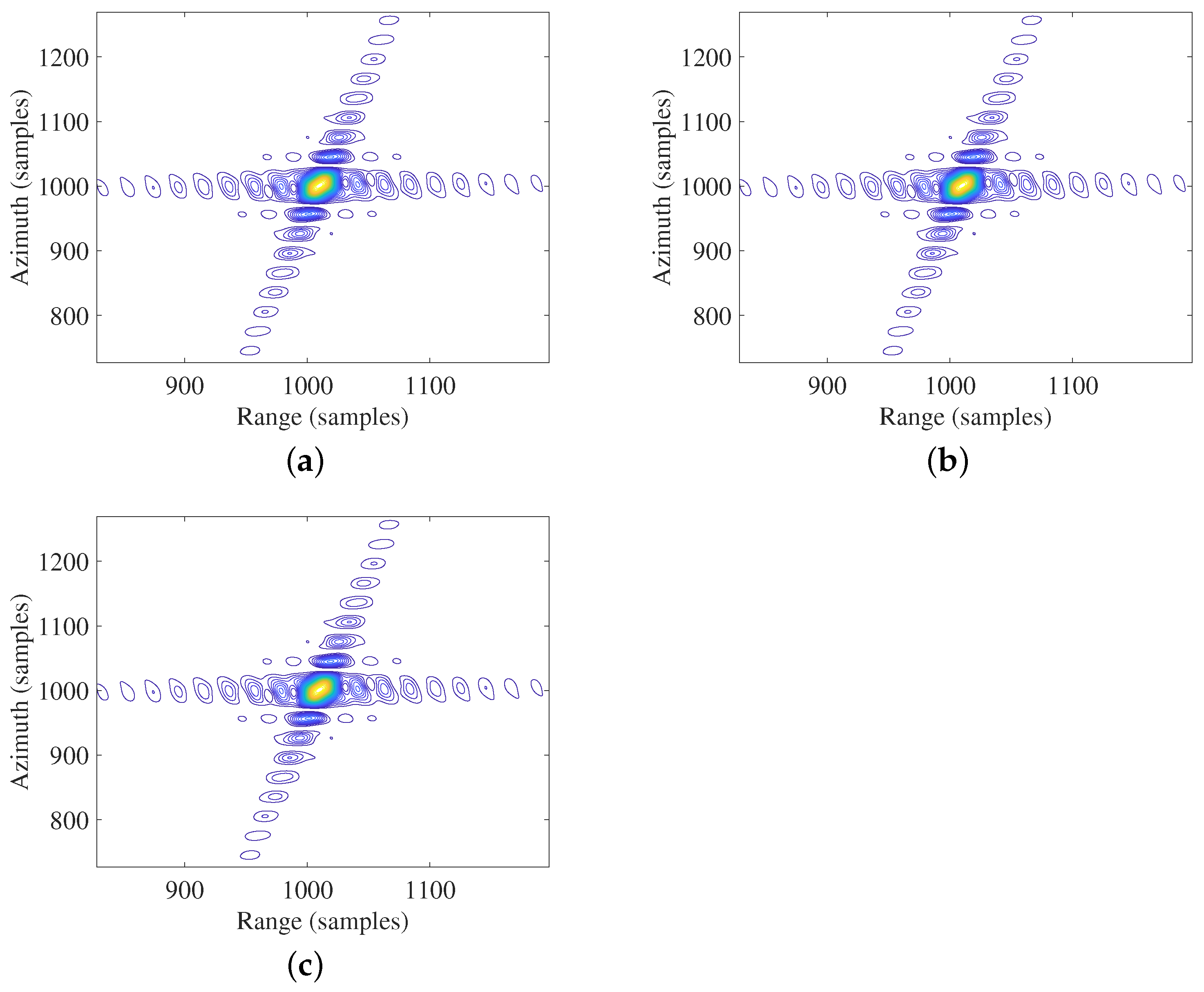
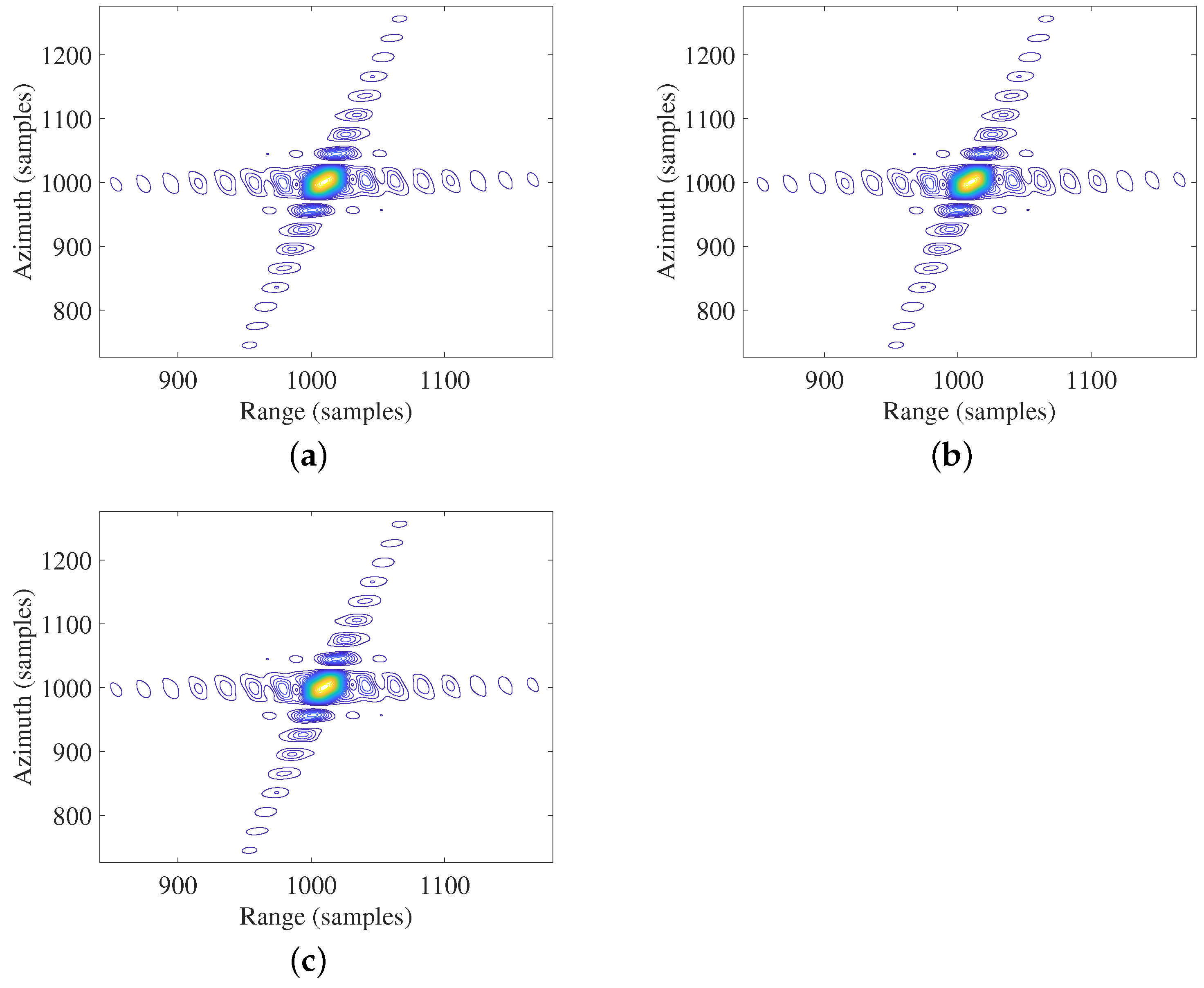
| The sub-image PFA algorithm | (0 m, 0 m) | (−1870 m, −2023 m) | (2135 m, 1974 m) |
| The proposed algorithm | (0 m, 0 m) | (−2000 m, −2000 m) | (2000 m, 2000 m) |
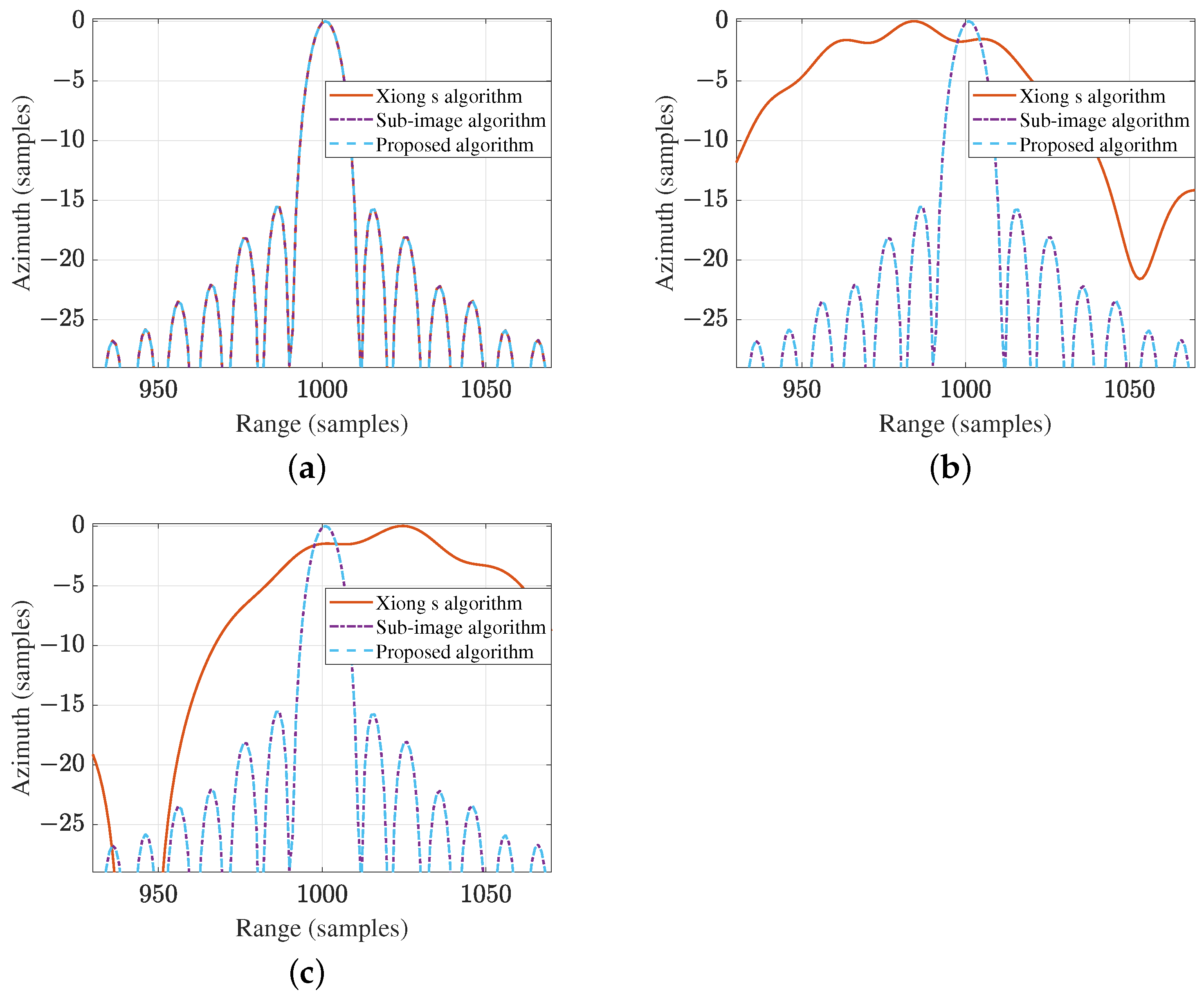
| Algorithm | Point | PSLR/dB | ISLR/dB | Res-A/m | Res-R/m |
|---|---|---|---|---|---|
| Xiong’s algorithm | P1 | −15.56 | −12.86 | 1.599 | 0.840 |
| P2 | −1.702 | −5.592 | 12.85 | 0.840 | |
| P3 | −1.492 | −6.506 | 15.35 | 0.840 | |
| Proposed algorithm | P1 | −15.67 | −12.89 | 1.599 | 0.840 |
| P2 | −15.59 | −12.92 | 1.599 | 0.840 | |
| P3 | −15.42 | −12.88 | 1.600 | 0.840 | |
| BP algorithm | P1 | −15.70 | −12.89 | 1.600 | 0.840 |
| P2 | −15.70 | −12.89 | 1.600 | 0.840 | |
| P3 | −15.70 | −12.89 | 1.600 | 0.840 |
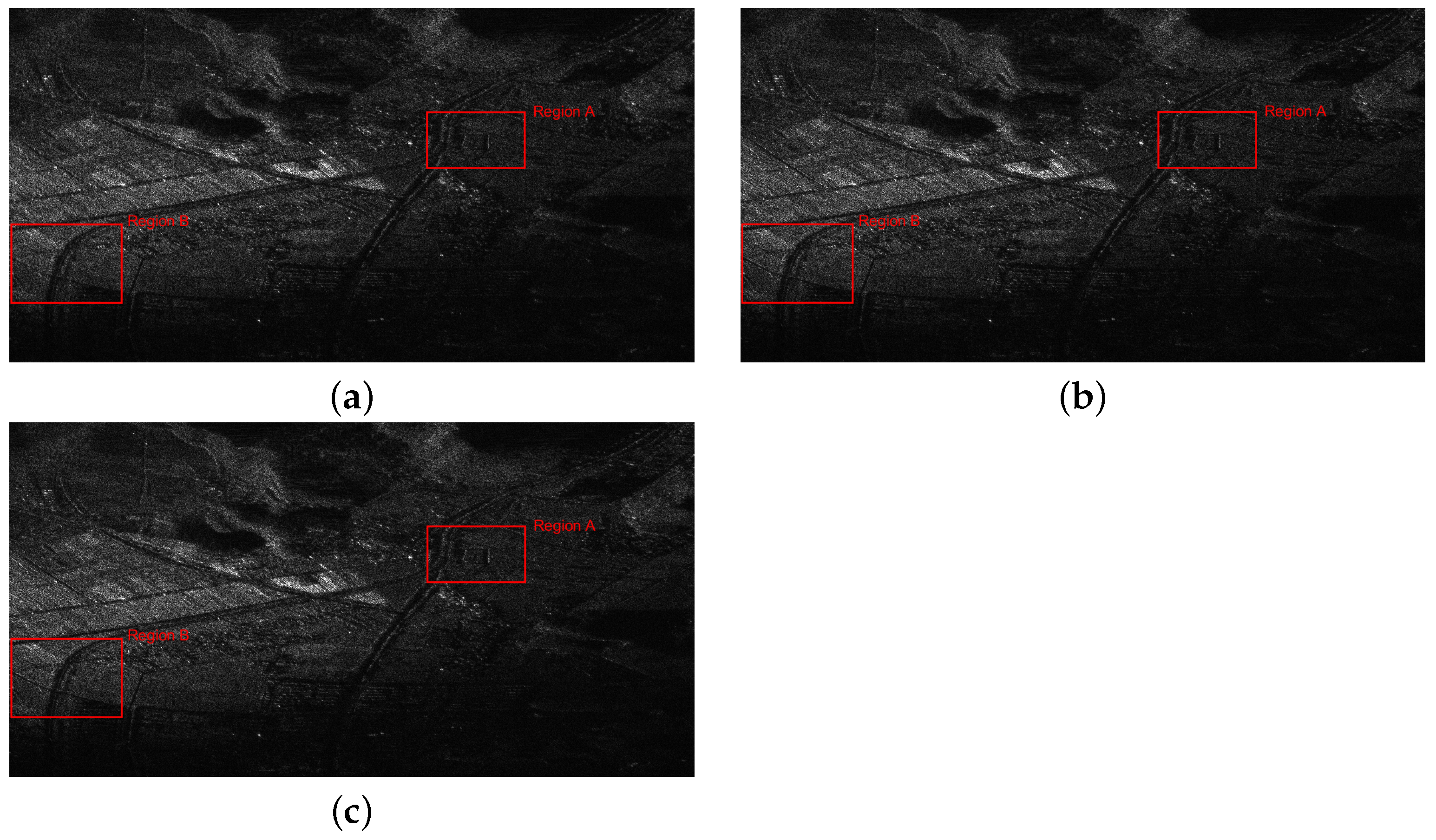
| Algorithm | Region A | Region B | ||
|---|---|---|---|---|
| Image Entropy | Image Contrast | Image Entropy | Image Contrast | |
| Without MSSWCC | 5.955 | 0.656 | 6.683 | 0.722 |
| Proposed algorithm | 5.927 | 0.659 | 6.350 | 0.750 |
| BP algorithm | 5.927 | 0.659 | 6.346 | 0.751 |
Disclaimer/Publisher’s Note: The statements, opinions and data contained in all publications are solely those of the individual author(s) and contributor(s) and not of MDPI and/or the editor(s). MDPI and/or the editor(s) disclaim responsibility for any injury to people or property resulting from any ideas, methods, instructions or products referred to in the content. |
© 2024 by the authors. Licensee MDPI, Basel, Switzerland. This article is an open access article distributed under the terms and conditions of the Creative Commons Attribution (CC BY) license (https://creativecommons.org/licenses/by/4.0/).
Share and Cite
Ren, H.; Lu, Z.; Li, G.; Zhang, Y.; Yang, X.; Guo, Y.; Li, L.; Qi, X.; Hua, Q.; Ding, C.; et al. A High-Resolution Spotlight Imaging Algorithm via Modified Second-Order Space-Variant Wavefront Curvature Correction for MEO/HM-BiSAR. Remote Sens. 2024, 16, 4768. https://doi.org/10.3390/rs16244768
Ren H, Lu Z, Li G, Zhang Y, Yang X, Guo Y, Li L, Qi X, Hua Q, Ding C, et al. A High-Resolution Spotlight Imaging Algorithm via Modified Second-Order Space-Variant Wavefront Curvature Correction for MEO/HM-BiSAR. Remote Sensing. 2024; 16(24):4768. https://doi.org/10.3390/rs16244768
Chicago/Turabian StyleRen, Hang, Zheng Lu, Gaopeng Li, Yun Zhang, Xueying Yang, Yalin Guo, Long Li, Xin Qi, Qinglong Hua, Chang Ding, and et al. 2024. "A High-Resolution Spotlight Imaging Algorithm via Modified Second-Order Space-Variant Wavefront Curvature Correction for MEO/HM-BiSAR" Remote Sensing 16, no. 24: 4768. https://doi.org/10.3390/rs16244768
APA StyleRen, H., Lu, Z., Li, G., Zhang, Y., Yang, X., Guo, Y., Li, L., Qi, X., Hua, Q., Ding, C., Mu, H., & Du, Y. (2024). A High-Resolution Spotlight Imaging Algorithm via Modified Second-Order Space-Variant Wavefront Curvature Correction for MEO/HM-BiSAR. Remote Sensing, 16(24), 4768. https://doi.org/10.3390/rs16244768