Evaluation and Projection of Global Burned Area Based on Global Climate Models and Satellite Fire Product

Abstract

Fire plays a critical role in both the formation and degradation of ecosystems; however, there are still significant uncertainties in the estimation of burned areas (BAs). This study systematically evaluated the performance of ten global climate models (GCMs) in simulating global and regional BA during a historical period (1997–2014) using the Global Fire Emissions Database version 4.1s (GFED4s) satellite fire product. Then, six of the best models were combined using Bayesian Model Averaging (BMA) to predict future BA under three Shared Socioeconomic Pathways (SSPs). The results show that the NorESM2-LM model excelled in simulating both global annual and monthly BA among the GCMs. GFDL-ESM4 and UKESM1-0-LL of the GCMs had the highest Pearson’s correlation coefficient (PCC), but they also exhibited the most significant overestimation of monthly BA variations. The BA fraction (BAF) for GCMs was over 90% for small fires (<1%). For small fires (2~10%), GFDL-ESM4(j) and UKESM1-0-LL(k) outperformed the other models. For medium fires (10–50%), CESM2-WACCM-FV2(e) was closest to GFED4s. There were large biases for all models for large fires (>50%). After evaluation and screening, six models (CESM2-WACCM-FV2, NorESM2-LM, CMCC-ESM2, CMCC-CM2-SR5, GFDL-ESM4, and UKESM1-0-LL) were selected for weighting in an optimal ensemble simulation using BMA. Based on the optimal ensemble, future projections indicated a continuous upward trend across all three SSPs from 2015 to 2100, except for a slight decrease in SSP126 between 2071 and 2100. It was found that as the emission scenarios intensify, the area experiencing a significant increase in BA will expand considerably in the future, with a generally high level of reliability in these projections across most regions. This study is crucial for understanding the impact of climate change on wildfires and for informing fire management policies in fire-prone areas in the future.

1. Introduction

The increasing frequency of extreme wildfire events worldwide has intensified scrutiny of the climate changes driven by these fires and their subsequent impacts [1,2]. Especially in recent years, as anthropogenic activities have increased—such as land-use changes involving the conversion of forests into agricultural land or urban areas—some fire management practices have not been rigorously implemented, leading to an increase in the frequency and intensity of fires. The burned area (BA), a crucial parameter that implies the extent of the fire, has been extensively studied across various disciplines [3,4,5]. Both the total BA and the daily spread of individual wildfires have shown a tendency to increase due to climate change [6]. This has directly led to increased firefighting costs [7]. BA has also served as a key metric for evaluating the effectiveness of fuel management strategies and fire response measures [8].

BA can be quantified using image data captured by remote sensing satellites or sensors mounted on drones [8,9]. This is achieved through the application of various burn indices [8] and formulas that track the temporal change in BA [9]. Broader spatial coverage is enabled by a range of satellite products, such as NASA’s Moderate-Resolution Imaging Spectroradiometer BA product (MCD64A1), which calculates BA by monitoring rapid changes in land surface reflectance and vegetation indices [10], and FireCCI51 from the European Space Agency (ESA), which identifies high-probability burned pixels and refines them using contextual growth and adaptive thresholds [11]. The Global Fire Emissions Database version 4 (GFED4) BA dataset was obtained by interpolating MCD64A1 BA data, which have a spatial resolution of 500 m, into a 0.25° grid [12]. GFED4 is a comprehensive database that provides estimates of global fire emissions and BA from vegetation fires. It integrates satellite observations and some modeling techniques to quantify the amount of biomass burned and the associated greenhouse gas emissions. Further, the GFED 4.1s (GFED4s) dataset developed algorithms to estimate the BA of small fires. In recent years, the advantages of the GFED4 product have been confirmed by more and more research. For instance, Mangeon et al. [13] found that GFED4 estimated about 80% of the BA logged in the ground-based Incident Status Summary over 8-day analysis windows across North America in 2007. Joshi and Sukumar [14] constructed a global fire model using a dense neural network method based on the GFED4.1s BA dataset. Wang et al. [15] evaluated the BA performance of three BA satellite products of GFED4, MCD64CMQ, and FireCCI5.1 in China and found that GFED4 had the best performance on the yearly scale for the regions of the northeast, southwest, and southeast in China.

Several statistical or physical models have been developed for BA prediction, including probabilistic models for fire risk assessment [16], physical–chemical models for estimating fire frequency [17], and mathematical models based on fuel properties and ignition triggers [18], such as those predicting lightning-induced fire probability [19]. The exploration of artificial intelligence-based prediction methods has also been advancing [16,20]. In addition, some new fire modeling techniques have recently emerged. For instance, Wen et al. [21] presented a series of fire modeling techniques, including physics-based sub-models for combustion, emissions, and radiative heat transfer, as well as robust modeling approaches for flame spread over solids, liquid fuels, and fire suppression. Singh et al. [22] found that hybrid modeling approaches exhibit the greatest effectiveness by incorporating data assimilation techniques, dynamic forecasting models, and machine learning-based models. Marcozzi et al. [23] introduced the FastFuels model, which integrates existing fuel and spatial data to represent complex 3D fuel arrangements across landscapes.

It should also be noted that global climate models (GCMs) have fostered interdisciplinary collaboration, facilitating a comprehensive analysis of the impacts and adaptability of fires [24]. GCMs have offered data on historical and projected BA proportions under different climate forcings and scenarios. Furthermore, GCM meteorological data have been used to develop robust fire prediction indices [25,26]. Insights gained from GCM analyses can enhance our understanding of the impacts of climate change and provide essential information for managing fire-prone wildlands, thereby supporting informed policymaking [27]. For instance, Burton et al. [28] demonstrated that climate change increasingly explains regional BA patterns (global BA increased by 15.8% for 2003–2019, and the contribution of climate change to BA increased by 0.22% per year globally), based on an ensemble of global fire models. In addition, Hantson et al. [29] found that fire regimes are rapidly shifting to new states due to altered fire weather and increased fuel flammability, which emphasizes the need to re-understand the impact of human activity on fire-adapted ecosystems and the implications of changes to fire-adapted ecosystems for climate mitigation and society.

The uncertainty of GCMs has always been a great challenge. Therefore, evaluating the performance of GCM simulation data on both global and regional scales is a critical endeavor, typically accomplished by comparing GCM data with observational, satellite, and reanalysis data using various indicators or Taylor diagrams. For instance, Wang et al. [30] utilized Pearson’s correlation coefficient (PCC) and standard deviations to compare observational data with the Couple Model Intercomparison Project Phase 6 (CMIP6) data, selecting the most accurate model outputs to calculate drought indices for assessing and forecasting future drought conditions. Kim et al. [31] employed the Root-Mean-Square Error (RMSE) to evaluate and compare temperature and precipitation indices derived from CMIP6 data. In the fields of wildfire studies, CMIP6 was extensively applied to simulate fire weather indices [32], as input for generating fire emissions [33], and to forecast the effects of fire emissions on air quality under global warming scenarios of 1.5 and 2 °C [34]. However, there has been less emphasis on the evaluation of global BA simulation.

Based on the GFED4s BA dataset, this study first systematically evaluated the monthly global BA simulations from GCMs to identify the optimal models. Next, using Bayesian Model Averaging (BMA), the selected GCMs were combined to further reduce the uncertainties in historical BA simulations from 1997 to 2014. Finally, by incorporating the weights of BMA, the global BA predictions for the period from 2015 to 2100 were analyzed under different climate change scenarios. The paper is organized as follows: Section 2 provides a brief introduction to the study area, dataset, and evaluation methods. Section 3 presents the BA evaluation results for the GCMs. The discussion and conclusions are presented in Section 4 and Section 5, respectively.

2. Materials and Methods

2.1. Study Area

This study employed the regional framework established by GFED4s to divide the globe into fourteen distinct subregions [35], which are shown in Figure 1, and detailed information on the zones is shown in Table S1. These include five subregions in the Americas: Boreal North America (BONA), Temperate North America (TENA), Central America (CEAM), Northern Hemisphere South America (NHSA), and Southern Hemisphere South America (SHSA). Asia comprises four subregions: Boreal Asia (BOAS), Central Asia (CEAS), Southeast Asia (SEAS), and Northern Hemisphere Africa (NHAF). Additionally, there are subregions for Europe (EURO), the Middle East (MIDE), and Australia and New Zealand (AUST).

Figure 1. The fourteen global regional divisions based on GFED4s.

2.2. Data

2.2.1. GCM Datasets on BA

Ten sets of global monthly BA data were obtained from the multi-model intercomparison project for GCMs. Among them, eight were selected and downloaded from CMIP6 models (https://pcmdi.llnl.gov/CMIP6/, accessed on 5 November 2022), while the remaining two were obtained from ISIMIP3b models (https://data.isimip.org/search/, accessed on 10 January 2023). The data encompass historical simulations from 1997 to 2014 and projections for three future periods from 2015 to 2100 under three different scenarios. These future periods were divided into three phases: near (2015–2040), mid (2041–2070), and long (2071–2100) term.

The scenarios integrated Shared Socioeconomic Pathways (SSPs) and Representative Concentration Pathways (RCPs). SSPs describe the different possible futures based on varying socioeconomic developments and climate challenges. They have been used in climate research to complement the RCPs by providing context for how societal, economic, and environmental factors might evolve alongside climate change. The SSPs are structured around five distinct pathways, and each represents different assumptions about global development, socioeconomic trends, and challenges related to achieving climate goals. Among them, SSP1-2.6 (SSP126) represents a low-emission resource-efficient sustainability society that aims to cope with a global temperature rise within 1.5 °C; SSP3-7.0 (SSP370) depicts a world characterized by regional rivalry, with difficult challenges to both mitigation and adaptation, as well as limited cooperation and technological progress, leading to environmental degradation. It aims to deal with a global temperature rise within 2.5 to 3.5 °C; SSP5-8.5 (SSP585) shows a future driven by rapid economic growth and high fossil fuel consumption, with easy challenges to mitigation but significant environmental impacts. It aims to deal with a global temperature rise within 3.0 to 4.5 °C. Further details on each GCM and SSP are shown in Table 1 and Table 2.

Table 1. The BA dataset resource from ten GCMs and one satellite reanalysis.

Name	Source	Country	Organization	Horizontal Grid (Lat × lon)
GFED4s (a)	MODIS and TRMM	USA	NASA	-
CESM2 (b)	CMIP6	USA	NCAR	288 × 192
CESM2-FV2 (c)	CMIP6	USA	NCAR	288 × 192
CESM2-WACCM (d)	CMIP6	USA	NCAR	288 × 192
CESM2-WACCM-FV2 (e)	CMIP6	USA	NCAR	288 × 192
CMCC-ESM2 (f)	CMIP6	Italy	CMCC	288 × 192
CMCC-CM2-SR5 (g)	CMIP6	Italy	CMCC	288 × 192
NorESM2-LM (h)	CMIP6	Norway	NCC	144 × 96
NorESM2-MM (i)	CMIP6	Norway	NCC	288 × 192
GFDL-ESM4 (j)	ISIMIP	USA	NOAA-GFDL	288 × 180
UKESM1-0-LL (k)	ISIMIP	UK	MOHC	192 × 144

Table 2. Three future scenario descriptions in the Scenario Model Comparison Program (SMCP).

Scenario	Radiative Forcing	Radiative Forcing in 2100/(W·m−2)	SSP
SSP1-2.6 (SSP126)	low	2.6	Sustainability
SSP3-7.0 (SSP370)	high	7.0	Regional rivalry
SSP5-8.5 (SSP585)	high	8.5	Fossil-fueled development

2.2.2. Satellite-Based BA Monitor Dataset

GFED4s have a spatial resolution of 0.25° and a temporal resolution of one month. The temporal range spanning from 1997 to 2016 encompasses several decades of BA data. Consequently, this study utilized this dataset to evaluate the BA performance of ten GCMs and provide relatively reliable global BA predictions for the future.

2.3. Methods

2.3.1. Statistical Indicators

To accurately evaluate the alignment between the GFED4s BA product and the GCM simulations, three statistical metrics were employed to assess model performance: PCC, RMSE, and mean error (ME). The principles of these statistical indicators are provided as follows:

$$PCC={\displaystyle \frac{\sum \left(G_i-\overline{G}\right)\left(O_i-\overline{O}\right)}{\sqrt{\sum {\left(G_i-\overline{G}\right)}^2\sum {\left(O_i-\overline{O}\right)}^2}}}$$

(1)

$$RMSE=\sqrt{{\displaystyle \frac{1}{n}}{\sum }_{i=1}^n{(G_i-O_i)}^2}$$

(2)

$$ME={\displaystyle \frac{1}{n}}{\sum }_{i=1}^n(G_i-O_i)$$

(3)

where G_i and O_i represent the model simulation data and the satellite product data, respectively. The optimum value for PCC is 1 and that for RMSE and ME is 0.

For the different GCMs, the models with lower RMSE and higher PCC across the fourteen regions will be selected to participate in the subsequent BMA ensemble.

2.3.2. Bayesian Model Averaging (BMA)

BMA is a statistical technique that addresses model uncertainty by averaging over multiple models with different weights [36]. BMA provides a combined probability density function (PDF) of the individual models, which are expressed by the following:

$$p\left(y|f_1,\dots ,f_N\right)={\sum }_{n=1}^{N}p\left(f_i\right|O\left)p_i\right(y|f_i,O)$$

(4)

where y represents the combined BA simulation; N is the number of BMA members; O denotes the referred BA dataset; $f_i$ (i = 1, …, N) indicates the simulated BA value of the ith model output; $p\left(f_i\right|O)$ is the posterior probability of $f_i$; and $p_i\left(y\right|f_i,O)$ is the posterior distribution of y given BA $f_i$ estimated by model outputs and observed BA, O. It should be noted that $p\left(f_i|O\right)$ is the weight of the $f_i$ model output in BMA.

To use the BMA appropriately, this study assumes a normal distribution for monthly BA. Kim et al. [37] and Vrugt and Robinson [38] also found that the assumption of normality enhances predictive skills for BMA.

2.3.3. Mann–Kendall (MK) Trend Test

To understand the interannual trend of the BA simulated by the models in the future, the MK trend test [39,40] was employed to evaluate the temporal variations in BA for the three future scenarios. The MK test is a non-parametric statistical test used to identify trends in the time series data. The formulas are as follows:

$$S={\sum }_{i=1}^{n-1}{\sum }_{j=i+1}^{n}sign\left(X_j-X_i\right)$$

(5)

$$sign=\left\{\begin{array}{c}+1,if\left(X_j-X_i\right)>0\\ 0,if\left(X_j-X_i\right)=0\\ -1,if\left(X_j-X_i\right)<0\end{array}\right.$$

(6)

$$Z=\left\{\begin{array}{c}{\displaystyle \frac{S-1}{\sqrt{V\left(S\right)}}},ifS>0\\ 0,ifS=0\\ {\displaystyle \frac{S+1}{\sqrt{V\left(S\right)}}},ifS>0\end{array}\right.$$

(7)

$$V\left(S\right)={\displaystyle \frac{1}{18}}\left[n\left(n-1\right)\left(2n+5\right)-{\sum }_{k=1}^m{t}_k\left(t_k-1\right)\left({2t}_k+5\right)\right]$$

(8)

where $X_i$ and $X_j$ represent the BA values at times i and j, respectively, with j occurring after i. n is the number of data points in the sequence. S is the cumulative value of the symbolic function of the difference between $X_i$ and $X_j$; V(S) is the variance of S, as shown in Formula (8); and Z is the MK test statistic.

The rise and fall in the BA time series (X_i, X_j, j > i) were initially determined using the test statistic Z. If Z is greater than 0, it indicates a rise, while if it is less than 0, it indicates a fall. Further, if the absolute value of Z is greater than Z_(1−α/2), there is a significant trend change in the time series data. Z_(1−α/2) denotes the threshold value corresponding to the standard normal function distribution table at the confidence level α. When the absolute value of Z_(1−α/2) exceeds 1.65, 1.96, and 2.58 for a normalized normal distribution, corresponding to p-value thresholds of 0.1, 0.05, and 0.01, the trend has passed the significance test at the 90, 95, and 99% confidence levels, respectively.

2.3.4. Uncertainty Analysis

The signal-to-noise ratio (SN) was employed to assess the reliability of future BA prediction in this study. If SN is greater than 1, it signifies a high level of data reliability; conversely, if SN is less than 1, it signifies a high level of data uncertainty.

$$SN={\displaystyle \frac{DN}{DS}}$$

(9)

$$DS=\sqrt{{\displaystyle \frac{1}{N}}{\sum }_{i=0}^{i=N}{\left(Y_i-\overline{Y}\right)}^2}$$

(10)

where DN represents the absolute value of the anomaly distance between the global future multi-model ensemble mean BA sequence from 2015 to 2100 and the historical mean BA sequence for the period from 1997 to 2014. DS denotes the prediction deviation for N models. N signifies the number of models, $Y_i$ denotes the multi-year projected mean for the ith model, and $\overline{Y}$ represents the multi-year projected mean for the ensemble average of N models.

If SN is greater than 1, the BA prediction is reliable; a higher value suggests greater reliability of the prediction. If SN is less than 1, there is significant uncertainty in BA prediction; the lower the value, the greater the uncertainty of the prediction and the lower the reliability of the prediction.

3. Results

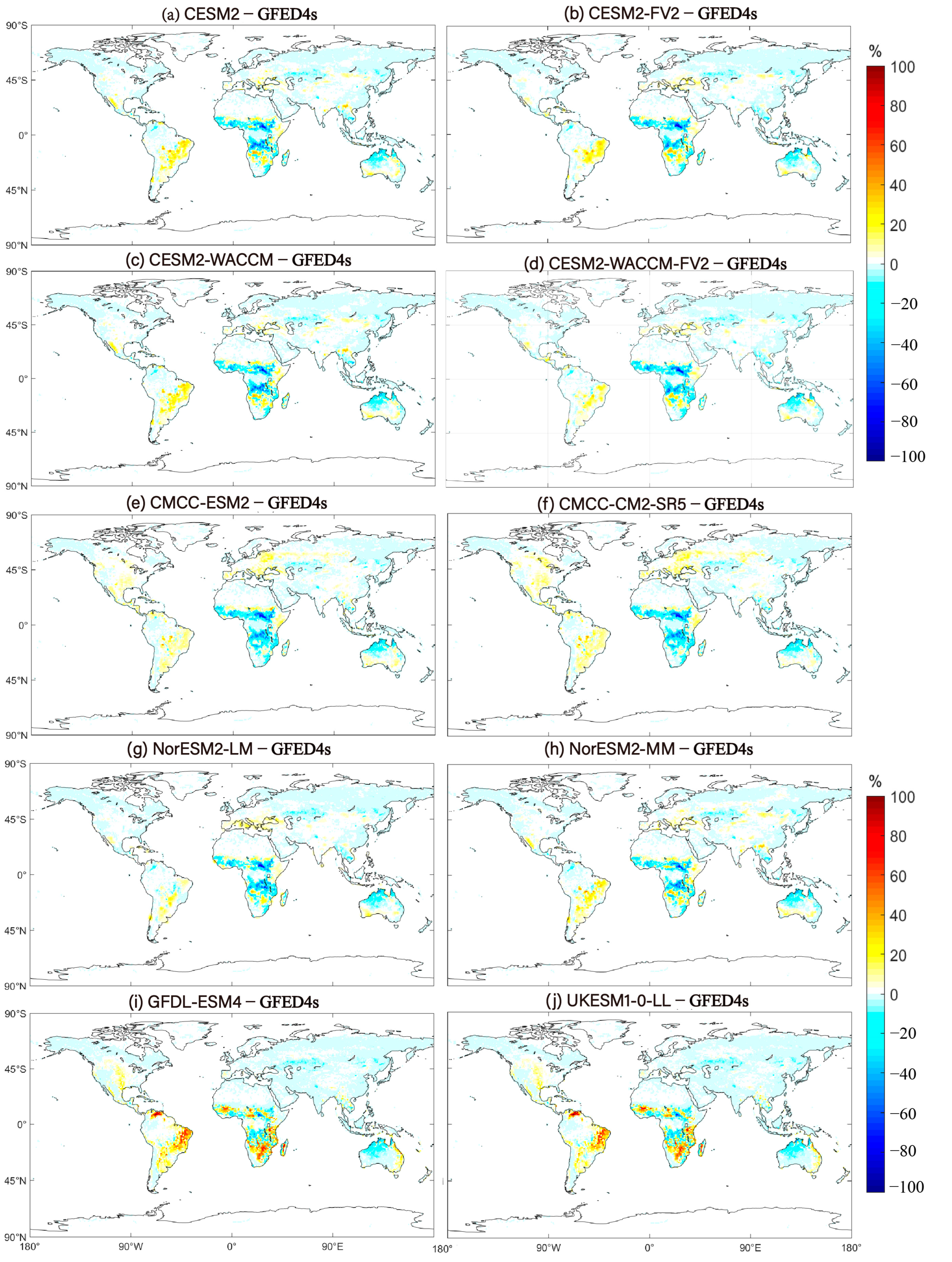
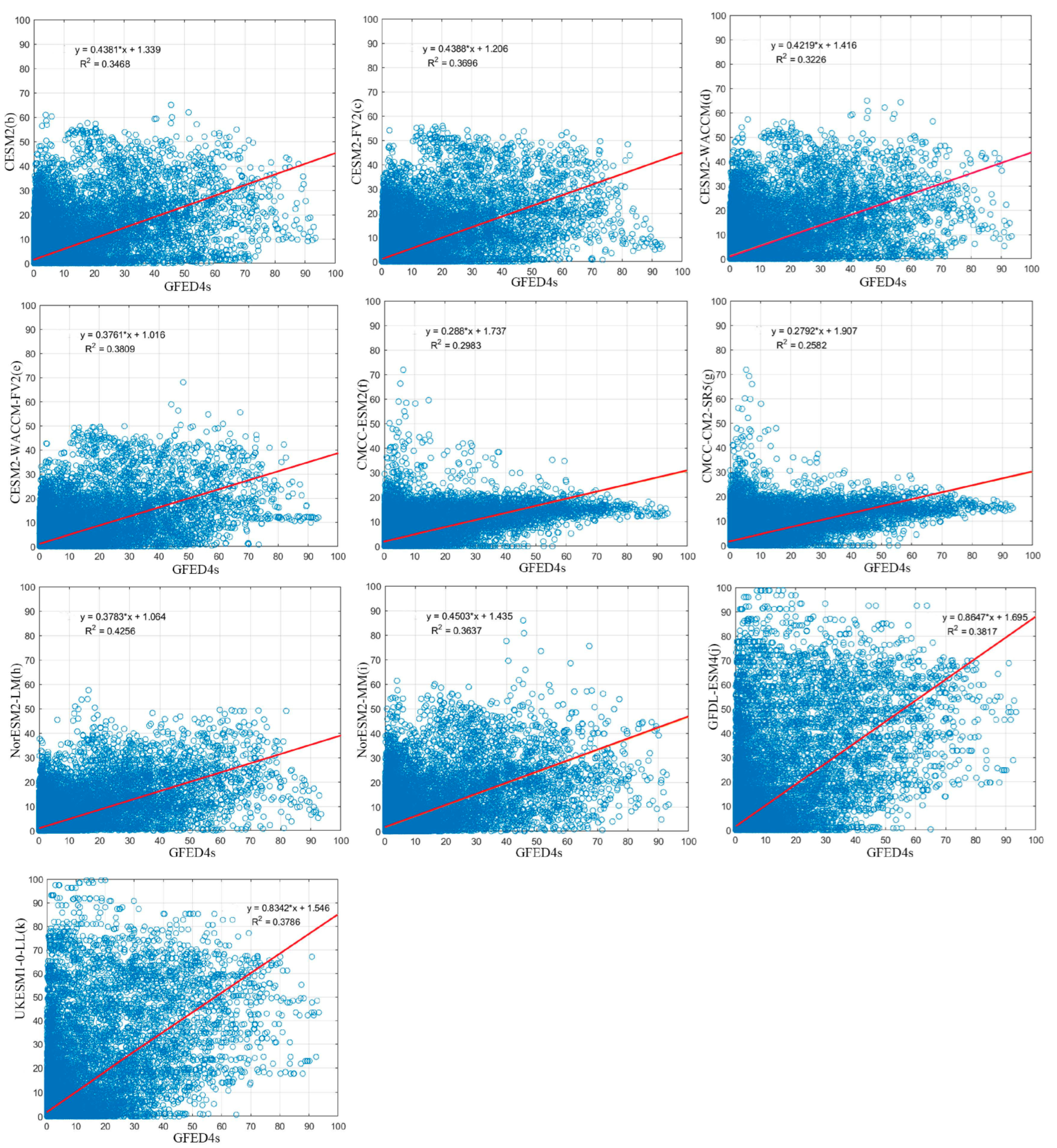
3.1. Evaluation of Historical Fire BA Simulation

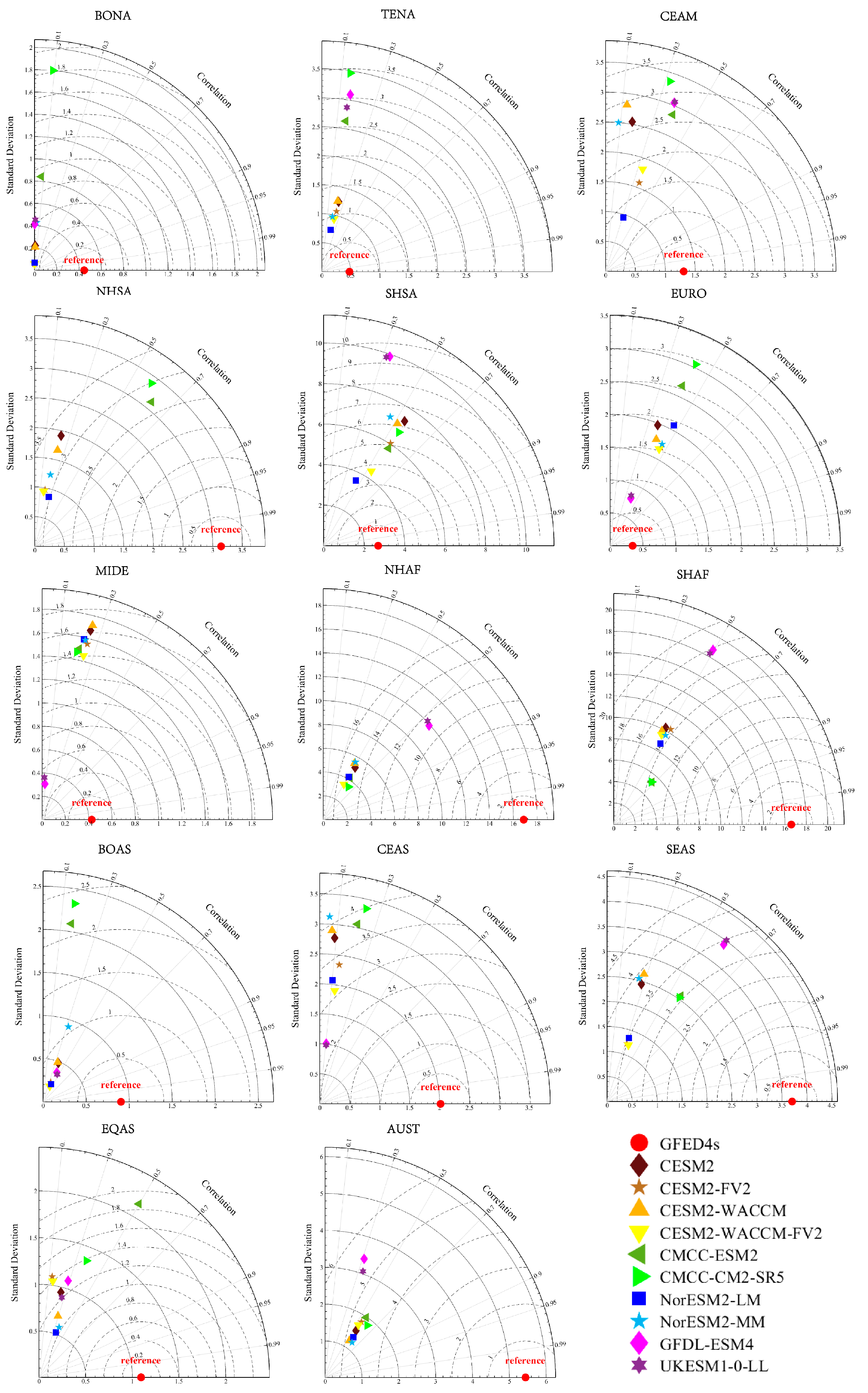
3.1.1. Annual Assessment

Figure 2 shows the spatial distribution of the differences between the simulated and referred annual BA fraction (BAF) for the different GCMs from 1997 to 2014. The reference BA was from GFED4s. The BAF was calculated by dividing the BA by the grid area in each grid cell. The underestimated areas (blue) simulated by the models were mainly located in Africa, northern Australia, and Eurasia, while the overestimated areas (yellow and red) were primarily found in eastern South America and parts of Africa.

Figure 2. Spatial distribution of the differences between the simulated and referred annual BA fractions (BAFs) from 1997 to 2014.

The differences between models were significant. For instance, the two BA datasets for GFDLESM4 (j) and UKESM1-0-LL (k) were more significantly overestimated in eastern South America and south-central Africa compared to other models, which exhibited moderate overestimation in eastern South America and significant underestimation in central and southeastern Africa. Overall, the eight models from CMIP6 (b–i) were generally underestimated compared to the GFED4s reference data, while the two ISIMIP3b datasets (j, k) tended to be more markedly overestimated. The specific biases of annual average BAFs for the different regions between models and GFED4s are shown in Table 3.

Table 3. The bias of annual average BAFs for the different regions between models and GFED4s (unit: %).

	Model	(b–a)	(c–a)	(d–a)	(e–a)	(f–a)	(g–a)	(h–a)	(i–a)	(j–a)	(k–a)
Region
BONA		−0.120	−0.156	−0.123	−0.155	0.293	0.675	−0.150	−0.063	−0.031	0.004
TENA		0.490	0.539	0.679	0.376	2.261	2.968	0.230	0.517	2.674	2.512
CEAM		2.230	1.543	2.493	2.260	3.356	3.585	1.049	1.946	2.018	1.885
NHSA		−0.125	−0.432	−0.275	−0.238	1.927	2.385	−0.516	−0.729	10.176	9.676
SHSA		4.663	4.220	4.921	2.805	3.170	3.923	2.057	4.441	8.402	7.130
EURO		0.156	0.514	0.459	0.485	1.178	1.324	0.783	0.546	0.142	0.167
MIDE		0.443	0.458	0.471	0.427	0.306	0.286	0.502	0.466	−0.062	−0.057
NHAF		−4.377	−5.378	−4.315	−6.011	−5.466	−5.602	−4.119	−3.694	1.481	1.045
SHAF		−4.604	−2.815	−4.384	−5.819	−8.980	−9.232	−6.773	−3.850	8.077	7.032
BOAS		−0.257	−0.388	−0.271	−0.410	0.536	0.750	−0.380	−0.012	−0.302	−0.321
CEAS		−0.120	−0.156	−0.123	−0.155	0.293	0.675	−0.150	−0.063	−0.031	0.004
SEAS		0.296	−0.510	0.216	−0.578	0.234	−0.066	−0.046	0.400	0.026	0.074
EQAS		−0.136	0.075	−0.295	0.042	0.520	0.075	0.111	−0.130	−0.049	−0.236
AUST		−2.044	−2.331	−2.351	−2.148	−2.206	−2.903	−2.858	−2.858	−2.231	−2.597

Figure 3 illustrates scatterplots of annual BAFs between ten models and the GFED4s and their fitted lines. A greater value of R² indicates a better simulation result. It is found that NorESM4LM (h) had the highest R² value of 0.4256, indicating the best fitness. In addition, GFDL-ESM4 (j), CESM2-WACCMFV2 (d), and UKESM1-0-LL (k) performed relatively well, with their R² values of 0.3817, 0.3809, and 0.3786, respectively. By contrast, CMCC-ESM2 (f) and CMCC-CM2-SR5 (g) had the worst R² values of 0.2983 and 0.2582, respectively, while those of the remaining four models fell within the range of 0.32–0.37.

Figure 3. Scatterplots of the linear relationship between the simulated and observed BAFs. The red lines represent the regression lines.

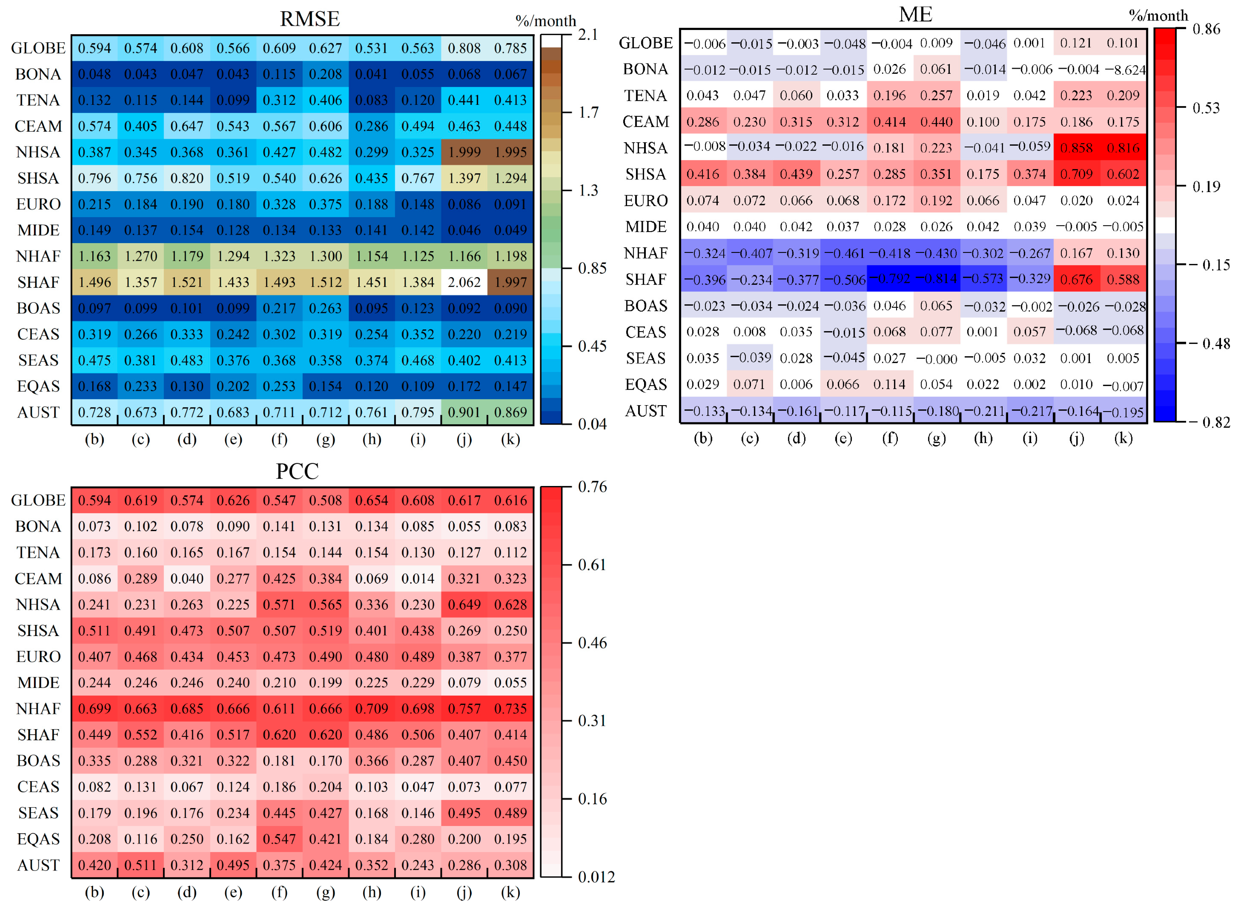
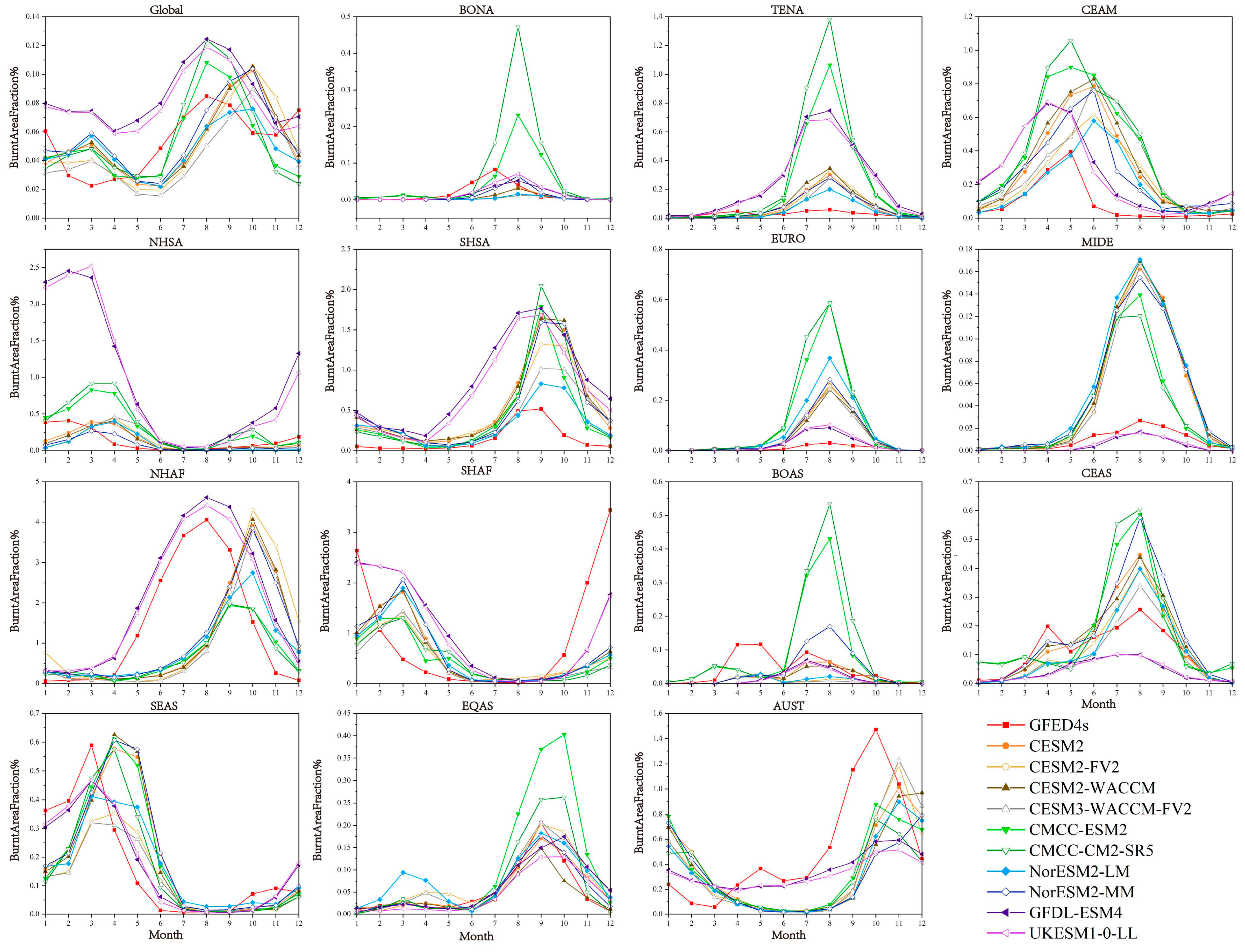
3.1.2. Monthly Assessment

Figure 4 presents statistical metrics, including RMSE, ME, and PCC, for the simulated and actual data on monthly averaged BAFs for the globe and its 14 subregions from 1997 to 2014.

Figure 4. Heatmap of statistical indicators of RMSE, ME, and PCC for the ten models for the globe and its 14 subregions.

On the global scale, the RMSE of the eight CMIP6 models (b–i) ranged from 0.53 to 0.63% per month. By contrast, the RMSE values for the two ISIMIP3b models (j, k) were 0.81 and 0.79% per month, significantly higher than those of the eight CMIP6 datasets. The ME values for ISIMIP models (j, k) were also much higher than those for the CMIP6 models (b–i). Among all models, NorESM2-LM (h) performed best, with the highest PCC of 0.654 and the lowest RMSE of 0.531% per month.

On the regional scale, the model performed better in terms of RMSE and ME in northern North America (BONA), the Middle East (MIDE), Northern Asia (BOAS), and EQAS. For PCC, the best performance was observed in Northern Hemisphere Africa (NHAF), followed by Southern Hemisphere Africa (SHAF).

Figure 5 illustrates the monthly average changes in BAFs for ten models and GFED4s for the globe and its 14 subregions. Globally, the GFED4s dataset showed low BA values from February to April and high BA values from July to September. However, all CMIP6 models exhibited a lag of 1–3 months, whereas the ISIMIP3b datasets aligned more closely with the reference data but with some significant deviations. Regionally, all models showed an overall higher bias in TENA, CEAM, SHSA, and EURO. Conversely, the models in SHAF (October–January), BOAS (April and May), and AUST regions (April–October) showed relatively low biases.

Figure 5. Monthly average variations in BAFs for ten models and GFED4s for the globe and its 14 subregions.

Among the different models, NorESM2-LE performed best in BUNA, TENA, CEAM, SHSA, and EQAS, while CMCC-ESM2 and CMCC-CM2-SR5 performed best in NHSA, SHAF, SEAS, and AUST. GFDL-ESM4 and UKESM1-0-LL from ISIMIP2b showed strong performance in EURO, MIDE, NHAF, BOAS, CEAS, and EQAS.

3.1.3. Seasonal Assessment

The fire season was defined as the months when values exceeded the average of all months. The fire seasons of ten models for the global subregions were quantified based on multi-year monthly averages of both models (Figure 5). The results are shown in Table 4. It was found that the fire seasons for the different regions were different. It was mainly divided into three categories: the first was mainly October–April, such as NHAF and AUST; the second was mainly from January to June, such as CEAM, NHSA, and SEAS; and the other categories were mainly distributed from June to October.

Table 4. The fire seasons of 14 regions for ten models and GFED4s.

	Model	GFED4s	(b)	(c)	(d)	(e)	(f)	(g)	(h)	(i)	(j)	(k)
Region
BONA		6–8	7–9	7–10	7–9	7–10	7–9	7–9	6–10	6–9	6–10	6–9
TENA		3–4, 7–9	7–9	7–10	7–10	7–10	7–9	7–9	7–9	6–10	6–10	6–10
CEAM		3–5	4–7	4–8	3–7	4–8	4–8	4–8	4–8	3–7	2–6	2–6
NHSA		12–3	1–5	2–5	2–5	2–5	1–5	1–5	2–5	2–5	1–4	1–4
SHSA		7–10	8–11	8–11	8–11	8–11	8–10	8–10	8–11	8–11	7–11	7–11
EURO		7–10	7–9	7–9	7–9	7–9	7–9	7–9	7–9	7–9	6–9	6–9
MIDE		6–10	7–10	7–10	7–10	7–10	6–9	6–9	6–10	6–10	7–10	6–10
NHAF		11–2	12–4	12–4	12–4	1–4	12–3, 5	1–5	1–4	12–4	12–4	12–4
SHAF		6–10	9–11	9–12	9–11	9–11	8–11	8–11	8–11	8–11	6–10	6–19
BOAS		4–5, 7–8	4, 7–9	4–5, 8–9	4–5, 7–9	4–5, 8	7–8	7–9	4–5, 7–9	7–9	6–9	6–8
CEAS		4–9	6–9	6–9	6–9	6–9	6–9	7–9	7–10	4–9	5–9	5–9
SEAS		1–4	2–6	1–5	2–5	1–5	2–5	2–5	1–6	2–6	1–5	1–5
EQAS		8–10	9–10, 12	8–11	8–10	8–11	8–11	8–10	3–4, 8–11	8–11	8–11	8–11
AUST		8–11	10–2	10–2	10–2	10–1	10–2	10–2	10–2	10–2	8–1	9–1

Figure 6 presents Taylor diagrams for the BAFs of the fire seasons simulated by ten models in the 14 regions. The reference data were obtained from the GFED4s. The results indicated that UKESM1-0-LL and GFDL-ESM4 stood out with better RMSE, PCC, and SD values in the regions of EURO, MIDE, BOAS, CEAS, and NHAF; CMCC-ESM2 and CMCC-CM2-SR5 performed better in the regions of SHSA, SHAF, SEAS, and AUST; and NorESM2-LM, CESM2-WACCM-FV2, and CESM2-FV2 performed better in the remaining regions. Overall, the better performances of the ten models based on Taylor diagrams are listed in Table 5. It is found that the simulation performance varied in the different regions, indicating the need to select different models in different regions for improvement in the future.

Figure 6. Taylor diagrams for the BAFs of fire seasons simulated by ten models in the 14 regions, where the reference data are GFED4s.

Table 5. The better performance of the ten models based on Taylor diagrams.

Region	Better Models
BONA	(b)(c)(d)(e)(h)(i)(j)(k)
TENA	(b)(c)(e)(h)(i)
CEAM	(h)(c)(e)
NHSA	(h)(c)(e)
SHSA	(h)(c)(e)(f)
EURO	(j)(k)
MIDE	(j)(k)
NHAF	(h)(j)(k)
SHAF	(f)(g)
BOAS	(b)(c)(d)(e)(h)(j)(k)
CEAS	(j)(k)
SEAS	(c)(e)(f)(g)(h)
EQAS	(h)(i)
AUST	(b)(c)(d)(e)(f)(h)(i)(g)

3.1.4. Comparisons of Global BAF Classes

Table 6 presents the percentages of global grids for three types of BAF classes across ten models. For consistent comparison, all data were uniformly interpolated onto a grid with a resolution of 0.5° × 0.5°. It was found that over 90% of grids for all models exhibited small fires (<1%), indicating that the small fires occurred with the highest frequency.

Table 6. Comparisons of the BAF across the ten GCMs for various fire rankings *.

Model	<1%	<2%	2~5%	5~10%	10–50%	>50%
GFED4s (a)	93.828%	95.559%	1.840%	0.931%	1.455%	0.215%
CESM2 (b)	92.810%	94.507%	2.085%	1.407%	1.971%	0.029%
CESM2-FV2 (c)	92.948%	94.558%	2.195%	1.352%	1.873%	0.021%
CESM2-WACCM (d)	92.803%	94.494%	2.010%	1.458%	2.020%	0.018%
CESM2-WACCM-FV2 (e)	93.181%	94.799%	2.218%	1.395%	1.586%	0.003%
CMCC-ESM2 (f)	90.540%	92.435%	3.007%	2.469%	2.086%	0.004%
CMCC-CM2-SR5 (g)	90.394%	92.262%	2.917%	2.480%	2.338%	0.003%
NorESM2-LM (h)	91.371%	93.772%	2.801%	1.858%	1.567%	0.002%
NorESM2-MM (i)	91.647%	93.728%	2.537%	1.727%	1.979%	0.029%
GFDL-ESM4 (j)	93.437%	94.608%	1.637%	1.164%	2.025%	0.566%
UKESM1-0-LL (k)	93.580%	94.824%	1.645%	1.133%	1.877%	0.522%

* Values in bold represent the results closer to GFED4s.

Compared to GFED4s, the BAF for CESM2-WACCM-FV2 (e), GFDL-ESM4 (j), and UKESM1-0-LL (k) were closer than other models for small fires (<2%). For small fires (2~10%), GFDL-ESM4 (j) and UKESM1-0-LL (k) outperformed the other models. For medium fires (10–50%), CESM2-WACCM-FV2 (e) was closest to GFED4s. However, there was a significant difference for all models concerning large fires (>50%). For instance, GFDL-ESM4 (j) and UKESM1-0-LL (k) showed a notable overestimation, exceeding 0.5% compared to GFED4s, which had a BAF of 0.215%. By contrast, the other model showed a large underestimation, with values below 0.03%.

3.2. Multi-Model Ensemble for Historical Fire BA Simulations

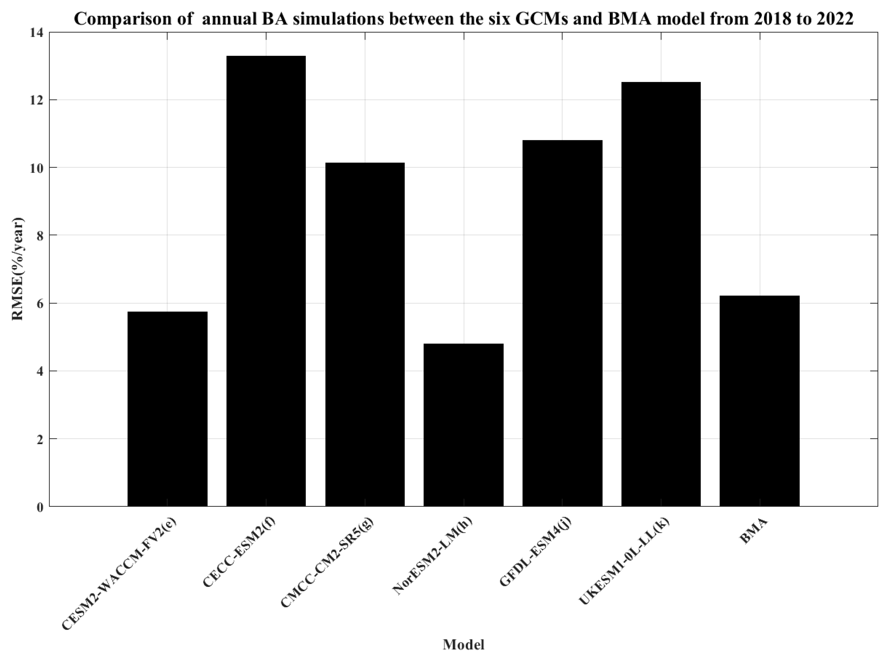
3.2.1. Model Ranking and Screening

Based on the results of the previous model evaluation analysis, Figure 7 presents the overall performance rankings of the ten models in terms of fire BA. Red represents the highest rankings, while blue indicates the lowest. On a global scale, the top-performing models were NorESM2-LM and CESM2-WACCM-FV2. However, the rankings of the same model varied significantly across different regions. For instance, NorESM2-LM performed well in most regions, but it ranked lower in EURO (R6), MIDE (R7), and NHAF (R8). Additionally, the ISIMIP datasets (GFDL-ESM4 and UKESM1-0-LL) ranked low both globally and across eight regions, yet they achieved first or second place in EURO (R6), MIDE (R7), NHAF (R8), BOAS (R10), and CEAS (R11). Based on the comprehensive ranking results for the globe and its 14 regions, six optimal models were selected: CESM2-WACCM-FV2, NorESM2-LM, CMCC-ESM2, CMCC-CM2-SR5, GFDL-ESM4, and UKESM1-0-LL.

Figure 7. Rank diagram of BA simulation capability on the monthly scale for all models for the globe and its 14 subregions: R1-R14 represent the regions of BONA, TENA, CEAM, NHSA, SHSA, EURO, MIDE, NHAF, SHAF, BOAS, CEAS, SEAS, EQAS, and AUSTR6, respectively.

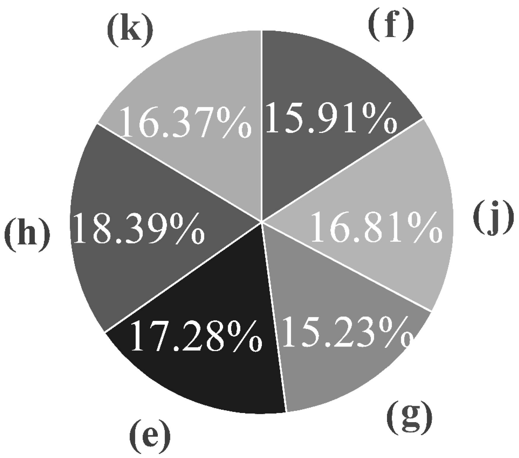
3.2.2. The Weights of Optimal Models and BMA Simulation

Based on the monthly GFED4s BA reference dataset, the six optimal models were assigned weights by the BMA method. The objective function for BMA was the RMSE of monthly BA from 1997 to 2014. Figure 8 shows the weight values of each selected model obtained through the BMA method. It indicates that NorESM2-LM (h) and CESM2-WACCM-FV2 (e) had the highest weights, at 18.39 and 17.28%, respectively. By contrast, the weights of other optimal models were relatively low. For example, the weights for GFDL-ESM4 (j), UKESM1-0-LL (k), CECC-ESM2 (f), and CMCC-CM2-SR5 (g) were 16.91, 16.37, 15.91, and 15.23%, respectively. Additionally, the Taylor diagram in Figure 9 demonstrates that the BMA multi-model ensemble provided superior results compared to individual models.

Figure 8. Weighting pie chart for the selected models based on monthly GFED4s BA dataset and BMA method: (f) CECC-ESM2, (j) GFDL-ESM4, (g) CMCC-CM2-SR5, (e) CESM2-WACCM-FV2, (h) NorESM2-LM, and (k) UKESM1-0-LL.

Figure 9. Taylor diagram of BA metrics for the ten models and BMA model.

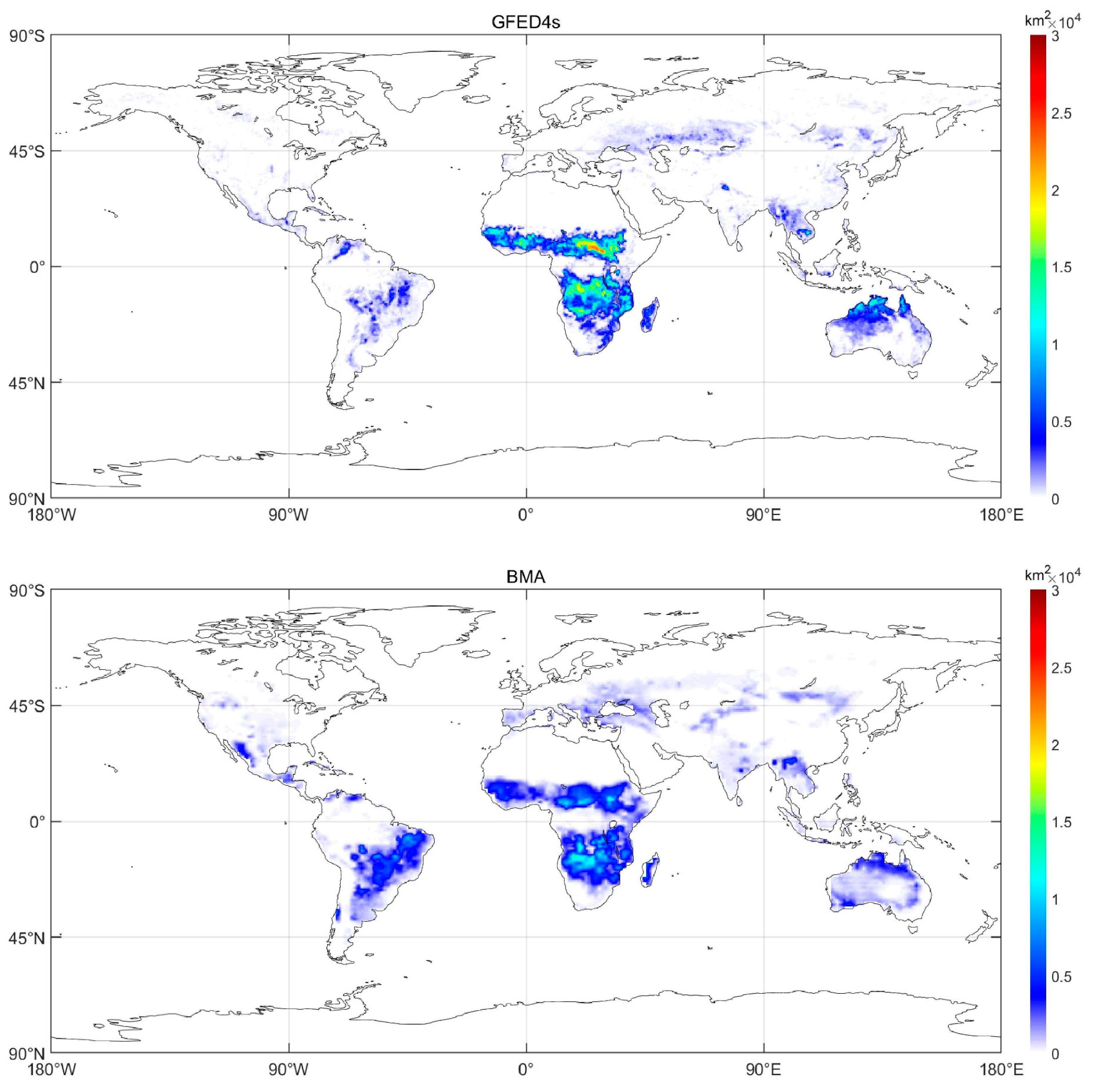
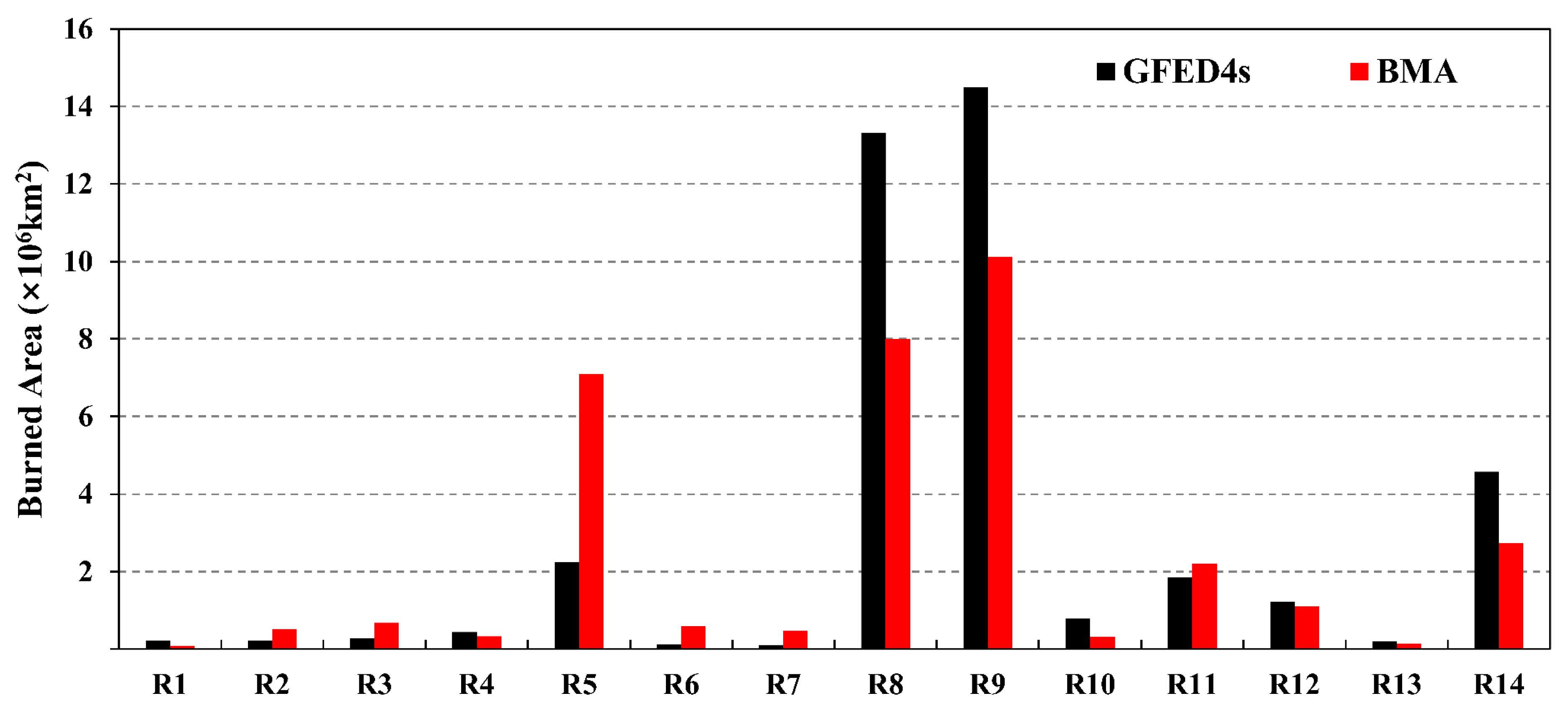
3.2.3. Spatial Comparison of Monthly BA Between BMA Model and GFED4s

Figure 10 illustrates the spatial distribution comparisons of monthly BA between the BMA model and GFED4s. The spatial distributions were generally similar, but there were some differences. For instance, BMA underestimated BA in Africa and northern Australia compared with GFED4s, while it overestimated BA in South America. Overall, the differences between the two were more pronounced in the Southern Hemisphere than in the Northern Hemisphere.

Figure 10. Spatial distribution comparisons of monthly BA between BMA model and GFED4s.

Figure 11 illustrates the monthly BA across different regions as provided by two datasets from GFED4s and BMA. It is evident that the average monthly BA in the African regions (R8 and R9) was highest in both GFED4s and BMA, with values of 27.83 × 10⁶ and 18.11 × 10⁶ km², respectively. The BA in AUST (R14) was 1.84 × 10⁶ km² lower than that of GFED4s. By contrast, BMA showed a BA 4.85 × 10⁶ km² higher than that of GFED4s in SHSA (R5). Except for R5, R8, R9, and R14, other regions demonstrated a lower BA (<2 × 10⁶ km²) for both GFED4s and BMA. The BA of the BMA model represented underestimation in the top three areas with the highest BA. This was consistent with the results shown in Figure 10.

Figure 11. Bar charts of monthly BA across different regions for the BMA model and GFED4s, where R1-R14 represent the regions of BONA, TENA, CEAM, NHSA, SHSA, EURO, MIDE, NHAF, SHAF, BOAS, CEAS, SEAS, EQAS, and AUSTR6, respectively.

3.3. Future Fire BA Prediction Based on the BMA Model

3.3.1. Validation of the Projections for the 2015–2040 Period

A new fire year from 2015 to 2040 was selected to validate the effectiveness of BMA ensemble simulations constructed from the historical BA dataset covering the period from 1997 to 2014. Figure 12 shows a comparison of annual BA simulations between six selected GCMs and the BMA model from 2018 to 2022. For the six models, it is evident that CESM2-WACCM-FV2 (e) and NorESM2-LM (h) demonstrated better performance than the others, with RMSE values of 5.74%/year and 4.82%, respectively. Notably, they were assigned higher weights in BMA for historical simulations.

Figure 12. Comparison of annual BA simulations in 2022 between six selected GCMs and BMA models from 2018 to 2022.

For the other models, UKESM1-0L-LL (k) had an RMSE of 12.51%/year, while CECC-ESM2 (f), CMCC-CM2-SR5 (g), and GFDL-EMS4 (j) exhibited RMSE values of 13.28, 10.14, and 11.81%/year, respectively. Overall, BMA demonstrated the best simulation performance among the six models, achieving an RMSE value of 6.32%/year. Clearly, the effectiveness of BMA was further validated in the BA projections for the 2015–2040 period.

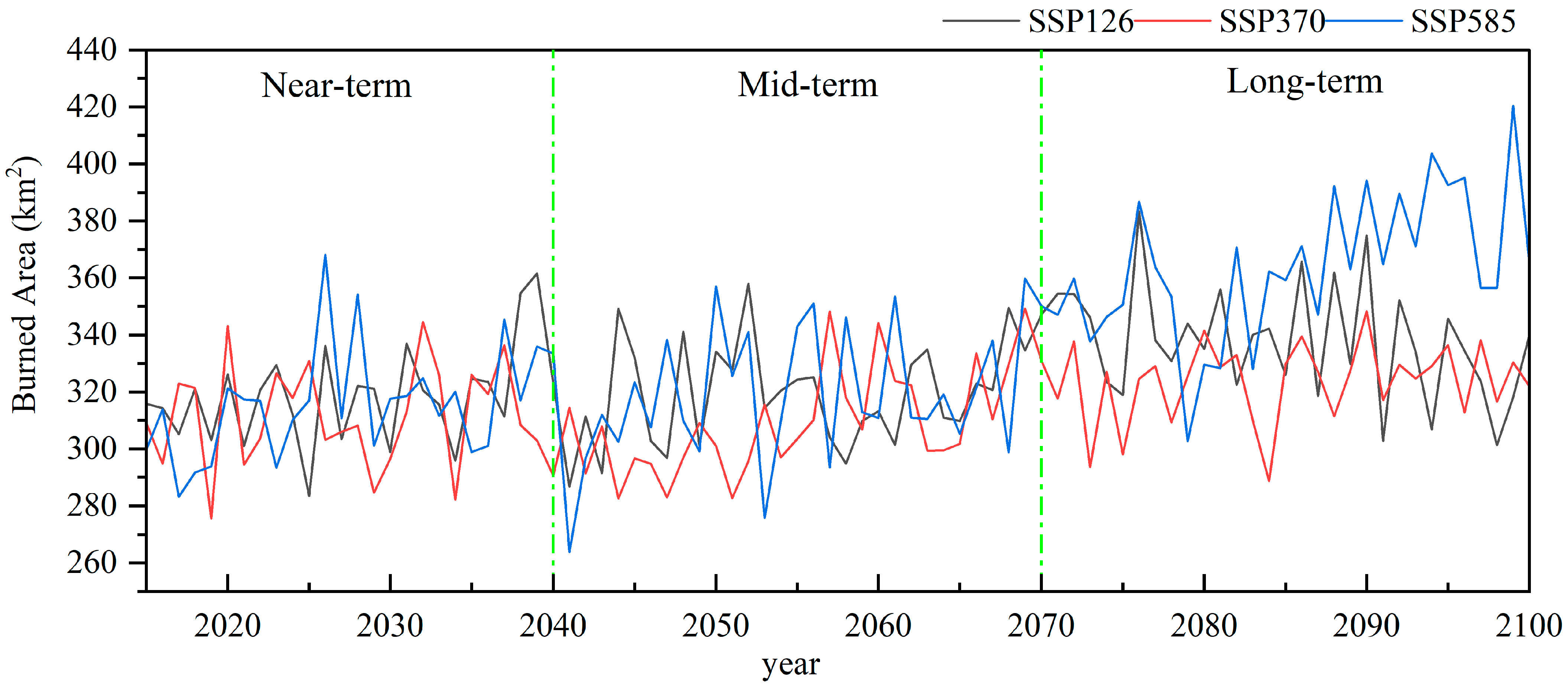
3.3.2. Future Temporal Changes in the Annual BA Under Different Scenarios

Based on the weighting of the BMA model and the future predictions of its members, the global BA ensemble forecast results were generated for the future. Figure 13 shows the annual changes in the BA predicted by the BMA model under three scenarios (SSP126, SSP370, and SSP585) for the near (2015 to 2040), mid (2041 to 2070), and long (2071 to 2100) term. The global BA showed an overall upward trend across the three scenarios. The annual BA increased by 0.32, 0.27, and 0.89 ${\mathrm{k}\mathrm{m}}^2$ per year on average under SSP126, SSP370, and SSP585, respectively.

Figure 13. The annual changes in BA under three scenarios (SSP126, SSP370, and SSP585) for the future from 2015 to 2100, including the near (2015 to 2040), mid (2041 to 2070), and long (2071 to 2100) terms.

In the three periods of the SSP126 scenario, the trend was first to increase and then to decrease, with changes of 0.85, 0.59, and −0.74 ${\mathrm{k}\mathrm{m}}^2$ per year, respectively. In the SSP370 scenario, the three periods all showed an increasing trend, with changes of 0.06, 1.00, and 0.35 ${\mathrm{k}\mathrm{m}}^2$ per year, respectively. Finally, in the SSP585 scenario, the three periods also showed a significant increase, with changes of 1, 0.98, and 2 ${\mathrm{k}\mathrm{m}}^2$ per year, respectively. It can be seen that the increasing trend in the SSP585 scenario was significantly higher than the growth trend in the SSP370 and SSP 126 scenarios.

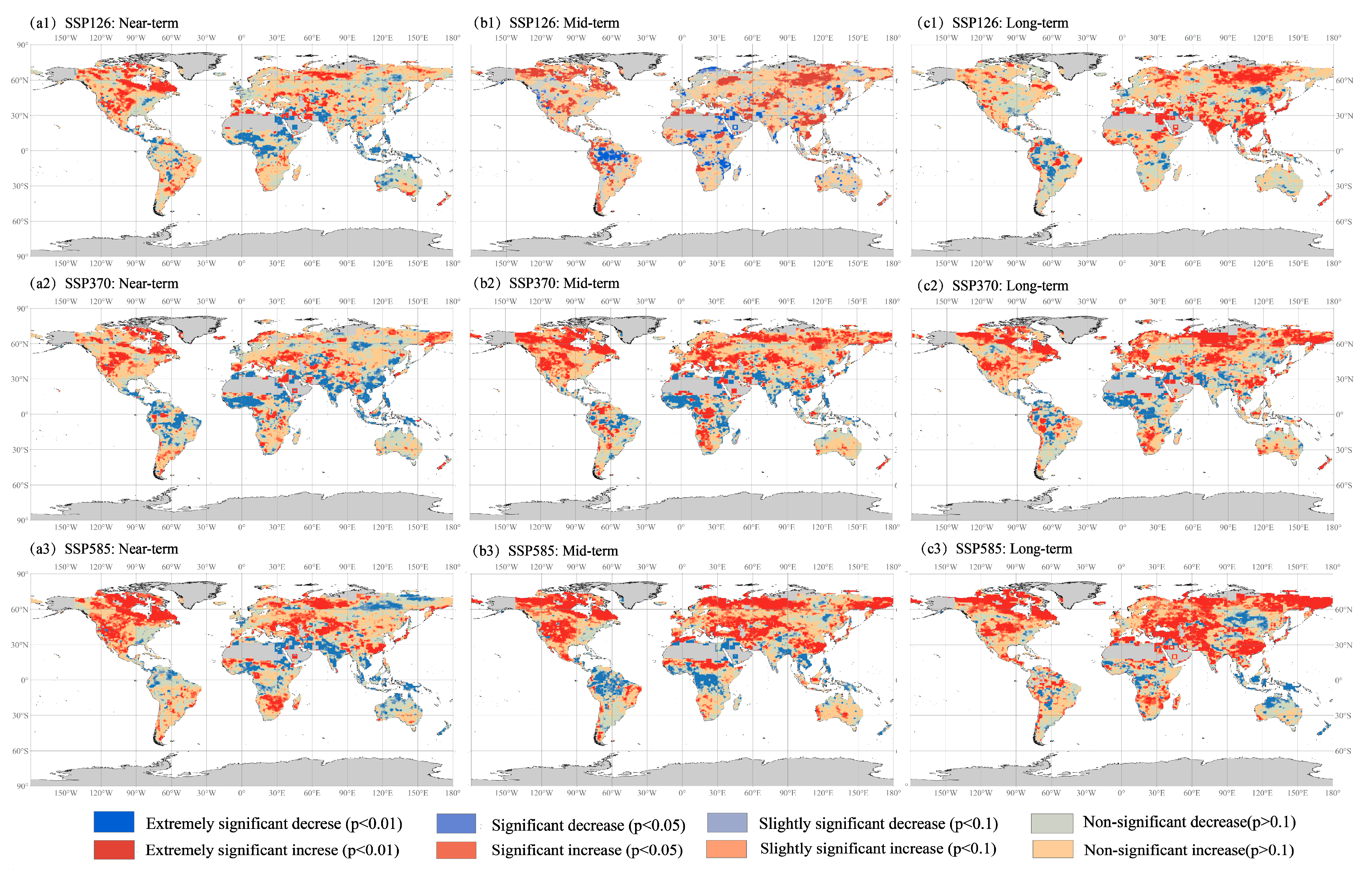
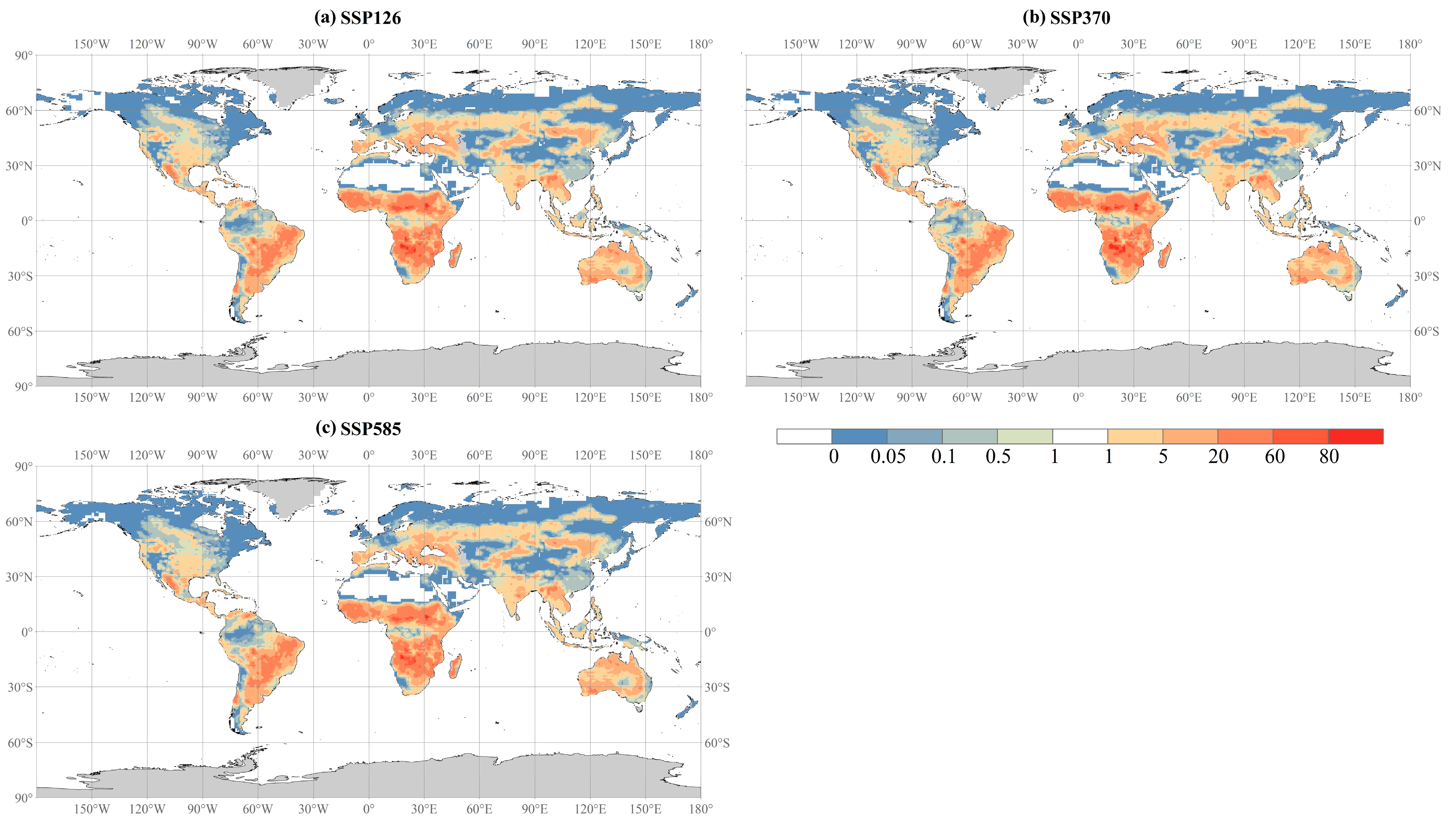
3.3.3. Future Spatial Changes in BA Under Different Scenarios

Figure 14 shows a spatial trend map of the average annual BA in three periods under three future scenarios based on the MK trend test. Red represents an increase in BA, and blue represents a decrease. They were divided into four levels: extremely significant (p < 0.01), significant (p < 0.05), slightly significant (p < 0.1), and insignificant (p > 0.1).

Figure 14. Spatial distributions of annual BA change trends across different periods under three future scenarios.

Under the SSP126 scenario, the BA showed a general upward trend in the near term worldwide, among which the areas with extremely significant increases (p < 0.01) were concentrated in North America and Northern and Western Asia, and the areas with significant decreases (p < 0.05) were mainly concentrated near the equator in Africa. In the mid-term of SSP126, there were extremely significant increases (p < 0.01) in the global BA, with a trend of shrinking in North America and increasing in Asia, and an extremely significant downward trend (p < 0.01) in northern South America. In the long term, for SSP126, the upward trend in North America weakened, and the extremely significant upward trend (p < 0.01) in Asia further strengthened.

In the near term of the SSP370 scenario, the BA showed a general upward trend above 30°N, with extreme increases (p < 0.1) primarily occurring between 30 and 60°N. Conversely, there was a significant downward trend (p < 0.05) between 30°S and 30°N. In the mid-term of SSP370, the extremely significant increase in area (p < 0.01) between 30 and 60°N expanded significantly, while the extremely significant decrease in area (p < 0.01) between 0 and 30°N decreased significantly. In the long term, for SSP370, the area with the extremely significant upward trend (p < 0.01) expanded further, and the area with the significant downward trend (p < 0.01) further decreased. In general, the BA in more and more areas will show an increasing trend in the future.

In the near, mid, and long term, in the SSP585 scenario, the extremely significant upward areas (p < 0.01) all showed a significant expansion, which was far larger than those of SSP126 and SSP370, respectively. It can be found from SSP126 to SSP307 to SSP585 that as the emission scenario intensifies, the BA areas will show extremely significant increases.

4. Discussion

4.1. Uncertainty Analysis of BA Under Different Scenarios

Figure 15 shows the spatial distribution of SN for uncertainty analysis of the global BA simulation under future scenarios. SN values less than 1 (blue) indicate uncertainty, while those greater than 1 (orange-red) indicate reliability.

Figure 15. Spatial distribution of SN for the uncertainty analysis of global BA simulation under three future scenarios, where blue indicates uncertainty and red indicates reliability. White represents the missing value.

It can be seen that the data credibility distributions of the three future scenarios were similar. Areas with higher uncertainty were mainly distributed near 60°N, in Central Asia, near the equator of South America, along the eastern coast of Australia, and in New Zealand. Areas with higher reliability were mainly distributed in Africa, South America, and most parts of Australia.

From SSP126 to SSP370, the reliability of the model was further strengthened in south-central Africa, western Australia, and eastern South America, while uncertainty decreased in northern South America. From SSP370 to SSP585, the uncertainty gradually increased in the north of South America, and the reliability weakened again in south-central Africa. Some regions are more prone to higher uncertainty due to climatic or land use variability, which could affect BA projections.

4.2. Uncertainty in Historical Simulation Results

The accuracy of model simulation results is primarily influenced by data gaps. Specifically, incomplete or inaccurate input data, particularly in situations where terrain monitoring is challenging or meteorological data coverage is inadequate, can lead to missing simulation results [41]. Uncertainty in parameter estimation within fire models also impacts simulation outcomes [42]. Research indicates that input uncertainty is high for fuel model parameters; therefore, these parameters need to be calibrated based on actual fire conditions, with a focus on those exhibiting significant spatiotemporal variability. Model resolution is another crucial factor affecting simulation capabilities [43]. High-resolution models can better capture small-scale physical processes and local features, leading to more accurate simulations and predictions of extreme events [44]. For instance, combining high-resolution simulations with low-resolution ensembles can improve the SN ratio, particularly in extreme precipitation simulations [45]. On the regional scale, increasing the model resolution enhances the representation of terrain variations, land use, and other factors, thereby improving the simulation of regional climate and weather events [46]. For BA simulations, a higher-resolution model enables the fire perimeter and shape to be estimated more accurately, with the accuracy of the estimation of the former directly affecting the accuracy of the BA assessment [47]. Additionally, the ability to simulate BA is affected by other factors, such as the characteristics of the combustible materials, meteorological conditions, and variations in human activities and social policies.

4.3. Effects of Different Land Cover Types

First, different land cover types have distinct reflection, absorption, and conduction properties, which directly impact the model’s ability to simulate energy balance and radiation processes [48]. Secondly, various land cover types exhibit different fuel characteristics, including vegetation type, density, and moisture content, which also affect the accuracy of BA simulation [49,50]. For example, the Indian Forest Survey found that areas with 6% forest coverage in the country are more prone to fires [51]. These fuel characteristics directly influence the difficulty of fire ignition and the spread of fire [52]. Additionally, land cover types play a crucial role in fire risk assessment and management. Different land cover types have varying flammability and fire potential [53,54], which are significant for fire prevention, monitoring, and disaster management. Therefore, accurate land cover data are essential for enhancing the model’s BA simulation capabilities.

4.4. Selection of Different Assessment Methods

Different fire evaluation methods and metrics can result in varying outcomes in model ranking. This study primarily assessed and ranked model simulation capabilities using common statistical metrics, including RMSE, ME, and PCC, and Taylor indices. Some studies have developed new methods for model evaluation. For example, Desmet et al. [55] used a scoring function that exhibits exponential growth in performance, while Khadka et al. [56] employed multi-criteria decision making to rank model simulations of Southeast Asian atmospheric circulation. In wildfire model evaluation, some studies have highlighted the assessment of fire risk by calculating and determining global or regional fire risk using a combination of static and dynamic indices [57,58]. Additionally, other research evaluated the ability of models to simulate fire weather conditions by calculating fire weather indices based on simulated wind speed, wind direction, relative humidity, and temperature [26,32]. Therefore, the selection of different evaluation methods and metrics may also significantly influence the resulting model rankings.

4.5. Future Implications of BA Increases

It has been observed that the global BA exhibits an overall upward trend across the three future scenarios, particularly under high-emission scenarios such as SSP585. Increases in BA would have significant implications for potential ecological and socioeconomic impacts.

As BA increases, there will be a corresponding rise in the frequency and intensity of fires, shifts in vegetation types [59], and loss of biodiversity [60]. For example, fire-adapted species may proliferate while more sensitive species decline, thereby altering local biodiversity. Many species are at risk of extinction due to the severe widespread fires, particularly in vulnerable ecosystems such as tropical forests and grasslands [61]. Increased BA may also lead to shifts in animal populations, disrupting predator–prey dynamics and resulting in species imbalances. Species that rely on specific habitats may face increased competition and reduced survival rates.

Increasing BA would also have several socioeconomic implications. For instance, increased BA leads to higher levels of air pollution, posing serious health risks for populations living near fire-prone areas. This could result in a rise in respiratory diseases and cardiovascular issues, placing additional strain on public health systems. In addition, as BA increases, agricultural land may be lost or degraded, negatively impacting food production and resulting in severe economic losses for farmers. This is particularly concerning in regions already vulnerable to climate variability, which could lead to increased food prices and potential shortages. Finally, an increase in BA also has implications for insurance and risk management. As wildfire risks escalate, insurance premiums may be at risk, making it more difficult for homeowners and businesses to secure coverage. At the same time, to mitigate the disaster risk, greater investment will be required for firefighting and emergency response services, further increasing the burden of social risk costs.

Consequently, effective fire management and policy measures will be necessary in the future, especially for high-risk fire regions. For instance, policymakers must develop adaptive fire management strategies that account for the potential increase in BA. This includes developing firebreaks, enhancing vegetation management, or implementing controlled burns to reduce fuel load. Investment in monitoring systems can also help track changes in BA and inform adaptive management practices. Additionally, educating communities about the risks associated with increased BA, developing community training programs, and establishing local fire response teams will foster greater community resilience.

4.6. Potential Limitations of GCMs and Satellite Data for BA Projections

Several potential limitations should be noted when utilizing GCMs and satellite data for BA projections. The first limitation is the issue of resolution. GCMs typically operate at coarser spatial resolutions, often on the order of 100 km or more, which can obscure localized variations in climate and land use that significantly affect fire dynamics. Similarly, satellite data may also be limited in spatial resolution and temporal frequency, leading to gaps in our understanding of fire occurrence and intensity at finer scales, particularly in heterogeneous landscapes characterized by dense vegetation or a complex topography. Another limitation is the lack of consideration for local fire management practices. GCMs and satellite data primarily focus on climate and vegetation dynamics but often do not account for local fire management practices. Practices including controlled burning, fire suppression strategies, and community engagement in fire risk management can greatly influence fire regimes. Without integrating these local strategies, projections may not accurately reflect the BA, resulting in either overestimations or underestimations of fire risk. Therefore, integrating higher-resolution local models and incorporating fire management practices are crucial steps towards more effective BA prediction as well as improved fire risk assessments and management strategies.

5. Conclusions

This study analyzed the spatiotemporal variations in global fire BA over a century (from 1997 to 2100) using the data from ten global fire models and one satellite fire product. The history simulations spanned from 1997 to 2014, while the future predictions were divided into three stages, near (2015–2040), mid (2041–2070), and long (2071–2100) term, based on three different SSPs. The satellite fire product GFED4s was used to evaluate the BA simulations from eight CMIP6 models and two ISIMIP models. Finally, six of the ten models were selected and weighted to obtain an optimal ensemble average simulation, which was then used to predict future variations in global BA. The main conclusions are as follows:

On an annual scale, the eight CMIP6 models generally exhibited a more pronounced underestimation compared to the GFED4s reference data, while the two ISIMIP3b models showed a clearer overestimation. On a monthly scale, the BAF simulations for the eight CMIP6 models were lower than those of the two ISIMIP3b models. Although the two ISIMIP3b models had the highest PCC, they also exhibited the most significant overestimation. NorESM2-LM from CMIP6 showed the best monthly BA simulation result, achieving the highest PCC of 0.654 and the lowest RMSE of 0.531% per month.

In the comparisons of global BA rank grid proportion, CESM2-WACCM-FV2 and NorESM2-LM overestimated the proportion of small fires (BA ≤ 10%) in global grids, while other models underestimated this proportion. For medium fires (10% < BA < 50%), all models showed a higher proportion of grids than the reference dataset. In the case of large fires (BA ≥ 50%), GFDL-ESM4 and UKESM1-0-LL from ISIMIP3b significantly overestimated the proportion of grids, while the other models tended to underestimate it.

Through multi-model comparisons across all seven regions, six models were selected: CESM2-WACCM-FV2, NorESM2-LM, CMCC-ESM2, CMCC-CM2-SR5, GFDL-ESM4, and UKESM1-0-LL. Each model was assigned a different weight based on the BMA method and GFED4s dataset. Among these, NorESM2-LM and NorESM2-LM received the highest weights, at 18.39 and 17.28%, respectively. The metrics indicated that the BMA model outperformed each individual model. While the spatial distributions of the two models were quite similar globally, some differences were observed. For instance, the BA from BMA was underestimated in Africa and northern Australia, while it was overestimated in South America. Overall, the differences between the two models were pronounced in the Southern Hemisphere compared to the Northern Hemisphere.

Under the SSP126 scenario, the temporal trend showed an initial increase followed by decreases across the three periods. In the SSP370 scenario, there was a continuous upward trend in all three periods, while in the SSP585 scenario, the continuous increasing trends were further amplified across all three periods. It can be observed that as the emission scenarios progress from SSP126 to SSP370 and then to SSP585, the area experiencing a significant increase in BA will expand considerably. The reliability distributions of the ensemble predictions for the three future scenarios were similar, and a highly reliable prediction was achieved for most regions. Regions of high uncertainty were located at latitudes above 60°N, as well as in Central Asia, near the equator in South America, along the eastern coast of Australia, and in New Zealand. By contrast, areas with a higher reliability were found in Africa and South America.

References

- Richardson, D.; Black, A.S.; Irving, D.; Matear, R.J.; Monselesan, D.P.; Risbey, J.S.; Squire, D.T.; Tozer, C.R. Global increase in wildfire potential from compound fire weather and drought. npj Clim. Atmos. Sci. 2022, 5, 23. [Google Scholar] [CrossRef]
- Cunningham, C.X.; Williamson, G.J.; Bowman, D.M.J.S. Increasing frequency and intensity of the most extreme wildfires on Earth. Nat. Ecol. Evol. 2024, 8, 1420–1425. [Google Scholar] [CrossRef] [PubMed]
- Bedia, J.; Herrera, S.; Gutiérrez, J.M.; Benali, A.; Brands, S.; Mota, B.; Moreno, J.M. Global patterns in the sensitivity of burned area to fire-weather: Implications for climate change. Agric. For. Meteorol. 2015, 214, 369–379. [Google Scholar] [CrossRef]
- Zheng, B.; Ciais, P.; Chevallier, F.; Chuvieco, E.; Chen, Y.; Yang, H. Increasing forest fire emissions despite the decline in global burned area. Sci. Adv. 2021, 7, eabh2646. [Google Scholar] [CrossRef]
- Chen, Y.; Morton, D.C.; Randerson, J.T. Remote sensing for wildfire monitoring: Insights into burned area, emissions, and fire dynamics. One Earth 2024, 7, 1022–1028. [Google Scholar] [CrossRef]
- Coop, J.D.; Parks, S.A.; Stevens-Rumann, C.S.; Ritter, S.M.; Hoffman, C.M. Extreme fire spread events and area burned under recent and future climate in the western USA. Glob. Ecol. Biogeogr. 2020, 31, 1949–1959. [Google Scholar] [CrossRef]
- David, E.C.; Krista, M.G.; Greg, J.; Ronald, P.N. Forest Service Large Fire Area Burned and Suppression Expenditure Trends, 1970–2002. J. For. 2005, 103, 179–183. [Google Scholar] [CrossRef]
- Lydersen, J.M.; Collins, B.M.; Brooks, M.L.; Matchett, J.R.; Shive, K.L.; Povak, N.A.; Kane, V.R.; Smith, D.F. Evidence of fuels management and fire weather influencing fire severity in an extreme fire event. Ecol. Appl. 2017, 27, 2013–2030. [Google Scholar] [CrossRef]
- Wang, Y.; Gao, F.; Li, M. Probabilistic path planning for UAVs in forest fire monitoring: Enhancing patrol efficiency through risk assessment. Fire 2024, 7, 254. [Google Scholar] [CrossRef]
- Giglio, L.; Boschetti, L.; Roy, D.P.; Humber, M.L.; Justice, C.O. The Collection 6 MODIS burned area mapping algorithm and product. Remote Sens. Environ. 2018, 217, 72–85. [Google Scholar] [CrossRef] [PubMed]
- Copernicus Climate Change Service, Climate Data Store, 2019. Fire Burned Area from 2001 to Present Derived from Satellite Observation. Copernicus Climate Change Service (C3S) Climate Data Store (CDS). Available online: https://cds.climate.copernicus.eu/datasets/satellite-fire-burned-area?tab=overview (accessed on 11 March 2023).
- Van Der Werf, G.R.; Randerson, J.T.; Giglio, L.; Van Leeuwen, T.T.; Chen, Y.; Rogers, B.M.; Mu, M.; van Marle, M.J.E.; Morton, D.C.; Collatz, G.J.; et al. Global fire emissions estimates during 1997–2016. Earth Syst. Sci. Data 2017, 9, 697–720. [Google Scholar] [CrossRef]
- Mangeon, S.; Field, R.; Fromm, M.; Mchugh, C.; Voulgarakis, A. Satellite versus ground-based estimates of burned area: A comparison between MODIS based burned area and fire agency reports over North America in 2007. Am. Polit. Sci. Rev. 2015, 72, 76–92. [Google Scholar] [CrossRef]
- Joshi, J.; Sukumar, R. Improving prediction and assessment of global fires using multilayer neural networks. Sci. Rep. 2021, 11, 3295. [Google Scholar] [CrossRef]
- Wang, X.; Di, Z.; Liu, J. Evaluating the Abilities of Satellite-Derived Burned Area Products to Detect Forest Burning in China. Remote Sens. 2023, 15, 3260. [Google Scholar] [CrossRef]
- Grishin, A.M.; Filkov, A.I. A deterministic-probabilistic system for predicting forest fire danger. Fire Saf. J. 2011, 46, 56–62. [Google Scholar] [CrossRef]
- Guyette, R.P.; Stambaugh, M.C.; Dey, D.C. Predicting Fire Frequency with Chemistry and Climate. Ecosystems 2012, 15, 322–335. [Google Scholar] [CrossRef]
- Baranovskii, N.V.; Kirienko, V.A. Ignition of Forest Combustible Materials in a High-Temperature Medium. J. Eng. Phys. Thermophy 2020, 93, 1266–1271. [Google Scholar] [CrossRef]
- Anderson, K. A model to predict lightning-caused fire occurrences. Int. J. Wildland Fire 2002, 11, 163–172. [Google Scholar] [CrossRef]
- Baranovskiy, N.V.; Kirienko, V.A. Forest Fuel Drying, Pyrolysis and Ignition Processes during Forest Fire: A Review. Processes 2022, 10, 89. [Google Scholar] [CrossRef]
- Wen, J.X. Fire modelling: The success, the challenges, and the dilemma from a modeller’s perspective. Fire Saf. J. 2024, 144, 104087. [Google Scholar] [CrossRef]
- Singh, H.; Ang, L.M.; Lewis, T.; Paudyal, D.; Acuna, M.; Srivastava, P.K.; Srivastava, S.K. Trending and emerging prospects of physics-based and ML-based wildfire spread models: A comprehensive review. J. For. Res. 2024, 35, 135. [Google Scholar] [CrossRef]
- Marcozzi, A.; Wells, L.; Parsons, R.; Mueller, E.; Linn, R.; Hiers, J.K. FastFuels: Advancing wildland fire modeling with high-resolution 3D fuel data and data assimilation. Environ. Modell. Softw. 2025, 183, 106214. [Google Scholar] [CrossRef]
- Eyring, V.; Bony, S.; Meehl, G.A.; Senior, C.A.; Stevens, B.; Stouffer, R.J.; Taylor, K.E. Overview of the Coupled Model Intercomparison Project Phase 6 (CMIP6) experimental design and organization. Geosci. Model Dev. 2016, 9, 1937–1958. [Google Scholar] [CrossRef]
- Hetzer, J.; Forrest, M.; Ribalaygua, J.; Prado-López, C.; Hickler, T. The fire weather in Europe: Large-scale trends towards higher danger. Environ. Res. Lett. 2024, 19, 084017. [Google Scholar] [CrossRef]
- Quilcaille, Y.; Batibeniz, F.; Ribeiro, A.F.S.; Padrón, R.S. Fire weather index data under historical and SSP projections in CMIP6 from 1850 to 2100. Earth Syst. Sci. Data 2023, 15, 2153–2177. [Google Scholar] [CrossRef]
- O’Neill, B.C.; Tebaldi, C.; van Vuuren, D.P.; Eyring, V.; Friedlingstein, P.; Hurtt, G.; Knutti, R.; Kriegler, E.; Lamarque, J.-F.; Lowe, J.; et al. The Scenario Model Intercomparison Project (ScenarioMIP) for CMIP6. Geosci. Model Dev. 2016, 9, 3461–3482. [Google Scholar] [CrossRef]
- Burton, C.; Lampe, S.; Kelley, D.I.; Thiery, W.; Hantson, S.; Christidis, N.; Gudmundsson, L.; Forrest, M.; Burke, E.; Chang, J.; et al. Global burned area increasingly explained by climate change. Nat. Clim. Chang. 2024, 14, 1186–1192. [Google Scholar] [CrossRef]
- Hantson, S.; Hamilton, D.S.; Burton, C. Changing fire regimes: Ecosystem impacts in a shifting climate. One Earth 2024, 7, 942–945. [Google Scholar] [CrossRef]
- Wang, T.; Tu, X.; Singh, V.P.; Chen, X.; Lin, K. Global data assessment and analysis of drought characteristics based on CMIP6. J. Hydrol. 2021, 596, 126091. [Google Scholar] [CrossRef]
- Kim, Y.; Min, S.; Zhang, X.; Sillmann, J.; Sandstad, M. Evaluation of the CMIP6 multi-model ensemble for climate extreme indices. Weather Clim. Extremes 2020, 29, 100269. [Google Scholar] [CrossRef]
- Gallo, C.; Eden, J.M.; Dieppois, B.; Drobyshev, I.; Fulé, P.Z.; San-Miguel-Ayanz, J.; Blackett, M. Evaluation of CMIP6 model performances in simulating fire weather spatiotemporal variability on global and regional scales. Geosci. Model Dev. 2023, 16, 3103–3122. [Google Scholar] [CrossRef]
- Wang, S.S.-C.; Leung, L.R.; Qian, Y. Projection of future fire emissions over the contiguous US using explainable artificial intelligence and CMIP6 models. J. Geophys. Res.-Atmos. 2023, 128, 14. [Google Scholar] [CrossRef]
- Tian, C.; Yue, X.; Zhu, J.; Liao, H.; Yang, Y.; Chen, L.; Zhou, X.; Lei, Y.; Zhou, H.; Cao, Y. Projections of fire emissions and the consequent impacts on air quality under 1.5 °C and 2 °C global warming. Environ. Pollut. 2023, 323, 121311. [Google Scholar] [CrossRef] [PubMed]
- Randerson, J.T.; van der Werf, G.R.; Giglio, L.; Collatz, G.J.; Kasibhatla, P.S. Global Fire Emissions Database, Version 4, (GFEDv4); ORNL DAAC: Oak Ridge, TN, USA, 2018. [Google Scholar]
- Raftery, A.E.; Madigan, D.; Hoeting, J.A. Bayesian model averaging for linear regression models. J. Am. Stat. Assoc. 1997, 92, 179–191. [Google Scholar] [CrossRef]
- Kim, J.; Mohanty, B.P.; Shin, Y. Effective soil moisture estimate and its uncertainty using multimodel simulation based on Bayesian Model Averaging. J. Geophys. Res. Atmos. 2015, 120, 8023–8042. [Google Scholar] [CrossRef]
- Vrugt, J.A.; Robinson, B.A. Treatment of uncertainty using ensemble methods: Comparison of sequential data assimilation and Bayesian model averaging. Water Resour. Res. 2007, 43, W01411. [Google Scholar] [CrossRef]
- Mann, H.B. Nonparametric test against the trend. Econometrica 1945, 13, 245–259. [Google Scholar] [CrossRef]
- Forthofer, R.N.; Lehnen, R.G. Rank Correlation Methods. In Public Program Analysis; Springer: Boston, MA, USA, 1981. [Google Scholar] [CrossRef]
- Carrara, A.; Guzzetti, F.; Cardinali, M.; Reichenbach, P. Use of GIS Technology in the Prediction and Monitoring of Landslide Hazard. Nat. Hazards 1999, 20, 117–135. [Google Scholar] [CrossRef]
- Cai, L.; He, H.S.; Liang, Y.; Wu, Z. Analysis of the uncertainty of fuel model parameters in wildland fire modelling of a boreal forest in north-east China. Int. J. Wildland Fire 2019, 28, 205–215. [Google Scholar] [CrossRef]
- Roe, K.; Stevens, D.; McCord, C. High Resolution Weather Modeling for Improved Fire Management. In Proceedings of the 2001 ACM/IEEE Conference on Supercomputing (SC ‘01), Association for Computing Machinery, New York, NY, USA, 10–16 November 2001; p. 48. [Google Scholar] [CrossRef]
- Wei, L.; Xin, X.; Xiao, C.; Li, Y.; Wu, Y. Performance of BCC-CSM Models with Different Horizontal Resolutions in Simulating Extreme Climate Events in China. J. Meteorol. Res. 2019, 33, 720–733. [Google Scholar] [CrossRef]
- Palmer, T. Climate forecasting: Build high-resolution global climate models. Nature 2014, 515, 338–339. [Google Scholar] [CrossRef] [PubMed]
- Rummukainen, M. Added value in regional climate modeling. WIREs Clim. Chang. 2016, 7, 145–159. [Google Scholar] [CrossRef]
- Badhan, M.; Shamsaei, K.; Ebrahimian, H.; Bebis, G.; Lareau, N.P.; Rowell, E. Deep Learning Approach to Improve Spatial Resolution of GOES-17 Wildfire Boundaries Using VIIRS Satellite Data. Remote Sens. 2024, 16, 715. [Google Scholar] [CrossRef]
- Bounoua, L.; Defries, R.; Collatz, G.J. Effects of Land Cover Conversion on Surface Climate. Clim. Chang. 2002, 52, 29–64. [Google Scholar] [CrossRef]
- Elena, K.; Amber, S.; Alexander, P.; Evgeni, P. Fire emissions estimates in Siberia: Evaluation of uncertainties in area burned, land cover, and fuel consumption. Can. J. For. Res. 2013, 43, 493–506. [Google Scholar] [CrossRef]
- Barros, A.M.; Pereira, J.M. Wildfire selectivity for land cover type: Does size matter? PLoS ONE 2014, 9, e84760. [Google Scholar] [CrossRef]
- ISFR. 2021. State of Forest Report, 2021. Forest Survey of India, Dehradun, India. Available online: https://fsi.nic.in/forest-report-2021-details (accessed on 9 March 2023).
- Bajocco, S.; Ricotta, C. Evidence of selective burning in Sardinia (Italy): Which land-cover classes do wildfires prefer? Landsc. Ecol. 2008, 23, 241–248. [Google Scholar] [CrossRef]
- Afitah, I.; Mariaty; Isra, E.P. Analysis of Forest and Land Fire with Hotspot Modis on Various Types of Land Cover in Central Kalimantan Province. AgBioForum 2021, 23, 13–21. [Google Scholar]
- Jaime, C.; Mauricio, A.; Alejandro, M. Exploring the multidimensional effects of human activity and land cover on fire occurrence for territorial planning. J. Environ. Manag. 2021, 297, 113428. [Google Scholar] [CrossRef]
- Desmet, Q.; Ngo-Duc, T. A novel method for ranking CMIP6 global climate models over the southeast Asian region. Int. J. Climatol. 2022, 42, 97–117. [Google Scholar] [CrossRef]
- Khadka, D.; Babel, M.S.; Abatan, A.A. An evaluation of CMIP5 and CMIP6 climate models in simulating summer rainfall in the Southeast Asian monsoon domain. Int. J. Climatol. 2022, 42, 1181–1202. [Google Scholar] [CrossRef]
- McRoberts, R.E.; Donoghue, D.N.; Deshayes, M. Preface: 2007 ForestSAT. Int. J. Remote Sens. 2009, 30, 4911–4914. [Google Scholar] [CrossRef]
- Emre, Ç.; Filiz, S. Evaluation of forest fire risk in the Mediterranean Turkish forests: A case study of Menderes region, Izmir. Int. J. Disaster Risk Reduct. 2020, 45, 101479. [Google Scholar] [CrossRef]
- Nolè, A.; Rita, A.; Spatola, M.F.; Borghetti, M. Biogeographic variability in wildfire severity and post-fire vegetation recovery across the European forests via remote sensing-derived spectral metrics. Sci. Total Environ. 2022, 823, 153807. [Google Scholar] [CrossRef]
- Gajendiran, K.; Kandasamy, S.; Narayanan, M. Influences of wildfire on the forest ecosystem and climate change: A comprehensive study. Environ. Res. 2024, 240, 117537. [Google Scholar] [CrossRef]
- Roces-Díaz, J.V.; Santín, C.; Martínez-Vilalta, J.; Doerr, S.H. A global synthesis of fire effects on ecosystem services of forests and woodlands. Front. Ecol. Environ. 2022, 20, 170–178. [Google Scholar] [CrossRef]
Disclaimer/Publisher’s Note: The statements, opinions and data contained in all publications are solely those of the individual author(s) and contributor(s) and not of MDPI and/or the editor(s). MDPI and/or the editor(s) disclaim responsibility for any injury to people or property resulting from any ideas, methods, instructions or products referred to in the content. |
© 2024 by the authors. Licensee MDPI, Basel, Switzerland. This article is an open access article distributed under the terms and conditions of the Creative Commons Attribution (CC BY) license (https://creativecommons.org/licenses/by/4.0/).