Patch-Based Surface Accuracy Control for Digital Elevation Models by Inverted Terrestrial Laser Scanning (TLS) Located on a Long Pole

Abstract

Currently, many digital elevation models (DEMs) are derived from airborne LiDAR data acquisition flights. The vertical accuracy of both products has typically been evaluated using methods based on randomly sampled control points. However, due to the superficial nature of the DEM, logic suggests that it is more appropriate to use a superficial object as an evaluation and control element, that is, a “control surface” or “control patch”. Our approach proposes a method for obtaining each patch from a georeferenced point cloud (PC) measured with a terrestrial laser scanner (TLS). In order to reduce the dilution of precision due to very acute angles of incidence that occur between the terrain and the scanner′s rays when it is stationed on a conventional tripod, a system has been created that allows the scanner to be placed face down at a height of up to 7 m. Stationing the scanner at that height also has the advantage of reducing shadow areas in the presence of possible obstacles. In our experiment, the final result is an 18 m × 18 m PC patch which, after resampling, can be transformed into a high-density (10,000 points/m²) and high-quality (absolute positional uncertainty < 0.05 m) DEM patch, that is, with a regular mesh format. This DEM patch can be used as the ground truth to assess the surface accuracy of DEMs (DEM format) or airborne LiDAR data acquisition flights (PC format).

1. Introduction

Data from airborne LiDAR acquisition flights (hereinafter LiDAR flights) or their derived DEMs (or DEMs derived from photogrammetric processes) are the starting point for a large number of applications in disciplines such as civil engineering, geology, hydrology, natural risk assessments, climate change, etc. But, in order to obtain useful and reliable products in such disciplines, such as drainage networks, floodplains, slope maps, etc., it is necessary to know the quality of the original LiDAR and DEM data so that the derived product quality of the product can be estimated. A very important quality aspect is positional accuracy, which is defined by [1] the closeness of agreement between a measured position of features and a position accepted as true within a spatial reference system. Traditionally, a DEM positional accuracy assessment involves a rather expensive sampling procedure [2] by means of control point samples, as indicated in [3], wherein points must be well-defined and easily identifiable [4]. From these samples, conventional statistical parameters (root mean squared error -RMSE-, mean, standard deviation, MAE, NMAD, etc.) are mainly used [4,5]. This point-based approach allows numerous positional accuracy assessment methods (PAAMs) [6,7], one of the most recent proposals being the one presented by the ASPRS [3]. See [8] for a guide including several standards. Given that an accuracy assessment and control is always performed through comparisons between an assessed data set and a reference data set, the comparison should be performed throughout samples of the same nature (but with better accuracy) if possible. Therefore, given that DEMs are superficial in nature, the samples should also be superficial. A control surface, or patch (here we will call it a reference), of reduced dimensions made up of a point cloud (PC) could fulfill this function as a control or assessment element, since it could be compared with its homologous airborne LiDAR patch and, after decimation and resampling, also compared with its homologous DEM patch. However, before advancing in the use of patches, one must be sure that their statistical behavior is adequate; in this way, ref. [9] demonstrates that the use of patches is viable from a statistical point of view.

The method used to obtain the reference must guarantee high positional accuracy, since it will act as the ground truth in subsequent evaluation procedures. The instrument that guarantees a high density of points within the patch in a short time interval is the terrestrial laser scanner (TLS). In [10], an example can be found of using TLS to assess airborne LiDAR data, but this is based on the extraction of points from the intersection of planes of artificial features, such as the roof of a building, and, therefore, is not applicable in the open field. However, the conventional use of TLS stations on tripods has the drawback of generating very acute incidence angles on the ground, which can produce accuracy loss due to the dissolution of precision [11]; additionally, if some objects exist that are not excessively high, then they produce unwanted and extensive shadow areas. Both of these drawbacks can be avoided if the TLS is placed high enough to bring the angle of incidence of the rays closer to the right angle; this procedure reduces the shadows generated by many obstacles such as bushes, fences and other low-rise elements.

The patches′ superficial nature requires and allows an analysis method different from the traditional one based on control points. Having a sample of patches allows us to approach the quality evaluation with a very different perspective from the traditional one. On the one hand, a more complete comparison between the sample and the population can be approached based on the comparison of both surfaces, and not only by a discrepancy parameter between them obtained with a very limited sample of elements (few control points). On the other hand, this perspective allows statistical control that is not based on the hypothesis of normality of errors, a hypothesis that has been criticized numerous times [4,12,13].

The goal of this paper is to explain the system that has been used to capture control patches through the use of a TLS, a tripod, a telescopic mast and eccentric support. Additionally, it is also our interest to show a form of analysis of the results based on the comparison of distribution functions. For this purpose, a patch-based PAAM is previously defined in line with the table structure used in [8].

2. Material and Methodology

As mentioned in Section 1 as the reference, a patch to be measured should be composed of a high-accuracy PC of the ground, avoiding low incidence angles of the laser. This goal implies a compromise between two main factors: the size of the patch, which should not be very extensive, and the height of the TLS, which should be high enough. After several field tests, we outline here a capture methodology, as well as the material to be used, for measuring patches about 18 m × 18 m in size with a pole that can be extended up to 7 m, but also applicable to longer poles. Assuming a plane horizontal patch, an angle of incidence of the laser on the ground is estimated at about 32° in the center area of the patch (horizontal distance ≈ 11 m) and 25° in the area furthest from the scan locations (horizontal distance ≈ 15 m). In Figure 1, a scheme is presented for comparing the angle of incidence at a standard height of the TLS of 1.5 m and at a raised height of 7 m (TLS in inverted position) for a horizontal distance of 15 m.

2.1. Data Collection

After several tests, it was possible to draw up an equipment list containing both human and material items in order to carry out the data collection.

Table 1. Necessary resources.

Type	Description
Human team	At least 2 experienced technicians handling TLS and GNSS instruments.
Material equipment	Site map, sketch and coordinates for every patch (for ease of location) Tripod Telescopic pole Hand level for pole Eccentric support for inverted scanner mounting TLS equipment (and batteries) GNSS equipment (1 receiver for base and 1 receiver for rover) 2 SIM cards (from different telephone networks) iPad tablet Hand electronic distance meter (EDM) Wind pennant Tadder Targets (≥7) 3 signaling cones

shows the required resources (both human and material).

The point cloud capture system is composed of a tripod, a telescopic pole, an eccentric support and the TLS. Below are some details about them:

• The “high” tripod was constructed expressly for this purpose, with the ability to extend the legs up to 4.5 m. The legs are divided into 2 sections, with it being possible to use a single section in adverse wind conditions or mount the 2 sections to reach their maximum extension. Figure 2b shows the high tripod with the assembly of a single section of legs; Figure 2a shows a conventional tripod, such as those used by total stations, for comparison.
• The eccentric support allows the TLS to be separated 40 cm from the telescopic mast and thus reduce the shadow areas projected by the mast.
• The telescopic pole/mast is the PHOTOMAST MK2 10 m, which can be extended up to 10 m and is made of high-density carbon fiber, which gives it great stability.
• In our case the scanner used is the Leica BLK360. The BLK360 range measuring accuracy, which is 6 mm for a range of 10 m, guarantees better accuracy than usual LiDAR flights and the derived DEMs, whose positional quality is intended to be evaluated.

Figure 3 shows the distribution of the scanner and the target locations to produce an 18 m × 18 m patch (each small blue square in the figure is 2 × 2 m in size).

The main characteristics of the proposed layout are the following:

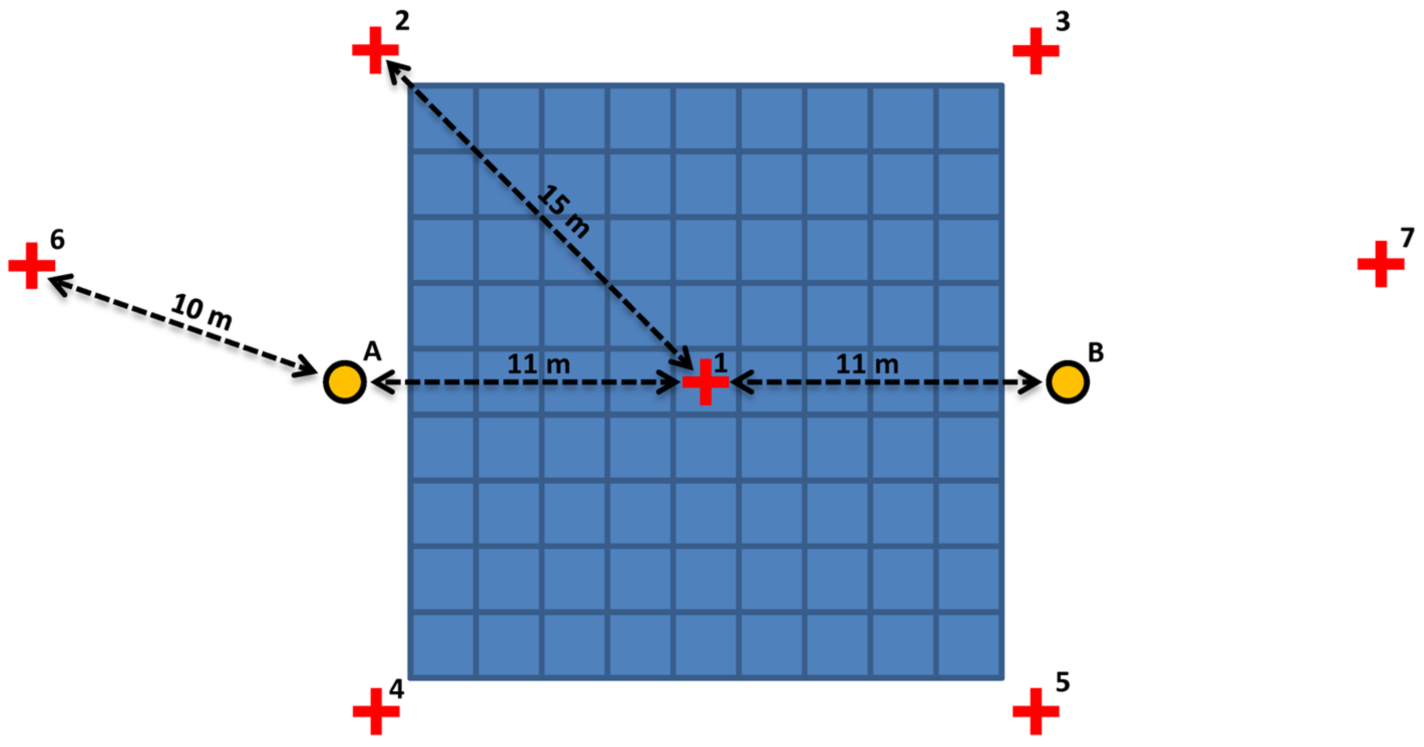
• Surface or control patch: the area of interest is the blue squared area, whose sides approximately follow a north–south and east–west orientation.
• Scan locations: The orange circles mark the locations A and B where the telescopic pole will be located. These two positions will follow roughly an east–west (or north–south) direction and will be about 11 m from the center of the patch (and, therefore, 22 m from each other). The 11 m are given by the 9 m from the patch center to its perimeter, plus 2 m to avoid the equipment being positioned directly over the patch.
• Georeferencing targets: The red crosses mark the position of a set of targets. The target coordinates will be obtained by GNSS observations and, therefore, used to georeference the scans. As can be seen in Figure 3, location A is surrounded by four targets (1, 2, 4 and 6) at a distance of about 10 m, and the same for location B (targets, 1, 3, 5 and 7). It can also be observed that both the patch area and the scanner stations are contained inside the convex hull of the targets, which is convenient in any coordinate transformation operation.

Table 2. Data collection workflow.

Step	Description
1	Patch center staking out. Given that the coordinates of the center of the patch are known, the GNSS equipment will be used to stake out this location on the ground. Since centimeter accuracy would not be required, the use of a mobile phone with its integrated GNSS sensor would be enough. Place a target at the staked-out location. This will be target #1.
2	Scan locations A and B staking out. An east–west (or north–south) alignment passing through target #1 will be marked. The orientation can be approximate, so any resource can be used (compass, mapping orientation, etc.). The scan locations A and B will be placed in this straight alignment, on each side of target #1 and 11 m far from it. Any signal can be used to mark A and B.
3	Targets distribution on the patch. The remaining six targets will be distributed around the patch, as indicated in Figure 3. Targets #2, #3, #4 and #5 will be located near the patch corners, approximately 15 m from target #1. Targets #6 and #7 would be furthest from the patch center, close to the established east–west alignment and about 10 m from the closest scan location (A or B).
4	Picture from the patch. The picture should include the whole patch and the targets should be visible.
5	Target measuring with GNSS equipment. Each target center will be measured with the GNSS equipment, checking that the horizontal and vertical standard uncertainty is below 3 cm. RTK will be the main method, using differential corrections by NTRIP. Each target will be named according to the pre-established code system (based on the patch identifier and the target numbering proposed in Figure 3).
6	Scanning from scan location A. All the PC capture system (tripod, telescopic pole, eccentric support and scanner) will be mounted over scan location A. The scanner must be in an inverted position to capture the ground data. The eccentric support will be rotated facing north (perpendicular to the straight alignment between scan locations A and B) and the scan will be performed. It should previously be ensured that the pole is vertical (using the hand level). Rotate the eccentric support 180° (facing south) and perform a second scan. A picture of the entire equipment (mast and laser scanner) will be taken during each scan, in which all or several targets will also appear.
7	Scanning from location B. Step 6 will be repeated, but this time from scan location B.
8	Final checking. The data storage device (e.g., ipad) will be checked on to ensure that the scans have been stored correctly. Otherwise, the necessary part of the work will be repeated.

contains the workflow to capture data for every patch.

2.2. Post-Processing Phase of Collected Data

After performing the data collection procedure as explained in Table 2, four independent PCs were available, each one relative to the scan’s origin point. The end goal of the following post-processing phase was to obtain a single PC in a specific coordinate system (CRS), which constitutes the reference patch (PAref) which allows us to assess its homologous patch in the same CRS derived from the LiDAR flight (PApro). Several steps are required (Figure 4):

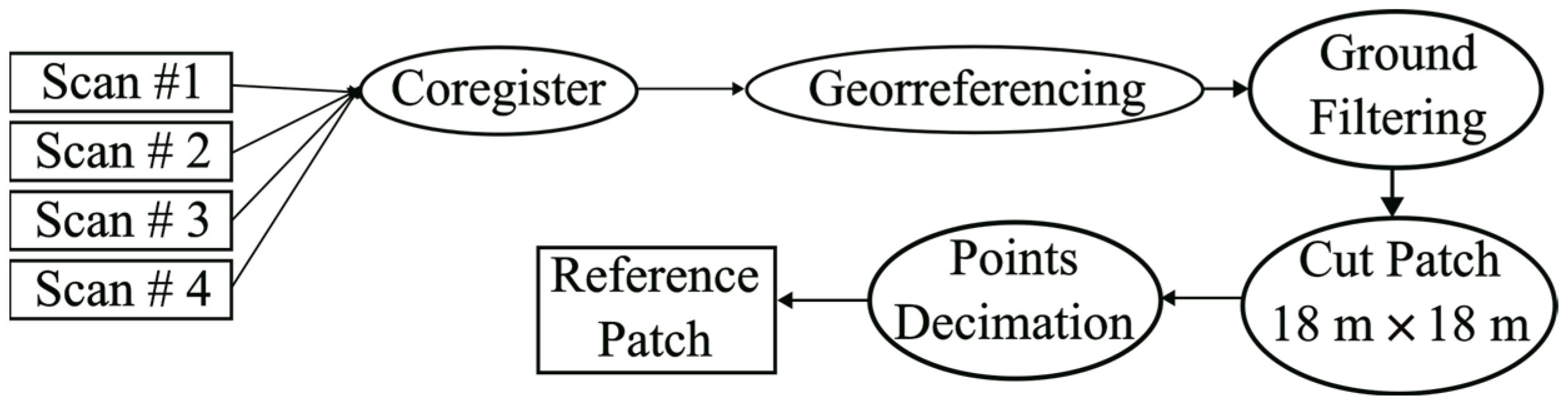
• PCs registration: The PCs are to be aligned one to another by finding a transformation that minimizes the difference between them. A single PC is obtained from this first step.
• PC georeferencing: The set of targets referred to in Table 2 are included in the PC, but also surveyed with GNSS in a specified CRS (e.g., ETRS89 and ellipsoidal height). Therefore, the center of the targets represents a set of ground control points (GCPs) which allow us to perform a coordinate transformation. The PC is to be transformed to the specified CRS. After steps 1 and 2, we obtain a registered georeferenced point cloud (RGPC).
• PC weeding: Ground filtering, clipping and decimation. The PC usually includes points that do not belong to the ground (fences, bushes, trees, people, cars, tripod, etc.). Also it includes points that are outside the limits of the patch of 18 m × 18 m. The density of points could also be much higher than required, especially if a DEM is to be obtained from the PC by interpolation. In consequence, the PC is to be (a) ground filtered, (b) clipped to the patch size and (c) decimated as required (e.g., applying a criterion based on the mean separation between points). After step 3, we obtained the PAref.

Furthermore, if a reference DEM is required (DEMref), for example, to assess any other product in a DEM format (DEMpro), another step is required:

4.

DEM interpolation from the PC: a DEM is obtained from PAref by interpolation, e.g., after a Voronoi triangulation over the PC.

2.3. Positional Accuracy of the RGPC

The positional accuracy of the PC should be checked to assure that it satisfies the requirements of the application. Nevertheless, the uncertainty of the individual points cannot be determined through repeated redundant measurements [14]. This is what would be called a Type A evaluation of uncertainty [15], based on a statistical analysis of a series of observations. Instead, the uncertainty can be calculated using the general law of error propagation from Type B evaluations [15] (manufacturer’s specifications, handbooks, personal experiences, etc.).

The registration and georeferencing processes are always performed with a software package, which offers different parameters to check the quality of the results. These result values should be aligned with an estimation of the sources of measurement uncertainty. Therefore, we propose to identify these sources and relate them with the results offered by the software.

First, it is important to take into account some considerations:

• The scanner is stable while measuring; therefore, the vibration of the measurement equipment is not a source of uncertainty.
• The scanner’s exact location is arbitrary and, therefore, there is no uncertainty in its position.
• The scanner does not require to be leveled, so there is no uncertainty in its inclination. Also, centering uncertainty [16] does not apply.

We will distinguish below between the local positional uncertainty of a point of the PC and its absolute positional uncertainty. The first is dependent on the scanner measurement quality, while the second depends both on the scanner and on the GNSS measurement quality.

2.3.1. Local Positional Uncertainty of a Point of the PC

Each point of each of the four PCs of a patch has a positional uncertainty relative to the origin of the coordinate system of the TLS, i.e., its local reference system. Its value can be estimated from the manufacturer information. Leica states in the specifications document of BLK 360 that the parameter one sigma (1σ) “3D point accuracy” is 0.006 m at a 10 m range and 0.008 m at a 20 m range [17]. Given that the patch size is 18 m × 18 m, a scanning spherical standard deviation (SSSD) of 0.008 can be assumed for any point (i.e., a standard deviation of 0.008 m in any direction).

When two PCs are aligned with one another in a registration process, a value for the difference between them is computed by the software. This value depends directly on the SSSD, for which the value is considered as equal for both PCs.

2.3.2. Absolute Positional Uncertainty (APU) of a Point of the RGPC

PCs are usually captured in a local coordinate system and then transformed to a CRS using GCPs by means of an indirect georeferencing procedure. No information regarding the position of the scanner is required, but at least three non-collinear GCPs are needed. The transformation is performed using the Helmert transformation, which does not introduce any distortions in the PC [14].

Applying the law of propagation of uncertainty, the uncertainty of the absolute coordinates of a point of the RGPC depends (1) on the uncertainty of the local coordinates of the point before the transformation (estimated with the SSSD value at a 20 m range) and (2) on the uncertainty of the transformation parameters, which in turn depends on the uncertainty of the local and absolute coordinates of the GCPs:

• The local coordinates of the GCPs are known from the PC and their uncertainty estimated through the value of the SSSD commented above (0.006 m at 10 m range).
• The absolute coordinates of the GCPs are obtained from a GNSS real-time kinematic (RTK) measurement. The quality of the data capture is usually known during the measurement, which can be considered a GNSS spherical standard deviation (GSSD) (0.03 m in our case, as will be mentioned in the following section). But the inclination of the hand-held rod-mounted GNSS antenna also influences the horizontal quality, with a rod standard deviation (RSD) which can be estimated at 0.005 m if a circular level is used and the antenna height is 2 m (in [18], it is estimated at 0.003 m for a height of 1.3 m). Furthermore, it must be considered that the center of each target will be identified as the closest point to the target center from the point cloud. This is another source of uncertainty, which can be called target center estimation (TCE), and is dependent on the density of the PC at 10 m. Considering a density of 0.01 m, the TCE could be estimated as 1/2 of the density, that is, 0.005 m.

A simple way to integrate all these sources of uncertainty in order to obtain the APU value is to compute the squared root of the sum of the squares as $APU=\sqrt{{SSSD}_{20}^2+{{TCE}^2+SSSD}_{10}^2+{GSSD}^2+{RSD}^2}$. With the referred values for each of these sources, a final value of $APU=\sqrt{\left({0.008}^2+{{0.005}^2+0.006}^2+{0.030}^2+{0.005}^2\right)}=0.032 \mathrm{m}$ is obtained. This value represents the radius of an uncertainty sphere and, therefore, also the uncertainty value in any direction, horizontal or vertical. Actually, the RSD does not affect the vertical direction, but its influence in the APU value is negligible. The APU value depends mainly on the GSSD value.

Table 3. Terms used for estimation of the absolute positional uncertainty (APU) of a point of the PC in the desired CRS.

Name	Abbreviature	Description and Quantification
Scanning spherical standard deviation at 20 m	SSSD20	Measurement uncertainty from manufacturer′s specification, 0.008 m in the case of Leica BLK 360.
Target center estimation	TCE	Half the density of points when scanning targets, 1/2 × 0.01 m in our scanning configuration.
Scanning spherical standard deviation at 10 m	SSSD10	Measurement uncertainty from manufacturer’s specification, 0.006 m in the case of Leica BLK 360.
GNSS spherical standard deviation	GSSD	Measurement uncertainty offered by the GNSS equipment in RTK. 0.03 m in our RTK measurement.
Rod standard deviation	RSD	Inclination of the hand-held rod-mounted GNSS antenna. Estimated at 0.005 m.

summarizes the sources of all of the terms introduced in this section.

2.4. Methodology for the Patch-Based Accuracy Control of a DEM

As stated in Section 1, there are many different point-based PAAMs. For clarity, it is good practice to present them in a comparable form. In [8], four standards are summarized, each one in a table with a focus on the comparison method, the positional component (s) (e.g., X, Y and Z) on which the calculation can be performed, the existence of a standard value, a brief description of the method, the full procedure and a reference to the original source. Here, we propose to follow the same structure to summarize the new proposed methodology for DEM products.

The framework in which the methodology is proposed is the following: a DEMref is available for every measured patch after the data collection and post-processing phase. As occurs with the point-based PAAMs, different patch-based PAAMS could be proposed for the same data, each one with a different level of complexity, or emphasizing some aspect, etc. In

Table 4. Methodology for a patch-based accuracy control of DEMs.

Comparison Method	With Sources Having Higher Accuracy.
Positional component	Vertical.
Element type	Patches. Each patch is given by a DEM.
Accuracy standard	A result is provided, and the user has to consider whether or not it is fit for purpose. It is expressed by the range from 5- to 95-percentile (a 90% percentile range centered on the median value).
Description	The product is compared to a reference with higher accuracy. The vertical component of the product is assessed. A sample of at least 30 well-distributed patches is used. Accuracy is evaluated through the observed distribution function from the elevation differences between the product and the reference. It allows us to avoid evaluating accuracy through parameters. This situation is preferred for DEMs since it is known that the error does not always follow a parametric distribution, like the normal distribution.
Procedure	It is given that a sample of n (n ≥ 30) reference patches (DEMref) is available and: They are randomly spatially distributed; The range of elevations of DEMpro is covered; A set of polygons defining their limits is available. Crop the product (DEMpro) to match the set of polygons. For every point from the cropped DEMpro, interpolate the elevation in DEMref at the same location. For every point from the cropped product, calculate the elevation error:
	$e_{Z_i}=z_{p_i}-z_{r_i}$
	where: $z_{p_i}$ is the elevation in the product. $z_{r_i}$ is the interpolated elevation in the reference. 4. Compute the 2.5% percentile (p2.5) and the 97.5% percentile (p97.5) from all eZi values. 5. Define and publish the 95% percentile range interval (r95) from 2.5- to 97.5-percentile:
	$r_{95} = [p_{2.5}, p_{97.5}]$

we present a simple proposal for better understanding, in which accuracy is evaluated through a percentile interval of the observed distribution function from the elevation differences between the product and the reference. An advantage of the proposed method is its simplicity regarding calculations. As a disadvantage, it does not provide much insight into the statistical behavior of errors (e.g., bias and deviation for the normal case).

But any other proposal could be developed depending on the needs of the study in question. As an example, the evaluation of a DEM surface through patches allows the evaluation to be carried out on the presence of terrain features (e.g., streams, small hills, small rock masses, etc.), or on the analysis of the distribution of slopes and aspects, etc. Thus, with this new perspective, the analysis possibilities are greater and more applied.

3. Practical Case

Started in 2009, the project PNOA-LiDAR from the national mapping agency in Spain (Instituto Geográfico Nacional) is capturing three-dimensional information using airborne LiDAR sensors throughout the entire territory, generating a series of products from this capture, such as point clouds, DEMs, DSMs, etc. The density of capture has evolved from 0.5 points/m² (first coverture, between 2009 and 2015) to 5 points/m² (third coverture, between 2002 and 2025). But in 2017, an experimental LiDAR flight was carried out in the Foral Community of Navarra (Spain) using Single-Photon LiDAR technology with the Leica SPL100 sensor (more info about this data capture in [19]), increasing the density of capture to 14 points/m². We propose to assess the accuracy of these data.

A set of 30 patches distributed throughout the study area were measured following the data collection procedure explained in Section 2.1. It is important to remember that the ASPRS [3] recommends to assess the LiDAR performance in an open terrain where there is no vegetation to disturb its performance, mainly in open (bare soil, sand, gravel and short grass) and urban (asphalt and concrete) terrain surfaces. The real time positioning service of Navarra (RGAN, Red de Geodesia Activa de Navarra), available online [https://www.navarra.es/es/web/rgan (accessed on 27 November 2024), was used for the GNSS RTK measurement.

Section 3.1 details the software quality results for one of the 30 PArefs, relating them to Section 2.3. Section 3.2 clarifies details about deriving a high-density DEFref from each PAref. Finally, Section 3.3 gives an example of a positional quality analysis. This uses the whole sample of 30 patches and is, therefore, different from the traditional analysis based on a set of control points.

3.1. Software Quality Results

For the post-processing phase of the collected data, Leica’s Cyclone Register 360 software was used.

Table 5. Summary of the report of Cyclone Register 360 to obtain an RGPC of a PAref.

Parameter	Value	Description
Number of scans	4	Number of PCs that have been measured
Number of links	6	Number of pairs from the number of PCs
Overall cloud-to-cloud error	0.008 m	Mean error from the registration process
Cloud-to-cloud error: Link 1 Link 2 Link 3 Link 4 Link 5 Link 6	0.008 m 0.013 m 0.009 m 0.003 m 0.009 m 0.021 m	Mean error between each pair of PCs from the registration process
Mean georeferencing error	0.021 m	Mean error in each target after registration and georeferencing
Error in each target: Target 1 Target 2 Target 3 Target 4 Target 5 Target 6 Target 7	0.031 m 0.038 m 0.007 m 0.013 m 0.023 m 0.004 m 0.012 m	Mean error in each target after registration and georeferencing

summarizes the different parameters included in the report of this software to obtain an RGPC. The main aspects to highlight are

• A registration overall error of 0.008 m is obtained. The error between each possible pair of PCs, labeled by a link number, is also included, with values ranging from 0.003 m to 0.021 m. These results are consistent with the local positional uncertainty commented on in Section 2.3, which was represented by the parameter SSSD₂₀ from the manufacturer. Considering this parameter as equal for each PC, with a value of 0.008 m, the value of the difference between two PCs can be assumed to be SSSD₂₀ × 2^1/2 = 0.011 m. Only link six seems to be higher than expected.
• A mean georeferencing error of 0.021 m is obtained. The error for each target is also included, with values ranging between 0.004 m and 0.038 m. These results are consistent with the APU value from Section 2.3.

3.2. Deriving DEMref from the RGPC

As mentioned in Section 2.2, the density of points could be much higher than required. Given that the TLS was configured for a density of 0.01 m and that the RGPC is a result of the registration of four PCs over the same patch, the density of the RGPC could be much more than one point in a cm². This is an excessive number of points and, therefore, the RGPC must be decimated before deriving the DEMref. In order to maintain a high-density DEMref, which could be used to assess the quality of a high-density product in a DEM format (DEMpro), this decimation is configured to reduce the number of points until the mean separation between the points is 0.01 m. At the same time, this weeding process includes ground filtering and clipping to the patch size of 18 m × 18 m. A PAref is then obtained. After a Voronoi triangulation over this PAref, a DEMref with a 0.01 m resolution (cell size 1 cm, density 10,000 points/m²) is obtained by interpolation, which finally may be used to assess any DEMpro. As [20] demonstrates, assuming that all the vertices of the triangle have the same uncertainty, the average uncertainty in an interpolation inside the triangle is one-half of the uncertainty of the vertices. This indicates that, in this case, the result is not degraded from this point of view.

3.3. Example of Positional Accuracy Analysis Using the Sample of Patches (DEMref)

As indicated in Section 1, our patch strategy for obtaining a high-density DEM (DEMref) allows us to assess airborne LiDAR data and the derived DEM (DEMpro) by applying analysis methods different from the traditional ones based on a set of control points. Now two surfaces, DEMref and DEMpro, represent the same reality. If the first has a greater density and accuracy (at least three times better [21]) than the second, it could be suitable for a positional accuracy assessment. This requirement is satisfied since the specifications of the experimental LiDAR flight indicate an absolute horizontal standard deviation of 0.2 m, an absolute vertical standard deviation of 0.15 m and a density of 14 points/m².

An important aspect of this new perspective is that it allows us to move from evaluating accuracy through parameters (e.g., RMSE, standard deviation, etc.) to analyzing accuracy through the differences between the observed distribution functions. This situation is much more suitable for DEMs since it is known that the error does not always follow a parametric distribution, like the Normal distribution. In Section 2.4, a methodology for a patch-based accuracy control of DEMs is summarized, which ends with a result, given by the 2.5- to 97.5-percentile interval of the observed distribution function from the elevation differences between DEMref and DEMpro. Nevertheless, in this section, we will offer a wider exploration of the results, aiming to show the possibilities of this new perspective. In Section 3.3.1, a comparison between the density distribution functions for the elevation is presented. In Section 3.3.2, the attention is centered on the discrepancies throughout the histogram, the normal probability plot and the distribution function.

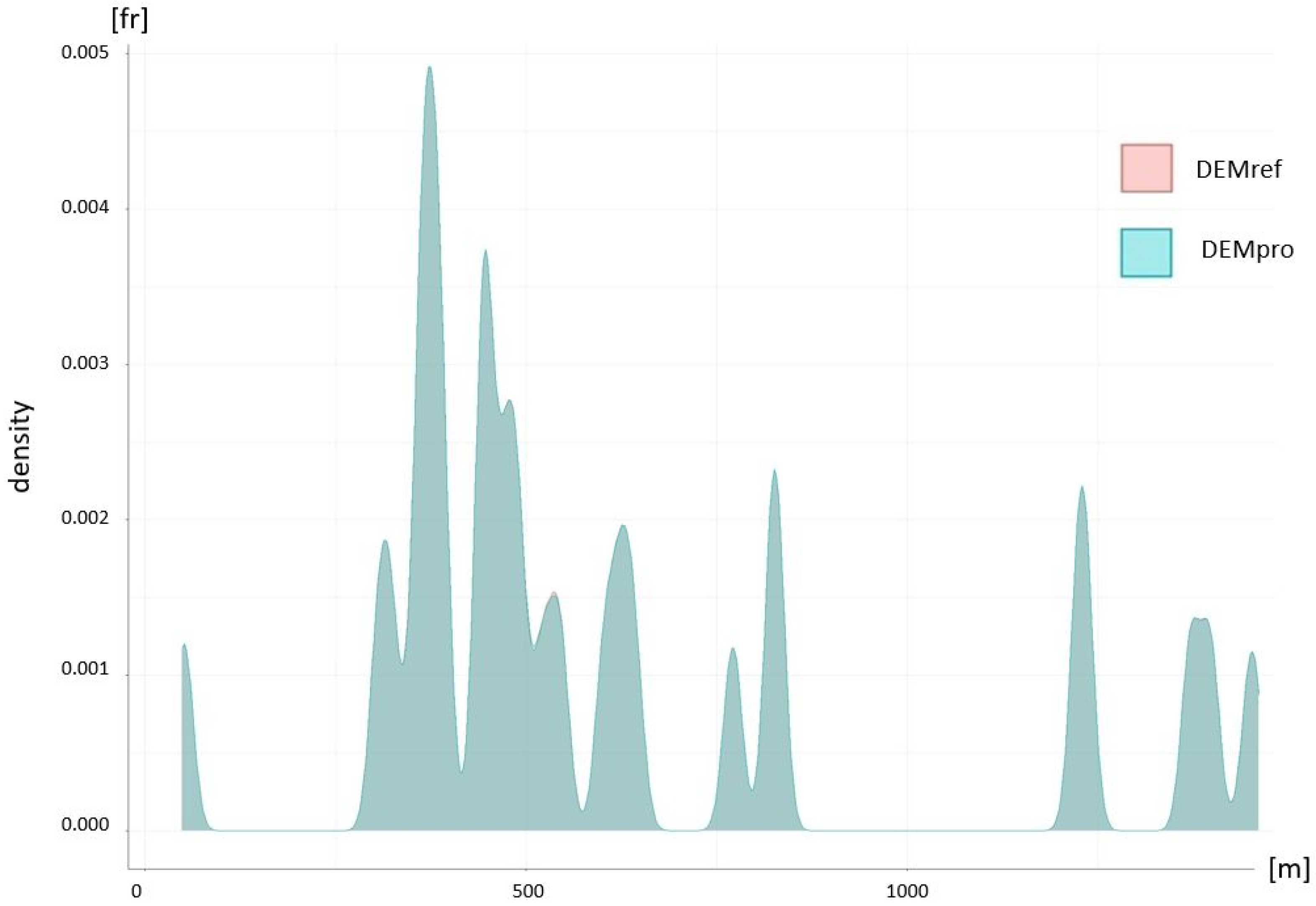
3.3.1. Analysis of the Elevation Distribution Functions of DEMref and DEMpro

Figure 5 presents the superposition of the density functions of the data that have been collected in the 30 patches that have been executed in this assessment. The product is represented in a bluish color and the reference in a pinkish color. This representation is interesting because it shows the following: On the one hand, there is a very high overlap between the two datasets (product and reference). In fact, the bluish color overlaps perfectly on the pinkish color. As a method for measuring the goodness of fit of the product data to the reference data, a calculation was carried out according to the method proposed by [22]. In this way, the overlap index takes the value 0.9978, very close to unity, which indicates a very similar behavior of both density functions. On the other hand, this representation shows numerous peaks that correspond to each of the patches. Figure shows 4 windows or intervals in which there are no data (density). Therefore, this representation allows us to analyze whether the sampling carried out covers the entire range of elevations present in the area of interest. In our case, the distribution is quite adequate, although there are two uncovered area: one at around 100 m of elevation and another at around 1000 m of elevation.

Figure 6 represents the cumulative probability function, that is, the integral of Figure 5 above. In this figure, you can also see the perfect superposition of the two curves and the presence of patches and uncovered areas. The patches contribute data to the distribution and correspond to the parts of the curves that rise, while the elevation intervals that are not covered by the sample correspond to the horizontal zones. Therefore, this way of working allows for a much more complete analysis of the representativeness of the sample than that allowed by point-based PAAMS.

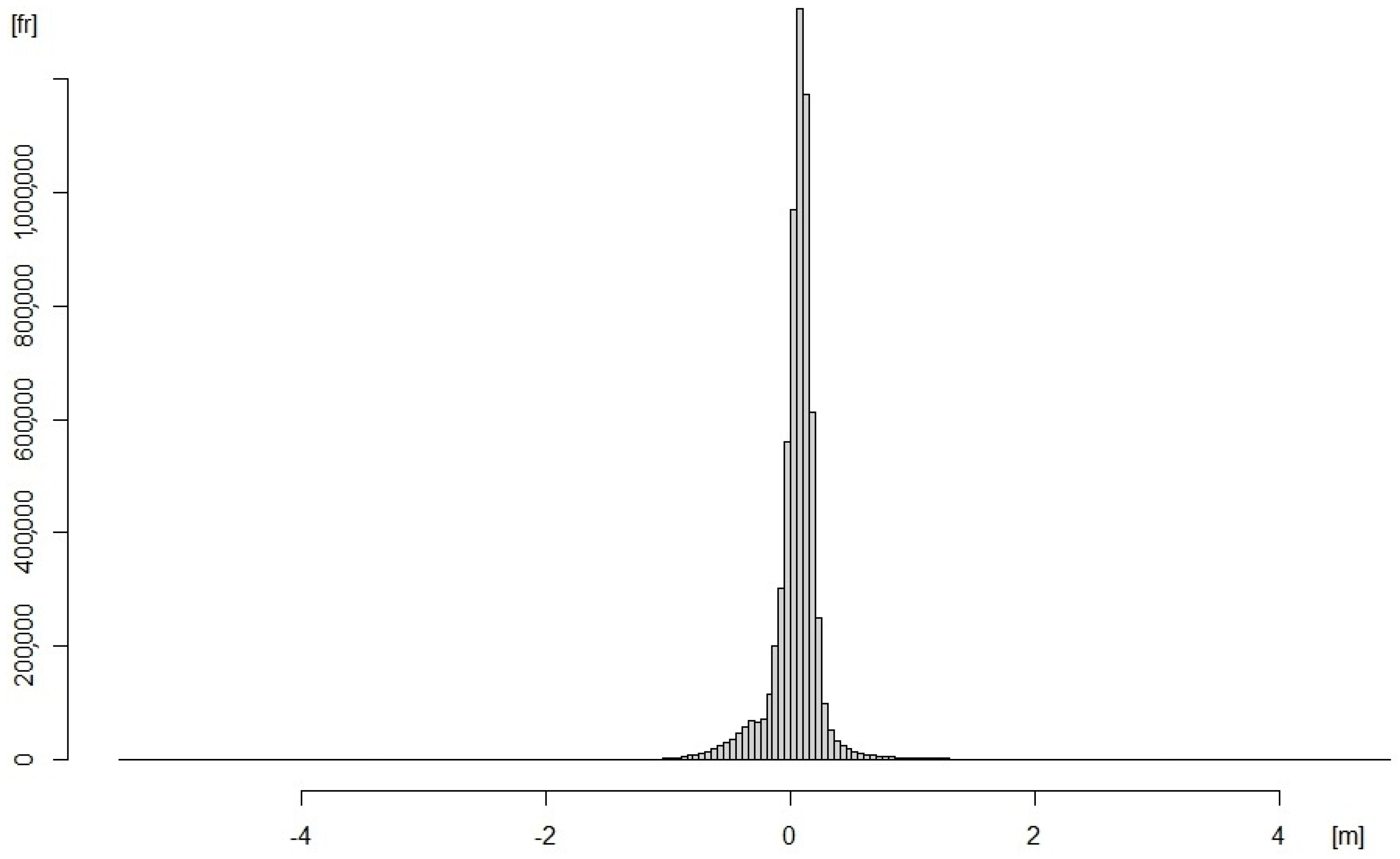
3.3.2. Analysis of the Discrepancies Between DEMref and DEMpro

Once the distribution of the elevations has been analyzed, we can proceed to analyze the discrepancies between the two datasets. Following the procedure presented in Table 4, a set of elevation errors, or discrepancies, is obtained from step 3. The next steps indicate to compute the 2.5% and 97.5% percentiles and define the 95%-range percentile interval: $r_{95}=[p_{2.5},p_{97.5}]$. Although it is not necessary to obtain this range, below we present some charts that could be obtained and a short interpretation:

• Obtaining the histogram (Figure 7) is recommended to begin the analysis. It can be seen that the curve does not present symmetry and that it does not follow the shape of the Gaussian bell as it is more pointed.
• The normal probability plot (Figure 8) is a special case of the Q–Q probability plot which compares the distribution of a sample to a theoretical standard normal distribution. It helps to confirm that the discrepancy data are not normal since the points in the chart would then lie close to a straight line.
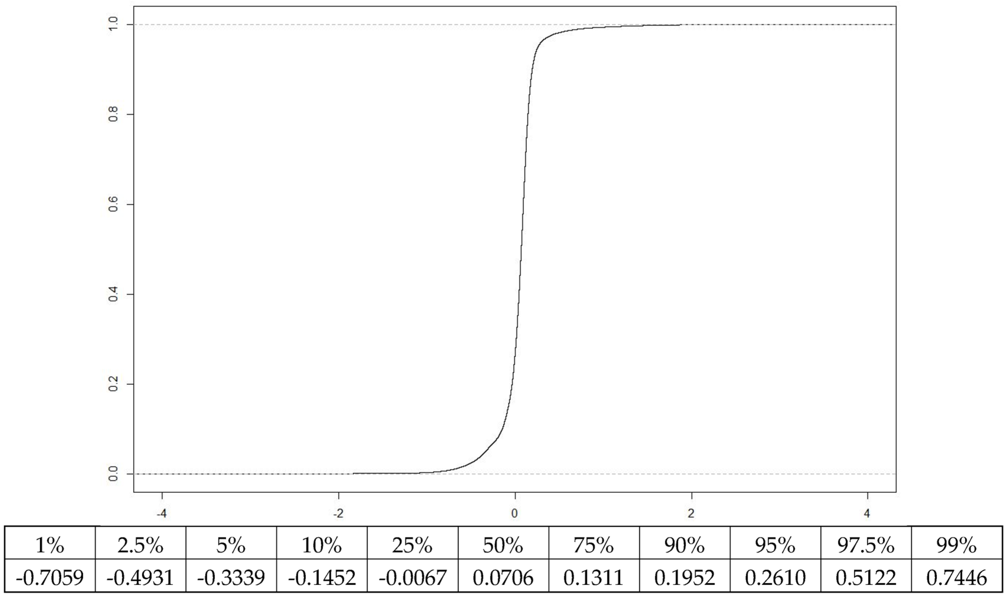
• The probability distribution (Figure 9) is accompanied by the percentiles presented at the bottom of the chart. Requested from the procedure in Table 4, 95 percent of the cases are in the interval $r_{95}=[-0.4932,0.5122]$. From another point of view, if we consider the interval given by the 50% percentile (0.0706 m) and the vertical uncertainty indicated for the experimental LiDAR flight (σ = ±0.15 m), we obtain the interval [−0.0794, 0.2206] m, for which the probability included is 0.7803. This value is somewhat greater than 0.682, which is the probability in the interval [−1σ, +1σ] in a normal distribution function with parameters mean = 0 and σ = 1. This implies that the observed data have a somewhat smaller dispersion than those from a normal distribution. Also, from the data, it can be deduced that there is a bias since the value corresponding to the 50% percentile is 0.0706 m.

3.4. Estimation of Costs for Field Data Collection

The mean time spent on a simple scan, including taking pictures, is 2 min and 40 s. However, what takes the most time, 30 min, is the setup of the point cloud capture system (tripod, telescopic pole, eccentric support and TLS) for every pair of scans. Since two setups are performed for each patch, capturing a patch requires approximately 1 h of field work. If a patch capture campaign is proposed over a wide area of territory, as may be the case for a Spanish region, and the patches are supposed to be evenly distributed, the patches capture rate could be estimated at five per day.

Assuming rentals of EUR 430/day, including the BLK360, tripod and telescopic pole, the patch cost would be EUR 86/patch, without considering the required conveyance or the cost of the human team (remuneration, maintenance and accommodation costs).

3.5. Comparison with a Point-Based PAAM

As stated in the introduction section, the point-based PAAMs are traditionally applied for a DEM positional accuracy assessments. A patch-based approach is not a substitute for those methods since the results and analysis are complementary.

Table 6. Main characteristics of point-based and patch-based PAAMs.

#	Item	Point-Based (Traditional Methods)	Patch-Based
1	Comparison method	With sources having higher accuracy	With sources having higher accuracy
2	Quality component	Vertical Accuracy	Vertical accuracy, surface derivates (slope, aspect, curvatures, flatness)
3	Element type	Isolated points	Point cloud
4	Required equipment	GNSS (1)	GNSS + TLS
5	Complementary equipment	Standard pole	Targets, long pole Special tripod, etc.
6	Cost of the equipment	Medium (several thousand EUR/USD)	High (several tens of thousands EUR/USD)
7	Minimum human team	1 operator (2)	2 operators
8	Applicable positional accuracy standards	EMAS, NSSDA, ASPRS, UNE 148,002, etc. (3)	Not available yet
9	Sample size	Minimum recommendation: 20 ground control points	Minimum recommendation: 20 ground control patches
10	Sampling scheme	Random	Random
11	Time required for the collection of a sample (4)	Short (a few minutes)	Medium (1 h)
12	Complexity of data analysis	Low, point-to-point discrepancies are calculated and quality measures (e.g., RMSE) are derived	Medium, the patch and the homologous surface must be available. Interpolations must be performed or work with TIN. The distribution function is generated
13	Information provided by the result for the case of estimation-based standards (5)	A parameter (e.g., RMSE, or standard deviation) under a normal probability distribution assumption. For example, meters for a given confidence level (e.g., 5 m at 95% confidence level) (see NSSDA).	Quantile (values corresponding to the desired percentile). The observed distribution function is available
14	Information provided by the result for the case of control-based standards (6)	An acceptance or rejection decision under a normal probability distribution assumption of the parameters	Acceptance or rejection based on the observed distribution function

(¹) Other surveying and geodetic instruments can be used. (²) A real-time GNSS positioning service is supposed to be available in the region. (³) In [8], a summary for different point-based positional accuracy standards can be found. (⁴) Travel is not considered, only the preparation of the instruments and data collection. (⁵) Estimate-based standards are those that provide the value of a parameter as accurately as possible. (⁶) Control-based standards are those that offer an acceptance or rejection decision within an established framework of producer and user risks (type I and II errors).

clarifies the similarities and differences between both type of PAAMs when using GNSS and TLS equipment. Both approaches need sources of data with higher accuracy (item #1), assess the vertical accuracy (#2), need a minimum sample size of 20 points/patches (#9) and need a random sampling scheme (#10). But the patch-based proposal allows us to assess surface derivatives (#2), offers a more complex data analysis (#12) with results based on the observed distribution function (#13, #14), not assuming a normal probability distribution. These advantages are not free since they imply more equipment with a higher cost (#4, #5 and #6), a bigger human team (#7) and more time required for the data collection (#11). Obviously, there are still no established positional accuracy standards for the patch-based approach, while in the point-based approach, they are fully stablished (#8).

As an example of applying a point-based PAAM to our practical case, the NSSDA [23] standard has been applied to a sample of 30 ground control points, each of them located in each of the 30 patches. The reference coordinates were measured with GNSS and the product coordinates were interpolated from the experimental LiDAR flight at the same location. The NSSDA is an estimation method based on the assumption of normality of the error data and it provides a positional accuracy index in real units in the field. Specifically, it uses the RMSE and presents it at a confidence level of 95%, assuming that the systematic errors have been eliminated as best as possible. The obtained results are presented in

Table 7. Results of the point-based PAAM application.

Measure	Value
RMSE	0.082 m
NSSDAz	0.160 m

, where NSSDA_z = 0.160 m, which means that only 5% of the population presents an error higher than 0.160 m. The declared specification is an absolute vertical standard deviation of 0.15 m; therefore, if only observing the NSSDA result, the experimental LiDAR flight can be assumed to be better than expected.

Nevertheless, the assumption of the absence of systematic errors is questionable, as can be deduced from Figure 10, where the presence of a positive bias in the elevation discrepancy is noted. Also the assumption of normality should be checked.

4. Conclusions

The present paper explains a method for obtaining field patches, or control surfaces, for positional accuracy assessments, specifically on airborne LiDAR data and derived DEMs. The goal is to use patches instead of control points to assess the DEMs’ quality since patches have the same surface nature as DEMs. This patch-based PAAM aims to measure a set of high-density and high-quality georeferenced ground point clouds, each one constituting a PAref with a derived DEMref. PAref and DEMref allow for assessing the quality of a PApro or a derived DEMpro. Using patches overcomes the limitation of having “well-defined and easily identifiable points”, which is an essential requirement for evaluating the positional accuracy. This limitation is circumvented, but as a consequence of the superficial nature of the control elements, the analysis method must also be different, for example, computing a goodness-of-fit test between the elevation distributions of the product and the reference objects, etc.

An example has been materialized for the case of a single 18 m × 18 m size patch to assess the data from an experimental LiDAR flight in Navarra (Spain). To obtain the PAref, a Leica BLK360 TLS, stationed at a 7 m height in an inverted position on a telescopic pole, was used. After the described processing of the PC, the PAref had a suitable density and accuracy (at least three times higher) for the assessment of its homologous PApro from the experimental LiDAR flight, whose density was 14 points/m² and horizontal and vertical standard deviation were 0.20 m and 0.15 m, respectively.

As a final conclusion, the proposed method has the advantage of being able to assess a DEM at practically any resolution, given the high density of points obtained with the TLS in the PAref survey and provided that the absolute positional uncertainty of the PAref is below 0.05 m.

The example of the positional accuracy analysis developed has been based on the distribution functions of the data, and not on the determination of classic parameters such as the RMSE or the mean value and deviation of the sample. This approach is more powerful and frees the data from the need to follow a predetermined statistical model (e.g., the Gaussian model). Anyway, it should be noted that patch-based PAAMs are not a substitute for point-based PAAMs since the results are not comparable. The analysis capacity of the former is complementary to that of the latter.

On the other hand, although the example developed has been presented for an open-field environment, with slight adaptations, it can be applied in urban environments. In this case, we could work together with inverted and non-inverted surveys with the aim of adequately covering horizontal (e.g., sidewalks, pavements, etc.) and vertical surfaces (e.g., building facades). In a near future, it is our interest to advance in this field of application in order to offer a rigorous method that allows controlling the point clouds that are incorporated into the digital twins of our cities.

References

1. ISO 19157-1:2023; Geographic Information—Data Quality—Part 1: General Requirements. International Organization for Standardization: Geneva, Switzerland, 2023.
2. Bühler, Y.; Marty, M.; Ginzler, C. High Resolution DEM Generation in High-Alpine Terrain Using Airborne Remote Sensing Techniques. Trans. GIS 2012, 16, 635–647. [Google Scholar] [CrossRef]
3. ASPRS. ASPRS Positional Accuracy Standards for Digital Geospatial Data, 2nd ed.; American Society for Photogrammetry and Remote Sensing: Baton Rouge, LA, USA, 2023. [Google Scholar]
4. Zandbergen, P.A. Positional Accuracy of Spatial Data: Non-Normal Distributions and a Critique of the National Standard for Spatial Data Accuracy. Trans. GIS 2008, 12, 103–130. [Google Scholar] [CrossRef]
5. Maune, D.F.; Nayegandhi, A. (Eds.) Digital Elevation Model Technologies and Applications: The DEM Users Manual, 3rd ed.; ASPRS: Baton Rouge, LA, USA, 2019. [Google Scholar]
6. Ariza López, F.J.; Atkinson Gordo, A.D. Analysis of Some Positional Accuracy Assessment Methodologies. J. Surv. Eng. 2008, 134, 45–54. [Google Scholar] [CrossRef]
7. Mesa-Mingorance, J.L.; Ariza-López, F.J. Accuracy Assessment of Digital Elevation Models (DEMs): A Critical Review of Practices of the Past Three Decades. Remote Sens. 2020, 12, 2630. [Google Scholar] [CrossRef]
8. Ariza-López, F.J.; García-Balboa, J.L.; Rodríguez-Avi, J.; Robledo-Ceballos, J. Guide for the Positional Accuracy Assessment of GEOSPATIAL Data; Occasional Publications #563; Pan American Institute of Geography and History: Mexico City, Mexico, 2021. [Google Scholar]
9. Ariza-López, F.J.; Rodríguez-Avi, J.; Reinoso-Gordo, J.F.; Mozas-Calvache, A.T.; Ruiz-Lendínez, J.J.; García-Balboa, J.L. Evaluación de MDE por medio de parches de control. In Proceedings of the XIX Congreso de Tecnologías de la Información Geográfica, Zaragoza, Spain, 12–14 September 2022; TIG al servicio de los, ODS. de la Riva-Fernández, J., Lamelas-Gracias, M.T., Montorio-Llovería, R., Pérez-Cabello, F., Rodrigues-Mimbrero, M., Eds.; Servicio de Publicaciones Universidad de Zaragoza: Zaragoza, Spain, 2022. [Google Scholar]
10. Kim, M.; Park, S.; Danielson, J.; Irwin, J.; Stensaas, G.; Stoker, J.; Nimetz, J. General External Uncertainty Models of Three-Plane Intersection Point for 3D Absolute Accuracy Assessment of Lidar Point Cloud. Remote Sens. 2019, 11, 2737. [Google Scholar] [CrossRef]
11. Brown, R.; Hartzell, P.; Glennie, C. Evaluation of SPL100 Single Photon Lidar Data. Remote Sens. 2020, 12, 722. [Google Scholar] [CrossRef]
12. Zandbergen, P.A. Characterizing the error distribution of lidar elevation data for North Carolina. Int. J. Remote Sens. 2011, 32, 409–430. [Google Scholar] [CrossRef]
13. Ariza-López, F.J.; Rodríguez-Avi, J.; González-Aguilera, D.; Rodríguez-Gonzálvez, P. A New Method for Positional Accuracy Control for Non-Normal Errors Applied to Airborne Laser Scanner Data. Appl. Sci. 2019, 9, 3887. [Google Scholar] [CrossRef]
14. Uggla, G.; Horemuz, M. Conceptualizing Georeferencing for Terrestrial Laser Scanning and Improving Point Cloud Metadata. J. Surv. Eng. 2021, 147, 02520001. [Google Scholar] [CrossRef]
15. JCGM 100:2008; OIML Evaluation of Measurement Data—Guide to the Expression of Uncertainty in Measurement. Joint Committee for Guides in Metrology: Paris, France, 2008.
16. García-Balboa, J.L.; Ruiz-Armenteros, A.M.; Rodríguez-Avi, J.; Reinoso-Gordo, J.F.; Robledillo-Román, J. A Field Procedure for the Assessment of the Centring Uncertainty of Geodetic and Surveying Instruments. Sensors 2018, 18, 3187. [Google Scholar] [CrossRef] [PubMed]
17. Leica Geosystems AG. Leica BLK360 User Manual Version 2.0 English; Leica Geosystems AG: Heinrich-Wild-Strasse, Heerbrugg, Switzerland, 2017. [Google Scholar]
18. Ruiz-Armenteros, A.M.; García-Balboa, J.L.; Mesa-Mingorance, J.L.; Ruiz-Lendínez, J.J.; Ramos-Galán, M.I. Contribution of instrument centring to the uncertainty of a horizontal angle. Surv. Rev. 2013, 45, 305–314. [Google Scholar] [CrossRef]
19. Mandlburger, G.; Jutzi, B. On the Feasibility of Water Surface Mapping with Single Photon LiDAR. ISPRS Int. J. Geo-Inf. 2019, 8, 188. [Google Scholar] [CrossRef]
20. Shi, W. Principles of Modeling Uncertainties in Spatial Data and Spatial Analyses; CRC Press: Boca Raton, FL, USA, 2009; ISBN 978-0-429-14952-8. [Google Scholar]
21. ASPRS. ASPRS Positional Accuracy Standards for Digital Geospatial Data. Photogramm. Eng. Remote Sens. 2015, 81, A1–A26. [Google Scholar] [CrossRef]
22. Pastore, M.; Calcagnì, A. Measuring Distribution Similarities Between Samples: A Distribution-Free Overlapping Index. Front. Psychol. 2019, 10, 01089. [Google Scholar] [CrossRef] [PubMed]
23. FGDC. Geospatial Positioning Accuracy Standards, Part 3: National Standard for Spatial Data Accuracy; FGDC-STD-007.3-1998; Federal Geographic Data Committee: Reston, VA, USA, 1998.
Figure 1. Angle of incidence of the laser on the ground at a standard height of the TLS of 1.5 m and when the TLS is raised up to 7 m high in inverted position, for a horizontal distance of 15 m.
Remotesensing 16 04516 g001
Figure 2. Point cloud capture system: tripod, telescopic pole, eccentric support and scanner in inverted position: (a) on a conventional tripod, (b) on a high tripod.
Remotesensing 16 04516 g002
Figure 3. Sketch of the scanner stations (orange circles A and B) and targets (red crosses 1–7) distribution required to obtain an 18 m × 18 m patch.
Remotesensing 16 04516 g003
Figure 4. Workflow followed to produce the PAref from the scans.
Remotesensing 16 04516 g004
Figure 5. Overlayed density distribution functions for the elevations of all the patches (DEMref in pinkish, DEMpro in bluish). DEMpro overlaps perfectly on DEMref (therefore, pinkish is not appreciated).
Remotesensing 16 04516 g005
Figure 6. Overlayed probability distribution functions for the elevations of all the patches (DEMref in red, DEMpro in blue). DEMpro overlaps perfectly on DEMref. The elevation range is on the horizontal axis and the accumulated relative frequency is presented on the vertical axis.
Remotesensing 16 04516 g006
Figure 7. Histogram of the error distribution between DEMref and DEMpro for all the patches. The elevation discrepancy range is on the horizontal axis and the absolute frequency is presented on the vertical axis. It can be seen that this distribution is not symmetrical and that its shape is more pointed than that of a Gaussian distribution.
Remotesensing 16 04516 g007
Figure 8. Normal probability plot of the elevation discrepancies between DEMref and DEMpro. The population quantiles are on the horizontal axis and the sample quantiles are on the vertical axis. Data are represented by means or points (circles), which are not close to a straight line and therefore do not follow a normal distribution. As a reference, the thin line passes through the first and third quartiles.
Remotesensing 16 04516 g008
Figure 9. Distribution function of the discrepancies of elevations between DEMref and DEMpro for all the patches. The elevation discrepancy is on the horizontal axis and the relative frequency is presented on the vertical axis. Some percentile values are included at the bottom of the chart. Horizontal dashed lines are included as a reference for probabilities with values 0.0 and 1.0.
Remotesensing 16 04516 g009
Figure 10. Overlayed cumulative relative frequency for the elevation discrepancy (in blue) versus cumulative relative frequency of a normal distribution (with the same mean and standard deviation as the elevation discrepancy sample) (in red).
Remotesensing 16 04516 g010