
Performance Assessment of Landsat-9 Atmospheric Correction Methods in Global Aquatic Systems

 ,
, 

Abstract
1. Introduction
2. Materials and Methods
2.1. Satellite Data
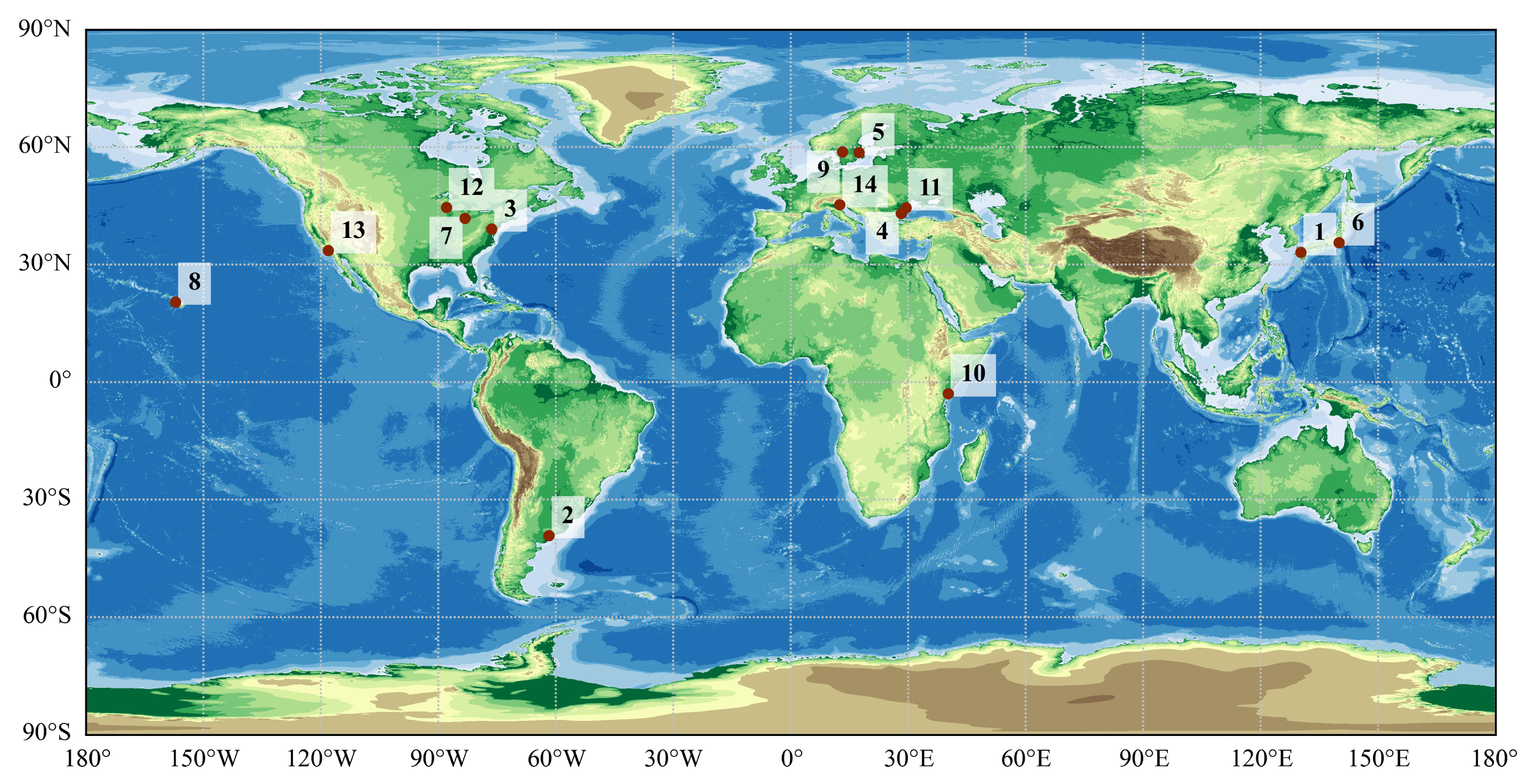
2.2. In-Situ Data
2.3. Atmospheric Correction Methods
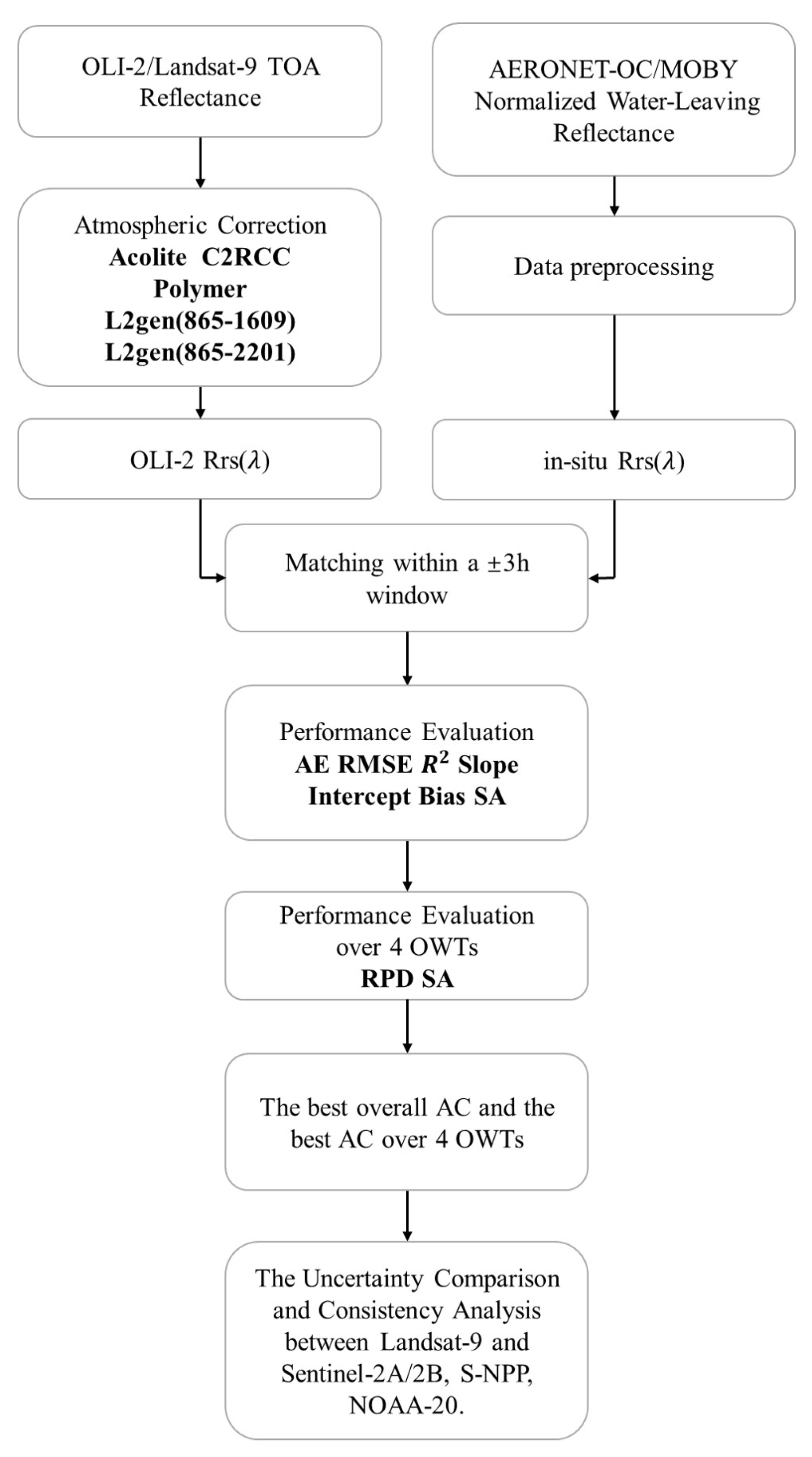
2.4. Procedure for Comparing Satellite and In-Situ Measurements
2.5. Evaluation Indicators
3. Results
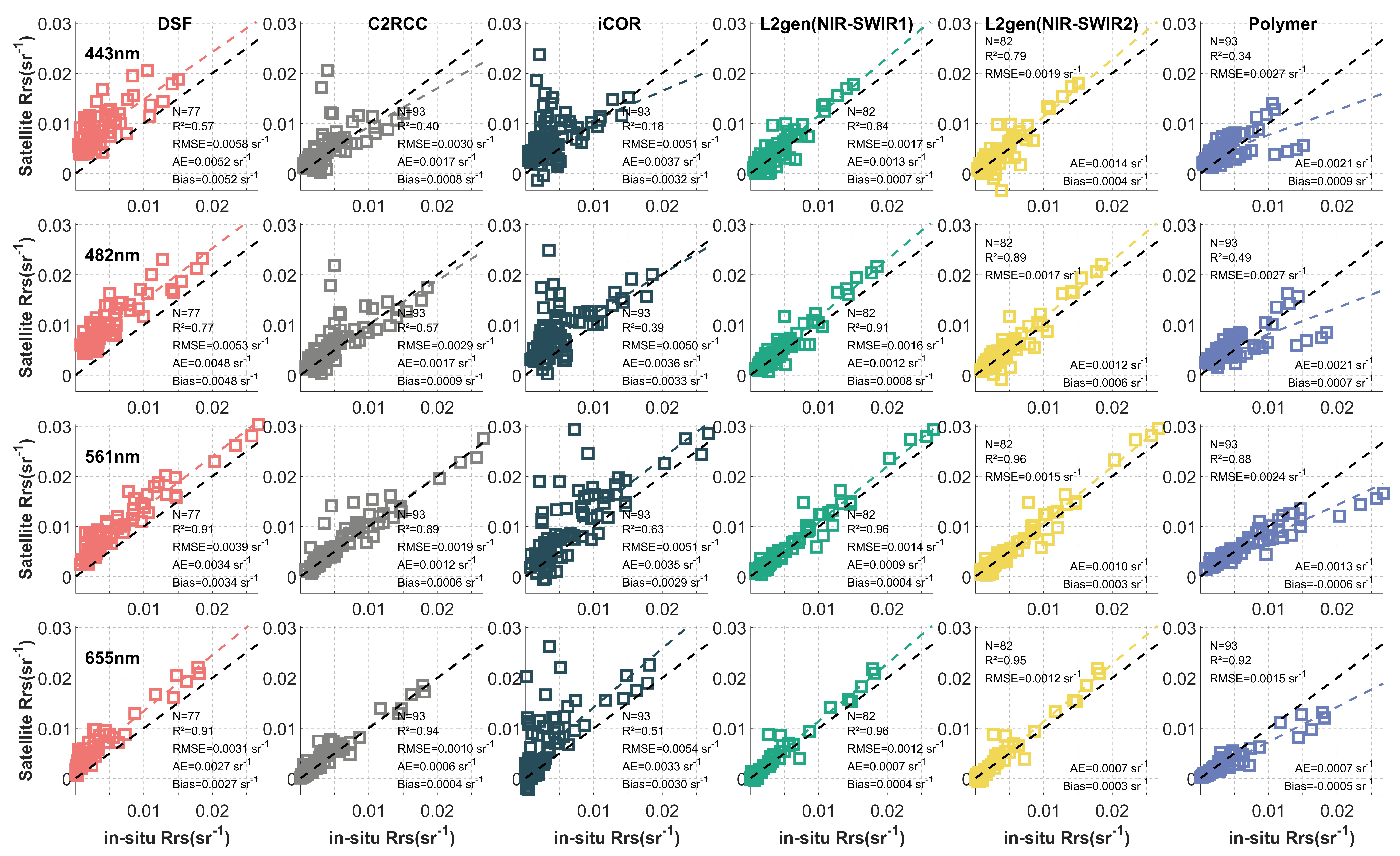
3.1. Error Statistical Analysis of Different AC Methods
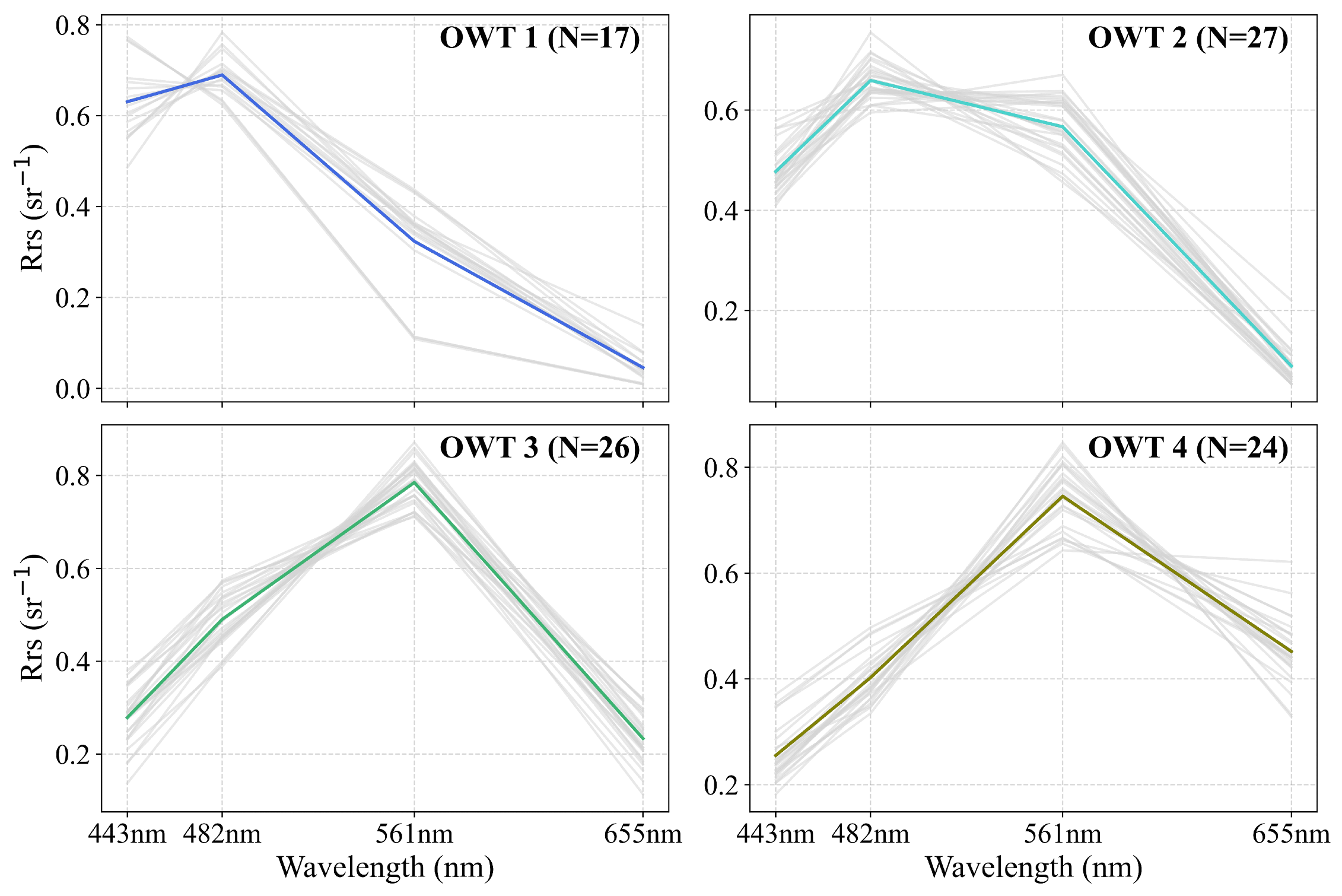
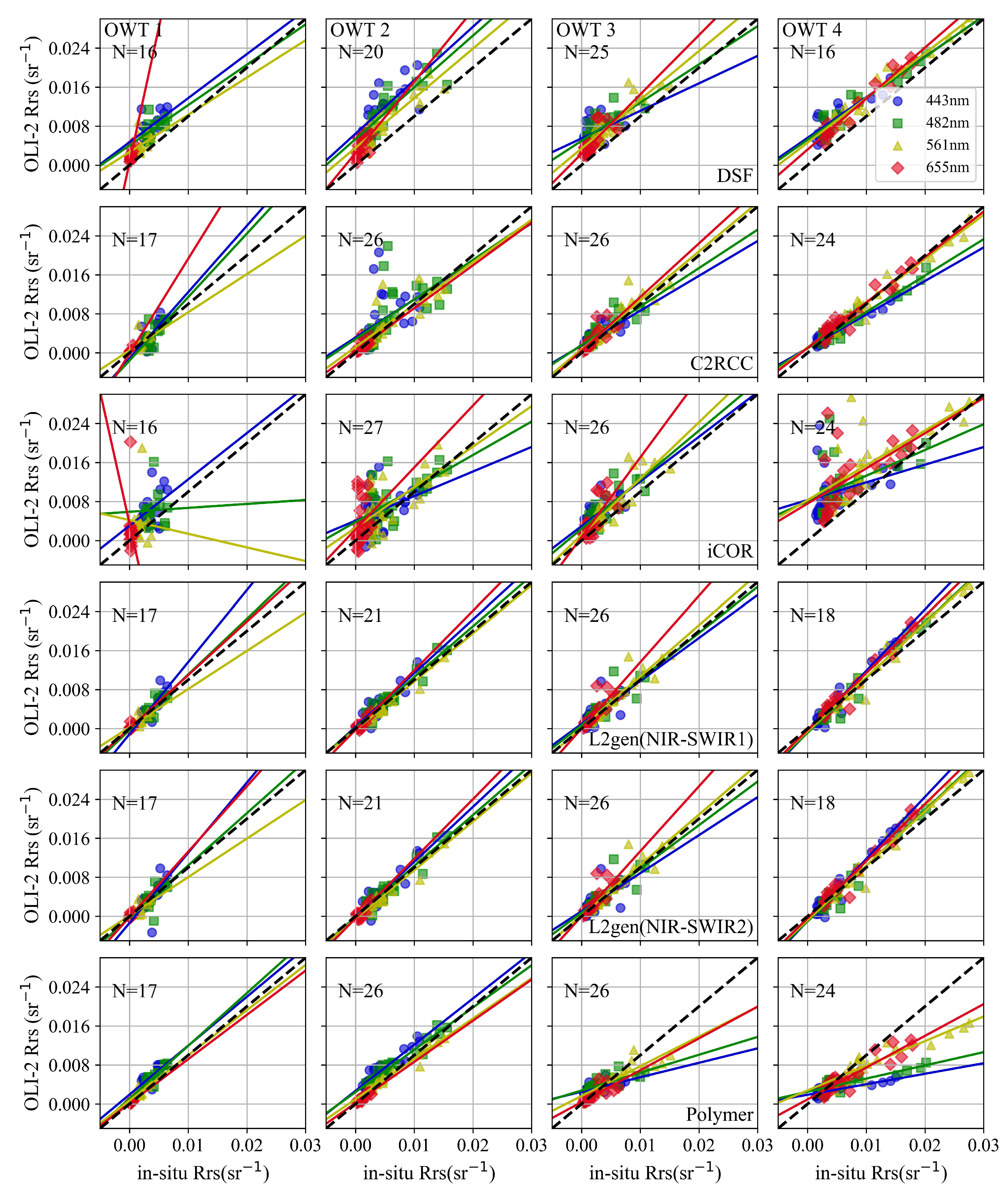
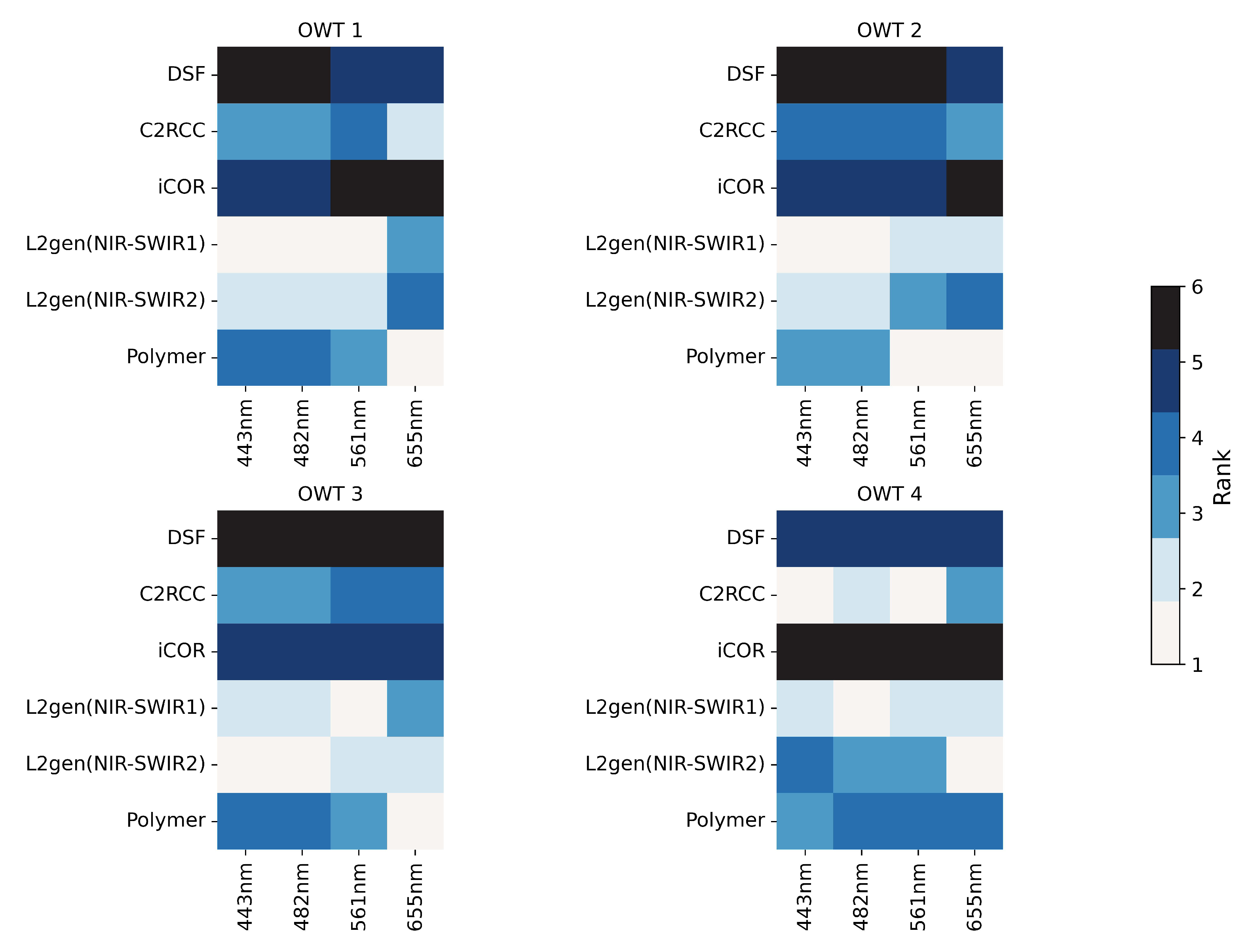
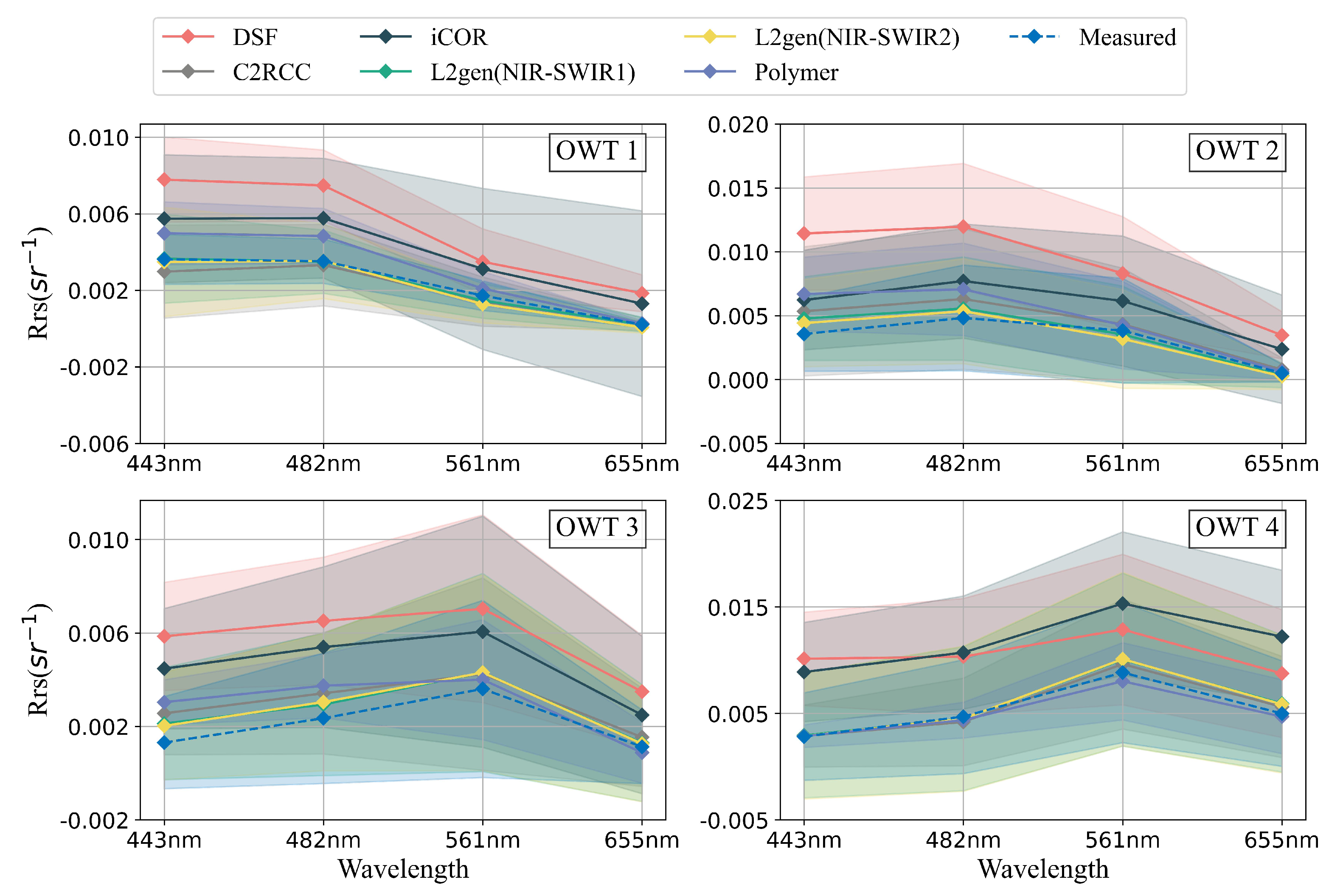
3.2. Performance Variations in AC Methods in Different OWTs
4. Discussion
4.1. Uncertainties of Matchup Analysis
4.2. Analysis of Error Sources of Different AC Methods
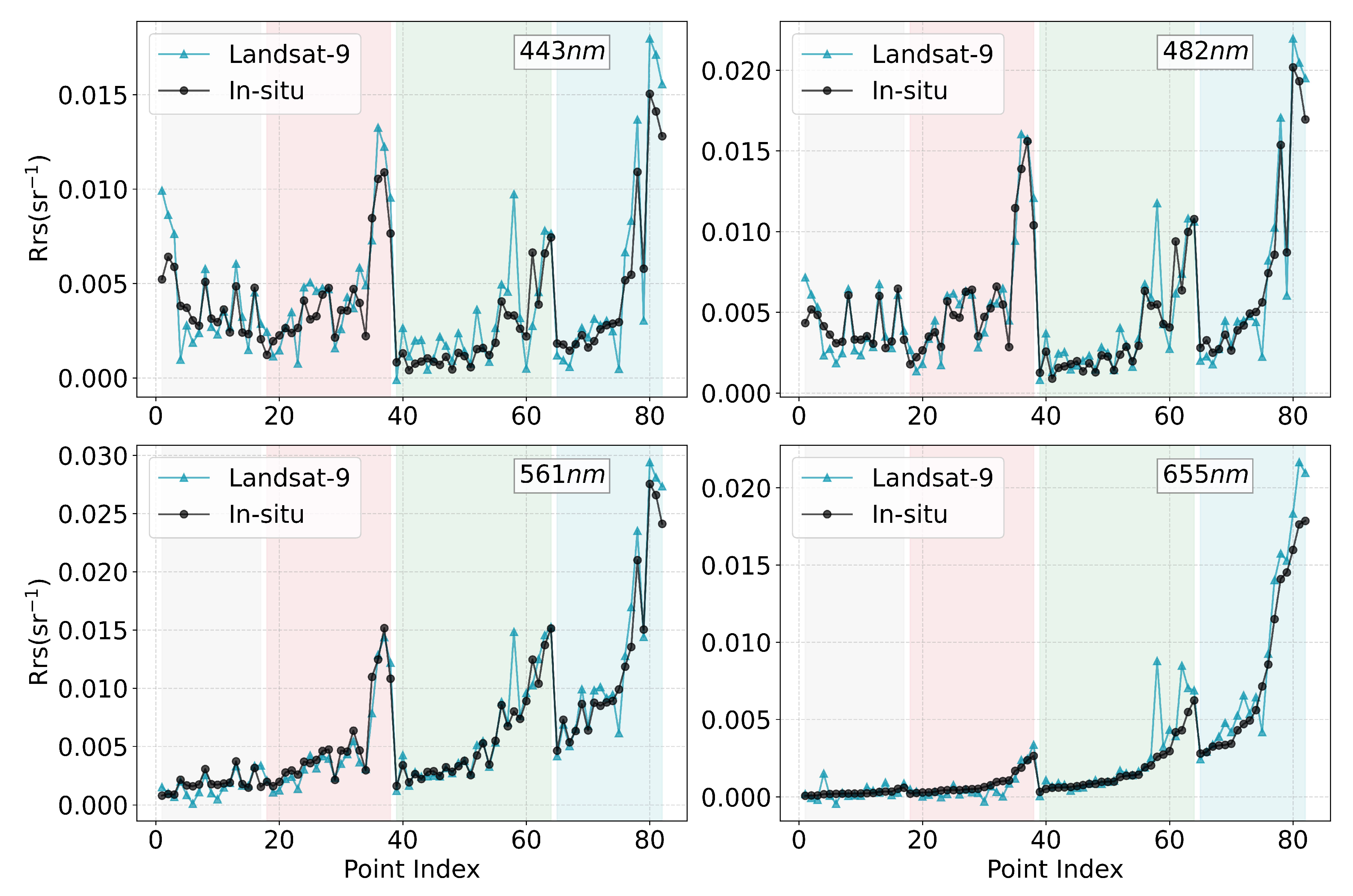
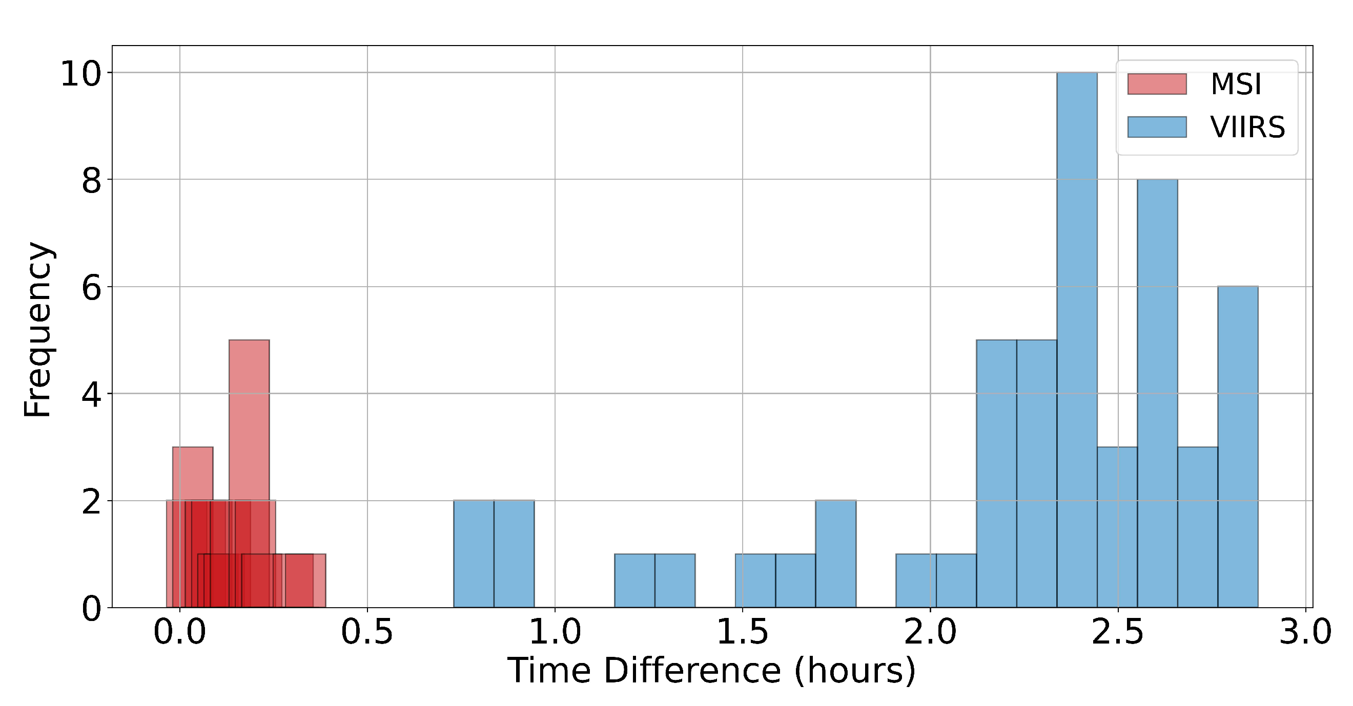
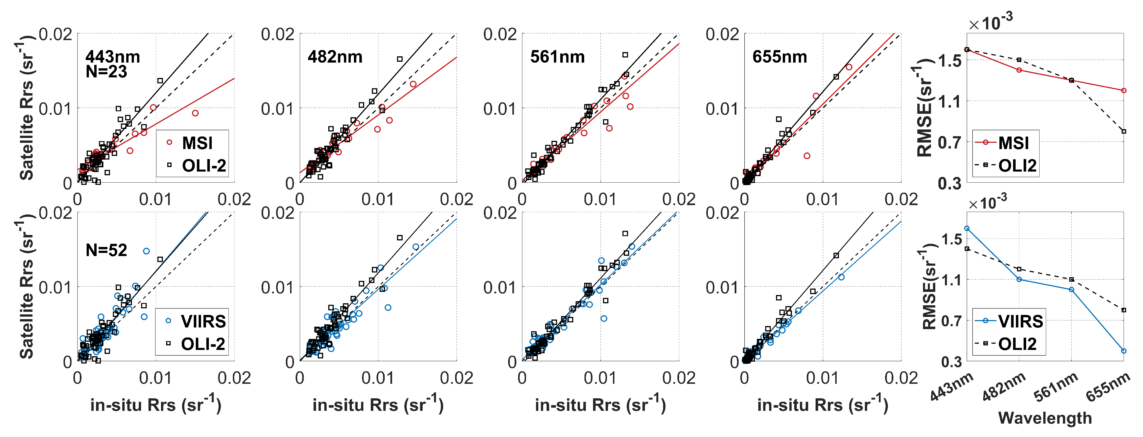
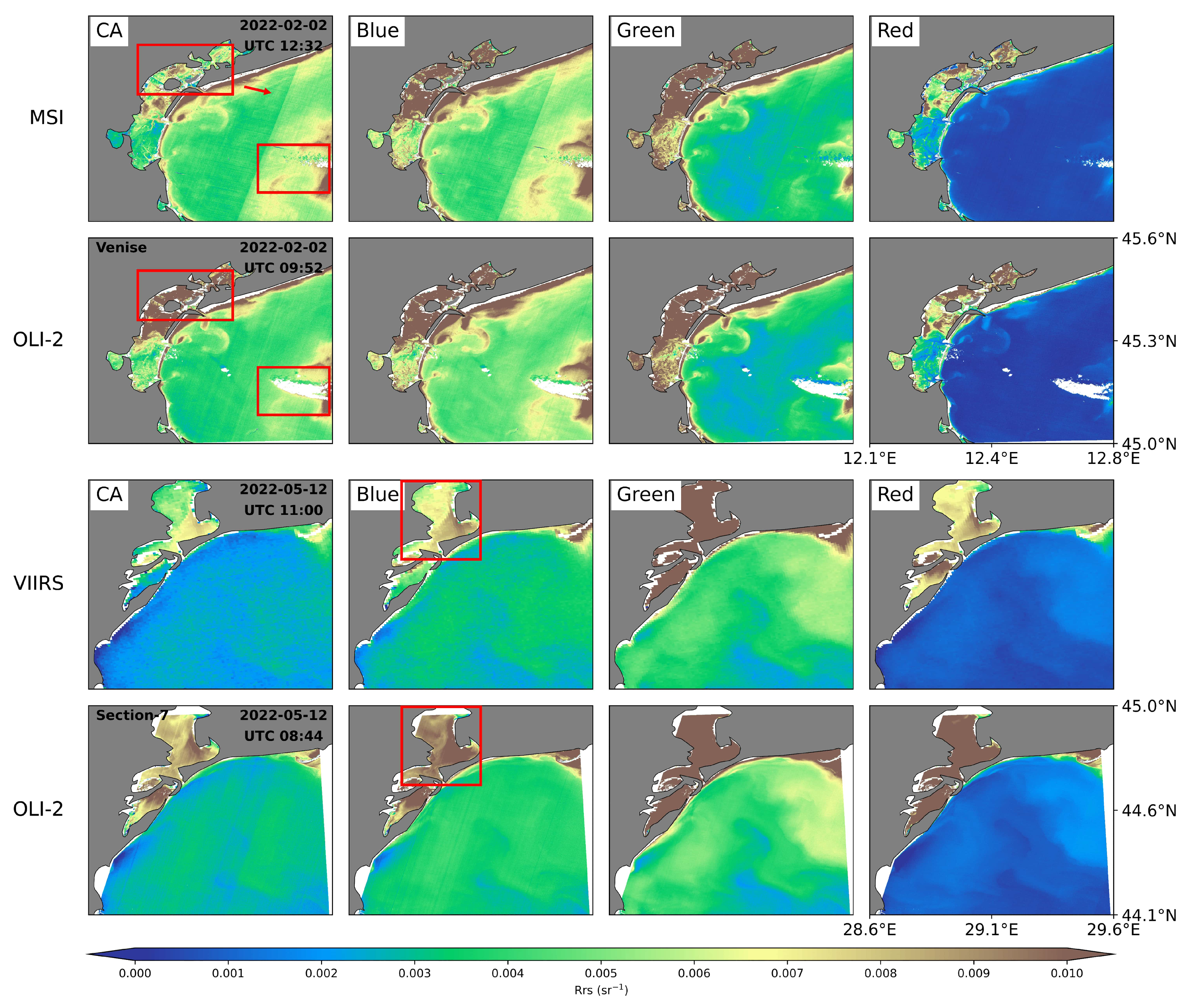
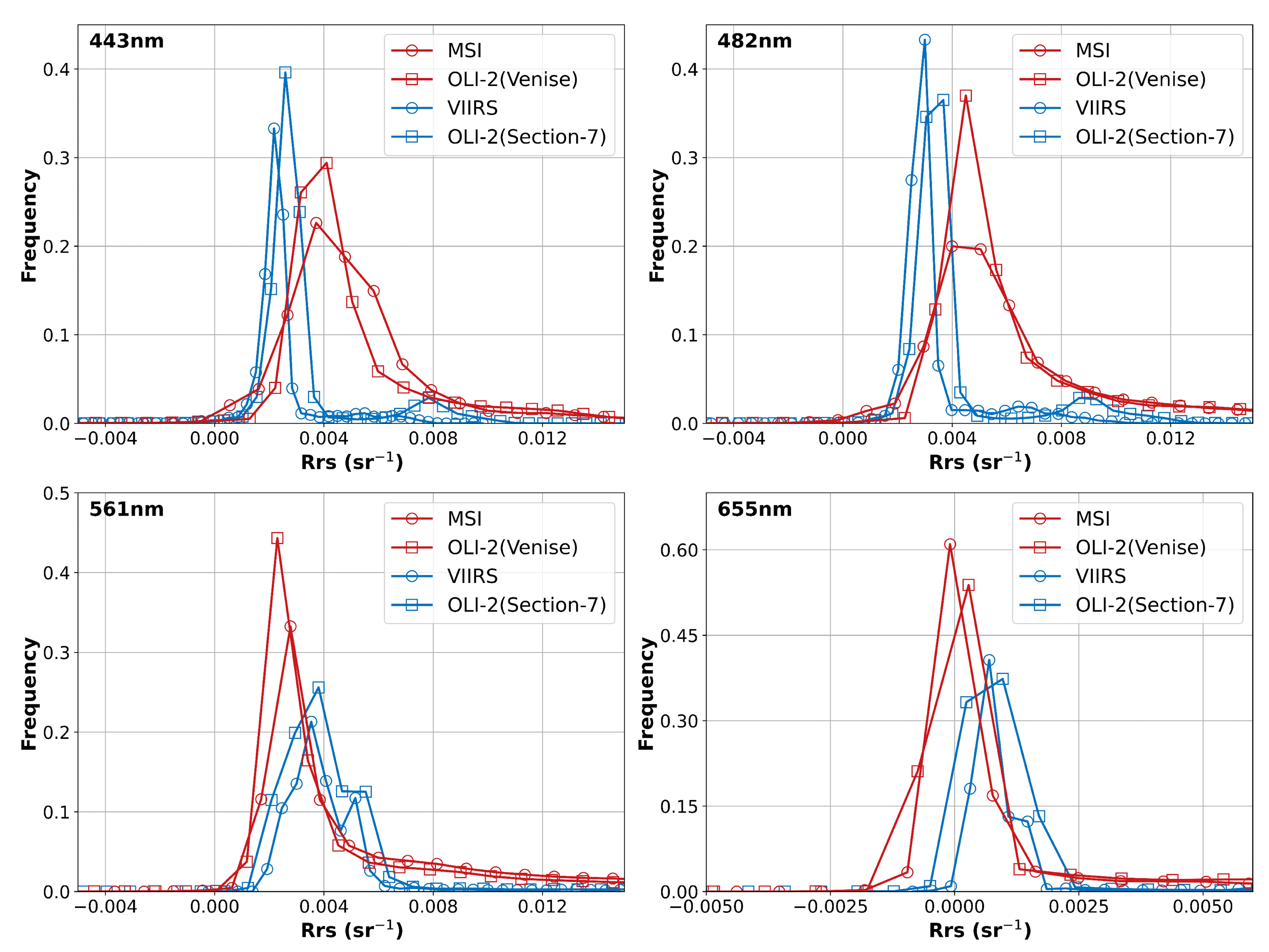
4.3. Consistency Analysis of OLI-2/Landsat-9 with Other On-Orbit Remote Sensing Sensors
5. Conclusions
Supplementary Materials
Author Contributions
Funding
Data Availability Statement
Acknowledgments
Conflicts of Interest
References
- Wulder, M.A.; Roy, D.P.; Radeloff, V.C.; Loveland, T.R.; Anderson, M.C.; Johnson, D.M.; Healey, S.; Zhu, Z.; Scambos, T.A.; Pahlevan, N.; et al. Fifty years of Landsat science and impacts. Remote Sens. Environ. 2022, 280, 113195. [Google Scholar] [CrossRef]
- Kabir, S.; Pahlevan, N.; O’Shea, R.E.; Barnes, B.B. Leveraging Landsat-8/-9 underfly observations to evaluate consistency in reflectance products over aquatic environments. Remote Sens. Environ. 2023, 296, 113755. [Google Scholar] [CrossRef]
- Masek, J.G.; Wulder, M.A.; Markham, B.; McCorkel, J.; Crawford, C.J.; Storey, J.; Jenstrom, D.T. Landsat 9: Empowering open science and applications through continuity. Remote Sens. Environ. 2020, 248, 111968. [Google Scholar] [CrossRef]
- Goward, S.N.; Williams, D.L. Landsat and earth systems science: Development of terrestrial monitoring. Photogramm. Eng. Remote Sens. 1997, 63, 887–900. [Google Scholar]
- Cao, Z.; Ma, R.; Duan, H.; Pahlevan, N.; Melack, J.; Shen, M.; Xue, K. A machine learning approach to estimate chlorophyll-a from Landsat-8 measurements in inland lakes. Remote Sens. Environ. 2020, 248, 111974. [Google Scholar] [CrossRef]
- Chen, Q.; Huang, M.; Tang, X. Eutrophication assessment of seasonal urban lakes in China Yangtze River Basin using Landsat 8-derived Forel-Ule index: A six-year (2013–2018) observation. Sci. Total Environ. 2020, 745, 135392. [Google Scholar] [CrossRef] [PubMed]
- Maleki, S.; Mohajeri, S.H.; Mehraein, M.; Sharafati, A. Lake evaporation in arid zones: Leveraging Landsat 8’s water temperature retrieval and key meteorological drivers. J. Environ. Manag. 2024, 355, 120450. [Google Scholar] [CrossRef]
- Marchese, F.; Genzano, N.; Nolde, M.; Falconieri, A.; Pergola, N.; Plank, S. Mapping and characterizing the Kīlauea (Hawaii) lava lake through Sentinel-2 MSI and Landsat-8 OLI observations of December 2020–February 2021. Environ. Model. Softw. 2022, 148, 105273. [Google Scholar] [CrossRef]
- Chen, J.; Zhu, W.; Tian, Y.Q.; Yu, Q. Monitoring dissolved organic carbon by combining Landsat-8 and Sentinel-2 satellites: Case study in Saginaw River estuary, Lake Huron. Sci. Total Environ. 2020, 718, 137374. [Google Scholar] [CrossRef]
- Li, H.; Li, H.; Wang, J.; Hao, X. Revealing the river ice phenology on the Tibetan Plateau using Sentinel-2 and Landsat 8 overlapping orbit imagery. J. Hydrol. 2023, 619, 129285. [Google Scholar] [CrossRef]
- Osadchiev, A.; Sedakov, R. Spreading dynamics of small river plumes off the northeastern coast of the Black Sea observed by Landsat 8 and Sentinel-2. Remote Sens. Environ. 2019, 221, 522–533. [Google Scholar] [CrossRef]
- Min, Y.; Cui, L.; Li, J.; Han, Y.; Zhuo, Z.; Yin, X.; Zhou, D.; Ke, Y. Detection of large-scale Spartina alterniflora removal in coastal wetlands based on Sentinel-2 and Landsat 8 imagery on Google Earth Engine. Int. J. Appl. Earth Obs. Geoinf. 2023, 125, 103567. [Google Scholar] [CrossRef]
- Pacheco, A.; Horta, J.; Loureiro, C.; Ferreira, Ó. Retrieval of nearshore bathymetry from Landsat 8 images: A tool for coastal monitoring in shallow waters. Remote Sens. Environ. 2015, 159, 102–116. [Google Scholar] [CrossRef]
- Zeng, J.; Sun, Y.; Cao, P.; Wang, H. A phenology-based vegetation index classification (PVC) algorithm for coastal salt marshes using Landsat 8 images. Int. J. Appl. Earth Obs. Geoinf. 2022, 110, 102776. [Google Scholar] [CrossRef]
- Zhang, X.; Xiao, X.; Qiu, S.; Xu, X.; Wang, X.; Chang, Q.; Wu, J.; Li, B. Quantifying latitudinal variation in land surface phenology of Spartina alterniflora saltmarshes across coastal wetlands in China by Landsat 7/8 and Sentinel-2 images. Remote Sens. Environ. 2022, 269, 112810. [Google Scholar] [CrossRef]
- Xu, Y.; Feng, L.; Zhao, D.; Lu, J. Assessment of Landsat atmospheric correction methods for water color applications using global AERONET-OC data. Int. J. Appl. Earth Obs. Geoinf. 2020, 93, 102192. [Google Scholar] [CrossRef]
- Micijevic, E.; Barsi, J.; Haque, M.O.; Levy, R.; Anderson, C.; Thome, K.; Czapla-Myers, J.; Helder, D. Radiometric performance of the Landsat 9 Operational Land Imager over the first 8 months on orbit. In Proceedings of the Earth Observing Systems XXVII, San Diego, CA, USA, 23–25 August 2022; SPIE: Bellingham, DC, USA, 2022; Volume 12232, pp. 249–256. [Google Scholar]
- Gordon, H.R.; Clark, D.K.; Hovis, W.A.; Austin, R.W.; Yentsch, C.S. Ocean color measurements. In Advances in Geophysics; Elsevier: Amsterdam, The Netherlands, 1985; Volume 27, pp. 297–333. [Google Scholar]
- Gordon, H.R. Atmospheric correction of ocean color imagery in the Earth Observing System era. J. Geophys. Res. Atmos. 1997, 102, 17081–17106. [Google Scholar] [CrossRef]
- Gordon, H.R.; Wang, M. Retrieval of water-leaving radiance and aerosol optical thickness over the oceans with SeaWiFS: A preliminary algorithm. Appl. Opt. 1994, 33, 443–452. [Google Scholar] [CrossRef]
- Liu, H.; Li, Q.; Zhu, P.; Hu, Z.; Yang, C.; Wang, Y.; Cui, A.; Wang, Z.; Wu, G. A glimpse of ocean color remote sensing from moon-based Earth observations. IEEE Trans. Geosci. Remote Sens. 2022, 60, 1–11. [Google Scholar] [CrossRef]
- Bailey, S.W.; Franz, B.A.; Werdell, P.J. Estimation of near-infrared water-leaving reflectance for satellite ocean color data processing. Opt. Express 2010, 18, 7521–7527. [Google Scholar] [CrossRef]
- Vanhellemont, Q.; Ruddick, K. Atmospheric correction of Sentinel-3/OLCI data for mapping of suspended particulate matter and chlorophyll-a concentration in Belgian turbid coastal waters. Remote Sens. Environ. 2021, 256, 112284. [Google Scholar] [CrossRef]
- Brockmann, C.; Doerffer, R.; Peters, M.; Kerstin, S.; Embacher, S.; Ruescas, A. Evolution of the C2RCC neural network for Sentinel 2 and 3 for the retrieval of ocean colour products in normal and extreme optically complex waters. In Proceedings of the Living Planet Symposium, Prague, Czech Republic, 9–13 May 2016; Volume 740, p. 54. [Google Scholar]
- Steinmetz, F.; Deschamps, P.Y.; Ramon, D. Atmospheric correction in presence of sun glint: Application to MERIS. Opt. Express 2011, 19, 9783–9800. [Google Scholar] [CrossRef] [PubMed]
- Lee, Z.; Casey, B.; Arnone, R.A.; Weidemann, A.D.; Parsons, R.; Montes, M.J.; Gao, B.C.; Goode, W.; Davis, C.O.; Dye, J. Water and bottom properties of a coastal environment derived from Hyperion data measured from the EO-1 spacecraft platform. J. Appl. Remote Sens. 2007, 1, 011502. [Google Scholar]
- De Keukelaere, L.; Sterckx, S.; Adriaensen, S.; Knaeps, E.; Reusen, I.; Giardino, C.; Bresciani, M.; Hunter, P.; Neil, C.; Van der Zande, D.; et al. Atmospheric correction of Landsat-8/OLI and Sentinel-2/MSI data using iCOR algorithm: Validation for coastal and inland waters. Eur. J. Remote Sens. 2018, 51, 525–542. [Google Scholar] [CrossRef]
- Clewley, D.; Bunting, P.; Shepherd, J.; Gillingham, S.; Flood, N.; Dymond, J.; Lucas, R.; Armston, J.; Moghaddam, M. A python-based open source system for geographic object-based image analysis (GEOBIA) utilizing raster attribute tables. Remote Sens. 2014, 6, 6111–6135. [Google Scholar] [CrossRef]
- Vermote, E.; Justice, C.; Claverie, M.; Franch, B. Preliminary analysis of the performance of the Landsat 8/OLI land surface reflectance product. Remote Sens. Environ. 2016, 185, 46–56. [Google Scholar] [CrossRef]
- Pahlevan, N.; Schott, J.R.; Franz, B.A.; Zibordi, G.; Markham, B.; Bailey, S.; Schaaf, C.B.; Ondrusek, M.; Greb, S.; Strait, C.M. Landsat 8 remote sensing reflectance (Rrs) products: Evaluations, intercomparisons, and enhancements. Remote Sens. Environ. 2017, 190, 289–301. [Google Scholar] [CrossRef]
- Wei, J.; Lee, Z.; Garcia, R.; Zoffoli, L.; Armstrong, R.A.; Shang, Z.; Sheldon, P.; Chen, R.F. An assessment of Landsat-8 atmospheric correction schemes and remote sensing reflectance products in coral reefs and coastal turbid waters. Remote Sens. Environ. 2018, 215, 18–32. [Google Scholar] [CrossRef]
- Ilori, C.O.; Pahlevan, N.; Knudby, A. Analyzing performances of different atmospheric correction techniques for Landsat 8: Application for coastal remote sensing. Remote Sens. 2019, 11, 469. [Google Scholar] [CrossRef]
- Pahlevan, N.; Balasubramanian, S.V.; Sarkar, S.; Franz, B.A. Toward long-term aquatic science products from heritage Landsat missions. Remote Sens. 2018, 10, 1337. [Google Scholar] [CrossRef]
- Yan, N.; Sun, Z.; Huang, W.; Jun, Z.; Sun, S. Assessing Landsat-8 atmospheric correction schemes in low to moderate turbidity waters from a global perspective. Int. J. Digit. Earth 2023, 16, 66–92. [Google Scholar] [CrossRef]
- Van Nguyen, M.; La, O.; Nguyen, H.; Heriza, D.; Lin, B.Y.; Ryadi, G.; Lin, C.H.; Pham, V.Q. Landsat 8 OLI atmospheric correction neural network for inland waters in tropical regions. Int. J. Environ. Sci. Technol. 2024, 1–20. [Google Scholar] [CrossRef]
- Li, J.; Roy, D.P. A global analysis of Sentinel-2A, Sentinel-2B and Landsat-8 data revisit intervals and implications for terrestrial monitoring. Remote Sens. 2017, 9, 902. [Google Scholar] [CrossRef]
- Wu, Z.; Snyder, G.; Vadnais, C.; Arora, R.; Babcock, M.; Stensaas, G.; Doucette, P.; Newman, T. User needs for future Landsat missions. Remote Sens. Environ. 2019, 231, 111214. [Google Scholar] [CrossRef]
- Li, J.; Chen, B. Global revisit interval analysis of Landsat-8-9 and Sentinel-2A-2B data for terrestrial monitoring. Sensors 2020, 20, 6631. [Google Scholar] [CrossRef]
- Pahlevan, N.; Sarkar, S.; Franz, B.A.; Balasubramanian, S.V.; He, J. Sentinel-2 MultiSpectral Instrument (MSI) data processing for aquatic science applications: Demonstrations and validations. Remote Sens. Environ. 2017, 201, 47–56. [Google Scholar] [CrossRef]
- Trevisiol, F.; Mandanici, E.; Pagliarani, A.; Bitelli, G. Evaluation of Landsat-9 interoperability with Sentinel-2 and Landsat-8 over Europe and local comparison with field surveys. ISPRS J. Photogramm. Remote Sens. 2024, 210, 55–68. [Google Scholar] [CrossRef]
- Gilerson, A.; Malinowski, M.; Agagliate, J.; Herrera-Estrella, E.; Tzortziou, M.; Tomlinson, M.C.; Meredith, A.; Stumpf, R.P.; Ondrusek, M.; Jiang, L.; et al. Development of VIIRS-OLCI chlorophyll-a product for the coastal estuaries. Front. Mar. Sci. 2024, 11, 1476425. [Google Scholar] [CrossRef]
- Jiang, G.; Loiselle, S.A.; Yang, D.; Ma, R.; Su, W.; Gao, C. Remote estimation of chlorophyll a concentrations over a wide range of optical conditions based on water classification from VIIRS observations. Remote Sens. Environ. 2020, 241, 111735. [Google Scholar] [CrossRef]
- Cao, Z.; Wang, M.; Ma, R.; Zhang, Y.; Duan, H.; Jiang, L.; Xue, K.; Xiong, J.; Hu, M. A decade-long chlorophyll-a data record in lakes across China from VIIRS observations. Remote Sens. Environ. 2024, 301, 113953. [Google Scholar] [CrossRef]
- Li, S.; Song, K.; Li, Y.; Liu, G.; Wen, Z.; Shang, Y.; Lyu, L.; Fang, C. Performances of atmospheric correction processors for sentinel-2 MSI imagery over typical lakes across China. IEEE J. Sel. Top. Appl. Earth Obs. Remote Sens. 2023, 16, 2065–2078. [Google Scholar] [CrossRef]
- Warren, M.A.; Simis, S.G.; Martinez-Vicente, V.; Poser, K.; Bresciani, M.; Alikas, K.; Spyrakos, E.; Giardino, C.; Ansper, A. Assessment of atmospheric correction algorithms for the Sentinel-2A MultiSpectral Imager over coastal and inland waters. Remote Sens. Environ. 2019, 225, 267–289. [Google Scholar] [CrossRef]
- Sòria-Perpinyà, X.; Delegido, J.; Urrego, E.P.; Ruíz-Verdú, A.; Soria, J.M.; Vicente, E.; Moreno, J. Assessment of sentinel-2-MSI atmospheric correction processors and in situ spectrometry waters quality algorithms. Remote Sens. 2022, 14, 4794. [Google Scholar] [CrossRef]
- Barnes, B.B.; Cannizzaro, J.P.; English, D.C.; Hu, C. Validation of VIIRS and MODIS reflectance data in coastal and oceanic waters: An assessment of methods. Remote Sens. Environ. 2019, 220, 110–123. [Google Scholar] [CrossRef]
- Pardo, S.; Tilstone, G.H.; Brewin, R.J.; Dall’Olmo, G.; Lin, J.; Nencioli, F.; Evers-King, H.; Casal, T.G.; Donlon, C.J. Radiometric assessment of OLCI, VIIRS, and MODIS using fiducial reference measurements along the Atlantic Meridional Transect. Remote Sens. Environ. 2023, 299, 113844. [Google Scholar] [CrossRef]
- Zibordi, G.; Holben, B.; Hooker, S.B.; Mélin, F.; Berthon, J.F.; Slutsker, I.; Giles, D.; Vandemark, D.; Feng, H.; Rutledge, K.; et al. A network for standardized ocean color validation measurements. Eos, Trans. Am. Geophys. Union 2006, 87, 293–297. [Google Scholar] [CrossRef]
- Zibordi, G.; Mélin, F.; Berthon, J.F.; Holben, B.; Slutsker, I.; Giles, D.; D’Alimonte, D.; Vandemark, D.; Feng, H.; Schuster, G.; et al. AERONET-OC: A network for the validation of ocean color primary products. J. Atmos. Ocean. Technol. 2009, 26, 1634–1651. [Google Scholar] [CrossRef]
- Pahlevan, N.; Mangin, A.; Balasubramanian, S.V.; Smith, B.; Alikas, K.; Arai, K.; Barbosa, C.; Bélanger, S.; Binding, C.; Bresciani, M.; et al. ACIX-Aqua: A global assessment of atmospheric correction methods for Landsat-8 and Sentinel-2 over lakes, rivers, and coastal waters. Remote Sens. Environ. 2021, 258, 112366. [Google Scholar] [CrossRef]
- Zhang, M.; Hu, C. Evaluation of remote sensing reflectance derived from the Sentinel-2 multispectral instrument observations using POLYMER atmospheric correction. IEEE Trans. Geosci. Remote Sens. 2020, 58, 5764–5771. [Google Scholar] [CrossRef]
- Clark, D.K.; Feinholz, M.; Yarbrough, M.; Johnson, B.C.; Brown, S.W.; Kim, Y.S.; Barnes, R.A. Overview of the radiometric calibration of MOBY. In Proceedings of the Earth Observing Systems VI, San Diego, CA, USA, 1–3 August 2002; SPIE: Bellingham, DC, USA, 2002; Volume 4483, pp. 64–76. [Google Scholar]
- Clark, D.; Gordon, H.; Voss, K.; Ge, Y.; Broenkow, W.; Trees, C. Validation of atmospheric correction over the oceans. J. Geophys. Res. Atmos. 1997, 102, 17209–17217. [Google Scholar] [CrossRef]
- Valente, A.; Sathyendranath, S.; Brotas, V.; Groom, S.; Grant, M.; Jackson, T.; Chuprin, A.; Taberner, M.; Airs, R.; Antoine, D.; et al. A compilation of global bio-optical in situ data for ocean-colour satellite applications–version three. Earth Syst. Sci. Data Discuss. 2022, 2022, 1–61. [Google Scholar] [CrossRef]
- Thuillier, G.; Floyd, L.; Woods, T.; Cebula, R.; Hilsenrath, E.; Hersé, M.; Labs, D. Solar irradiance reference spectra for two solar active levels. Adv. Space Res. 2004, 34, 256–261. [Google Scholar] [CrossRef]
- Ruddick, K.G.; De Cauwer, V.; Park, Y.J.; Moore, G. Seaborne measurements of near infrared water-leaving reflectance: The similarity spectrum for turbid waters. Limnol. Oceanogr. 2006, 51, 1167–1179. [Google Scholar] [CrossRef]
- Berk, A.; Anderson, G.P.; Acharya, P.K.; Bernstein, L.S.; Muratov, L.; Lee, J.; Fox, M.; Adler-Golden, S.M.; Chetwynd, J.H., Jr.; Hoke, M.L.; et al. MODTRAN5: 2006 update. In Proceedings of the Algorithms and Technologies for Multispectral, Hyperspectral, and Ultraspectral Imagery XII, Kissimmee, UK, 17–20 April 2006; SPIE: Bellingham, DC, USA, 2006; Volume 6233, pp. 508–515. [Google Scholar]
- Ahmad, Z.; Fraser, R.S. An iterative radiative transfer code for ocean-atmosphere systems. J. Atmos. Sci. 1982, 39, 656–665. [Google Scholar] [CrossRef]
- Vanhellemont, Q. Adaptation of the dark spectrum fitting atmospheric correction for aquatic applications of the Landsat and Sentinel-2 archives. Remote Sens. Environ. 2019, 225, 175–192. [Google Scholar] [CrossRef]
- Vanhellemont, Q.; Ruddick, K. Atmospheric correction of metre-scale optical satellite data for inland and coastal water applications. Remote Sens. Environ. 2018, 216, 586–597. [Google Scholar] [CrossRef]
- Franz, B.A.; Bailey, S.W.; Kuring, N.; Werdell, P.J. Ocean color measurements with the Operational Land Imager on Landsat-8: Implementation and evaluation in SeaDAS. J. Appl. Remote Sens. 2015, 9, 096070. [Google Scholar] [CrossRef]
- Steinmetz, F.; Ramon, D. Sentinel-2 MSI and Sentinel-3 OLCI consistent ocean colour products using POLYMER. In Proceedings of the Remote Sensing of the Open and Coastal Ocean and Inland Waters, Honolulu, HI, USA, 24–26 September 2018; SPIE: Bellingham, DC, USA, 2018; Volume 10778, pp. 46–55. [Google Scholar]
- Zhang, M.; Hu, C.; Cannizzaro, J.; English, D.; Barnes, B.B.; Carlson, P.; Yarbro, L. Comparison of two atmospheric correction approaches applied to MODIS measurements over North American waters. Remote Sens. Environ. 2018, 216, 442–455. [Google Scholar] [CrossRef]
- Keshava, N. Distance metrics and band selection in hyperspectral processing with applications to material identification and spectral libraries. IEEE Trans. Geosci. Remote Sens. 2004, 42, 1552–1565. [Google Scholar] [CrossRef]
- Zhao, X.; Ma, Y.; Xiao, Y.; Liu, J.; Ding, J.; Ye, X.; Liu, R. Atmospheric correction algorithm based on deep learning with spatial-spectral feature constraints for broadband optical satellites: Examples from the HY-1C Coastal Zone Imager. ISPRS J. Photogramm. Remote Sens. 2023, 205, 147–162. [Google Scholar] [CrossRef]
- Pahlevan, N.; Roger, J.C.; Ahmad, Z. Revisiting short-wave-infrared (SWIR) bands for atmospheric correction in coastal waters. Opt. Express 2017, 25, 6015–6035. [Google Scholar] [CrossRef] [PubMed]
- Pereira-Sandoval, M.; Ruescas, A.; Urrego, P.; Ruiz-Verdú, A.; Delegido, J.; Tenjo, C.; Soria-Perpinyà, X.; Vicente, E.; Soria, J.; Moreno, J. Evaluation of atmospheric correction algorithms over Spanish inland waters for sentinel-2 multi spectral imagery data. Remote Sens. 2019, 11, 1469. [Google Scholar] [CrossRef]
- Wei, J.; Lee, Z.; Shang, S. A system to measure the data quality of spectral remote-sensing reflectance of aquatic environments. J. Geophys. Res. Ocean. 2016, 121, 8189–8207. [Google Scholar] [CrossRef]
- Renosh, P.R.; Doxaran, D.; Keukelaere, L.D.; Gossn, J.I. Evaluation of atmospheric correction algorithms for sentinel-2-MSI and sentinel-3-OLCI in highly turbid estuarine waters. Remote Sens. 2020, 12, 1285. [Google Scholar] [CrossRef]
- Gordon, H. Phytoplankton pigment concentrations in the middle Atlantic blight: Comparison between shipdeterminations and Coastal Zone Color Scanner estimates. Appl. Opt. 1983, 27, 862–871. [Google Scholar] [CrossRef]
- Bailey, S.W.; Werdell, P.J. A multi-sensor approach for the on-orbit validation of ocean color satellite data products. Remote Sens. Environ. 2006, 102, 12–23. [Google Scholar] [CrossRef]
- Choi, J.K.; Park, Y.J.; Ahn, J.H.; Lim, H.S.; Eom, J.; Ryu, J.H. GOCI, the world’s first geostationary ocean color observation satellite, for the monitoring of temporal variability in coastal water turbidity. J. Geophys. Res. Ocean. 2012, 117. [Google Scholar] [CrossRef]
- Nezlin, N.P.; DiGiacomo, P.M. Satellite ocean color observations of stormwater runoff plumes along the San Pedro Shelf (southern California) during 1997–2003. Cont. Shelf Res. 2005, 25, 1692–1711. [Google Scholar] [CrossRef]
- Shi, W.; Wang, M. Satellite observations of flood-driven Mississippi River plume in the spring of 2008. Geophys. Res. Lett. 2009, 36. [Google Scholar] [CrossRef]
- Bresciani, M.; Pinardi, M.; Free, G.; Luciani, G.; Ghebrehiwot, S.; Laanen, M.; Peters, S.; Della Bella, V.; Padula, R.; Giardino, C. The use of multisource optical sensors to study phytoplankton spatio-temporal variation in a Shallow Turbid Lake. Water 2020, 12, 284. [Google Scholar] [CrossRef]
- Wang, J.; Lee, Z.; Wei, J.; Du, K. Atmospheric correction in coastal region using same-day observations of different sun-sensor geometries with a revised POLYMER model. Opt. Express 2020, 28, 26953–26976. [Google Scholar] [CrossRef] [PubMed]


| OLI-2 | Wavelength (μm) | SR (m) | MSI | Wavelength (μm) | SR (m) | VIIRS | Wavelength (μm) | SR (m) |
|---|---|---|---|---|---|---|---|---|
| B1 | 0.430–0.450 | 30 | B1 | 0.433–0.453 | 60 | M2 | 0.436–0.454 | 750 |
| B2 | 0.450–0.510 | 30 | B2 | 0.458–0.523 | 10 | M3 | 0.478–0.498 | 750 |
| B3 | 0.533–0.590 | 30 | B3 | 0.543–0.578 | 10 | M4 | 0.545–0.565 | 750 |
| B4 | 0.636–0.673 | 30 | B4 | 0.650–0.680 | 10 | M5 | 0.662–0.682 | 750 |
| No. | Station Name | Latitude | Longitude | PI | N |
|---|---|---|---|---|---|
| 1 | ARIAKE_TOWER | 33.104N | 130.272E | Joji Ishizaka/Kohei Arai | 5 |
| 2 | Bahia Blanca | 39.148S | 61.722W | Hubert Loisel/Paula Pratolongo/Robert Frouin | 4 |
| 3 | Chesapeake Bay | 39.124N | 76.349W | Dirk Aurin | 19 |
| 4 | Galata Platform | 43.045N | 28.193E | Frederic Melin | 5 |
| 5 | Gustav Dalen Tower | 58.594N | 17.467E | Frederic Melin | 7 |
| 6 | Kemigawa Offshore | 35.611N | 140.023E | Hiroto Higa | 6 |
| 7 | Lake Erie | 41.826N | 83.194W | Tim Moore/Steve Ruberg/Menghua Wang | 2 |
| 8 | MOBY | 20.4613N | 157.1101W | NOAA/SJSU | 3 |
| 9 | Palgrunden | 58.755N | 13.152E | Susanne Kratzer | 2 |
| 10 | San Marco Platform | 2.942S | 40.215E | Barbara Bulgarelli | 1 |
| 11 | Section-7 Platform | 44.546N | 29.447E | Barbara Bulgarelli | 10 |
| 12 | South Greenbay | 44.596N | 87.951W | Nima Pahlevan | 3 |
| 13 | USC SEAPRISM | 33.564N | 118.118W | Burton Jones/Matthew Ragan | 12 |
| 14 | Venise | 45.314N | 12.508E | Barbara Bulgarelli | 13 |
| DSF | C2RCC | iCOR | L2gen | Polymer | |
|---|---|---|---|---|---|
| Platform | Acolite 2023.10.23 | SNAP 9.0.0 | VITO 3.0 | SeaDAS 8.3.0 | Polymer v4.17beta2 |
| Rayleigh correction method | LUT built using 6SV | Machine learning method | LUT built using MODTRAN 5 [58] | LUT built using Ahmad and Fraser (1982) [59] | LUT built using SOS |
| Aerosol model | Continental/ Maritime aerosols | Aerosols based on AERONET-OC data | MODTRAN rural models | Aerosols based on AERONET-OC data | NA |
| Aerosol correction method | Dark spectrum fitting [60,61] | Machine learning [24] | Dark target and AOT multi-parameter inversion [27] | Iterative bio-optical estimation model with band ratios of NIR/SWIR [30,62] | Spectral matching [25,63] |
| AC | Band (nm) | Slope | Intercept | RMSE (sr−1) | AE (sr−1) | Bias (sr−1) | SA (°) | N | |
|---|---|---|---|---|---|---|---|---|---|
| DSF | 443 nm | 0.57 | 0.94 | 0.0054 | 0.0058 | 0.0052 | 0.0052 | 11.33 | 77 |
| 482 nm | 0.77 | 1.03 | 0.0047 | 0.0053 | 0.0048 | 0.0048 | |||
| 561 nm | 0.91 | 1.04 | 0.0032 | 0.0039 | 0.0034 | 0.0034 | |||
| 655 nm | 0.91 | 1.10 | 0.0024 | 0.0031 | 0.0027 | 0.0027 | |||
| C2RCC | 443 nm | 0.40 | 0.77 | 0.0016 | 0.0030 | 0.0017 | 0.0008 | 5.74 | 93 |
| 482 nm | 0.57 | 0.87 | 0.0015 | 0.0029 | 0.0017 | 0.0009 | |||
| 561 nm | 0.89 | 0.97 | 0.0008 | 0.0019 | 0.0012 | 0.0006 | |||
| 655 nm | 0.94 | 0.98 | 0.0004 | 0.0010 | 0.0006 | 0.0004 | |||
| iCOR | 443 nm | 0.18 | 0.59 | 0.0048 | 0.0051 | 0.0037 | 0.0032 | 12.96 | 93 |
| 482 nm | 0.39 | 0.80 | 0.0042 | 0.0050 | 0.0036 | 0.0033 | |||
| 561 nm | 0.63 | 1.05 | 0.0026 | 0.0051 | 0.0035 | 0.0029 | |||
| 655 nm | 0.51 | 1.16 | 0.0025 | 0.0054 | 0.0033 | 0.0030 | |||
| L2gen (NIR−SWIR1) | 443 nm | 0.84 | 1.15 | 0.0001 | 0.0017 | 0.0013 | 0.0007 | 6.33 | 82 |
| 482 nm | 0.91 | 1.15 | 0.0001 | 0.0016 | 0.0012 | 0.0008 | |||
| 561 nm | 0.96 | 1.11 | −0.0003 | 0.0014 | 0.0009 | 0.0004 | |||
| 655 nm | 0.96 | 1.14 | 0.0000 | 0.0012 | 0.0007 | 0.0004 | |||
| L2gen (NIR−SWIR2) | 443 nm | 0.79 | 1.14 | −0.0001 | 0.0019 | 0.0014 | 0.0004 | 6.38 | 82 |
| 482 nm | 0.89 | 1.15 | −0.0001 | 0.0017 | 0.0012 | 0.0006 | |||
| 561 nm | 0.96 | 1.12 | −0.0004 | 0.0015 | 0.0010 | 0.0003 | |||
| 655 nm | 0.95 | 1.14 | −0.0001 | 0.0012 | 0.0007 | 0.0003 | |||
| Polymer | 443 nm | 0.34 | 0.49 | 0.0028 | 0.0027 | 0.0021 | 0.0009 | 7.76 | 93 |
| 482 nm | 0.49 | 0.52 | 0.0029 | 0.0027 | 0.0021 | 0.0007 | |||
| 561 nm | 0.88 | 0.63 | 0.0017 | 0.0024 | 0.0013 | −0.0006 | |||
| 655 nm | 0.92 | 0.69 | 0.0003 | 0.0015 | 0.0007 | −0.0005 |
| AC Methods | OWTs | 443 nm | 482 nm | 561 nm | 655 nm | SA (°) | N |
|---|---|---|---|---|---|---|---|
| DSF | OWT1 | 135 | 89 | 150 | 815 | 8.23 | 16 |
| OWT2 | 203 | 123 | 94 | 483 | 11.29 | 20 | |
| OWT3 | 430 | 199 | 90 | 249 | 17.26 | 25 | |
| OWT4 | 173 | 92 | 40 | 64 | 10.86 | 16 | |
| C2RCC | OWT1 | 43 | 33 | 43 | 53 | 4.33 | 17 |
| OWT2 | 85 | 56 | 32 | 64 | 8.47 | 26 | |
| OWT3 | 91 | 47 | 20 | 44 | 7.79 | 26 | |
| OWT4 | 25 | 20 | 12 | 21 | 4.55 | 24 | |
| iCOR | OWT1 | 98 | 75 | 167 | 1494 | 11.06 | 16 |
| OWT2 | 114 | 80 | 88 | 572 | 13.37 | 27 | |
| OWT3 | 230 | 103 | 48 | 138 | 15.73 | 26 | |
| OWT4 | 242 | 131 | 64 | 121 | 11.90 | 24 | |
| L2gen (NIR-SWIR1) | OWT1 | 29 | 19 | 35 | 122 | 6.44 | 17 |
| OWT2 | 42 | 23 | 17 | 54 | 6.35 | 21 | |
| OWT3 | 80 | 32 | 13 | 39 | 9.43 | 26 | |
| OWT4 | 34 | 19 | 12 | 19 | 3.70 | 18 | |
| L2gen (NIR-SWIR2) | OWT1 | 37 | 23 | 38 | 133 | 6.47 | 17 |
| OWT2 | 42 | 24 | 21 | 78 | 7.44 | 21 | |
| OWT3 | 75 | 30 | 13 | 39 | 9.47 | 26 | |
| OWT4 | 37 | 21 | 12 | 19 | 3.59 | 18 | |
| Polymer | OWT1 | 61 | 39 | 40 | 52 | 4.75 | 17 |
| OWT2 | 80 | 44 | 16 | 34 | 9.89 | 26 | |
| OWT3 | 146 | 67 | 16 | 25 | 16.43 | 26 | |
| OWT4 | 37 | 31 | 22 | 24 | 5.99 | 24 |
| Sensor | 443 nm | 482 nm | 561 nm | 655 nm | N |
|---|---|---|---|---|---|
| MSI | 0.0016 | 0.0014 | 0.0013 | 0.0012 | 23 |
| OLI-2 | 0.0016 | 0.0015 | 0.0013 | 0.0008 | |
| VIIRS | 0.0016 | 0.0011 | 0.0010 | 0.0004 | 52 |
| OLI-2 | 0.0014 | 0.0012 | 0.0011 | 0.0008 |
Disclaimer/Publisher’s Note: The statements, opinions and data contained in all publications are solely those of the individual author(s) and contributor(s) and not of MDPI and/or the editor(s). MDPI and/or the editor(s) disclaim responsibility for any injury to people or property resulting from any ideas, methods, instructions or products referred to in the content. |
© 2024 by the authors. Licensee MDPI, Basel, Switzerland. This article is an open access article distributed under the terms and conditions of the Creative Commons Attribution (CC BY) license (https://creativecommons.org/licenses/by/4.0/).
Share and Cite
Sun, A.; He, S.; Gu, Y.; Li, P.; Liu, C.; Ye, G.; Zhou, F. Performance Assessment of Landsat-9 Atmospheric Correction Methods in Global Aquatic Systems. Remote Sens. 2024, 16, 4517. https://doi.org/10.3390/rs16234517
Sun A, He S, Gu Y, Li P, Liu C, Ye G, Zhou F. Performance Assessment of Landsat-9 Atmospheric Correction Methods in Global Aquatic Systems. Remote Sensing. 2024; 16(23):4517. https://doi.org/10.3390/rs16234517
Chicago/Turabian StyleSun, Aoxiang, Shuangyan He, Yanzhen Gu, Peiliang Li, Cong Liu, Guanqiong Ye, and Feng Zhou. 2024. "Performance Assessment of Landsat-9 Atmospheric Correction Methods in Global Aquatic Systems" Remote Sensing 16, no. 23: 4517. https://doi.org/10.3390/rs16234517
APA StyleSun, A., He, S., Gu, Y., Li, P., Liu, C., Ye, G., & Zhou, F. (2024). Performance Assessment of Landsat-9 Atmospheric Correction Methods in Global Aquatic Systems. Remote Sensing, 16(23), 4517. https://doi.org/10.3390/rs16234517