Estimation of Signal Distortion Bias Using Geometry-Free Linear Combinations

Abstract

Signal distortion bias (SDB) in Global Navigation Satellite System (GNSS) data processing, defined as the time difference between the distorted chip and the ideal rectangular chip, leads to systematic biases in pseudoranges, affecting satellite and receiver differential code biases (DCBs). The stability of SDBs, allowing them to be treated as constant values, highlights the importance of investigating both their stability and estimation accuracy. Two different methods are used to estimate SDBs: (1) the hybrid method and (2) the geometry-free method. Data from approximately 430 stations, spanning the entire year of 2021, were analyzed to evaluate the estimation accuracy and the short-term and long-term stability of GPS SDBs. The analysis focused on two code signals: C1C (L1 Coarse/Acquisition) and C2W (L2 P(Y)). The results show that the short-term and long-term stability of GPS C1C and C2W SDBs is comparable for both methods, with only minor variations between them. Additionally, one month of data were used to validate the accuracy of estimated SDBs across different receiver groups. The results demonstrate that geometry-free SDBs provide stable satellite DCB estimates with an average bias below 0.15 ns and minimal residual biases, while hybrid SDBs provide satellite DCB estimates with an average bias below 0.20 ns. Overall, the comparison underscores the superior performance of geometry-free SDBs in achieving consistent satellite DCB estimates.

1. Introduction

The theoretical shape of a chip in GNSS receivers is assumed to be rectangular. However, in practice, the actual shape is distorted, leading to biases in pseudorange measurements [1]. Numerous studies have demonstrated a correlation between these biases, the chip’s shape, and the correlators used [2]. This bias, known as the signal distortion bias (SDB), is defined as the time difference between the distorted chip and the ideal rectangular chip. Consequently, different receiver designs can result in varying SDBs.

SDBs cannot be eliminated by using double- or single- or zero-differences when different sets of receivers are used [3,4]. The SDBs cannot be separated into two parts, satellite-related and receiver-related, because they depend on the satellite–receiver pair [5]. It is possible to estimate SDBs based on receiver brands and models, with receivers of the same brand and model exhibiting identical SDB values. SDBs affect various linear combinations, such as the dual-frequency pseudorange geometry-free (GF) and Melbourne–Wübbena wide-lane (MWWL), which in turn influence the DCB estimation derived from GF linear combinations. SDBs are utilized to improve the consistency and long-term stability of satellite DCBs, resulting in a remarkable 60% improvement in removing the long-term DCB variations [6]. Previous studies have observed biases in satellite DCBs using a network of different receivers [7,8]. Additionally, SDBs play a crucial role in resolving WL ambiguities. Disregarding SDBs can result in positioning errors reaching a maximum of 10 cm [9]. However, through SDB calibration, positioning performance can be enhanced by up to 50%, accompanied by a 10% improvement in the ambiguity fixing rate.

Previous studies have employed various methods to estimate SDBs. The traditional dual-frequency ionosphere-free (IF) observable is only used to estimate the IF SDBs, leveraging its effectiveness in mitigating the first-order ionosphere effect [10]. To remove the satellite bias in IF SDB estimates, a differencing strategy was implemented using a reference receiver. However, this approach has two significant limitations: the estimated SDBs do not accurately represent single-frequency biases and are not relative to broadcast or precise ephemerides. In contrast, undifferenced pseudorange observations are utilized to estimate single-frequency SDBs and incorporated global ionospheric maps to mitigate the first-order ionospheric effect [11]. The zero-mean condition was employed to separate the estimated SDBs. Unfortunately, the undifferenced model is prone to significant ionospheric residuals. Two IF linear combinations and MWWL linear combinations are used to estimate triple-frequency BeiDou SDBs [12]. Similarly, the differencing strategy was employed to remove the satellite biases. However, a limitation of this model is that the estimated SDBs are not compatible with broadcast or precise products. Similarly, the IF dual-frequency linear combination with fixed receiver positions, the triple-frequency pseudorange geometry-free ionosphere-free (GFIF) linear combination, and MWWL linear combinations are used along with zero-mean conditions to separate the estimated SDBs [5]. However, this method exhibits instability in IF code residuals during ambiguity initialization, as the IF receiver clock estimate absorbs the average of the IF SDBs of visible satellites. Consequently, the daily mean IF residuals become biased, impacting the stability and accuracy of SDBs. This method is referred to as a “hybrid method” because it uses geometry-free and geometry-fixed linear combinations together.

In our study, we propose using three GF linear combinations, namely the dual-frequency GF linear combination, the MWWL linear combination, and the triple-frequency GFIF linear combination. This approach aims to improve the stability and estimation accuracy of SDBs by demonstrating consistency in the residuals obtained from these combinations. Section 2 provides a comprehensive overview of the two SDB estimation methods, the hybrid method and the geometry-free method, along with the data used, processing options, and the classification of receiver groups. Section 3 presents the SDB estimates using both methods and their long- and short-term stability. Section 4 discusses the accuracy and validation of estimated SDBs for both methods, demonstrating the stability of satellite DCBs. Finally, Section 5 concludes the study.

2. Materials and Methods

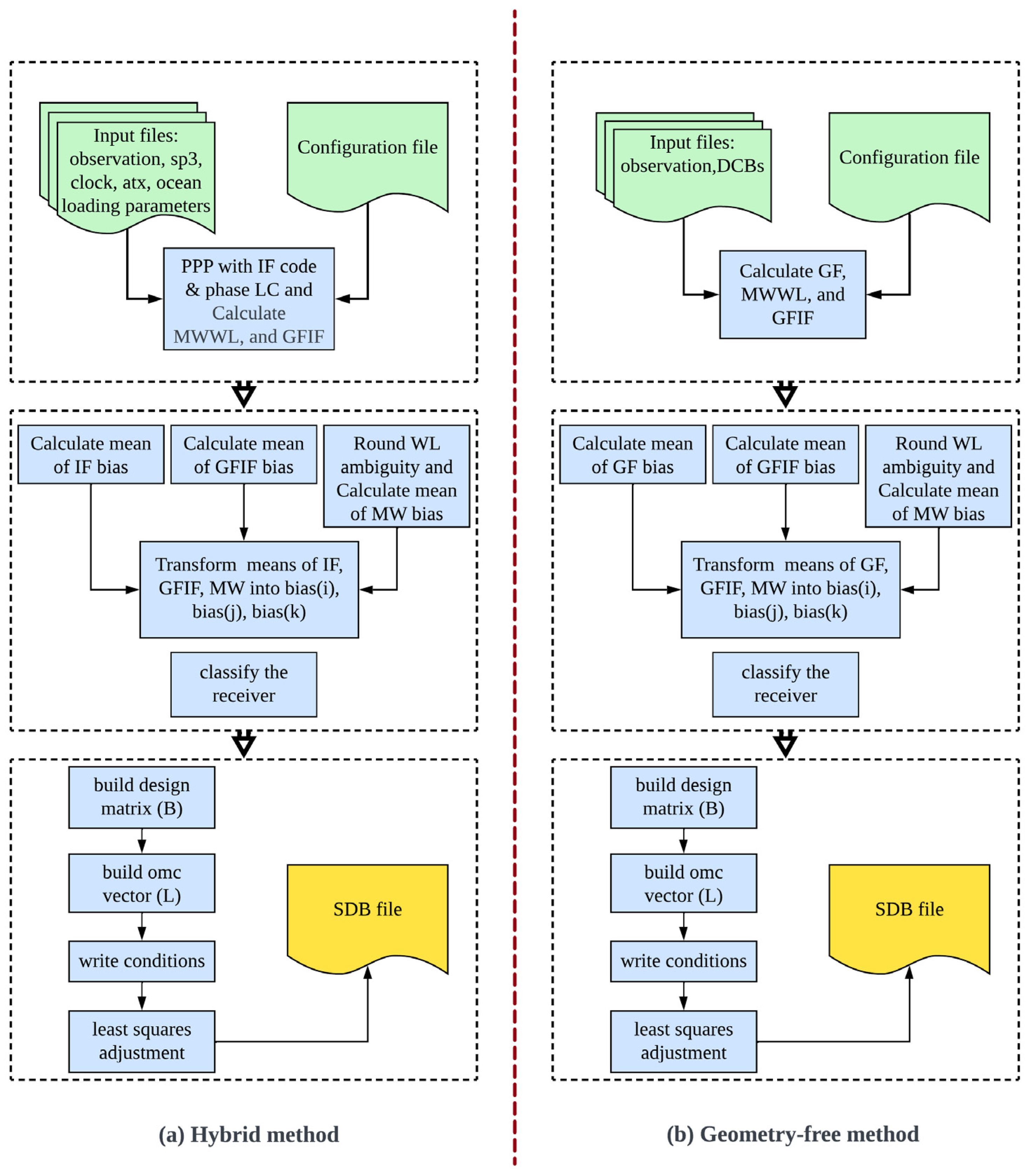
Traditionally, pseudorange hardware biases are separated into two parts: satellite-related bias and receiver-related bias [13]. However, due to the existence of SDB, these hardware biases are now divided into three parts: satellite-related bias, receiver-related bias, and SDB [5,10,12]. The basic measurement equations can be expressed as follows:

$$\begin{array}{l}{P}_{r,sig}^s=\rho +d{t}_r-d{t}^s+mT+{\mu }_{sig}{I}^s+b_{r,sig}-b_{sig}^s+b_{group(r),sig}^s\\ {\mathrm{\Phi }}_{r,sig}^s=\rho +d{t}_r-d{t}^s+mT-{\mu }_{sig}{I}^s+B_{r,sig}-B_{sig}^s+{\lambda }_{sig}{N}_{sig}^s\end{array}$$

(1)

where $P_{r,sig}^s$ and ${\mathrm{\Phi }}_{r,sig}^s$ are the code and phase measurements for a satellite s and a receiver r on a signal sig. $\rho$ represents the geometric distance, while $d{t}_r$ and $d{t}^s$ represent the receiver and satellite clock errors, respectively. Additionally, T refers to the zenith tropospheric effect, while $I^s$ refers to the slant ionospheric effect. m represents the tropospheric mapping function, and ${\mu }_{sig}$ represents the frequency-dependent factor. $b_{r,sig}$ and $b_{sig}^s$ are the pseudorange receiver-related and satellite-related hardware biases, respectively, while $b_{group(r),sig}^s$ is the SDB which is different for each receiver–satellite pair. $B_{r,sig}$ and $B_{sig}^s$ denote carrier-phase receiver-related and satellite-related hardware biases, respectively, while $N_{sig}^s$ and ${\lambda }_{sig}$ denote the ambiguity term and the wavelength, respectively.

2.1. Hybrid Method

This method, proposed by Gong et al. [5], includes one geometry-fixed linear combination and two GF linear combinations for estimating the SDBs: the dual-frequency pseudorange IF linear combination, the MWWL linear combination, and the triple-frequency pseudorange GFIF linear combination. These three linear combinations can be expressed as follows:

$$\begin{array}{l}{P}_{r,IF,sig(x,y)}^s\hspace{0.17em}\hspace{0.17em}\hspace{0.17em}\hspace{0.17em}\hspace{0.17em}\hspace{0.17em}\hspace{0.17em}\hspace{0.17em}={\alpha }_{IF}{P}_{r,sig(x)}^s-{\beta }_{IF}{P}_{r,sig(y)}^s\\ MWW{L}_{r,sig(x,y)}^s\hspace{0.17em}\hspace{0.17em}\hspace{0.17em}={\displaystyle \frac{1}{{\lambda }_{MWWL,sig(x,y)}}}\ast \left({\alpha }_{MWWL}{P}_{r,sig(x)}^s+{\beta }_{MWWL}{P}_{r,sig(y)}^s\right)-\left({\displaystyle \frac{{\mathrm{\Phi }}_{r,sig(x)}^s}{{\lambda }_{sig(x)}}}-{\displaystyle \frac{{\mathrm{\Phi }}_{r,sig(y)}^s}{{\lambda }_{sig(y)}}}\right)\hspace{0.17em}\hspace{0.17em}\\ GFI{F}_{r,sig(x,y,z)}^s\hspace{0.17em}\hspace{0.17em}\hspace{0.17em}\hspace{0.17em}\hspace{0.17em}=({\alpha }_{IF}-{\alpha }_{GFIF})P_{r,sig(x)}^s-{\beta }_{IF}{P}_{r,sig(y)}^s+{\beta }_{GFIF}{P}_{r,sig(z)}^s\end{array}$$

(2)

where $P_{r,IF,sig(x,y)}^s$, $MWW{L}_{r,sig(x,y)}^s$, and $GFI{F}_{r,sig(x,y,z)}^s$ refer to the pseudorange IF linear combination, the MWWL linear combination and the triple-frequency pseudorange GFIF linear combination, respectively. The coefficients are defined as follows:

$${\alpha }_{IF}={\displaystyle \frac{f_{sig(x)}^2}{f_{sig(x)}^2-f_{sig(y)}^2}},$$

$${\beta }_{IF}={\displaystyle \frac{f_{sig(y)}^2}{f_{sig(x)}^2-f_{sig(y)}^2}},$$

$${\alpha }_{MWWL}={\displaystyle \frac{f_{sig(x)}}{f_{sig(x)}+f_{sig(y)}}},$$

$${\beta }_{MWWL}={\displaystyle \frac{f_{sig(y)}}{f_{sig(x)}+f_{sig(y)}}},$$

$${\alpha }_{GFIF}={\displaystyle \frac{f_{sig(x)}^2}{f_{sig(x)}^2-f_{sig(z)}^2}},$$

$${\beta }_{GFIF}={\displaystyle \frac{f_{sig(z)}^2}{f_{sig(x)}^2-f_{sig(z)}^2}}.$$

x denotes the C1C code, y denotes the C2W code, and z denotes the C5X code.

To estimate the SDBs using Equation (2), the geometry-fixed dual-frequency pseudorange IF observable is used, where the geometry term is eliminated by fixing the receiver position. During the ambiguity initialization, the IF receiver clock estimate absorbs the average of the IF SDBs of the visible satellites. As a result, the pseudorange IF residual, which is the difference between the calculated and measured range, includes the satellite IF SDB minus the average of IF SDBs of visible satellites, noise, multipath effects, and residuals of both IF satellite-related and receiver-related pseudorange hardware biases. As a result of using the geometry-fixed IF linear combination, the IF residual no longer retains the characteristic of being a pure IF SDB.

For the first GF linear combination, the MWWL, the WL ambiguity can be resolved through rounding to the nearest integer. Consequently, the MWWL residual includes the MWWL SDB, noise, multipath effects, and residuals of code and phase MWWL satellite-related and receiver-related pseudorange hardware biases. The receiver clock is removed by the geometry-free linear combination, so the MWWL residuals contain only the pure MWWL SDB. The second GF linear combination, known as GFIF, includes a pure GFIF SDB, hardware biases, as well as noise and multipath effects from the GFIF linear combination. The use of geometry-free observables preserves the characteristic of the residuals being consistent SDBs. In summary, these three observables can be formulated as follows:

$$\begin{array}{l}bia{s}_{r,IF,sig(x,y)}^s\hspace{0.17em}\hspace{0.17em}\hspace{0.17em}\hspace{0.17em}\hspace{0.17em}\hspace{0.17em}=P_{cal}-P_{r,IF,sig(x,y)}^s\\ \hspace{0.17em}\hspace{0.17em}\hspace{0.17em}\hspace{0.17em}\hspace{0.17em}\hspace{0.17em}\hspace{0.17em}\hspace{0.17em}\hspace{0.17em}\hspace{0.17em}\hspace{0.17em}\hspace{0.17em}\hspace{0.17em}\hspace{0.17em}\hspace{0.17em}\hspace{0.17em}\hspace{0.17em}\hspace{0.17em}\hspace{0.17em}\hspace{0.17em}={\alpha }_{IF}\ast \left({\overline{b}}_{r,sig(x)}-{\overline{b}}_{sig(x)}^s+b_{group(r),sig(x)}^s-{\displaystyle \frac{1}{m}}{\displaystyle \sum _{s=1}^m{b}_{group(r),sig(x)}^s}\right)\\ \hspace{0.17em}\hspace{0.17em}\hspace{0.17em}\hspace{0.17em}\hspace{0.17em}\hspace{0.17em}\hspace{0.17em}\hspace{0.17em}\hspace{0.17em}\hspace{0.17em}\hspace{0.17em}\hspace{0.17em}\hspace{0.17em}\hspace{0.17em}\hspace{0.17em}\hspace{0.17em}\hspace{0.17em}\hspace{0.17em}\hspace{0.17em}\hspace{0.17em}-{\beta }_{IF}\ast \left({\overline{b}}_{r,sig(y)}-{\overline{b}}_{sig(y)}^s+b_{group(r),sig(y)}^s-{\displaystyle \frac{1}{m}}{\displaystyle \sum _{s=1}^m{b}_{group(r),sig(y)}^s}\right)\\ bia{s}_{r,MWWL,sig(x,y)}^s\hspace{0.17em}={\lambda }_{MWWL,sig(x,y)}\ast \left(MWW{L}_{r,sig(x,y)}^s-round(MWW{L}_{r,sig(x,y)}^s)\right)\hspace{0.17em}\hspace{0.17em}\hspace{0.17em}\hspace{0.17em}\hspace{0.17em}\hspace{0.17em}\hspace{0.17em}\hspace{0.17em}\hspace{0.17em}\hspace{0.17em}\hspace{0.17em}\hspace{0.17em}\hspace{0.17em}\hspace{0.17em}\\ \hspace{0.17em}\hspace{0.17em}\hspace{0.17em}\hspace{0.17em}\hspace{0.17em}\hspace{0.17em}\hspace{0.17em}\hspace{0.17em}\hspace{0.17em}\hspace{0.17em}\hspace{0.17em}\hspace{0.17em}\hspace{0.17em}\hspace{0.17em}\hspace{0.17em}\hspace{0.17em}\hspace{0.17em}\hspace{0.17em}\hspace{0.17em}\hspace{0.17em}={\alpha }_{MWWL}\ast \left({\overline{b}}_{r,sig(x)}-{\overline{b}}_{sig(x)}^s+b_{group(r),sig(y)}^s\right)\\ \hspace{0.17em}\hspace{0.17em}\hspace{0.17em}\hspace{0.17em}\hspace{0.17em}\hspace{0.17em}\hspace{0.17em}\hspace{0.17em}\hspace{0.17em}\hspace{0.17em}\hspace{0.17em}\hspace{0.17em}\hspace{0.17em}\hspace{0.17em}\hspace{0.17em}\hspace{0.17em}\hspace{0.17em}\hspace{0.17em}\hspace{0.17em}\hspace{0.17em}+{\beta }_{MWWL}\ast \left({\overline{b}}_{r,sig(y)}-{\overline{b}}_{sig(y)}^s+b_{group(r),sig(y)}^s\right)+{\overline{B}}_{r,MWWL,sig(x,y)}^s\\ bia{s}_{r,GFIF,sig(x,y,z)}^s\hspace{0.17em}=({\alpha }_{IF}-{\alpha }_{GFIF})\ast bia{s}_{r,sig(x)}^s-{\beta }_{IF}\ast bia{s}_{r,sig(y)}^s+{\beta }_{GFIF}\ast bia{s}_{r,sig(z)}^s\end{array}$$

(3)

where $bia{s}_{r,IF,sig(x,y)}^s$, $bia{s}_{r,MWWL,sig(x,y)}^s$, and $bia{s}_{r,GFIF,sig(x,y,z)}^s$ are the residuals of the IF, MWWL, and GFIF linear combinations, respectively; $P_{cal}$ is the calculated distance between satellite and receiver; ${\overline{b}}_{r,sig}$, ${\overline{b}}_{sig}^s$, and m are the residuals of receiver-related and satellite-related pseudorange hardware biases and the number of visible satellites, respectively; round(*) refers to the integer rounding to fix the WL ambiguity; ${\overline{B}}_{r,MWWL,sig(x,y)}^s$ is the residual of MWWL carrier-phase hardware biases. In order to simplify the estimation of SDBs, it is necessary to separate the SDB for each frequency into a single equation. The residual bias for each frequency can be written as follows:

$$\begin{array}{l}bia{s}_{r,sig(x)}^s\hspace{0.17em}\hspace{0.17em}\hspace{0.17em}={\displaystyle \frac{f_{sig(y)}}{f_{sig(x)}}}bia{s}_{r,MWWL,sig(x,y)}^s-{\displaystyle \frac{f_{sig(x)}-f_{sig(y)}}{f_{sig(x)}}}bia{s}_{r,IF,sig(x,y)}^s\\ bia{s}_{r,sig(y)}^s\hspace{0.17em}\hspace{0.17em}\hspace{0.17em}={\displaystyle \frac{f_{sig(x)}}{f_{sig(y)}}}bia{s}_{r,MWWL,sig(x,y)}^s-{\displaystyle \frac{f_{sig(x)}-f_{sig(y)}}{f_{sig(y)}}}bia{s}_{r,IF,sig(x,y)}^s\hspace{0.17em}\hspace{0.17em}\hspace{0.17em}\hspace{0.17em}\hspace{0.17em}\hspace{0.17em}\hspace{0.17em}\hspace{0.17em}\hspace{0.17em}\hspace{0.17em}\hspace{0.17em}\hspace{0.17em}\hspace{0.17em}\hspace{0.17em}\hspace{0.17em}\hspace{0.17em}\hspace{0.17em}\hspace{0.17em}\hspace{0.17em}\hspace{0.17em}\hspace{0.17em}\hspace{0.17em}\hspace{0.17em}\hspace{0.17em}\hspace{0.17em}\hspace{0.17em}\hspace{0.17em}\hspace{0.17em}\hspace{0.17em}\hspace{0.17em}\hspace{0.17em}\hspace{0.17em}\hspace{0.17em}\hspace{0.17em}\hspace{0.17em}\hspace{0.17em}\hspace{0.17em}\hspace{0.17em}\hspace{0.17em}\hspace{0.17em}\hspace{0.17em}\hspace{0.17em}\hspace{0.17em}\hspace{0.17em}\hspace{0.17em}\hspace{0.17em}\hspace{0.17em}\\ bia{s}_{r,sig(z)}^s\hspace{0.17em}\hspace{0.17em}\hspace{0.17em}={\displaystyle \frac{f_{sig(x)}^2-f_{sig(z)}^2}{f_{sig(z)}^2}}bia{s}_{r,GFIF,sig(x,y,z)}^s+{\displaystyle \frac{f_{sig(x)}{f}_{sig(y)}}{f_{sig(k)}^2}}bia{s}_{r,MWWL,sig(x,y)}^s\\ \hspace{0.17em}\hspace{0.17em}\hspace{0.17em}\hspace{0.17em}\hspace{0.17em}\hspace{0.17em}\hspace{0.17em}\hspace{0.17em}\hspace{0.17em}\hspace{0.17em}\hspace{0.17em}\hspace{0.17em}\hspace{0.17em}+{\displaystyle \frac{f_{sig(z)}^2-f_{sig(x)}{f}_{sig(y)}}{f_{sig(z)}^2}}bia{s}_{r,IF,sig(x,y)}^s\end{array}$$

(4)

Using Equation (4), the residual bias of each frequency can be calculated. This bias is composed of three components, satellite-related, receiver-related, and SDB parts, where $bia{s}_{r,sig(x)}^s=b_{r,sig(x)}+b_{sig(x)}^s+b_{group(r),sig(x)}^s$. Because the geometry-fixed IF residual is included in the three equations, the estimated SDBs will absorb additional terms.

2.2. Geometry-Free Method

To maintain the consistency among the SDBs included in the linear combinations, this method uses three GF linear combinations: the dual-frequency pseudorange GF linear combination, the MWWL linear combination, and the triple-frequency pseudorange GFIF linear combination. These three linear combinations can be formulated as follows:

$$\begin{array}{l}{P}_{r,GF,sig(x,y)}^s\hspace{0.17em}\hspace{0.17em}\hspace{0.17em}\hspace{0.17em}\hspace{0.17em}\hspace{0.17em}=P_{r,sig(x)}^s-P_{r,sig(y)}^s\\ MWW{L}_{r,sig(x,y)}^s\hspace{0.17em}={\displaystyle \frac{1}{{\lambda }_{MWWL,sig(x,y)}}}\ast \left({\alpha }_{MWWL}{P}_{r,\hspace{0.17em}sig(x)}^s+{\beta }_{MWWL}{P}_{r,\hspace{0.17em}sig(y)}^s\right)-\left({\displaystyle \frac{{\mathrm{\Phi }}_{r,\hspace{0.17em}sig(x)}^s}{{\lambda }_{sig(x)}}}-{\displaystyle \frac{{\mathrm{\Phi }}_{r,\hspace{0.17em}sig(y)}^s}{{\lambda }_{sig(y)}}}\right)\hspace{0.17em}\\ GFI{F}_{r,sig(x,y,z)}^s\hspace{0.17em}\hspace{0.17em}\hspace{0.17em}=({\alpha }_{IF}-{\alpha }_{GFIF})P_{r,sig(x)}^s-{\beta }_{IF}{P}_{r,sig(y)}^s+{\beta }_{GFIF}{P}_{r,sig(z)}^s\end{array}$$

(5)

where $P_{r,GF,sig(x,y)}^s$, $MWW{L}_{r,sig(x,y)}^s$, and $GFI{F}_{r,sig(x,y,z)}^s$ refer to the code GF linear combination, the MWWL linear combination, and the pseudorange GFIF linear combination, respectively.

To estimate the SDBs using Equation (5), for the first GF linear combination, the satellite DCBs, receiver DCB, and the slant total electron content (STEC) can be removed. In DCB estimation, the receiver DCB also absorbs the mean of GF SDBs of all GPS satellites. The average of GF SDBs of all satellites remains constant, whereas the average of IF SDBs of the visible satellites varies. The code GF residual includes the pure GF SDB minus the constant average of GF SDBs of all satellites, noise + multipath effects, and residuals of GF satellite-related and receiver-related pseudorange hardware biases. The residuals of MWWL and GFIF are used as in the previous method. In summary, these three linear combinations can be formulated as follows:

$$\begin{array}{l}bia{s}_{r,GF,sig(x,y)}^s\hspace{0.17em}\hspace{0.17em}\hspace{0.17em}\hspace{0.17em}=P_{r,GF,sig(x,y)}^s-DC{B}_{sig(x,y)}^s-DC{B}_{r,sig(x,y)}-STE{C}_{sig(x,y)}^s\\ \hspace{0.17em}\hspace{0.17em}\hspace{0.17em}\hspace{0.17em}\hspace{0.17em}\hspace{0.17em}\hspace{0.17em}\hspace{0.17em}\hspace{0.17em}\hspace{0.17em}\hspace{0.17em}\hspace{0.17em}\hspace{0.17em}\hspace{0.17em}\hspace{0.17em}\hspace{0.17em}\hspace{0.17em}\hspace{0.17em}\hspace{0.17em}=\left({\overline{b}}_{r,sig(x)}-{\overline{b}}_{sig(x)}^s+b_{group(r),sig(x)}^s-{\displaystyle \frac{1}{n}}{\displaystyle \sum _{s=1}^n{b}_{group(r),sig(x)}^s}\right)\\ \hspace{0.17em}\hspace{0.17em}\hspace{0.17em}\hspace{0.17em}\hspace{0.17em}\hspace{0.17em}\hspace{0.17em}\hspace{0.17em}\hspace{0.17em}\hspace{0.17em}\hspace{0.17em}\hspace{0.17em}\hspace{0.17em}\hspace{0.17em}\hspace{0.17em}\hspace{0.17em}\hspace{0.17em}\hspace{0.17em}\hspace{0.17em}-\ast \left({\overline{b}}_{r,sig(y)}-{\overline{b}}_{sig(y)}^s+b_{group(r),sig(y)}^s-{\displaystyle \frac{1}{n}}{\displaystyle \sum _{s=1}^n{b}_{group(r),sig(y)}^s}\right)\\ bia{s}_{r,MWWL,sig(x,y)}^s={\lambda }_{MWWL,sig(x,y)}\ast \left(MWW{L}_{r,sig(x,y)}^s-round(MWW{L}_{r,sig(x,y)}^s)\right)\\ \hspace{0.17em}\hspace{0.17em}\hspace{0.17em}\hspace{0.17em}\hspace{0.17em}\hspace{0.17em}\hspace{0.17em}\hspace{0.17em}\hspace{0.17em}\hspace{0.17em}\hspace{0.17em}\hspace{0.17em}\hspace{0.17em}\hspace{0.17em}\hspace{0.17em}\hspace{0.17em}\hspace{0.17em}\hspace{0.17em}\hspace{0.17em}={\alpha }_{MWWL}\ast \left({\overline{b}}_{r,sig(x)}-{\overline{b}}_{sig(x)}^s+b_{group(r),sig(x)}^s\right)\\ \hspace{0.17em}\hspace{0.17em}\hspace{0.17em}\hspace{0.17em}\hspace{0.17em}\hspace{0.17em}\hspace{0.17em}\hspace{0.17em}\hspace{0.17em}\hspace{0.17em}\hspace{0.17em}\hspace{0.17em}\hspace{0.17em}\hspace{0.17em}\hspace{0.17em}\hspace{0.17em}\hspace{0.17em}\hspace{0.17em}+{\beta }_{MWWL}\ast \left({\overline{b}}_{r,sig(y)}-{\overline{b}}_{sig(y)}^s+b_{group(r),sig(y)}^s\right)+{\overline{B}}_{r,MWWL,sig(x,y)}^s\\ bia{s}_{r,GFIF,sig(x,y,z)}^s\hspace{0.17em}=({\alpha }_{IF}-{\alpha }_{GFIF})\ast bia{s}_{r,sig(x)}^s-{\beta }_{IF}\ast bia{s}_{r,sig(y)}^s+{\beta }_{GFIF}\ast bia{s}_{r,sig(z)}^s\end{array}$$

(6)

where $bia{s}_{r,GF,sig(x,y)}^s$, $bia{s}_{r,MWWL,sig(x,y)}^s$, and $bia{s}_{r,GFIF,sig(x,y,z)}^s$ are the residuals of the GF, MWWL, and GFIF linear combinations, respectively; $DC{B}_{sig(x,y)}^s$, $DC{B}_{r,sig(x,y)}$, and $STE{C}_{sig(x,y)}^s$ are the satellite DCB, receiver DCB, and the slant total electron content, respectively. n is the number of all satellites. The residual bias for each frequency can be formulated as follows:

$$\begin{array}{l}bia{s}_{r,sig(x)}^s\hspace{0.17em}\hspace{0.17em}=bia{s}_{r,MWWL,sig(x,y)}^s+{\displaystyle \frac{f_{sig(y)}}{f_{sig(x)}+f_{sig(y)}}}bia{s}_{r,GF,sig(x,y)}^s\\ bia{s}_{r,sig(y)}^s\hspace{0.17em}\hspace{0.17em}=bia{s}_{r,MWWL,sig(x,y)}^s-{\displaystyle \frac{f_{sig(x)}}{f_{sig(x)}+f_{sig(y)}}}bia{s}_{r,GF,sig(x,y)}^s\\ bia{s}_{r,sig(z)}^s\hspace{0.17em}\hspace{0.17em}={\displaystyle \frac{f_{sig(x)}^2-f_{sig(z)}^2}{f_{sig(z)}^2}}bia{s}_{r,GFIF,sig(x,y,z)}^s+bia{s}_{r,MWWL,sig(x,y)}^s\hspace{0.17em}\hspace{0.17em}\hspace{0.17em}\hspace{0.17em}\hspace{0.17em}\hspace{0.17em}\hspace{0.17em}\hspace{0.17em}\hspace{0.17em}\hspace{0.17em}\hspace{0.17em}\hspace{0.17em}\hspace{0.17em}\hspace{0.17em}\hspace{0.17em}\hspace{0.17em}\hspace{0.17em}\hspace{0.17em}\hspace{0.17em}\hspace{0.17em}\hspace{0.17em}\hspace{0.17em}\hspace{0.17em}\hspace{0.17em}\hspace{0.17em}\hspace{0.17em}\hspace{0.17em}\hspace{0.17em}\hspace{0.17em}\hspace{0.17em}\hspace{0.17em}\hspace{0.17em}\hspace{0.17em}\hspace{0.17em}\hspace{0.17em}\hspace{0.17em}\hspace{0.17em}\hspace{0.17em}\hspace{0.17em}\hspace{0.17em}\hspace{0.17em}\hspace{0.17em}\hspace{0.17em}\hspace{0.17em}\hspace{0.17em}\hspace{0.17em}\hspace{0.17em}\hspace{0.17em}\hspace{0.17em}\hspace{0.17em}\hspace{0.17em}\hspace{0.17em}\hspace{0.17em}\\ \hspace{0.17em}\hspace{0.17em}\hspace{0.17em}\hspace{0.17em}\hspace{0.17em}\hspace{0.17em}\hspace{0.17em}\hspace{0.17em}\hspace{0.17em}\hspace{0.17em}\hspace{0.17em}\hspace{0.17em}+\left[{\displaystyle \frac{({\alpha }_{IF}-{\alpha }_{GFIF}-{\beta }_{IF})}{{\beta }_{GFIF}}}\ast {\displaystyle \frac{f_{sig(y)}}{f_{sig(x)}+f_{sig(y)}}}+{\displaystyle \frac{{\beta }_{IF}}{{\beta }_{GFIF}}}\ast {\displaystyle \frac{f_{sig(x)}}{f_{sig(x)}+f_{sig(y)}}}\right]bia{s}_{r,GF,sig(x,y)}^s\end{array}$$

(7)

Using Equation (7), the residual bias of each frequency can be calculated. This bias is composed of three components, satellite-related, receiver-related, and SDB parts, where $bia{s}_{r,sig(x)}^s=b_{r,sig(x)}+b_{sig(x)}^s+b_{group(r),sig(x)}^s$. The least squares adjustment process can be written as follows:

$$V=B\ast \left[\begin{array}{ccc}{\overline{b}}_{r,sig}& {\overline{b}}_{sig}^s& b_{r,group(r),sig}^s\end{array}\right]-L$$

(8)

where $B$ is the design matrix; $V$ and $L$ are residual vector and observed-minus-computed vector, respectively; ${\overline{b}}_{r,sig}$, ${\overline{b}}_{sig}^s$, and $b_{r,group(r),sig}^s$ are receiver-related, satellite-related, and the SDB.

In order to isolate these three biases, additional constraints should be added, because this system of equations is rank-deficient. The first constraint is the sum of satellite-related biases for all satellites, which equals zero. The second one is the sum of receiver-related biases for all receivers in the same receiver group, which is zero. The third constraint is the sum of SBDs for the same satellite for all receiver groups, which equals zero to make the SDBs compatible with the International GNSS Service (IGS) satellite clock corrections.

2.3. Theoretical Analysis

The primary distinction between the two methods lies in the use of the dual-frequency GF linear combination instead of the dual-frequency IF linear combination with a fixed position. To understand their impact on SDB estimation, a theoretical analysis of these linear combinations is essential. The conventional IF linear combination effectively mitigates first-order ionospheric effects but contains geometric terms such as position, receiver clock, and troposphere. The corresponding IF code and phase equations are as follows:

$$\begin{array}{l}{P}_{r,IF,sig(x,y)}^s={\alpha }_{IF}{P}_{r,sig(x)}^s-{\beta }_{IF}{P}_{r,sig(y)}^s\\ \hspace{0.17em}\hspace{0.17em}\hspace{0.17em}\hspace{0.17em}\hspace{0.17em}\hspace{0.17em}\hspace{0.17em}\hspace{0.17em}\hspace{0.17em}\hspace{0.17em}\hspace{0.17em}\hspace{0.17em}=\rho +d{t}_r-d{t}^s+T+b_{r,IF,sig(x,y)}-b_{IF,sig(x,y)}^s+b_{group(r),IF,sig(x,y)}^s\\ {\mathrm{\Phi }}_{r,IF,sig(x,y)}^s={\alpha }_{IF}{\mathrm{\Phi }}_{r,sig(x)}^s-{\beta }_{IF}{\mathrm{\Phi }}_{r,sig(y)}^s\\ \hspace{0.17em}\hspace{0.17em}\hspace{0.17em}\hspace{0.17em}\hspace{0.17em}\hspace{0.17em}\hspace{0.17em}\hspace{0.17em}\hspace{0.17em}\hspace{0.17em}\hspace{0.17em}\hspace{0.17em}=\rho +d{t}_r-d{t}^s+T+{\lambda }_{IF,sig(x,y)}\ast N_{r,IF,sig(x,y)}^s+B_{r,IF,sig(x,y)}-B_{IF,sig(x,y)}^s\end{array}$$

(9)

Satellite clock offsets [$d{t}_{IF}^s=d{t}^s+b_{IF}^s$] can be calibrated using precise clock products. When the receiver and satellite clocks are consistent for both IF code and phase measurements, Equation (9) simplifies to Equation (10).

$$\begin{array}{l}{P}_{r,IF,sig(x,y)}^s=\rho +d{t}_{r,IF,sig(x,y)}-d{t}_{IF}^s+T+{\alpha }_{IF}\ast b_{group(r),sig(x)}^s-{\beta }_{IF}\ast b_{group(r),sig(y)}^s\\ {\mathrm{\Phi }}_{r,IF,sig(x,y)}^s=\rho +d{t}_{r,IF,sig(x,y)}-d{t}_{IF}^s+T+{\lambda }_{IF,sig(x,y)}\ast {\overline{N}}_{r,IF,sig(x,y)}^s\hspace{0.17em}\hspace{0.17em}\hspace{0.17em}\hspace{0.17em}\hspace{0.17em}\hspace{0.17em}\hspace{0.17em}\hspace{0.17em}\hspace{0.17em}\hspace{0.17em}\hspace{0.17em}\hspace{0.17em}\hspace{0.17em}\hspace{0.17em}\hspace{0.17em}\hspace{0.17em}\hspace{0.17em}\hspace{0.17em}\hspace{0.17em}\hspace{0.17em}\hspace{0.17em}\hspace{0.17em}\hspace{0.17em}\hspace{0.17em}\hspace{0.17em}\hspace{0.17em}\hspace{0.17em}\hspace{0.17em}\hspace{0.17em}\hspace{0.17em}\hspace{0.17em}\hspace{0.17em}\hspace{0.17em}\hspace{0.17em}\hspace{0.17em}\hspace{0.17em}\end{array}$$

(10)

The conventional PPP functional model estimates several parameters, including receiver clock offset, wet tropospheric effects, and real-valued IF ambiguity. In this model, the receiver clock [$d{t}_{r,IF,sig(x,y)}=d{t}_r+b_{r,IF,sig(x,y)}$] and satellite clock [$d{t}_{IF}^s=d{t}^s+b_{IF}^s$] are treated as code clocks, incorporating receiver and satellite code biases. When these code clocks are applied to the IF phase observations, the pseudorange and carrier-phase biases of both the receiver and satellite are absorbed into the float ambiguity estimate. As a result, the float ambiguity estimate includes the integer ambiguity along with the carrier phase and code biases of both the receiver and satellite, expressed as [${\lambda }_{IF,sig(x,y)}\ast {\overline{N}}_{r,IF,sig(x,y)}^s={\lambda }_{IF,sig(x,y)}\ast N_{r,IF,sig(x,y)}^s+B_{r,IF,sig(x,y)}^s-b_{r,IF,sig(x,y)}^s$]. The inclusion of SDBs in the PPP functional model significantly influences the ambiguity estimate, receiver clock offset, and pseudorange residuals. The initial ambiguity, defined as the difference between IF code and phase measurements, includes the integer IF ambiguity, satellite and receiver code/phase hardware biases, and the IF SDB, as shown in Equation (11). During ambiguity initialization, the receiver clock estimate absorbs the average of IF SDBs of the visible satellites, as described in Equation (12). Thus, code residuals include range error due to multipath effects, noise, and the pure IF SDB minus the average of IF SDBs of the visible satellites, as presented in Equation (13).

$$\begin{array}{l}{\lambda }_{IF,sig(x,y)}\ast {\overline{N}}_{r,IF,sig(x,y)}^s=P_{r,IF,sig(x,y)}^s-L_{r,IF,sig(x,y)}^s\hspace{0.17em}\hspace{0.17em}\hspace{0.17em}\hspace{0.17em}\hspace{0.17em}\hspace{0.17em}\hspace{0.17em}\hspace{0.17em}\hspace{0.17em}\hspace{0.17em}\hspace{0.17em}\hspace{0.17em}\hspace{0.17em}\hspace{0.17em}\hspace{0.17em}\hspace{0.17em}\hspace{0.17em}\hspace{0.17em}\hspace{0.17em}\hspace{0.17em}\hspace{0.17em}\hspace{0.17em}\hspace{0.17em}\hspace{0.17em}\hspace{0.17em}\hspace{0.17em}\hspace{0.17em}\hspace{0.17em}\hspace{0.17em}\\ \hspace{0.17em}\hspace{0.17em}\hspace{0.17em}\hspace{0.17em}\hspace{0.17em}\hspace{0.17em}\hspace{0.17em}\hspace{0.17em}\hspace{0.17em}\hspace{0.17em}\hspace{0.17em}\hspace{0.17em}\hspace{0.17em}\hspace{0.17em}\hspace{0.17em}\hspace{0.17em}\hspace{0.17em}=-{\lambda }_{IF,sig(x,y)}\ast N_{r,IF,sig(x,y)}^s+B_{r,IF,sig(x,y)}^s-b_{r,IF,sig(x,y)}^s+b_{group(r),IF,sig(x,y)}^s\end{array}$$

(11)

$$d{t}_{r,IF,sig(x,y)}=d{t}_r+b_{r,IF,sig(x,y)}+{\displaystyle \frac{1}{m}}{\displaystyle \sum _{s=1}^m{b}_{group(r),IF,sig(x,y)}^s}\hspace{0.17em}\hspace{0.17em}\hspace{0.17em}\hspace{0.17em}\hspace{0.17em}\hspace{0.17em}\hspace{0.17em}\hspace{0.17em}\hspace{0.17em}\hspace{0.17em}\hspace{0.17em}$$

(12)

To estimate the SDBs using the pseudorange IF linear combination with a fixed position, the pseudorange IF residual, defined as the difference between the computed and observed range, consists of the satellite IF SDB minus the average of IF SDBs of visible satellites, along with noise, multipath effects, and residuals of both IF satellite- and receiver-related pseudorange hardware biases. As a result, when the IF linear combination is used, the IF residual loses its “pure IF SDB” characteristic. Instead, it contains the satellite IF SDB minus the average IF SDBs of the visible satellites. It is important to note that the average IF SDBs of visible satellites vary across different sites and fluctuate over time.

$$\begin{array}{l}bia{s}_{r,IF,sig(x,y)}^s\hspace{0.17em}\hspace{0.17em}\hspace{0.17em}=P_{com}-P_{r,sig(x,y)}^s\\ \hspace{0.17em}\hspace{0.17em}\hspace{0.17em}\hspace{0.17em}\hspace{0.17em}\hspace{0.17em}\hspace{0.17em}\hspace{0.17em}\hspace{0.17em}\hspace{0.17em}\hspace{0.17em}\hspace{0.17em}\hspace{0.17em}\hspace{0.17em}\hspace{0.17em}\hspace{0.17em}\hspace{0.17em}={\alpha }_{IF}\ast \left({\overline{b}}_{r,sig(x)}-{\overline{b}}_{sig(x)}^s+b_{group(r),sig(x)}^s-{\displaystyle \frac{1}{m}}{\displaystyle \sum _{s=1}^m{b}_{group(r),sig(x)}^s}\right)\\ \hspace{0.17em}\hspace{0.17em}\hspace{0.17em}\hspace{0.17em}\hspace{0.17em}\hspace{0.17em}\hspace{0.17em}\hspace{0.17em}\hspace{0.17em}\hspace{0.17em}\hspace{0.17em}\hspace{0.17em}\hspace{0.17em}\hspace{0.17em}\hspace{0.17em}\hspace{0.17em}-{\beta }_{IF}\ast \left({\overline{b}}_{r,sig(y)}-{\overline{b}}_{sig(y)}^s+b_{group(r),sig(y)}^s-{\displaystyle \frac{1}{m}}{\displaystyle \sum _{s=1}^m{b}_{group(r),sig(y)}^s}\right)\end{array}$$

(13)

where $bia{s}_{r,IF,sig(x,y)}^s$ is the residual of pseudorange IF linear combinations; $P_{com}$ is the computed distance between the satellite and receiver; ${\overline{b}}_{r,sig}$, ${\overline{b}}_{sig}^s$, and m are the residuals of receiver- and satellite-related code hardware biases and the number of visible satellites, respectively.

The dual-frequency GF linear combination effectively eliminates geometric effects but still contains ionospheric effects and satellite and receiver code biases. The corresponding GF code equations are as follows:

$$\begin{array}{l}{P}_{r,GF,sig(x,y)}^s=P_{r,sig(x)}^s-P_{r,sig(y)}^s\\ \hspace{0.17em}\hspace{0.17em}\hspace{0.17em}\hspace{0.17em}\hspace{0.17em}\hspace{0.17em}\hspace{0.17em}\hspace{0.17em}\hspace{0.17em}\hspace{0.17em}\hspace{0.17em}\hspace{0.17em}\hspace{0.17em}=DC{B}_{sig(x,y)}^s+DC{B}_{r,sig(x,y)}+STE{C}_{sig(x,y)}^s\hspace{0.17em}\hspace{0.17em}\hspace{0.17em}\hspace{0.17em}\hspace{0.17em}\hspace{0.17em}\hspace{0.17em}\hspace{0.17em}\hspace{0.17em}\hspace{0.17em}\hspace{0.17em}\hspace{0.17em}\hspace{0.17em}\hspace{0.17em}\end{array}$$

(14)

where $P_{r,GF,sig(x,y)}^s$ refers to the pseudorange GF linear combination. The estimation of SDBs using the pseudorange GF linear combination requires the removal of receiver and satellite DCBs as well as the STEC. During DCB removal, the receiver DCB also absorbs the constant average of GF SDBs of all GPS satellites. It is important to note that the average of GF SDBs of all satellites remains constant over time and for all sites. The code GF residual includes the pure GF SDB minus the constant average of GF SDBs of all satellites. It also includes contributions from noise, multipath effects, and residual biases related to satellite and receiver pseudorange hardware, as shown in Equation (15). In summary, the GF residual can be written as follows:

$$\begin{array}{l}bia{s}_{r,GF,sig(x,y)}^s=P_{r,GF,sig(x,y)}^s-DC{B}_{sig(x,y)}^s-DC{B}_{r,sig(x,y)}-STE{C}_{sig(x,y)}^s\\ \hspace{0.17em}\hspace{0.17em}\hspace{0.17em}\hspace{0.17em}\hspace{0.17em}\hspace{0.17em}\hspace{0.17em}\hspace{0.17em}\hspace{0.17em}\hspace{0.17em}\hspace{0.17em}\hspace{0.17em}\hspace{0.17em}\hspace{0.17em}\hspace{0.17em}=\left({\overline{b}}_{r,sig(x)}-{\overline{b}}_{sig(x)}^s+b_{group(r),sig(x)}^s-{\displaystyle \frac{1}{n}}{\displaystyle \sum _{s=1}^n{b}_{group(r),sig(x)}^s}\right)\\ \hspace{0.17em}\hspace{0.17em}\hspace{0.17em}\hspace{0.17em}\hspace{0.17em}\hspace{0.17em}\hspace{0.17em}\hspace{0.17em}\hspace{0.17em}\hspace{0.17em}\hspace{0.17em}\hspace{0.17em}\hspace{0.17em}\hspace{0.17em}\hspace{0.17em}-\left({\overline{b}}_{r,sig(y)}-{\overline{b}}_{sig(y)}^s+b_{group(r),sig(y)}^s-{\displaystyle \frac{1}{n}}{\displaystyle \sum _{s=1}^n{b}_{group(r),sig(y)}^s}\right)\hspace{0.17em}\hspace{0.17em}\hspace{0.17em}\hspace{0.17em}\hspace{0.17em}\hspace{0.17em}\hspace{0.17em}\hspace{0.17em}\hspace{0.17em}\hspace{0.17em}\hspace{0.17em}\hspace{0.17em}\hspace{0.17em}\hspace{0.17em}\hspace{0.17em}\hspace{0.17em}\end{array}$$

(15)

where $bia{s}_{r,GF,sig(x,y)}^s$ is the residual of the GF linear combination; $DC{B}_{sig(x,y)}^s$, $DC{B}_{r,sig(x,y)}$, and $STE{C}_{sig(x,y)}^s$ are the satellite DCB, receiver DCB, and the STEC, respectively. n denotes the total number of all satellites.

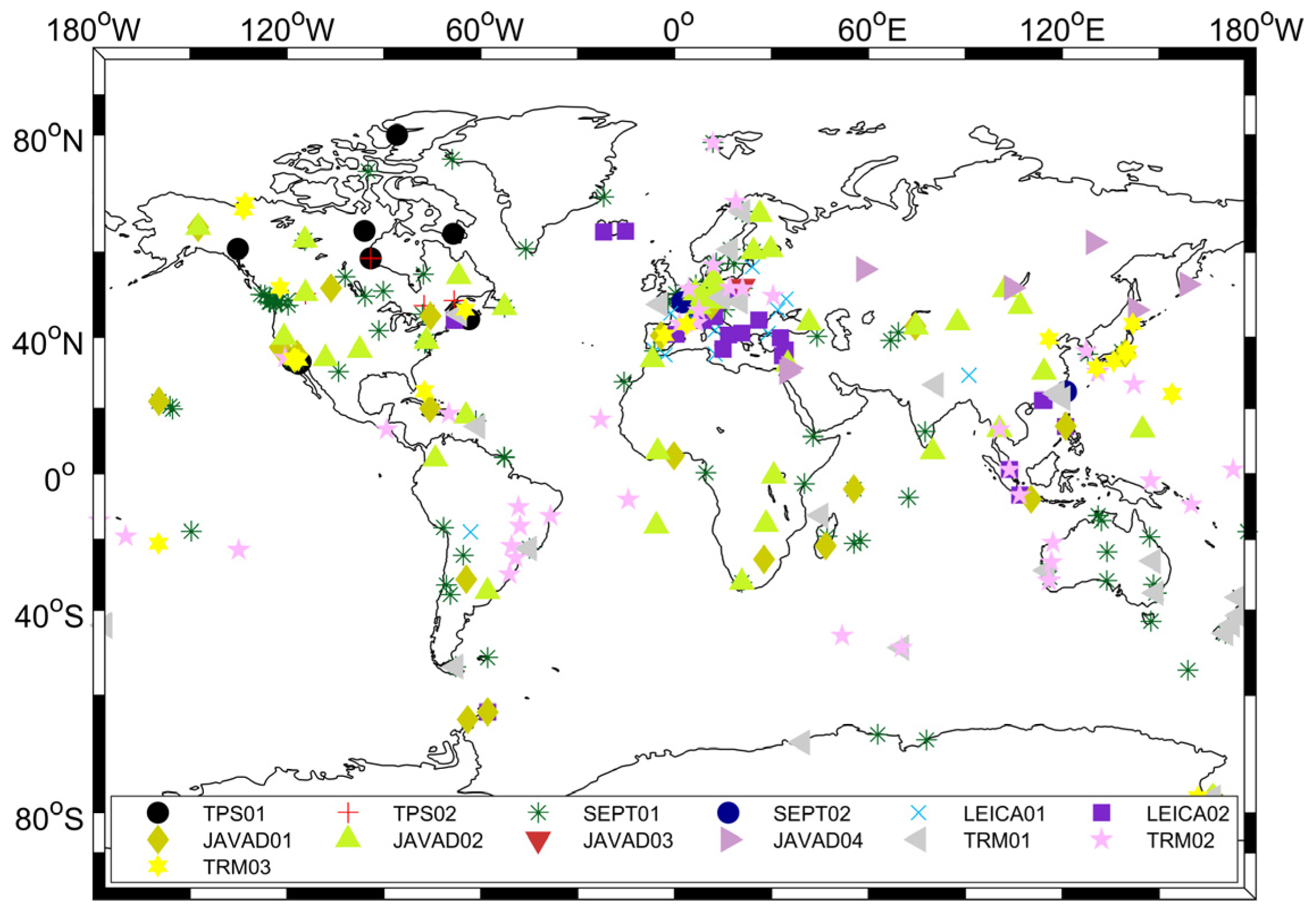
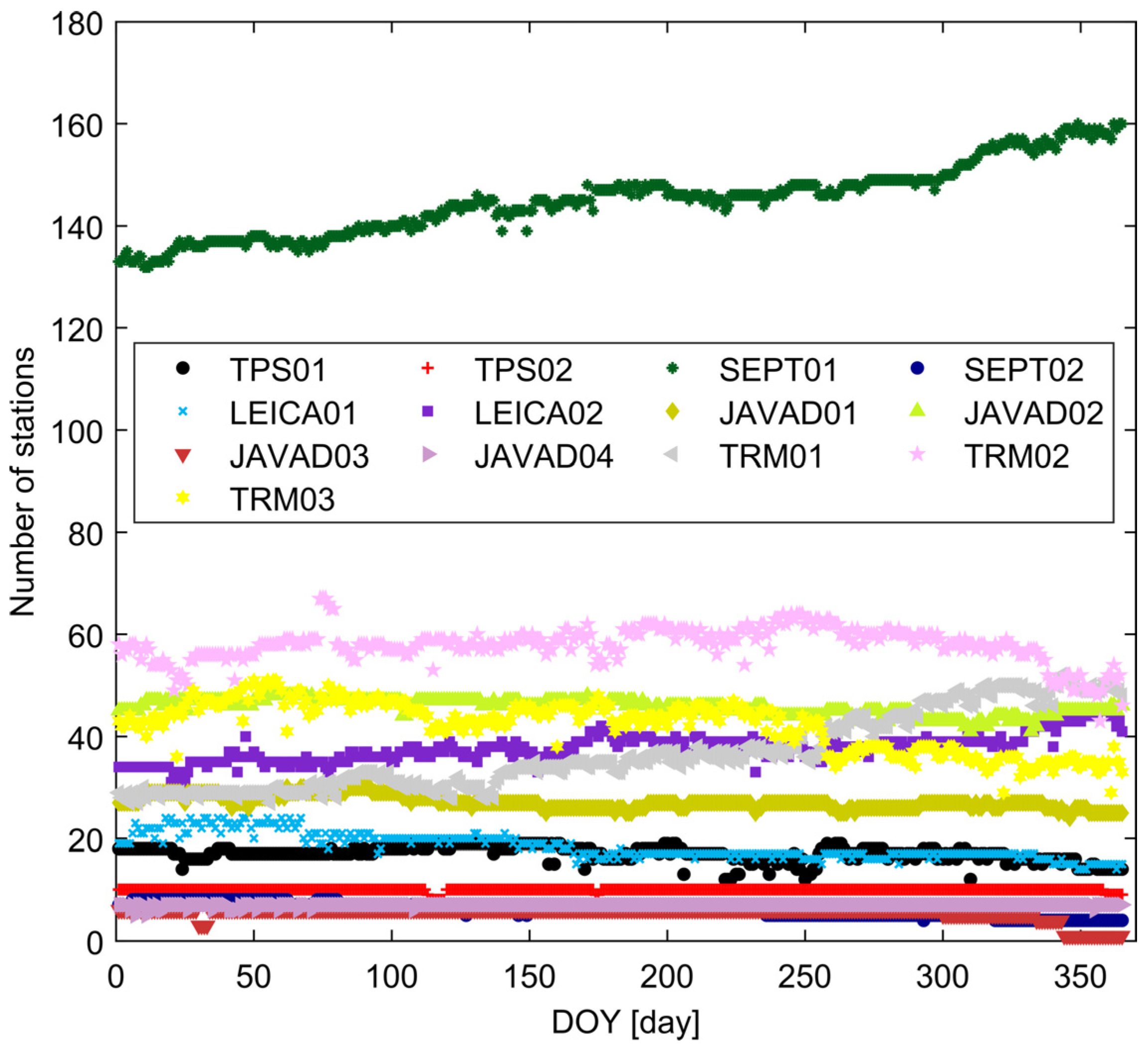
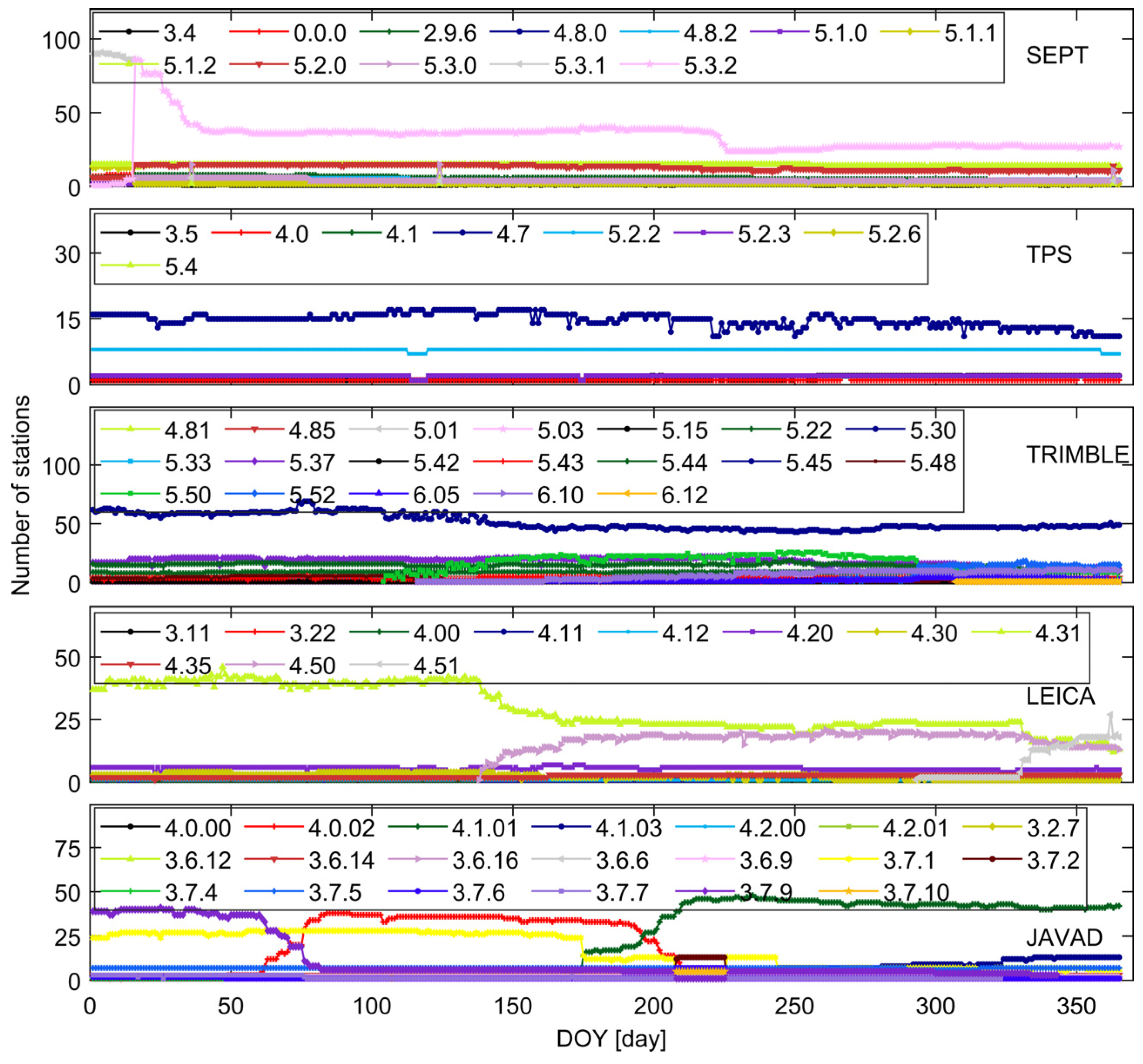
2.4. Data and Flowchart of Both Methods

Data from about 430 IGS stations are used to estimate the SDBs from DOY 1 to 365 in the year of 2021. Figure 1 illustrates the distribution of IGS stations on DOY 31, 2021. All these measurements are obtained from the following website: https://cddis.nasa.gov/archive/ (accessed on 20 November 2023). The assumption is that receivers with the same brand and model have equal SDB, so all receivers are classified into several groups according to the receiver model and brand. With the exception of some stations provided with brands TRIMBLE and JAVAD, they are classified according to the receiver brand and the firmware.

Table 1. Receiver grouping according to receiver types and models.

Group Name	Receiver Brand	Receiver Model
TPS01	TPS	NET-G3A
TPS02		NET-G5
SEPT01	SEPT	POLARX5TR/POLARX5/ASTERX4
SEPT02		POLARX4TR/POLARX4
LEICA01	LEICA	GR25/GR10
LEICA02		GR50/GR30
JAVAD01	JAVAD	TRE_G3TH DELTA/TR_G3TH/TRE_G2T DELTA
JAVAD02		TRE_3N DELTA/TRE_3 DELTA/TRE_3
JAVAD03		TRE_G3T DELTA
JAVAD04 *		-
TRM01	TRIMBLE	ALLOY
TRM02		NETR9
TRM03 *		-

* Groups marked with a star depend on the receiver model and version number.

illustrates the details of the classification of receiver groups. Figure 2 illustrates the updates in firmware versions across receivers from various brands. Each receiver brand includes a wide range of firmware versions. Notably, TRIMBLE receivers offer a total of 19 distinct firmware versions, while JAVAD receivers provide an even larger selection, with 20 different firmware versions available. Significant updates include the transition to 5.3.2 for SEPT receivers and 4.1.01 for LEICA receivers. Figure 3 presents the total number of receivers for all receiver groups in the IGS network. The number of SEPT01 receivers increased from 132 to 160 by the end of 2021, while the number of JAVAD03 receivers decreased from 6 to 2. The number of receivers in the remaining groups remained stable throughout the year.

The flowchart in Figure 4a outlines the methodology for estimating SDBs using the geometry-fixed/geometry-free method, which consists of three key stages. In the first stage, the process begins with input and initial processing, utilizing observation data, precise satellite orbit and clock corrections, antenna-phase center offsets, and ocean loading parameters, alongside a configuration file. In this stage, Precise Point Positioning (PPP) is performed using Ionospheric-Free (IF) code and phase linear combinations with fixed positions, producing a residual file with IF residuals, Melbourne–Wübbena wide-lane (MWWL) values, and Geometry-Free Ionospheric-Free (GFIF) values for each epoch, as described in Equation (2). The second stage focuses on calculating daily average bias. Daily averages of the IF and GFIF biases are computed through weighted averages to mitigate multipath and noise effects, while wide-lane (WL) ambiguity is rounded, and the weighted average of the MWWL bias is calculated, as outlined in Equation (3). These daily average biases are then transformed into biases (x, y, z), and the receiver group is determined based on the receiver classification. The final stage involves a least-squares adjustment with additional constraints to estimate the SDBs. This includes constructing the design matrix (B) and the observed-minus-computed vector (L), adding necessary conditions and executing the adjustment to generate the SDB file.

Similarly, Figure 4b illustrates the geometry-free method for SDB estimation, structured in three stages. The initial stage uses observation data, differential code biases (DCBs), and global ionospheric maps with a configuration file to calculate geometry-free (GF) linear combinations. This results in a residual file containing GF residuals, MWWL values, and GFIF values for each epoch, as shown in Equation (5). In the daily average bias calculation stage, daily averages for the GF and GFIF biases are determined using weighted averaging to address multipath and noise impacts, while WL ambiguity is rounded, and the daily weighted average of the MWWL bias is calculated, as detailed in Equation (6). Using Equation (7), these averages are transformed into biases (x, y, z), followed by receiver classification. The final stage involves SDB estimation through a least-squares adjustment with constraints. This includes constructing the design matrix (B), forming the vector (L), adding necessary conditions, and executing the adjustment to produce the SDB file.

Table 2. Processing parameters for SDB estimation using geometry-fixed/geometry-free method.

Items	Models
Observations	IF observables, MWWL observables, and GFIF observables
Interval	30 s
Elevation cutoff angle	15°
Ionospheric effect	IF observables are utilized to mitigate the first-order ionospheric effect
Troposphere delay	The dry tropospheric delay is modeled, while the wet tropospheric delay is estimated as an unknown
Phase center offset and variations	Igs14.atx
Weighting scheme	Elevation-based is used

illustrates the processing parameters of the geometry-fixed/geometry-free method, while

Table 3. Processing parameters for SDB estimation using geometry-free method.

Items	Models
Observations	GF observables, MWWL observables, and GFIF observables
Interval	30 s
Elevation cutoff angle	15°
Ionospheric effect	Mitigated by using final global ionospheric maps
Satellite and receiver DCB	Estimated by MDCB MATLAB code
Weighting scheme	Elevation-based is used

presents the parameters for the geometry-free method.

3. Results

This section compares the SDB estimates derived from the two methods and assesses their validity through a statistical analysis of short-term and long-term stability. Figure 5 presents weekly SDB values for the C1C signal of GPS satellite G01 in 2021, calculated using both geometry-free and hybrid methods. Weekly C1C SDB values are used instead of daily values to mitigate high noise levels observed in daily SDBs. The annual C1C SDBs can be calculated as the average of C1C SDBs throughout the year. For receiver groups TPS01, SEPT02, LEICA01, and JAVAD04, the difference between the annual SDBs of GPS satellite G01 for both methods is greater than 0.10 ns. For the remaining receiver groups, the difference between the annual C1C SDBs of GPS satellite G01 for both methods is below 0.05 ns. This indicates that using the dual-frequency GF linear combination rather than the dual-frequency IF linear combination produces significantly different SDB estimates. From the perspective of stability analysis, the weekly C1C SDBs for satellite G01 for all receiver groups demonstrate a comparable level of stability between the two methods with an overall STD less of 0.10 ns. Figure 6 displays the C2W SDB values of GPS satellite G01 in 2021, obtained through both methods. For receiver groups TPS01, LEICA01, LEICA02, and JAVAD04, the annual SDB differences between the two methods are approximately 0.15 ns. In contrast, for the remaining receiver groups, the annual C2W SDB differences are below 0.05 ns. Statistically, the weekly C2W SDBs for satellite G01 for all receiver groups exhibit similar stability between the two methods, with an overall STD below 0.10 ns.

Figure 7 illustrates the annual SDB differences between the two methods for signals C1C and C2W, for thirteen receiver groups, as well as the overall annual SDB difference for all satellites. The overall annual SDB differences between the two methods range from 0.05 ns to 0.11 ns. This finding highlights that applying the GF linear combination instead of the IF linear combination results in systematic SDB differences across all satellites and receiver groups. For all receiver groups, the annual SDB differences between the two methods remain substantial, regardless of the number of receivers in each group. Notably, receiver groups such as TRM03, TRM02, JAVAD01, and SEPT01, which include a large number of receivers, still exhibit notable differences in annual SDB values for certain satellites. These results demonstrate that the performance of the proposed method relies on the use of GF linear combinations and remains unaffected by the number of receivers within a group.

To evaluate the long-term stability of SDBs, the yearly STD is computed for each satellite and receiver group over the entire year. Figure 8 presents the yearly STD of C1C SDBs for each satellite across all receiver groups, as well as the overall yearly STD for all satellites. For receiver groups SEPT01, TRM02, and TRM03, the yearly STDs of C1C SDBs for all satellites show similar stability, with STDs of less than 0.1 ns for both methods. For the remaining receiver groups, yearly STDs of C1C SDBs are less than 0.25 ns, except for GPS satellite G24 in group SEPT02, for both methods. The overall yearly STDs for all satellites for both methods are consistent. As a result, the weekly C1C SDBs for all receiver groups demonstrate a comparable level of stability between the two methods with an overall STD of less than 0.10 ns. Figure 9 presents the yearly STD of C2W SDBs for each satellite across all receiver groups, along with the overall yearly STD for all satellites. For all receiver groups except for receiver group LEICA02, the C2W SDBs of the geometry-free method demonstrate better stability compared to those of the hybrid method. Particularly for groups SEPT01, TRM02, and TRM03, which have a large number of receivers, the geometry-free method shows better stability. Similarly, the overall yearly standard deviation (STD) for all satellites remains consistent, and the weekly C2W SDBs across all receiver groups exhibit similar stability between the two methods, with an overall STD of less than 0.10 ns. Long-term stability is influenced by two primary factors: (1) the number of receivers within each group and (2) the precision of residuals derived from the applied linear combinations. Receiver groups such as SEPT01, TRM03, TRM02, and JAVAD01 exhibit similar stability characteristics due to their large number of receivers, which reduces the impact of the precision of linear combinations on stability. An increase in the number of receivers within a group generally enhances long-term stability. In contrast, when the number of receivers within a group is limited, the precision of the applied linear combinations has a greater influence on long-term stability.

For the short-term stability of SDB, the weekly STD is computed for each satellite and receiver group for 7-day SDBs throughout the entire year. Figure 10 and Figure 11 illustrate the distribution of weekly STDs for GPS C1C SDB and GPS C2W SDB, respectively, using both methods. In Figure 9, 91% and 95.4% of C1C SDB STDs are within 0.1 ns for the geometry-free and hybrid methods, respectively. In Figure 10, 89% and 91% of C2W SDB STDs are within 0.1 ns for the geometry-free and hybrid methods, respectively. As a conclusion, both method are statistically consistent for the short- and long-term stability.

4. Discussion

SDBs have a significant impact on both satellite and receiver DCB estimation. Ignoring SDBs in DCB estimation leads to their incorporation into both satellite and receiver DCBs, especially when using a network of receivers from the same group. The mean of satellite SDBs is assimilated by the receiver DCB, while the remaining portions are absorbed by satellite DCBs, causing inconsistencies in satellite DCB estimates across different receiver groups. Thus, the satellite DCB estimation is affected by a GF combination of SDBs from each group, with their impact calculated proportionally according to the number of receivers in each group.

With observation data from 1 January 2021 to 30 January 2021, satellite DCB estimation was used to validate the accuracy of estimated SDBs using both geometry-free and geometry-free/geometry-fixed methods across different receiver groups. Satellite DCBs were estimated individually for each group and collectively for all receivers. Figure 12 illustrates the estimates of DCB for GPS satellite G06 from thirteen receiver groups, under three different scenarios: geometry-free SDBs, geometry-fixed/geometry-free SDBs, and no-correction SDBs. In the geometry-free SDBs, the satellite DCBs for all receiver groups exhibit relative stability around −7.7 ns, with minor variations during the experimental duration. This stability indicates that the geometry-free approach effectively mitigates the influence of SDBs on the satellite DCB estimates. In contrast, the geometry-fixed/geometry-free SDBs exhibit greater variability. The no-correction SDBs show the highest variability and deviation from the mean satellite DCB, with estimates ranging from approximately −6.2 ns to −8.3 ns. This significant spread indicates that without any correction, the DCB estimates are highly affected by SDBs.

Figure 13 illustrates the average bias in satellite DCBs for various receiver groups under the three different scenarios: geometry-free SDBs, geometry-fixed/geometry-free SDBs, and no correction. The average bias in satellite DCB equals the difference between the satellite DCB estimated with receivers from the same group and the satellite DCB estimated with all receivers. The geometry-free SDBs demonstrate the lowest average bias across all receiver groups, assuring the accuracy and validity of the geometry-free SDBs in DCB estimation for all receiver groups. With geometry-free SDBs, the average bias is below 0.15 ns, and an STD is 0.10 ns. The geometry-fixed/geometry-free SDBs exhibit an increased mean bias compared to the geometry-free SDBs scenario. With geometry-fixed/geometry-free SDBs, the average bias is below 0.20 ns, and an STD is 0.16 ns. The no-correction scenario shows the highest mean bias for all receiver groups. Figure 14 compares the distribution of DCB residuals for two different scenarios: geometry-free SDBs and geometry-fixed/geometry-free SDBs. The geometry-free SDBs show a distribution of residuals that are generally small and closely clustered with an STD of 0.10 ns. This suggests that the geometry-free approach effectively minimizes residual biases, leading to more accurate DCB estimates. In contrast, the geometry-fixed/geometry-free SDBs follow a wider distribution of residuals with an STD of 0.16 ns. Overall, the comparison highlights the superior performance of the geometry-free SDBs in achieving lower and more consistent DCB estimates.

5. Conclusions

Signal distortion bias (SDB) in GNSS data processing leads to systematic bias in pseudoranges, which affects the DCB estimation. The stability of SDBs, allowing them to be treated as constant values, highlights the importance of investigating both their stability and accuracy. In our study, we propose using three geometry-free linear combinations, namely the dual-frequency geometry-free linear combination, the MWWL linear combination, and the triple-frequency GFIF linear combination. This approach aims to improve the stability and accuracy of SDBs by demonstrating consistency in the residuals obtained from these combinations.

Data from nearly 450 receivers from 1 January to 31 December 2021 were used to examine the estimation accuracy and short-term and long-term stability of GPS C1C SDBs and C2W SDBs using two methods: (1) the hybrid method and (2) the geometry-free method. The first method, the hybrid method, incorporates three linear combinations: one dual-frequency IF observable with fixed receiver positions, and two geometry-free linear combinations, namely the MWWL linear combination and the GFIF linear combination. The second method, the geometry-free method, employs three GF linear combinations: the dual-frequency GF linear combination, the MWWL observable, and the GFIF observable. Yearly and weekly STDs were calculated to assess the statistical stability of GPS C1C and C2W SDBs. The results demonstrate that both methods achieve comparable short- and long-term stability across most receiver groups and satellites. Specifically, for long-term stability, the yearly STDs of GPS C1C SDBs for both methods are consistent, with overall values below 0.1 ns for most receiver groups. Short-term stability, assessed through weekly STDs, reveals that 91% and 95.4% of GPS C1C SDB STDs are within 0.1 ns for the geometry-free and hybrid methods, respectively, while for GPS C2W SDBs, 89% and 91% of weekly STDs fall within this range for the geometry-free and hybrid methods, respectively. These results indicate that both methods are statistically robust in terms of short-term stability. SDB estimation and stability are influenced by the number of receivers within a group and the accuracy of residuals derived from the linear combinations. Groups with a larger number of receivers, such as SEPT01, TRM02, TRM03, and JAVAD01, benefit from the averaging effect of multiple receivers, reducing the impact of linear combination accuracy. Conversely, for smaller receiver groups, the accuracy of linear combinations plays a more significant role in SDB estimation.

SDBs have a significant impact on both satellite and receiver DCB estimation. With observation data from 1 January 2021 to 30 January 2021, satellite DCB estimation was used to validate the accuracy of estimated SDBs using both geometry-free and hybrid methods across different receiver groups. Satellite DCBs were estimated individually for each group and collectively for all receivers. The results demonstrate that geometry-free SDBs provide stable satellite DCB estimates, with an average bias below 0.15 ns. This stability indicates that the geometry-free approach effectively mitigates the influence of SDBs. In contrast, hybrid SDBs exhibit greater variability and higher mean bias, with an average bias below 0.20 ns. The no-correction scenario shows the highest mean bias across all receiver groups. The geometry-free SDBs also display a tightly clustered distribution of residuals, with a zero mean and an STD of 0.10 ns, suggesting minimal residual biases and more accurate DCB estimates. Overall, the comparison underscores the superior performance of geometry-free SDBs in achieving lower and more consistent DCB estimates.

References

1. Phelts, R.E.; Akos, D.M.; Enge, P. Robust signal quality monitoring and detection of evil waveforms. In Proceedings of the 13th International Technical Meeting of the Satellite Division of The Institute of Navigation (ION GPS 2000), Salt Lake City, UT, USA, 19–22 September 2000. [Google Scholar]
2. Pini, M.; Akos, D.M.; Esterhuizen, S.; Mitelman, A. Analysis of GNSS signals as observed via a high gain parabolic antenna. In Proceedings of the 18th International Technical Meeting of the Satellite Division of The Institute of Navigation (ION GNSS 2005), Long Beach, CA, USA, 13–16 September 2005. [Google Scholar]
3. Hauschild, A.; Montenbruck, O. A study on the dependency of GNSS pseudorange biases on correlator spacing. GPS Solut. 2014, 20, 159–171. [Google Scholar] [CrossRef]
4. Mi, X.; Sheng, C.; El-Mowafy, A.; Zhang, B. Characteristics of receiver-related biases between BDS-3 and BDS-2 for five frequencies including inter-system biases, differential code biases, and differential phase biases. GPS Solut. 2021, 25, 113. [Google Scholar] [CrossRef]
5. Gong, X.; Zheng, F.; Gu, S.; Zhang, Z.; Lou, Y. The long-term characteristics of GNSS signal distortion biases and their empirical corrections. GPS Solut. 2022, 26, 52. [Google Scholar] [CrossRef]
6. Lou, Y.; Zhang, Z.; Gong, X.; Zheng, F.; Gu, S.; Shi, C. Estimating GPS satellite and receiver differential code bias based on signal distortion bias calibration. GPS Solut. 2023, 27, 48. [Google Scholar] [CrossRef]
7. Montenbruck, O.; Hauschild, A.; Steigenberger, P. Differential code bias estimation using multi-GNSS observations and global ionosphere maps. Navig. J. Inst. Navig. 2014, 61, 191–201. [Google Scholar] [CrossRef]
8. Hauschild, A.; Steigenberger, P.; Montenbruck, O. Inter-receiver GNSS pseudorange biases and their effect on clock and DCB estimation. In Proceedings of the 32nd International Technical Meeting of the Satellite Division of The Institute of Navigation (ION GNSS+ 2019), Miami, FL, USA, 16–20 September 2019. [Google Scholar]
9. Cui, B.; Li, P.; Wang, J.; Ge, M.; Schuh, H. Calibrating receiver-type-dependent wide-lane uncalibrated phase delay biases for PPP integer ambiguity resolution. J. Geod. 2021, 95, 82. [Google Scholar] [CrossRef]
10. Gong, X.; Lou, Y.; Zheng, F.; Gu, S.; Shi, C.; Liu, J.; Jing, G. Evaluation and calibration of BeiDou receiver-related pseudorange biases. GPS Solut. 2018, 22, 98. [Google Scholar] [CrossRef]
11. Zhang, Y.; Kubo, N.; Chen, J.; Wang, A. Calibration and analysis of BDS receiver-dependent code biases. J. Geod. 2021, 95, 1–14. [Google Scholar] [CrossRef]
12. Zheng, F.; Gong, X.; Lou, Y.; Gu, S.; Jing, G.; Shi, C. Calibration of BeiDou triple-frequency receiver-related pseudorange biases and their application in BDS precise positioning and ambiguity resolution. Sensors 2019, 19, 3500. [Google Scholar] [CrossRef] [PubMed]
13. Montenbruck, O.; Steigenberger, P.; Prange, L.; Deng, Z.; Zhao, Q.; Perosanz, F.; Romero, I.; Noll, C.; Stürze, A.; Weber, G.; et al. The Multi-GNSS Experiment (MGEX) of the International GNSS Service (IGS)–achievements, prospects and challenges. Adv. Space Res. 2017, 59, 1671–1697. [Google Scholar] [CrossRef]
Figure 1. Distribution of the IGS stations on 31 January 2021.
Remotesensing 16 04463 g001
Figure 2. Number of receivers for different receiver groups in 2021.
Remotesensing 16 04463 g002
Figure 3. Distribution of firmware versions across stations in 2021.
Remotesensing 16 04463 g003
Figure 4. Flowchart of the source code for SDB estimation using the two methods: (a) the hybrid method and (b) the geometry-free method.
Remotesensing 16 04463 g004
Figure 5. SDB weekly means of GPS signal C1C for satellite G01 in 2021.
Remotesensing 16 04463 g005
Figure 6. SDB weekly means of GPS signal C2W for satellite G01 in 2021.
Remotesensing 16 04463 g006
Figure 7. Annual difference between estimated SDBs for the two methods: SDB C1C (cyan); SDB C2W (blue).
Remotesensing 16 04463 g007
Figure 8. Annual STDs of C1C SDBs for all receiver groups in 2021.
Remotesensing 16 04463 g008
Figure 9. Annual STDs of C2W SDBs for all receiver groups in 2021.
Remotesensing 16 04463 g009
Figure 10. Weekly STDs of C1C SDBs for all receiver groups in 2021.
Remotesensing 16 04463 g010
Figure 11. Weekly STDs of C2W SDB for all receiver groups in 2021.
Remotesensing 16 04463 g011
Figure 12. DCB estimates for GPS satellite G06 from 13 receiver groups, under three different scenarios: geometry-free SDBs, geometry-fixed/geometry-free SDBs, and no-correction SDBs.
Remotesensing 16 04463 g012
Figure 13. Mean bias in satellite DCBs for various receiver groups under the three different scenarios: geometry-free SDBs, geometry-fixed/geometry-free SDBs, and no correction.
Remotesensing 16 04463 g013
Figure 14. Distribution of biases in satellite DCB for two different scenarios: geometry-free SDBs and geometry-fixed/geometry-free SDBs.
Remotesensing 16 04463 g014