Abstract
High-precision monitoring of glacier motion provides crucial information for a thorough understanding of the dynamic characteristics and development patterns of glaciers, which serves as a scientific basis for the prevention and management of glacier-related disasters. Zelongnong Glacier, located in Tibet, China, has experienced glacier surges, collapse, and hazard chains four times in the last 70 years. On 10 September 2020, a major glacier hazard chain occurred in this region. To reveal the influencing factors of the glacier motion, we monitor the Zelongnong Glacier motions with 65 scenes of TerraSAR/PAZ images from 2022 to 2023, where the Pixel Offset Multidimensional Small Baseline Subset (PO-MSBAS) method is employed for three-dimensional time series inversion. As the registration window size directly affects the matching success rate, deformation accuracy, and signal-to-noise ratio (SNR) during the offset tracking processing, we adopt a variable window-weighted cross-correlation strategy. The strategy balances the advantages of different window sizes, effectively reducing noise while preserving certain details in the offset results. The standard deviation in stable areas is also significantly lower than that obtained using smaller window sizes in conventional methods. The results reveal that the velocity of the southern glacier tributary was larger than the one in the northern tributary. Specifically, the maximum velocity in the northern tributary reached 45.07 m/year in the horizontal direction and −7.45 m/year in the vertical direction, whereas in the southern tributary, the maximum velocity was 50.15 m/year horizontally and 50.66 m/year vertically. The southern tributary underwent two bends before merging with the mainstream, leading to a more complex motion pattern. Lastly, correlation reveals that the Zelongnong Glacier was affected by the combined influence of temperature and precipitation with a common period of around 90 days.
1. Introduction
In the context of global climate warming, glaciers around the world are undergoing accelerated melting, which has intensified the frequency of glacier-related natural disasters [1]. The glaciers and the moraines in their vicinity exhibit substantial size and extensive spread. Disasters such as glacier debris flows, glacier lake outburst floods, and landslides caused by glacier movement can be highly destructive [2]. Therefore, the study of the dynamic evolution of glaciers and their associated characteristics is crucial for understanding how glaciers respond to climate change and for predicting glacier-related natural disasters [3]. Compared with optical remote sensing images, synthetic aperture radar (SAR), as an active microwave sensor, can work under day and night and all weather conditions, demonstrating significant potential in monitoring glacier velocities in mountainous regions [4].
The Pixel Offset Tracking (POT) technique, based on SAR intensity information, is a dominant method for estimating two-dimensional surface deformation from SAR images. It can obtain glacier motion over long time intervals once the surface features can be maintained [5]. Cai et al. proposed a Polarimetric SAR pixel offset tracking method (PCM-POT) to alleviate the dependence of offset estimation on the matching window size in response to the inherent trade-off between matching accuracy and detailed information preservation in SAR POT methods by using the single polarization intensity [6]. To address the impact of scattering noise and strong point scattering on offset estimation accuracy, Du et al. utilized a sensor- and scene-independent threshold to filter out high-amplitude pixels [7]. A correlation stacking method was developed by Li et al., which effectively reduces the noise floor in normalized cross-correlation (NCC), enhancing both spatial resolution in offset tracking and velocity field coverage [8]. Meanwhile, Yang et al. proposed a method to estimate three-dimensional surface displacement using offset tracking with single amplitude pair (SAP) SAR data, effectively easing the stringent data requirements of traditional methods [9].
However, the accuracy and temporal resolution of the two-dimensional velocities are limited [10]. To reveal the glacier’s actual motion characteristics, it is widely applied to integrate offset tracking results from ascending and descending SAR images to derive the three-dimensional time series using the Small Baseline Subset (SBAS) or Multidimensional Small Baseline Subset (MSBAS) methods. Shi et al. estimated the three-dimensional time series of glacier movements using the improved PO-SBAS method with Sentinel-1A ascending and descending SAR images acquired from 2017 to 2018 [11]. Yang et al. used the PO-SBAS method to derive the three-dimensional motion fields of glaciers terminating in lakes and those terminating on land and analyzed the different spatiotemporal characteristics [12]. Guo et al. improved the PO-MSBAS method and obtained the three-dimensional velocity time series of the Hispar Glacier during its surge period based on Sentinel-1 images, revealing the triggering mechanisms of the glacier surge [10].
The temperature on the Tibetan Plateau has risen significantly, with the rate of increase being twice the global average value over the past two decades [13,14]. The high mountain valleys of southeastern Tibet, particularly in the Yarlung Tsangpo region, develop numerous maritime glaciers that are more sensitive to monsoon climate and temperature changes, leading to a higher rate of glacier mass loss [15,16]. For example, Zelongnong Glacier experienced glacier surges in 1950 and 1968 [17]. Given the rising temperatures and the frequent occurrence of geological hazards in recent years, the glacier’s motion is of significant concern. We used the PO-MSBAS method to ascend and descend TerraSAR/PAZ images to obtain the glacier’s velocity, analyze the spatiotemporal characteristics of surface motion, and investigate the correlation between glacier motion and precipitation and temperature, so as to gain an in-depth understanding of glacier dynamic characteristics and development patterns to provide scientific reference for monitoring and predicting glacier movement as well as for the prevention and management of the glacier-related disasters.
2. Study Area and Datasets
2.1. Study Area
The Zelongnong valley (29.58972 to 29.66416N, 94.94306 to 95.05528E) is situated in Paizhen, Milin County, Linzhi City, Tibet, China, at the entrance of the Yarlung Tsangpo Grand Canyon shown in Figure 1. The area of the valley is about 53.04 km2, the length of the main valley is approximately 12.18 km, the elevation ranges from 2847 m to 7782 m, and the average decrease in slope is 274‰. The glacier is a typical glacier developed near the Namcha Barwa Peak, which is one of the largest modern glaciers in this region. The glacier mainly consists of two tributaries from the north and south covering at 4100 m that form the main stream in a “Y” shape, occupying an area of about 7.63 km2. The snout of the glacier is located at 29.616N, 94.988E. The warm and humid air from the Indian Ocean brings a substantial amount of rainfall which, together with the influence of the cliff terrain and very high altitude, results in abundant ice and snow melt water and intense glacier activity.
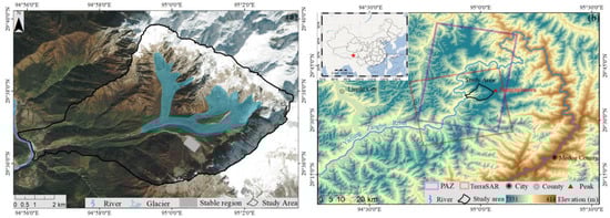
Figure 1.
Geographical location of the study area. (a) Optical image of Zelongnong Glacier, with the Snout Located at 29.616N, 94.988E. (b) The location of Zelongnong valley and the coverage of the SAR datasets.
2.2. Datasets
In this study, 65 scenes of TerraSAR/PAZ images (including 28 ascending and 37 descending images) were collected as shown in Figure 1a, where the line-of-sight (LOS) and azimuth pixel spacing are higher than 3 m, and the detailed parameters are given in Table 1. As for the offset tracking processing, 99 pairs of high-quality offset combination pairs for ascending orbits and 69 pairs of high-quality offset combination pairs for descending orbits were obtained as shown in Figure 2.

Table 1.
The main parameters of the SAR datasets.
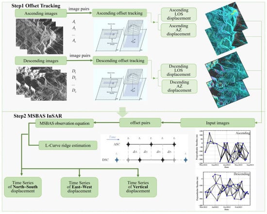
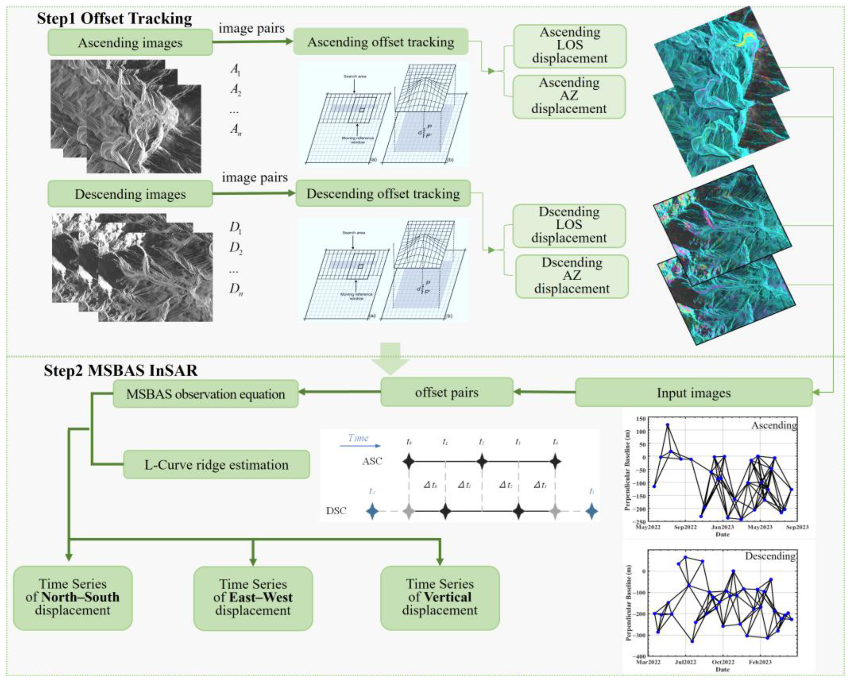
Figure 2.
Block diagram of the PO-MSBAS method.
In addition, the SRTM DEM, with a resolution of 30 m, was used in this study for geographic alignment and to calculate the local SAR image incidence and azimuth angles. The precipitation data (GPM, https://gpm.nasa.gov (accessed on 22 September 2024)) and daily mean temperature data (ERA5, https://cds.climate.copernicus.eu/ (accessed on 22 September 2024)) for the corresponding time periods, both with a resolution of 0.1° × 0.1°, were analyzed to assess their influences on glacial movement.
3. Methodology
Figure 1 shows the block diagram of calculating the three-dimensional time series of glacier movement with the PO-MSBAS method. The process can be divided into two main steps: Step 1, offset tracking to obtain the LOS and azimuth movements from the ascending and descending SAR images, and Step 2, the MSBAS method for deriving the three-dimensional time series.
3.1. Offset Tracking with Variable Window-Weighted Cross-Correlation
The main steps to obtain the LOS and azimuth deformation using the offset tracking method include precise SAR image registration, offset calculation, and converting the separated real and imaginary parts of the results into LOS and azimuth components [12,18,19]. The selection of the registration window is the critical part, as the window size directly affects the matching success rate, the accuracy of the deformation results, and the signal-to-noise ratio [20,21]. The basic principle of offset calculation using a fixed registration window size is to determine the offset by calculating the position of the peak cross-correlation coefficient between the fixed window in the reference image and in the search image [20,22,23]. The cross-correlation coefficient can be expressed as follows:
where m and n are the matching window size; M and S denote the intensity of SAR image pixels in the matching windows of the master and slave images, respectively; and represent the average intensity of SAR images in the matching windows of the master and slave images; and p denotes the correlation coefficient. The closer p is to 1, the higher the correlation between the master and slave images.
In order to improve the accuracy of offset estimation, Liu et al. proposed an improved offset tracking algorithm, which obtains a series of offset estimation sets by adjusting different image window sizes of the image block, so that each element in the estimated offset set is reordered by magnitude and the median element is taken as the final offset estimation for pixel i [24]. While retaining the median value improves the robustness of the method, it also results in the loss of effective information obtained from other registration window sizes. Therefore, we propose an offset tracking method based on variable window-weighted cross-correlation. After obtaining a series of offset estimation sets , the maximum cross-correlation coefficients within different window sizes are calculated. Then, the weight is determined for each window size, and the final offset can be estimated as follows:
The new improved method can integrate the advantages of different windows to reduce the noise and maintain certain details of the offset result. The principle of the weighted variable window cross-correlation calculation method is illustrated in Figure 3.
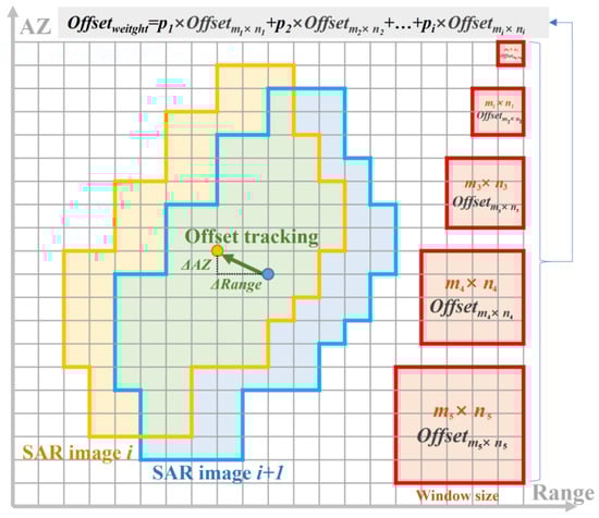
Figure 3.
The illustration of the offset tracking method based on variable window-weighted cross-correlation.
In this study, we set the minimum window size as 64 × 64 and the maximum window size as 256 × 256, with a window step size of 32 × 32 and a search step size of 5 × 5. Additionally, we set the correlation threshold to 0.2 to mask out unreliable results obtained from areas with low surface texture, shadows, and other regions.
3.2. MSBAS
The conventional MSBAS technique is applied to the interferometric stage observations to extract the two-dimensional or three-dimensional deformation rate of the ground surface [25,26,27]. For large-scale displacements, such as those from glaciers or landslides, which exceed the monitoring range of InSAR technology, the LOS and azimuthal results obtained from the offset tracking method can be used as input values for the MSBAS deformation model [12,21].
After obtaining the LOS and azimuth deformation from the ascending and descending data, respectively, inverting the three-dimensional deformation time series with MSBAS technology involves the construction of functional models between the deformation components in the east–west, north–south, and vertical directions and the imaging geometry parameters of the ascending and descending orbit SAR images, as shown in Equation (4):
where is the azimuth angle of the SAR images, is the look angle, and means the time interval between SAR images; , , represent the deformation velocities in the north, east, and vertical directions, respectively; , represent the LOS and azimuth deformation of the ascending SAR images; and , represent the LOS and azimuth deformation of the descending SAR images. So, Equation (4) can be further simplified as follows:
where A is the coefficient matrix, which is composed of the projection coefficients between three-dimensional deformation and azimuth and LOS directions and the time intervals of neighboring SAR images; X is the parameters to be solved; and L is the observation vector. When the coefficient matrix A is full rank, Equation (4) can be solved based on the least squares criteria. However, since SAR images from different tracks are acquired at different times, this causes more unknown parameters than equation numbers, resulting in a rank-deficient and underdetermined problem [28]. Therefore, the least squares method cannot provide unique and reliable estimations. To solve this problem, the regularization is considered, and the parameters can be estimated as follows:
where λ is the Tikhonov regularization factor and I is the identity matrix.
Next, the obtained three-dimensional deformation rates are integrated over the time intervals between two adjacent SAR image acquisitions to obtain the three-dimensional deformation time series as follows:
The parameters of glacier velocity and horizontal velocity are shown below:
3.3. Wavelet Cross-Transform (WXT)
Wavelet Transform (XT) is a commonly used time–domain analysis method that reveals the hierarchical and periodic characteristics of signals at different time scales [29]. To further investigate the relationship between glacier velocity and its influencing factors, this study will employ WXT for correlation analysis.
The WXT of the two time series can be represented as follows:
where denotes the complex conjugate of and represents the cross-wavelet power spectrum. The equation can be expressed as follows:
where represents the subwavelet, is the complex conjugate of the subwavelet, is the translation parameter, and is the scaling factor.
4. Results
4.1. Three-Dimensional Glacier Velocities Maps
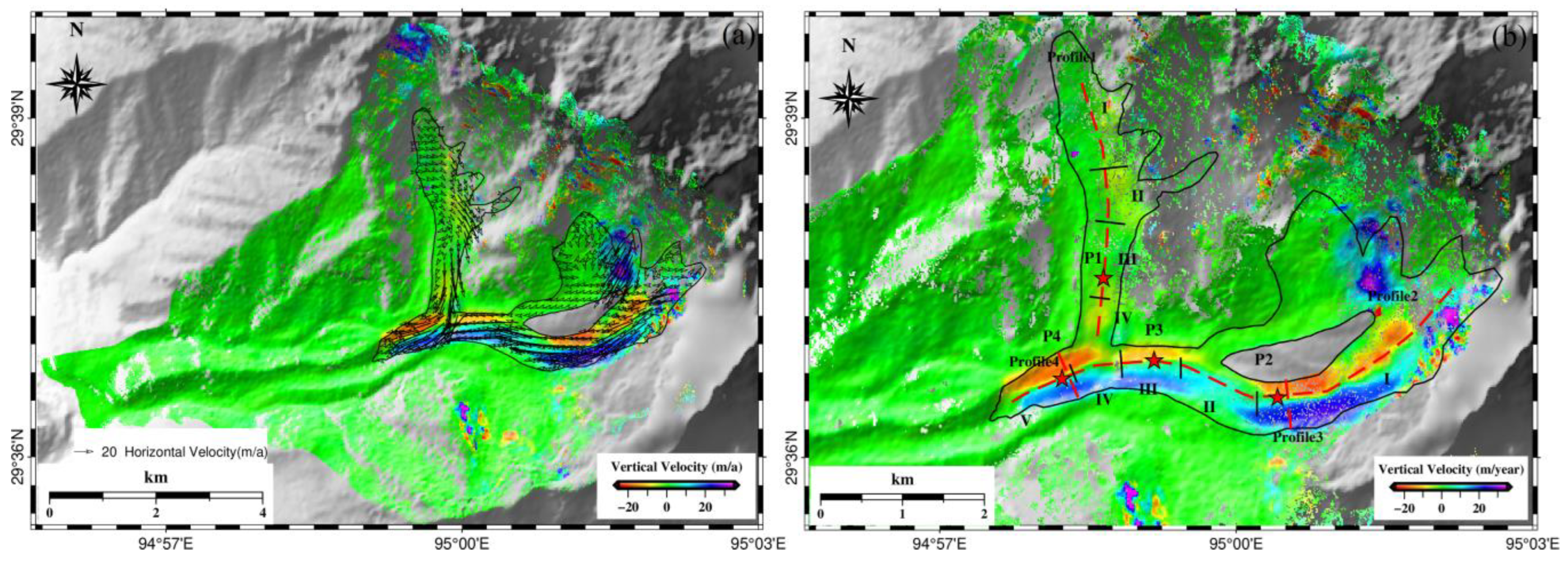
In this study, the PO-MSBAS technique was employed to derive the three-dimensional glacier motion velocities. Figure 4a shows the three-dimensional velocity map of Zelongnong Glacier from 22 June 2022 to 28 June 2023, where the horizontal velocity is shown by vectors; the vertical velocity is color-coded, with red indicating downward motion. To better analyze the spatial glacier motion characteristics, four profiles were selected along the glacier motion direction and the cross-section of the main stream in Figure 4b. The velocity profiles of the horizontal and vertical motions are plotted in Figure 5, where the error bars indicate the standard deviation calculated in the 3 × 3 pixels around the given pixel.
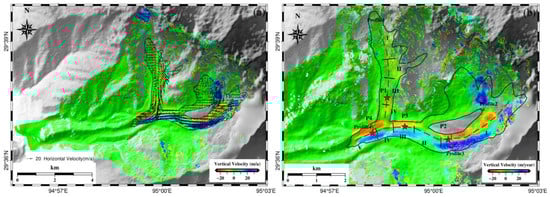
Figure 4.
Three-dimensional velocity maps of Zelongnong Glacier. (a) Three-dimensional glacier velocity map, where the horizontal velocities are shown in vectors, and the vertical velocities are color-coded; (b) distribution of four feature points and four profiles along with their stages on the vertical velocity map. The feature points P1–P4 are represented by red pentagrams, while the profiles 1–4 are shown as red line segments. The stages are indicated by I–V.
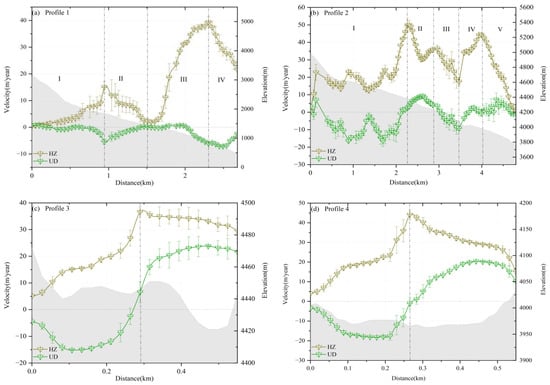
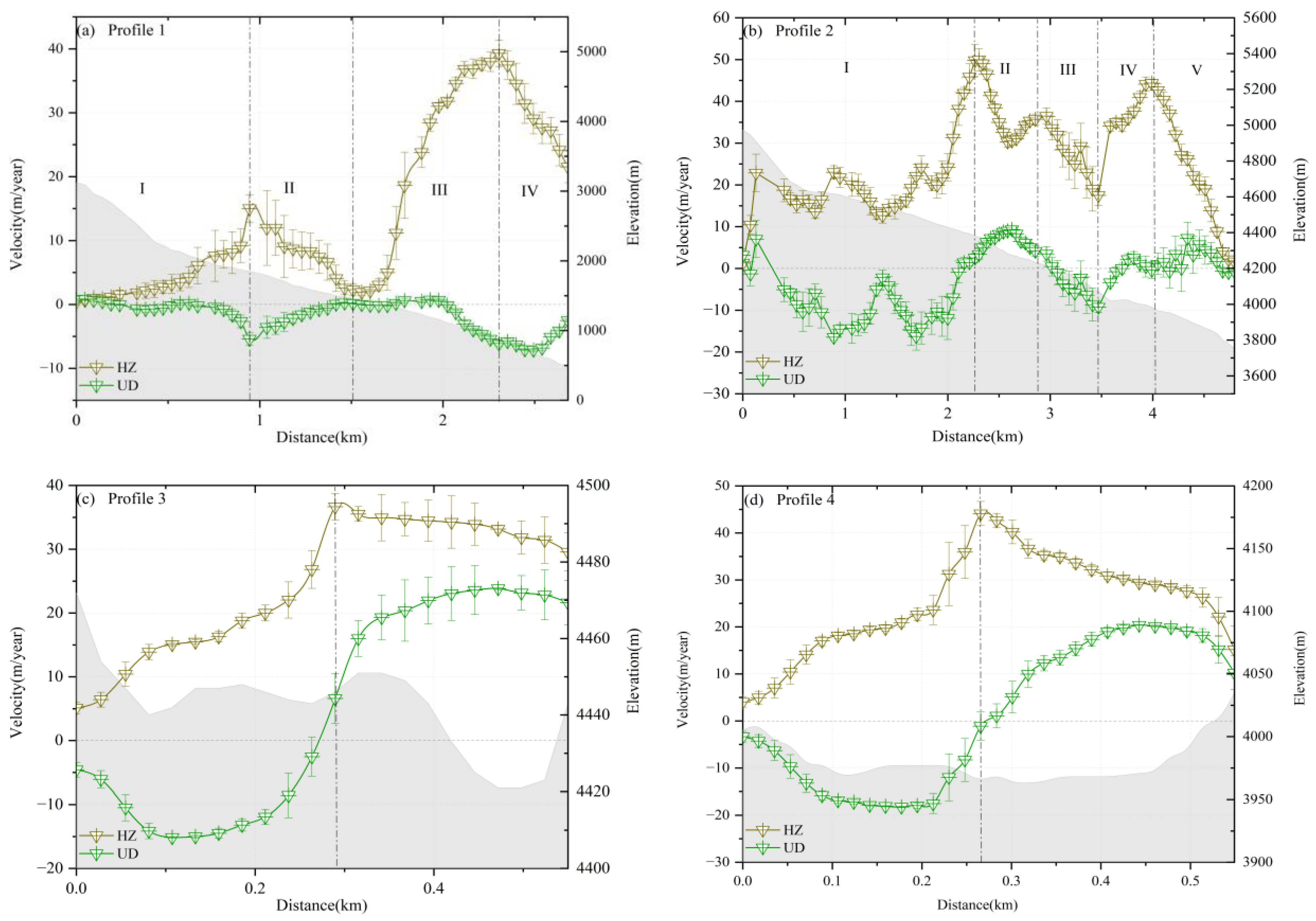
Figure 5.
Three-dimensional glacier velocity and elevation along the profile, where the error bars indicate the standard deviation within 3 × 3 pixels.
The spatiotemporal three-dimensional velocity characteristics of Zelongnong Glacier were analyzed as follows:
- (1)
- Figure 4 reveals that the overall glacier moved to the west and south along the downslope direction. The northern tributary moved southwest or southeast. The southern tributaries, after being split into two segments by rocks in the central region, merged and continued to move westward along the main valley, undergoing some changes in direction, including to southwest, west, and northwest, and back to west again. The velocity in the southern tributary was larger than the one in the northern tributary, and it increased slightly when the two tributaries merged. The maximum horizontal velocity occurred at the first turn point of the southern tributary at over 50 m/year, whereas the maximum vertical one was over 50 m/year at the upper section of the southern tributary.
- (2)
- In Figure 5a, as the slope ranges from 15° to 35° in Stage I of the northern glacier tributary, the velocity reached its first peak, with a horizontal velocity of 15.02 ± 2.14 m/year and a vertical velocity of −5.41 ± 0.97 m/year. When it moved into Stage II, the slope became gentler at 2° to 12°, and the velocity decreased significantly. During Stage III, the narrowing channel increases internal pressure, accelerating the velocity. Both the horizontal and vertical velocities reached the second peak, with a horizontal velocity of 39.29 ± 2.07 m/year and a vertical velocity of −6.12 ± 0.38 m/year. The relatively reduced glacier velocity in Stage IV was primarily due to the concentration of horizontal velocity on the right side of the tributary. As shown in Figure 4a, the arrows are denser on the right side of the northern tributary end. In Figure 5b, Profile 2 moved downward from the upper section of the southern glacier tributary during Stage I, where the slope varied and several local peaks occurred, reaching the horizontal velocity of 15.02 ± 2.14 m/year and the vertical velocity of −5.41 ± 0.97 m/year. Stage II was a glacier-turning region where terrain changes, centrifugal forces, and increased friction collectively reduced the glacier velocity, followed by a slight increase in velocity as another tributary merged. As the slope becomes gentler at 5° to 15° in Stage III of the southern tributary, the velocity decreases further. Stage IV is the second glacier-turning region, where the substantial inflow of glaciers from the northern tributary increased the horizontal velocity to the second peak of 44.35 ± 0.96 m/year. At the beginning of Stage V, the horizontal velocity was 44. 35 ± −0.96 m/year, which is much greater than the horizontal velocity at Stage IV of Profile 1, suggesting that the overall horizontal velocity of the south glacier tributary and the north glacier tributary increased after their merging. And the mainstream glacier experienced a slight decrease in velocity as the elevation dropped, eventually approaching zero at the terminus of the glacier.
- (3)
- Profile 3 and Profile 4 are cross-sections of the southern glacier tributary, where the trends in horizontal and vertical velocity changes were similar. The horizontal velocity reached the maximum in the center and gradually decreased toward both sides of the channel, whereas the vertical velocity was negative on the left side and positive on the right side. But there are differences in elevation changes between the two cross-sections. In Profile 3, the glacier enters a pronounced turning area, and the flow path gradually deviates from the main direction due to significant lateral strain rate tensors acting on the glacier in this area. The lateral extension of the glacier causes thinning of the surface. In Figure 5c, the elevation on the right side is significantly reduced, consistent with Bourgoin’s theory that where the slope is steepest, thickness is often minimal [30]. By comparison with Profile 4, there is a relatively wider cross-sectional terrain and a more stable flow direction. The stress here is mainly distributed along the glacier flow direction, with weak lateral strain rate tensors. In this case, the glacier primarily exhibits a stable flow pattern, with a more uniform distribution of strain rate tensors along Profile 4 and no significant changes in surface elevation.
4.2. Time Series of Three-Dimensional Glacier Motion
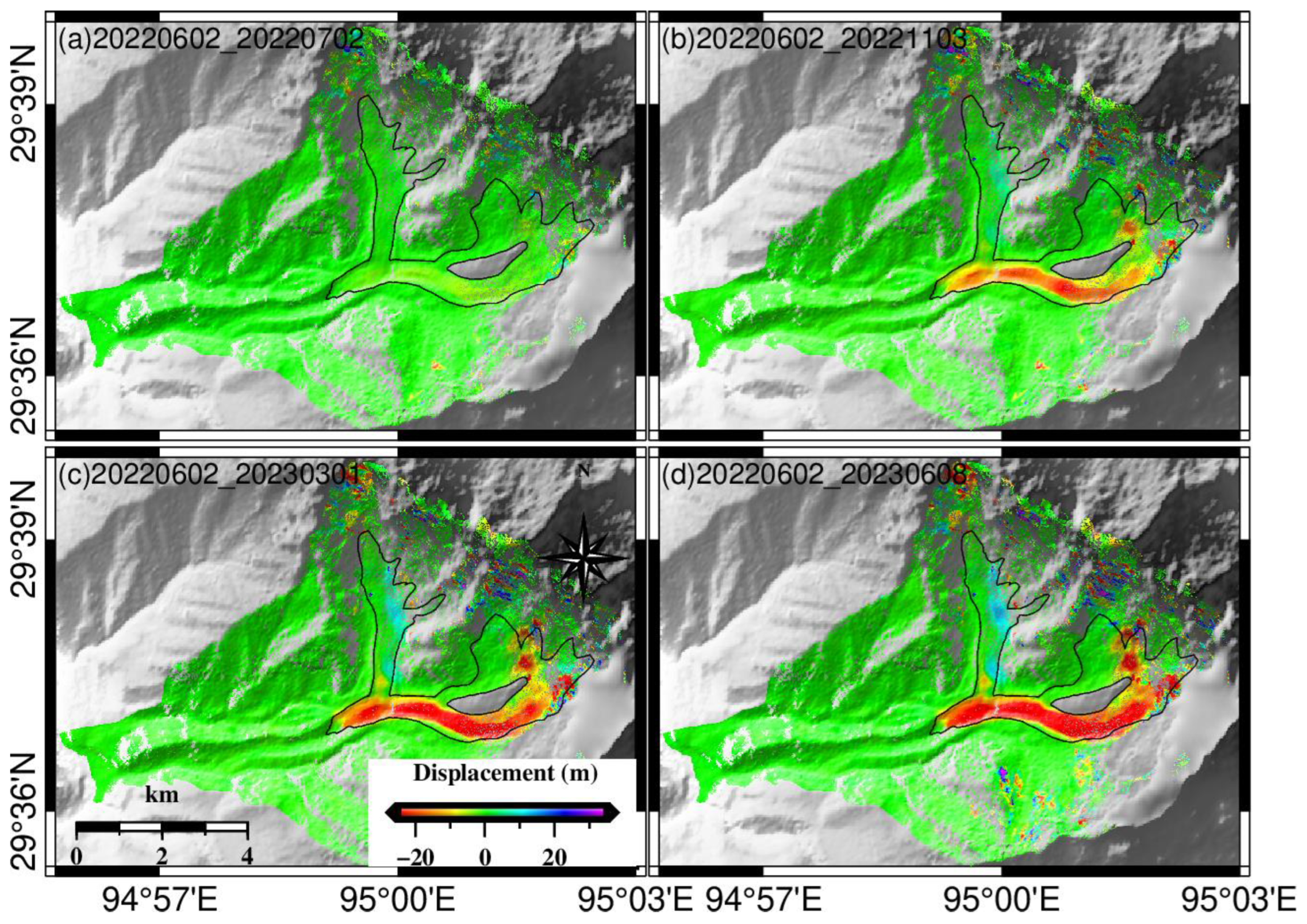
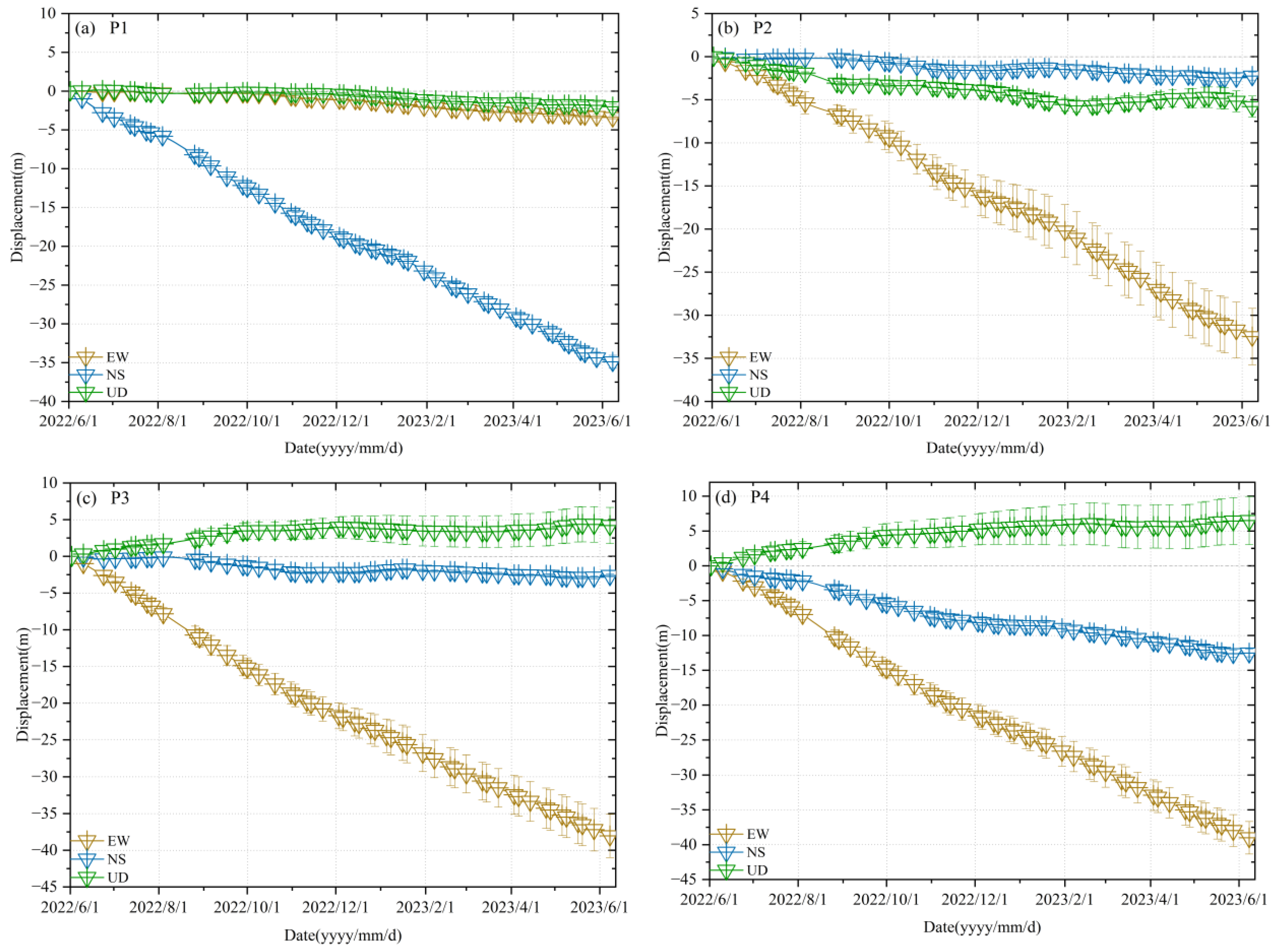
To further illustrate the temporal motion characteristics of the Zelongnong Glacier, the three-dimensional deformation time series from 2 June 2022 to 8 June 2023 were obtained using the PO-MSBAS method. The velocity time series in the east–west, north–south, and vertical directions are shown in Figure 6, Figure 7, and Figure 8, respectively. Six feature points along the glacier were selected (P1 to P4 shown in Figure 4). Figure 9 shows the time series displacement for each point, with the error bars representing the standard deviations in the horizontal and vertical directions, calculated within a 3 × 3 pixel surrounding the given pixel.
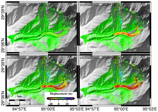
Figure 6.
Time series of EW glacier motion from 2 June 2022 to 8 June 2023.
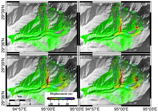
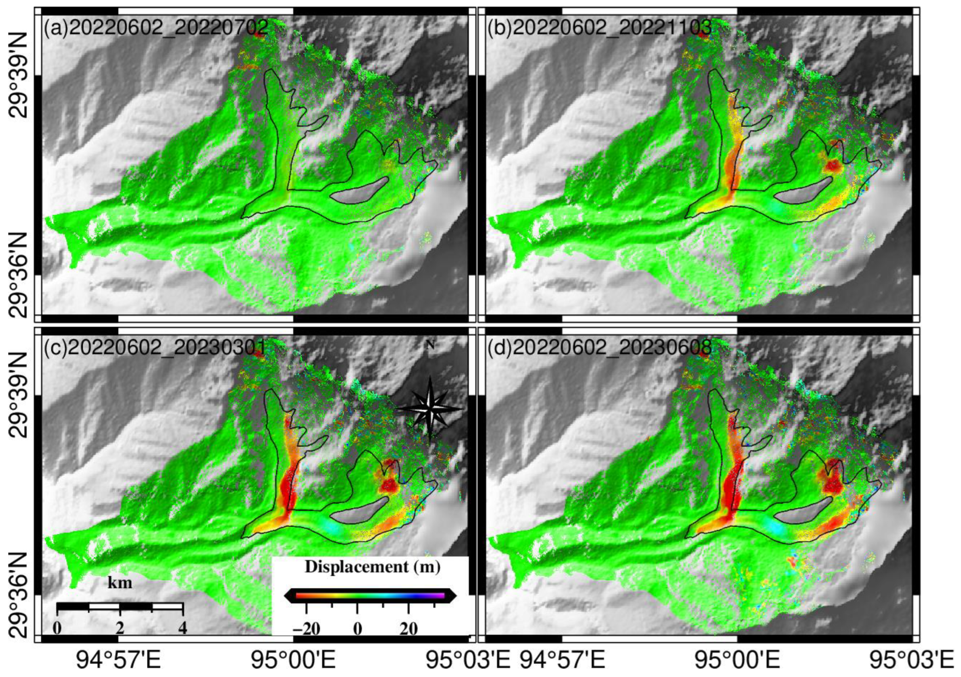
Figure 7.
Time series of NS glacier motion from 2 June 2022 to 8 June 2023.
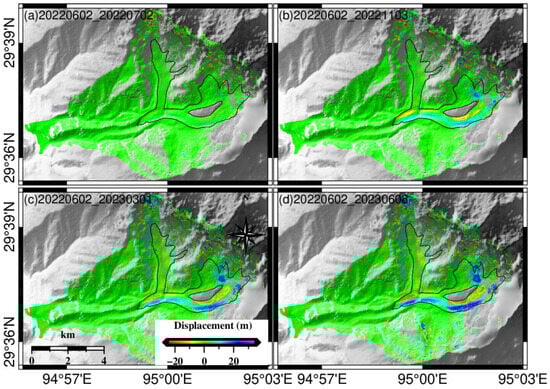
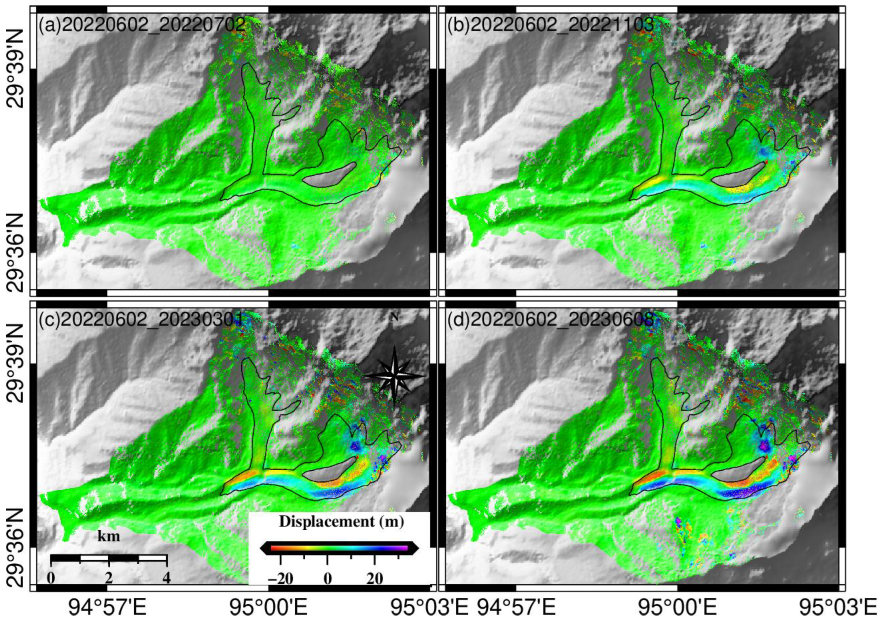
Figure 8.
Time series of UD glacier motion from 2 June 2022 to 8 June 2023.
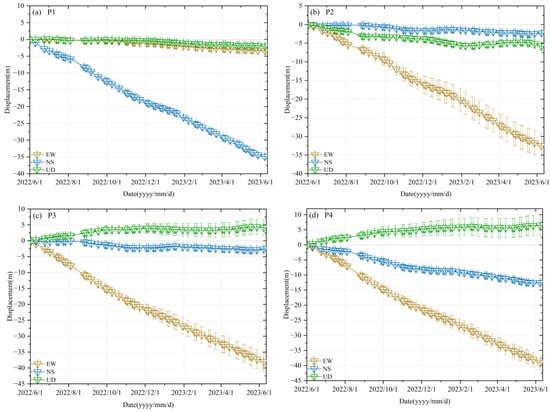
Figure 9.
Three-dimensional displacement time series for points P1–P4, where the positions are shown in Figure 4b.
The three-dimensional displacement time series of Zelongnong Glacier was analyzed as follows:
- (1)
- In Figure 6, Figure 7 and Figure 8, it is evident that the Zelongnong Glacier exhibited different motion characteristics in three directions. The glacier showed mainly east-to-west motion, with an obvious cumulative displacement towards the west in the southern tributary and the main stream. It then increased with time. In the north–south direction, the velocities were more pronounced in the central and right sections of the northern glacier tributary, while the velocity direction of the southern tributary changed from south to north at the bend, which is closely related to the terrain conditions. The northern sections of the southern tributaries and the main glacier experience ablation, while the southern sections of the southern tributaries and the main glacier show material accumulation, there is a clear stratification in the vertical movement between the northern and southern sections.
- (2)
- Figure 9 reveals that the displacement of P1, located in the central part of the northern tributary, changed slowly over time in the east–west and vertical directions but exhibited significant displacement changes in the north–south direction, with the maximum cumulative displacement over −34.88 ± 0.84 m. P2, located in the central southern region of the southern tributary, showed relatively small deformation in the north–south and vertical directions but substantial deformation in the east–west direction, with a maximum cumulative displacement of −32.47 ± 3.24 m, which is consistent with the three-dimensional displacement trend observed in the southern section of the tributary. P3, situated in the east–west glacier orientation, reached −38.04 ± 2.56 m east–west displacement due to the confluence of velocity from the two upper tributaries, which was greater than the one at P2. Lastly, P4, located in the middle of the mainstream, had a maximum cumulative displacement of around −39.00 ± 2.33 m in the east–west direction; the maximum cumulative displacement was −12.53 ± 0.52 m in the north–south direction, which was less than the one at P3 before two tributaries merged, as two tributaries had approximately perpendicular motion directions.
5. Discussion
5.1. The Comparison Between the Improved and Original Method
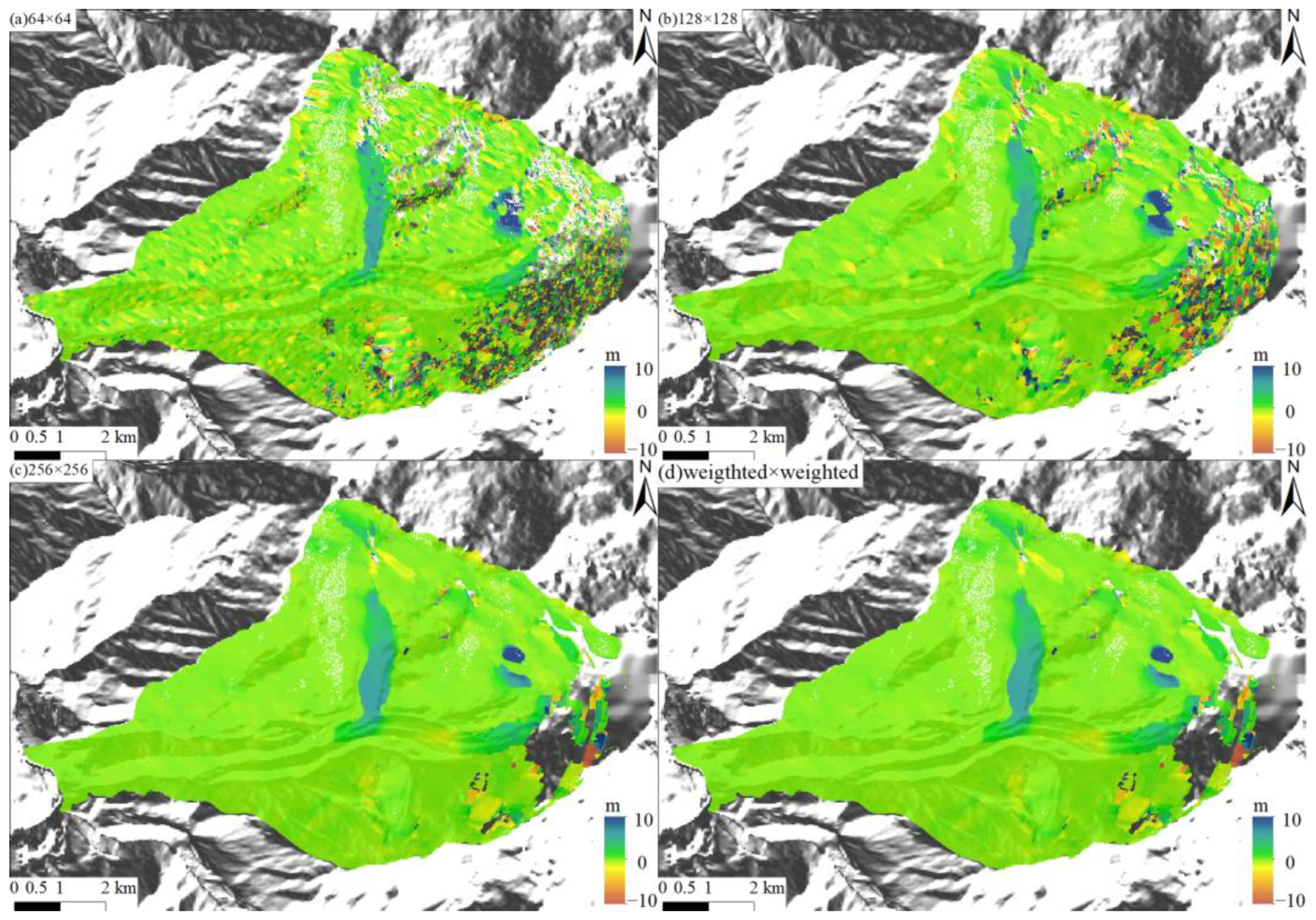
The size of the cross-correlation window has a considerable impact on the results when monitoring surface displacement using SAR offset tracking. In order to reduce the noise and integrate the advantages of different windows, this study proposes an offset tracking method based on the variable window-weighted cross-correlation strategy in Section 3.1. To validate the accuracy of this method, the offset pairs of ascending data from 25 March 2022 to 8 May 2022 were selected. Different sizes of a fixed single window (from 64 × 64 size to 256 × 256 size) and the method introduced in this study were utilized to obtain the azimuth offset results, as illustrated in Figure 10.
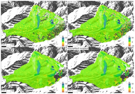
Figure 10.
The azimuth deformation was calculated using different methods: (a–c) the azimuth deformation calculated with different fixed window sizes; (d) the azimuth deformation calculated using the method proposed in this study.
The results demonstrate that smaller window sizes achieve a higher spatial resolution of the glacial deformation field in local areas, but they also increase noise. As the window size increases, the noise level in the deformation field gradually decreases, but this also leads to a loss of more deformation details. Consequently, it is challenging to obtain a reliable glacial deformation field with both high accuracy and spatial resolution using the commonly single fixed-window cross-correlation method. In contrast, Figure 10d demonstrates that the weighted method proposed in this study effectively balances information with noise levels in the glacial deformation field.
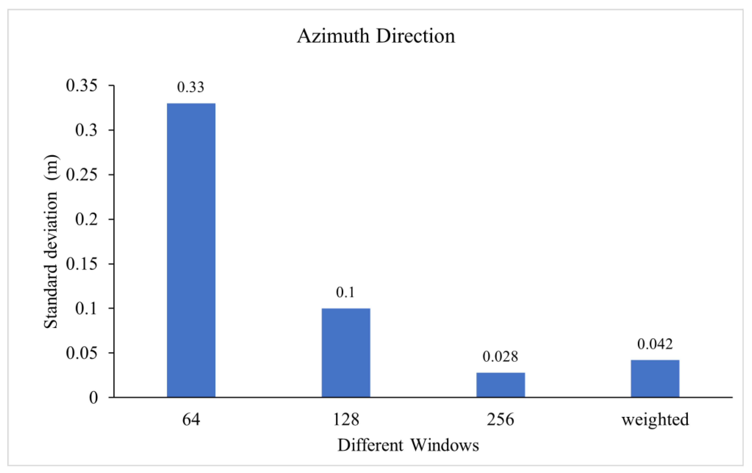
Additionally, we extracted the offset results from stable areas for accuracy assessment, selecting locations as shown in Figure 1b. The standard deviations of the azimuth results for different methods are presented in Figure 11. The standard deviations of the azimuth deformation exhibit exponential decay as the window size increases.
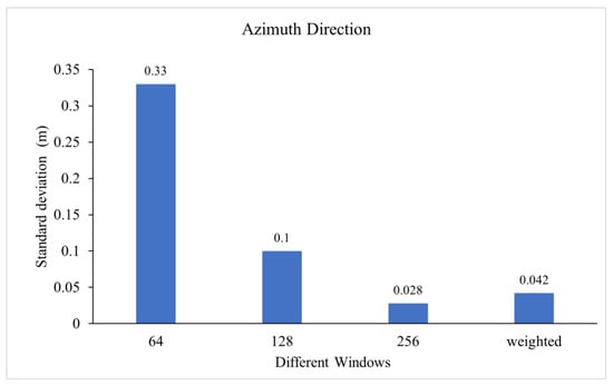
Figure 11.
The standard deviation of azimuth deformation with traditional and new methods.
The standard deviation of the deformation in the stable region of the proposed method is less than that obtained from the 128 × 128 fixed-window offset tracking and higher than that obtained from the 256 × 256 fixed-window offset tracking. In Figure 10, we can see that the deformation details are more pronounced than the results obtained from the 256 × 256 fixed-window offset tracking, while the noise level is lower than that from the 128 × 128 fixed-window offset tracking. In summary, this method is suitable for monitoring glaciers with significant gradient deformations.
5.2. Accuracy Assessment
The SAR image data used in this study are from TerraSAR/PAZ, which have high image resolution, and the registration accuracy can be ensured within 0.2 pixels, corresponding to 0.4 m in the azimuth direction and 0.27 m in the LOS direction. Based on the theory of zero motion in the non-glacier region, the observation error in the three-dimensional velocity was assessed with the standard deviation of ground deformation in the non-glacier regions as shown in Figure 1b. The results reveal the standard deviations of 0.25 m/year in the east–west direction, 0.16 m/year in the north–south direction, and 0.26 m/year in the vertical direction, which are significantly smaller than the average glacier velocity, indicating the higher reliability of the results [31].
5.3. Influencing Factors Analysis
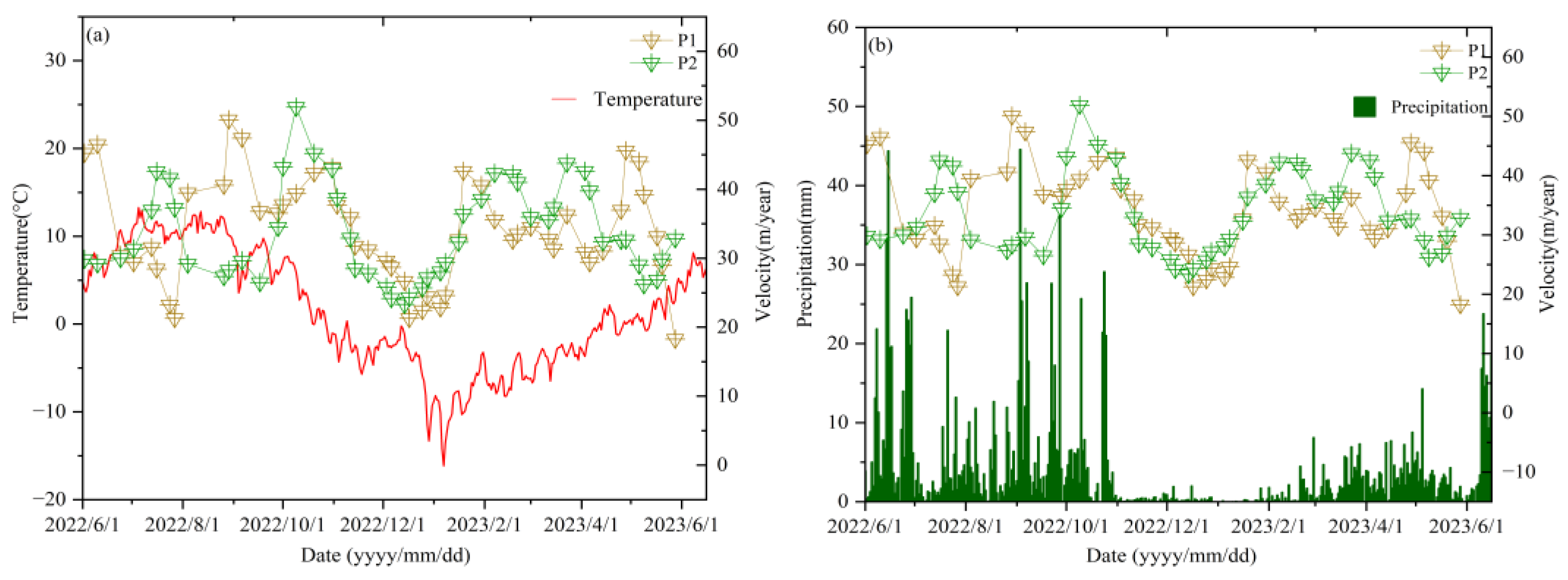
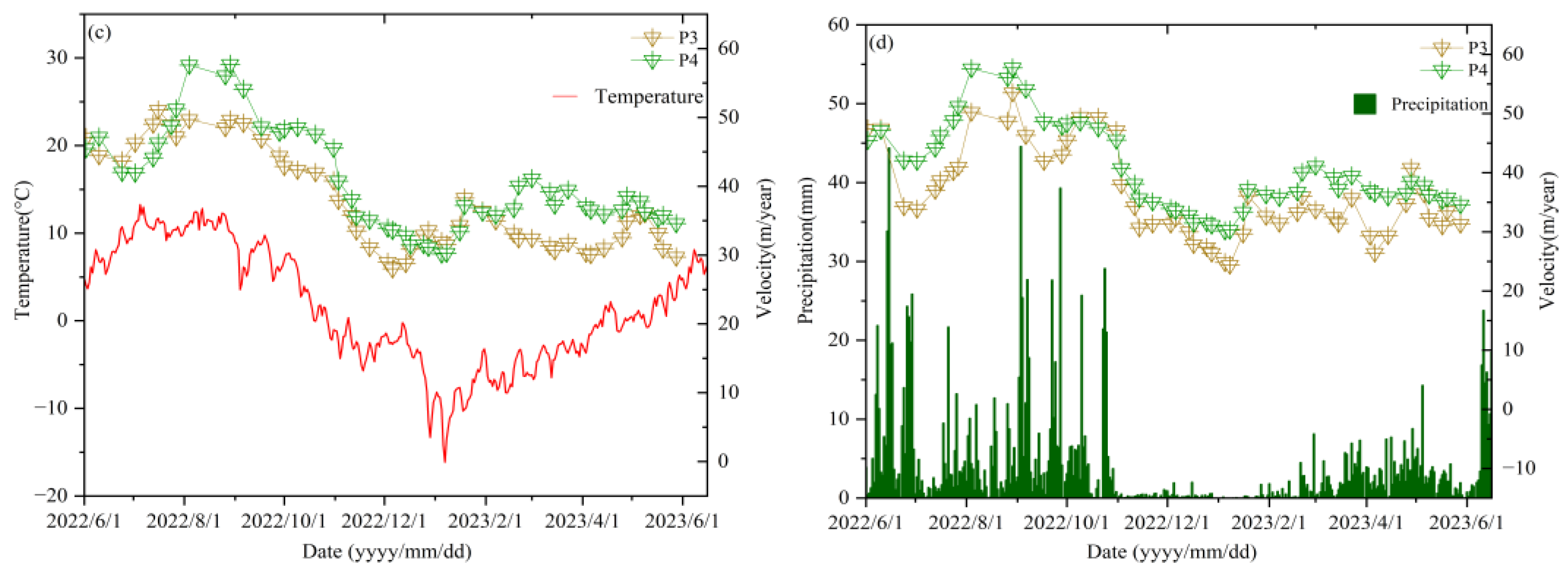
As a typical maritime glacier, Zelongnong Glacier is significantly influenced by summer monsoon precipitation and is more sensitive to climate changes compared to continental glaciers. To reveal the primary factors of glacier displacement variations, the correlation between temperature, precipitation, and glacier movement velocity at four feature points was analyzed as shown in Figure 12.
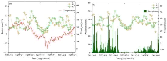

Figure 12.
The relationship between glacier velocity and temperature and precipitation. (a) Glacier velocity versus temperature at points P1–P2; (b) glacier velocity versus temperature at points P3–P4; (c) glacier velocity versus precipitation at points P1–P2; and (d) glacier velocity versus precipitation at points P3–P4.
The results were analyzed as follows:
- (1)
- Figure 12 reveals that temperatures remained below 0 °C from November 2022 to April 2023, and precipitation was below 5 mm from November 2022 to February of the following year. During this period, the velocity of the glacier at four points decreased significantly, which corresponds to the observed pattern in maritime glaciers, where velocity was higher in summer and lower in winter.
- (2)
- The correlation coefficients of P1 and P2 with temperature are 0.22 and 0.03, respectively, and with precipitation are 0.32 and 0.06. As P1 and P2 are both located at higher elevations on glacier tributaries, they follow the overall same trend as temperature and precipitation, but the changes are not uniform. The slope of the northern tributary where P1 is located varies significantly compared to the southern tributary and the mainstream, which may cause the response to temperature and precipitation changes to be influenced by the complex terrain effects. P2 is at the beginning of the turning point of the glacier tributary, controlled by the topographic conditions, where changes in glacier direction and stress distribution at the bend may reduce the influence of climatic factors on glacier velocity.
- (3)
- P3 and P4 present a more similar motion trend and higher correlations with temperature and precipitation compared to P1 and P2. The correlation coefficients with temperature are 0.79 and 0.78, and with precipitation are 0.44 and 0.53, respectively. They are both located in the central sections of the glacier’s tributary or mainstream, where the terrain is relatively flat, and the temperature and precipitation are more homogeneous and concentrated. Additionally, the central area is typically the main active region of glacier motion, making it more sensitive to temperature and precipitation changes.
To further investigate the common periodic characteristics and temporal relationships between glacier velocity and temperature and precipitation, we employed Wavelet Cross-Transform (WXT) for correlation analysis. The velocity time series for P3–P4, with better alignment with the variations in temperature and precipitation trends, were selected. Singular Spectrum Analysis (SSA) was first used to extract periodic components, followed by WXT to quantitatively study the lag effects between the two variables [29,32].
Figure 13 shows the cross-wavelet energy spectrum of the glacier velocity periodic components and temperature and precipitation series by performing the XWT, where arrows indicate the relative stage relationships: arrows pointing to the right represent stage changes in the same direction, while arrows pointing to the left indicate stage changes in the opposite direction. At the 95% confidence level, blue represents the lowest power within the cone of influence (COI), and yellow represents the highest power within the COI.
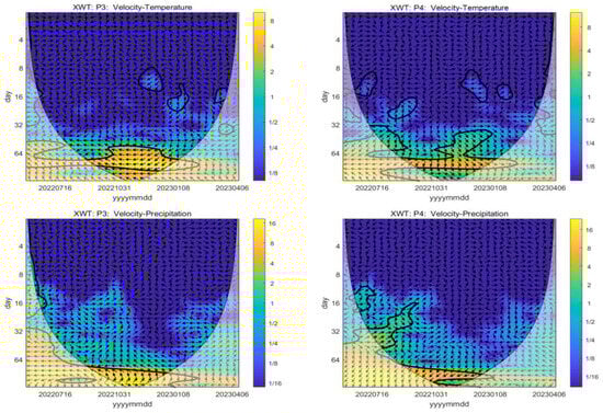
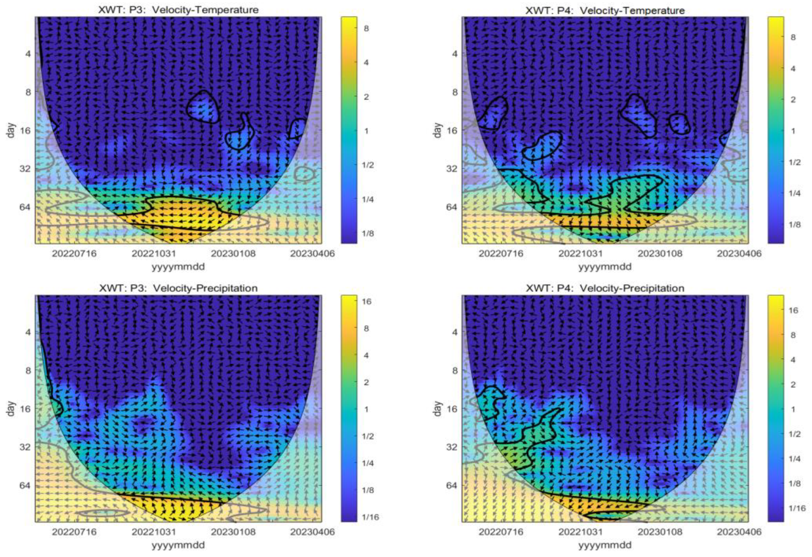
Figure 13.
Wavelet energy spectrum of glacier velocity crossed with temperature and precipitation.
As shown in Figure 13, the velocity of the two feature points exhibits higher wavelet power (yellow) with temperature and precipitation within the period of approximately one quarter (about 90 days), indicating a strong correlation between them. This periodic range likely corresponds to seasonal transitions, highlighting significant seasonal characteristics of the glacier.
Taking P4 as an example, the arrows in the cross-wavelet energy spectrum for temperature with a 90-day periodic band predominantly point downward, while those for precipitation mainly point southwest. This indicates that glacier velocity changes lag behind both temperature and precipitation.
In general, temperature and precipitation are the primary factors influencing glacier motion in this region, with temperature having a more significant impact. The characteristic points in the central part of the glacier are more sensitive to changes in temperature and precipitation compared to those in the upper sections. Glacier velocity has significant seasonal characteristics, and glacier velocity changes have a certain time lag compared with temperature and precipitation. However, given the complexity of glacier motion and the limited length of the time series, the cross-wavelet energy spectra also show some differences across different locations.
6. Conclusions
Zelongnong is one of the most developed areas for high-altitude, long-distance geological disasters. In this study, we use the PO-MSBAS method for high-resolution TerraSAR/PAZ images and propose a variable window-weighted cross-correlation strategy. This strategy effectively balances resolution and accuracy when using a single registration window size. It leverages the advantages of different window sizes, effectively reducing noise while retaining certain details in the offset results. Additionally, the standard deviation in the stable region is notably lower compared to traditional methods using smaller window sizes. The experimental results derived the three-dimensional motion field of Zelongnong Glacier from 2022 to 2023, and by characterizing the multidimensional spatial pattern and temporal evolution of the glacier, the results demonstrated that the southern glacier tributary had a higher velocity than the northern one. In the northern tributary, the maximum horizontal velocity reached 45.07 m/year, while the vertical velocity was −7.45 m/year, and the southern tributary reached 50.15 m/year in the horizontal direction and 50.66 m/year in the vertical direction. The southern tributary undergoes two bends before merging with the mainstream, displaying a more complex motion pattern.
The correlations among glacier velocity and temperature and precipitation revealed that the glacier moved faster in summer and slower in winter, which is consistent with the characteristics of maritime glaciers. Furthermore, the central regions of the glacier were more sensitive to the changes in temperature and precipitation. The glacier velocity was influenced by the combined effects of temperature and precipitation, with temperature having a more pronounced impact than precipitation.
Finally, glacier motion is a long-term evolutionary process. The short-term glacier motion analysis limits the ability to infer long-term glacier movement patterns. So it is essential to obtain much more remote sensing data with a longer period for long-term deformation monitoring to assess the risk of glacier-induced geohazard chains in the future.
Author Contributions
Conceptualization, X.Z. and C.Z.; data curation, X.Z. and X.L.; formal analysis, X.Z.; funding acquisition, C.Z. and B.L.; investigation, X.Z., C.Z. and W.W.; methodology, X.Z., X.L. and C.Z.; project administration, C.Z. and W.W.; resources, C.Z. and B.L.; software, X.Z. and X.L.; supervision, B.L. and C.Z.; validation, X.Z. and C.Z.; visualization, X.Z., B.L. and W.W.; writing—original draft, X.Z.; writing—review and editing, C.Z. All authors have read and agreed to the published version of the manuscript.
Funding
This work was funded by the National Key R&D Program of China (No. 2022YFC3004302) and the National Natural Science Foundation of China (Grant No. 42474029).
Data Availability Statement
The data are available from the corresponding author upon reasonable request.
Acknowledgments
We thank the German Aerospace Center (DLR) for providing the TerraSAR-X data under grant No. MTH3809 and the Spanish National Institute of Aerospace Technology for providing the PAZ images under grant No. AO-003-028. The precipitation and temperature data were downloaded from the websites https://gpm.nasa.gov/ (accessed on 13 January 2024) and https://cds.climate.copernicus.eu/ (accessed on 9 January 2024). This work was also supported by the Chang’an University High Performance Computing Platform.
Conflicts of Interest
The authors declare no conflicts of interest.
References
- Hugonnet, R.; McNabb, R.; Berthier, E.; Menounos, B.; Nuth, C.; Girod, L.; Farinotti, D.; Huss, M.; Dussaillant, I.; Brun, F.; et al. Accelerated Global Glacier Mass Loss in the Early Twenty-First Century. Nature 2021, 592, 726–731. [Google Scholar] [CrossRef] [PubMed]
- An, B.; Wang, W.; Yang, W.; Wu, G.; Guo, Y.; Zhu, H.; Gao, Y.; Bai, L.; Zhang, F.; Zeng, C.; et al. Process, Mechanisms, and Early Warning of Glacier Collapse-Induced River Blocking Disasters in the Yarlung Tsangpo Grand Canyon, Southeastern Tibetan Plateau. Sci. Total Environ. 2022, 816, 151652. [Google Scholar] [CrossRef] [PubMed]
- Li, G.; Zhao, C.; Wang, B.; Peng, M.; Bai, L. Evolution of Spatiotemporal Ground Deformation over 30 Years in Xi’an, China, with Multi-Sensor SAR Interferometry. J. Hydrol. 2023, 616, 128764. [Google Scholar] [CrossRef]
- Li, J.; Li, Z.; Ding, X.; Wang, Q.; Zhu, J.; Wang, C. Investigating Mountain Glacier Motion with the Method of SAR Intensity-Tracking: Removal of Topographic Effects and Analysis of the Dynamic Patterns. Earth-Sci. Rev. 2014, 138, 179–195. [Google Scholar] [CrossRef]
- Li, W.; Chen, J.; Lu, H.; Yu, C.; Shan, Y.; Li, Z.; Dong, X.; Xu, Q. Analysis of Seismic Impact on Hailuogou Glacier after the 2022 Luding Ms 6.8 Earthquake, China, Using SAR Offset Tracking Technology. Remote Sens. 2023, 15, 1468. [Google Scholar] [CrossRef]
- Cai, J.; Zhang, L.; Dong, J.; Wang, C.; Liao, M. Polarimetric SAR Pixel Offset Tracking for Large-Gradient Landslide Displacement Mapping. Int. J. Appl. Earth Obs. Geoinf. 2022, 112, 102867. [Google Scholar] [CrossRef]
- Du, S.; Mallorqui, J.J.; Zhao, F. Patch-Like Reduction (PLR): A SAR Offset Tracking Amplitude Filter for Deformation Monitoring. Int. J. Appl. Earth Obs. Geoinf. 2022, 113, 102976. [Google Scholar] [CrossRef]
- Li, S.; Leinss, S.; Hajnsek, I. Cross-Correlation Stacking for Robust Offset Tracking Using SAR Image Time-Series. IEEE J. Sel. Top. Appl. Earth Obs. Remote Sens. 2021, 14, 4765–4778. [Google Scholar] [CrossRef]
- Yang, Z.; Li, Z.; Zhu, J.; Preusse, A.; Hu, J.; Feng, G.; Yi, H.; Papst, M. An Alternative Method for Estimating 3-D Large Displacements of Mining Areas from a Single SAR Amplitude Pair Using Offset Tracking. IEEE Trans. Geosci. Remote Sens. 2018, 56, 3645–3656. [Google Scholar] [CrossRef]
- Guo, L.; Li, J.; Li, Z.; Wu, L.; Li, X.; Hu, J.; Li, H.; Li, H.; Miao, Z.; Li, Z. The Surge of the Hispar Glacier, Central Karakoram: SAR 3-D Flow Velocity Time Series and Thickness Changes. J. Geophys. Res. Solid Earth 2020, 125, e2019JB018945. [Google Scholar] [CrossRef]
- Shi, Y.; Liu, G.; Wang, X.; Liu, Q.; Shum, C.K.; Bao, J.; Mao, W. Investigating the Intra-Annual Dynamics of Kunlun Glacier in the West Kunlun Mountains, China, From Ascending and Descending Sentinel-1 SAR Observations. IEEE J. Sel. Top. Appl. Earth Obs. Remote Sens. 2022, 15, 1272–1282. [Google Scholar] [CrossRef]
- Yang, L.; Zhao, C.; Lu, Z.; Yang, C.; Zhang, Q. Three-Dimensional Time Series Movement of the Cuolangma Glaciers, Southern Tibet with Sentinel-1 Imagery. Remote Sens. 2020, 12, 3466. [Google Scholar] [CrossRef]
- Guo, R.; Jiang, L.; Xu, Z.; Li, C.; Huang, R.; Zhou, Z.; Li, T.; Liu, Y.; Wang, H.; Fan, X. Seismic and Hydrological Triggers for a Complex Cascading Geohazard of the Tianmo Gully in the Southeastern Tibetan Plateau. Eng. Geol. 2023, 324, 107269. [Google Scholar] [CrossRef]
- Wang, W.; Yang, J.; Wang, Y. Dynamic Processes of 2018 Sedongpu Landslide in Namcha Barwa–Gyala Peri Massif Revealed by Broadband Seismic Records. Landslides 2020, 17, 409–418. [Google Scholar] [CrossRef]
- Jiang, R.; Zhang, L.; Peng, D.; He, X.; He, J. The Landslide Hazard Chain in the Tapovan of the Himalayas on 7 February 2021. Geophys. Res. Lett. 2021, 48, e2021GL093723. [Google Scholar] [CrossRef]
- Li, Z.; Sun, J.; Gao, M.; Fu, G.; An, Z.; Zhao, Y.; Fang, L.; Guo, X. Evaluation of Horizontal Ground Motion Waveforms at Sedongpu Glacier during the 2017 M6.9 Mainling Earthquake Based on the Equivalent Green’s Function. Eng. Geol. 2022, 306, 106743. [Google Scholar] [CrossRef]
- Zhang, J.; Shen, X. Debris-Flow of Zelongnong Ravine in Tibet. J. Mt. Sci. 2011, 8, 535–543. [Google Scholar] [CrossRef]
- Liang, Q.; Wang, N. Mountain Glacier Flow Velocity Retrieval from Ascending and Descending Sentinel-1 Data Using the Offset Tracking and MSBAS Technique: A Case Study of the Siachen Glacier in Karakoram from 2017 to 2021. Remote Sens. 2023, 15, 2594. [Google Scholar] [CrossRef]
- Raucoules, D.; De Michele, M.; Malet, J.-P.; Ulrich, P. Time-Variable 3D Ground Displacements from High-Resolution Synthetic Aperture Radar (SAR). Application to La Valette Landslide (South French Alps). Remote Sens. Environ. 2013, 139, 198–204. [Google Scholar] [CrossRef]
- Chae, S.-H.; Lee, W.-J.; Baek, W.-K.; Jung, H.-S. An Improvement of the Performance of SAR Offset Tracking Approach to Measure Optimal Surface Displacements. IEEE Access 2019, 7, 131627–131637. [Google Scholar] [CrossRef]
- Liu, X.; Zhao, C.; Zhang, Q.; Lu, Z.; Li, Z. Deformation of the Baige Landslide, Tibet, China, Revealed Through the Integration of Cross-Platform ALOS/PALSAR-1 and ALOS/PALSAR-2 SAR Observations. Geophys. Res. Lett. 2020, 47, e2019GL086142. [Google Scholar] [CrossRef]
- Luckman, A.; Quincey, D.; Bevan, S. The Potential of Satellite Radar Interferometry and Feature Tracking for Monitoring Flow Rates of Himalayan Glaciers. Remote Sens. Environ. 2007, 111, 172–181. [Google Scholar] [CrossRef]
- Yan, S.; Liu, G.; Wang, Y.; Perski, Z.; Ruan, Z. Glacier Surface Motion Pattern in the Eastern Part of West Kunlun Shan Estimation Using Pixel-Tracking with PALSAR Imagery. Env. Earth Sci. 2015, 74, 1871–1881. [Google Scholar] [CrossRef]
- Yin, Y.; Liu, X.; Zhao, C.; Tomás, R.; Zhang, Q.; Lu, Z.; Li, B. Multi-Dimensional and Long-Term Time Series Monitoring and Early Warning of Landslide Hazard with Improved Cross-Platform SAR Offset Tracking Method. Sci. China Technol. Sci. 2022, 65, 1891–1912. [Google Scholar] [CrossRef]
- Samsonov, S.; d’Oreye, N. Multidimensional Time-Series Analysis of Ground Deformation from Multiple InSAR Data Sets Applied to Virunga Volcanic Province. Geophys. J. Int. 2012, 191, 1095–1108. [Google Scholar] [CrossRef]
- Samsonov, S.V.; d’Oreye, N.; González, P.J.; Tiampo, K.F.; Ertolahti, L.; Clague, J.J. Rapidly Accelerating Subsidence in the Greater Vancouver Region from Two Decades of ERS-ENVISAT-RADARSAT-2 DInSAR Measurements. Remote Sens. Environ. 2014, 143, 180–191. [Google Scholar] [CrossRef]
- Samsonov, S.; Dille, A.; Dewitte, O.; Kervyn, F.; d’Oreye, N. Satellite Interferometry for Mapping Surface Deformation Time Series in One, Two and Three Dimensions: A New Method Illustrated on a Slow-Moving Landslide. Eng. Geol. 2020, 266, 105471. [Google Scholar] [CrossRef]
- Samsonov, S.; Tiampo, K.; Cassotto, R. Measuring the State and Temporal Evolution of Glaciers in Alaska and Yukon Using Synthetic-Aperture-Radar-Derived (SAR-Derived) 3D Time Series of Glacier Surface Flow. Cryosphere 2021, 15, 4221–4239. [Google Scholar] [CrossRef]
- Torrence, C.; Compo, G.P. A Practical Guide to Wavelet Analysis. Bull. Amer. Meteor. Soc. 1998, 79, 61–78. [Google Scholar] [CrossRef]
- Nye, J.F. The Motion of Ice Sheets and Glaciers. J. Glaciol. 1959, 3, 493–507. [Google Scholar] [CrossRef]
- Li, J.; Li, Z.; Wu, L.; Xu, B.; Hu, J.; Zhou, Y.; Miao, Z. Deriving a Time Series of 3D Glacier Motion to Investigate Interactions of a Large Mountain Glacial System with Its Glacial Lake: Use of Synthetic Aperture Radar Pixel Offset-Small Baseline Subset Technique. J. Hydrol. 2018, 559, 596–608. [Google Scholar] [CrossRef]
- Hassani, H. Singular Spectrum Analysis: Methodology and Comparison. J. Data Sci. 2021, 5, 239–257. [Google Scholar] [CrossRef]


Disclaimer/Publisher’s Note: The statements, opinions and data contained in all publications are solely those of the individual author(s) and contributor(s) and not of MDPI and/or the editor(s). MDPI and/or the editor(s) disclaim responsibility for any injury to people or property resulting from any ideas, methods, instructions or products referred to in the content. |
© 2024 by the authors. Licensee MDPI, Basel, Switzerland. This article is an open access article distributed under the terms and conditions of the Creative Commons Attribution (CC BY) license (https://creativecommons.org/licenses/by/4.0/).