Article

Estimation of Urban Tree Chlorophyll Content and Leaf Area Index Using Sentinel-2 Images and 3D Radiative Transfer Model Inversion

1
UMR 6554 CNRS, LETG, University of Rennes, Place du Recteur Henri Le Moal, 35000 Rennes, France
2
DOTA, ONERA, Université de Toulouse, 31055 Toulouse, France
*
Author to whom correspondence should be addressed.
Remote Sens. 2024, 16(20), 3867; https://doi.org/10.3390/rs16203867
Submission received: 6 September 2024 / Revised: 12 October 2024 / Accepted: 16 October 2024 / Published: 18 October 2024
(This article belongs to the Special Issue Urban Sensing Methods and Technologies II)

Abstract

:
Urban trees play an important role in mitigating effects of climate change and provide essential ecosystem services. However, the urban environment can stress trees, requiring the use of effective monitoring methods to assess their health and functionality. The objective of this study, which focused on four deciduous tree species in Rennes, France, was to evaluate the ability of hybrid inversion models to estimate leaf chlorophyll content (LCC), leaf area index (LAI), and canopy chlorophyll content (CCC) of urban trees using eight Sentinel-2 (S2) images acquired in 2021. Simulations were performed using the 3D radiative transfer model DART, and the hybrid inversion models were developed using machine-learning regression algorithms (random forest (RF) and gaussian process regression). Model performance was assessed using in situ measurements, and relations between satellite data and in situ measurements were investigated using spatial allocation (SA) methods at the pixel and tree scales. The influence of including environment features (EFs) as model inputs was also assessed. The results indicated that random forest models that included EFs and used the pixel-scale SA method were the most accurate with R2 values of 0.33, 0.29, and 0.46 for LCC, LAI, and CCC, respectively, with notable variability among species.

1. Introduction

In the realm of climate-change mitigation, urban trees play a central role in the strategies of land-use planning because they provide a variety of essential ecosystem services [1,2], such as temperature regulation by providing shade and evapotranspiration [3], carbon storage [4], and biodiversity preservation [5]. As a result, the presence of vegetation in urban areas is crucial for human health and the overall quality of life [6]. However, the urban environment contains many stress factors that can slow tree development [7]. Urban trees can experience mechanical and chemical disturbances due to planting conditions (proximity to buildings, edaphic conditions), and atmospheric conditions such as temperature and air quality, and light pollution at night. While urban trees contribute significantly to urban well-being, they must contend with a limiting environment that can damage their health. Several studies demonstrate notable impacts of these stress factors: urban trees have a shorter lifespan than rural trees [8], isolated and street trees experience more stress than those in parks [9], and young trees have a higher mortality rate in urban areas [10].
In this context, effectively monitoring the functional and mechanical condition of urban trees at a large scale is challenging. Traditional field inventories of urban trees are usually limited to a few trees and are performed annually or even every 10 years because they require large amounts of human resources and time. Conversely, satellite remote sensing can collect information on urban vegetation across entire cities with both high spatial and temporal resolutions. Over the past decade, the use of satellite remote sensing in urban areas for vegetation-related purposes has grown steadily [11,12]. Most studies have focused on mapping large urban green spaces and classifying the species in them. Relatively fewer studies have concentrated on smaller vegetation patches such as isolated or aligned street trees, despite a large amount of cumulative coverage of such patches. Furthermore, few studies have investigated the functional status of urban trees to assess health or estimate biomass, instead focussing mainly on large green infrastructures. Vegetation status can be characterized using proxies, which can be estimated using models based on satellite images. The most commonly used vegetation traits are (i) leaf chlorophyll content (LCC), often expressed in µg of chlorophyll a and b per cm2 of leaf; (ii) leaf area index (LAI), which corresponds to the sum of leaf areas of the tree crown relative to the tree crown projection at ground area expressed in m2/m2; and (iii) canopy chlorophyll content (CCC), expressed in µg/cm2, which is the product of LCC and LAI. LCC is closely linked to photosynthetic activity [13,14], biomass production [15,16], and levels of air and soil pollution [17]. Because chlorophyll pigments are sensitive to changes in external conditions, LCC is a good indicator of environmental stress and changes in temperature and humidity [18]. At the canopy scale, LAI can be used to identify tree phenological stages [19] and their photosynthetic potential [20]. CCC provides a more holistic and accurate representation of chlorophyll content at the canopy scale than leaf-scale estimates. These three vegetation traits can be estimated using satellite hyperspectral data due to the latter’s wide spectral range (0.4–2.5 µm) [21]. However, current satellite hyperspectral images, such as EnMAP and PRISMA images, have spatial and temporal resolutions that are too coarse (30 m and 27–29 days at nadir) for the study of urban trees. While high or very high spatial resolution (0.5–5 m) multispectral satellite imagery such as WorldView, RapidEye, Pleiades, QuickBird, and PlanetScope are increasingly used to study vegetation in urban environments, these data are not freely accessible conversely to Sentinel-2 (S2) imagery. S2 stands out for its high spatial resolution (10 m for visible and near infrared and 20 m for red edge (RE) (0.67–0.76 µm)/short-wave infrared), relatively large number of spectral bands (10 bands at 10–20 m resolution), and temporal resolution suited to monitoring intra-annual vegetation dynamics [22].
The methods used most often to estimate vegetation traits using S2 data can be classified into two main types [23]: empirical or physical. Empirical methods are based on regression models that derive empirical relationships between spectral bands or vegetation indices and the variable of interest (e.g., LCC, LAI). Statistical models are widely used due to their accessibility and ease of application. However, models developed for specific locations or sensor configurations face limitations when applied in other contexts, such as different vegetation types, sensor configurations, or data acquisition times. These limitations arise from the need for large and heterogeneous in situ datasets for model training and validation.
Physical methods are based on the use of radiative transfer models (RTM) to generate synthetic spectral datasets or Look-Up Tables (LUT) mimicking the simulation of remote sensing images. RTM models simulate the physical processes of electromagnetic radiation in a medium. In remote sensing, these models are used to generate synthetic images based on the optical and geometric properties of the scene and according to the characteristics of a given sensor. They can be divided into two subcategories: LUT-based models and hybrid models. LUT-based methods rely on the minimization of a cost function computed between the simulated (from LUT) and measured spectra for each pixel of the remote sensing image. Post-processing can include the use of adapted spectral intervals or the use of vegetation indices. The best fit should provide the most appropriate estimated variable value found in the LUT. The hybrid models rely on machine learning algorithms (MLRA) to train a model on the LUT before being applied on the remote sensing images to derive inversion maps of vegetation traits. In average, they are increasingly used, since they exploit the potential of physically based methods combined with the flexibility and computational efficiency of MLRA [23]. Moreover, predicting variables using lookup-table-based approaches may be less accurate, as different combinations of the input parameters can produce the same simulated spectra [24], especially in urban environments that contain many light interactions and a variety of objects and materials.
Hybrid inversion methods are well-suited for complex systems or scenarios in which traditional inversion methods may be insufficient. They can represent non-linear relationships, multi-scale processes, and interactions among components more effectively, making them suitable for studying intricate environmental phenomena such as those in urban contexts. By using hybrid inversion models with S2 data, many studies have succeeded in estimating vegetation traits, such as LCC in open-canopy conifer forests [25], LCC and LAI in deciduous broadleaf forests [26], and LCC, LAI, and CCC in mixed mountain forests [27]. In the same way, hybrid methods accurately estimated LAI and LCC in cropland [28,29].
These studies used the PROSPECT model [30,31] to simulate leaf reflectance and either SAIL [32] or INFORM [33] to simulate canopy reflectance. SAIL simulates the canopy as a horizontal turbid medium, whose properties depend on a simple representation of the canopy through the LAI and the leaf angle distribution. PROSAIL, which corresponds to the combined PROSPECT and SAIL models [34], has been extensively used for LAI and LCC retrieval of crops [35,36] and forests [37] due to its relative simplicity and accuracy. However, PROSAIL cannot accurately simulate the interactions occurring in complex canopies and environments in three dimensions such as urban canopies. INFORM can simulate more complex canopy structures [26] but cannot represent 3D scenes analogous to an urban environment. Choosing an RTM adapted to the context and able to model the complexity of interactions among the multiple scene components is essential for estimating vegetation traits in urban environments. The discrete anisotropic radiative transfer model (DART) [38,39] has many advantages for modelling three-dimensional (3D) urban scenes [40]. For example, DART has been used with S2 to retrieve the albedo of urban canopies [41] and the LCC and LAI of the sparse canopy of olive trees [42]. The latter study has similarities with this study, since the canopy of sparse olive plants is also heterogenous with a high variability in the optical properties of the ground, leading to a high proportion of S2 mixed pixels.
To our knowledge, no study has used S2 images to estimate vegetation traits of trees in urban areas. DART can simulate an urban scene, including the diversity of materials, the layout of buildings, the structure of the canopy, and its optical properties. These elements are essential for modelling a pseudo-realistic scene that reflects the heterogeneity of mixed pixels, which are common in urban remote sensing. In this study, we used a global approach to model urban trees that covers many urban configurations based on the definition of local climate zones (LCZ). The LCZ classification system provides a characterization of the physical nature of urban morphology, with LCZs defined as areas of uniform surface cover, structure, materials, and human activity that span hundreds of meters to several kilometers [43]. Originally, this classification system was dedicated to the study of urban climate and heat islands, but it is increasingly used as a reference framework for studying urban vegetation [44].
Among the MLRAs used with hybrid inversion approaches, random forest regression (RFR) [45] and Gaussian process regression (GPR) [46] are widely used. A study that compared MLRAs used with hybrid inversion showed that RFR and GPR slightly outperformed artificial neural network and support vector machines [27]. In the hybrid inversion studies cited, MLRAs were always trained with spectral features or derived features (vegetation indices). From images simulated by DART, pixel-level features can be estimated, such as the proportion of shadow, underlying vegetation, or canopy cover. These features can be used as training features and can improve model performance, as they interact with spectral features.
Finally, an important point when estimating vegetation traits using remote sensing is the approach used to combine field and satellite observations. Because field datasets are essential for validating predictions, in situ measurement protocols must be adapted to the spatial resolution of the images to ensure spatial consistency between the two data sources. For heterogeneous canopies that cover a large area, the most common method is to perform in situ measurements at the plot scale and extract the pixel values that correspond spatially to the plot. In this study, we used two spatial allocation (SA) methods, one at tree-scale and the other at pixel-scale. The tree-scale method simply assigns the vegetation traits of the dominant tree (i.e., the one with the largest crown area in the pixel) to the pixel. The pixel-scale method is more comprehensive and considered the percentage of tree(s) at the pixel scale by weighting the vegetation traits of the tree(s) by their crown area in the pixel. The two methods were evaluated and used to build the LUTs (i.e., to match the DART input parameters (LAI and LCC) and simulated pixel values) and for the validation step (i.e., to match in situ measurements and real S2 pixels). The aim of the study was to evaluate the performance of hybrid inversion models for estimating LCC, LAI, and CCC of urban trees from S2 images. Specifically, three components were investigated to determine the best strategy for estimating vegetation traits: (i) the contribution of environmental features (EFs) to training models, (ii) the spatial allocation (SA) method used to match vegetation traits and pixel values, and (iii) the MLRA used (RFR or GPR) to estimate vegetation traits.

2. Materials and Methods

2.1. Study Sites

The study sites were located in Rennes, in northwestern France (48°10′N, 1°68′W) (Figure 1a,b). Rennes is a medium-sized city of 222,485 inhabitants, with a population density of 4414 people/km2 (INSEE, 2020) [47]. Rennes is located in an oceanic climate zone, with a projected increase in mean annual temperature from 12.4 °C to 12.9 °C and 13.2 °C for representative concentration pathway scenarios 4.5 and 8.5, respectively, from 1991–2020 to 2031–2060 (Haut Conseil pour le Climat en Bretagne 2023) [48]. Rennes managed 130,000 trees in 2023 in public areas, including trees in parks, ornamental trees, and street trees. This study focused on four of the five most common deciduous genera in Rennes—oak (Quercus), maple (Acer), plane (Platanus), and ash (Fraxinus)—as deciduous trees are the dominant trees in Rennes. We chose to focus on trees with a crown diameter of at least 10 m, to ensure that the proportion of tree canopy in the Sentinel-2 pixel was sufficiently high. Therefore, we excluded linden trees (Tilia), the fifth most common deciduous genus, which is often pruned into a rectangular shape, which restricts the extent of the crown as seen from the zenith. We selected the most common species for each genus: Platanus acerifolia (PL), Quercus rubra (QR), Acer platanoides (AC), and Fraxinus excelsior (FR). A total of 117 trees were monitored in four monospecific alignments composed of 29 PL, 29 AC, 30 QR, and 29 FR (Figure 1c–f).

2.2. Methodological Framework

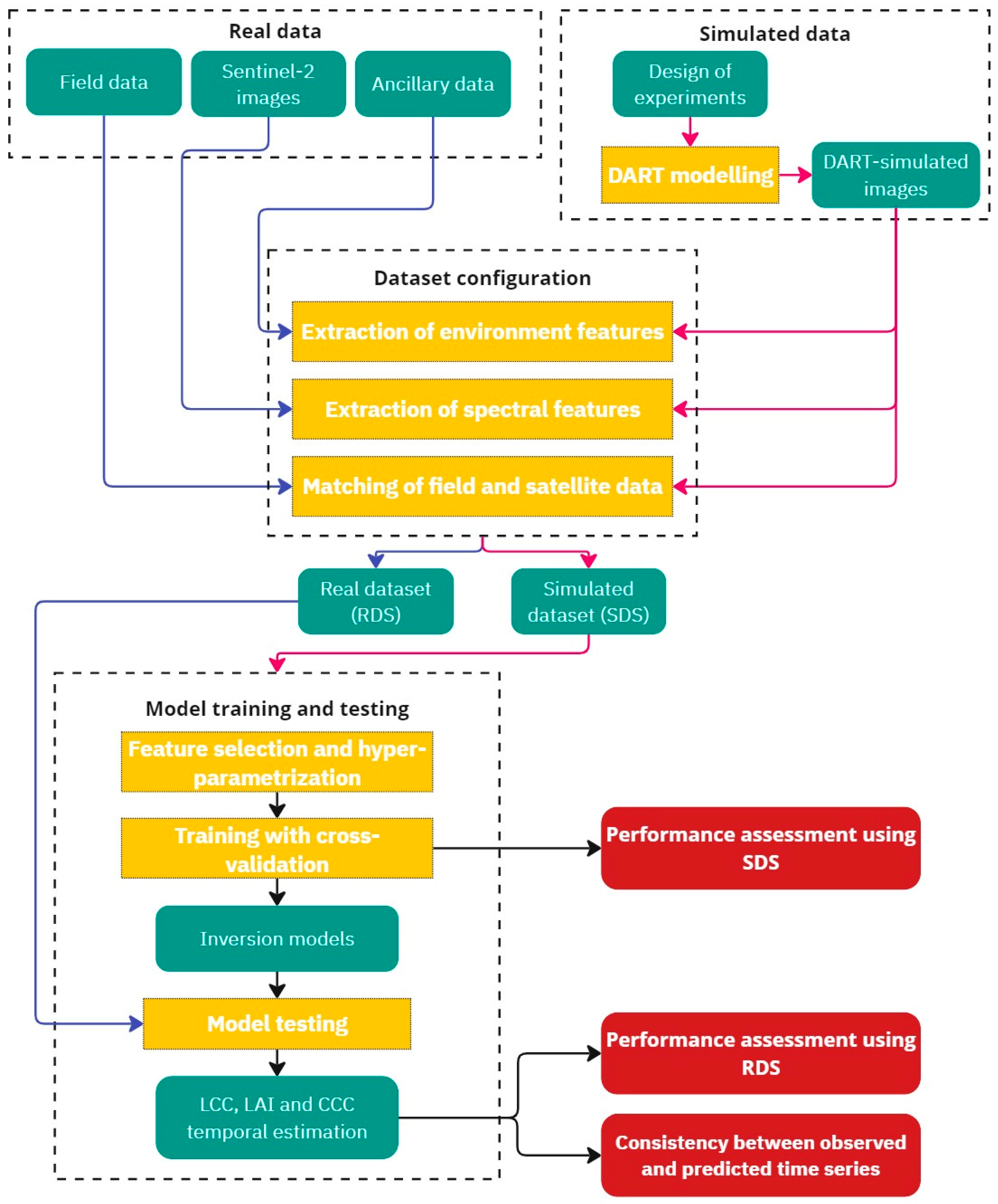
Tree vegetation traits were estimated from S2 images in four steps (Figure 2): (1) collection of real data to create a validation dataset that included field data, S2 images, and ancillary data; (2) simulation of S2 images based on a design of experiment and DART modelling/simulations; (3) configuration of the real and simulated datasets, which included extraction of spectral features and EFs and matching of field and satellite data; and (4) estimation of vegetation traits using RFR and GPR, which included feature selection and hyper-parametrization, model training, and model validation.

2.3. Real Data

2.3.1. Field Data

LCC and leaf area density (LAD) were measured in situ for the 117 trees on eight dates during the growing season (Table 1) according to the following protocol:
  • LCC was measured using a Dualex leaf-clip (FORCE A, Orsay, France). Two leaves were collected in each cardinal direction on the edge of the crown and as high up as possible using a lopper. Two Dualex measurements were taken per leaf. Mean LCC per tree, which equaled the mean of all 16 Dualex readings on a given date, was calculated for the eight dates. We used the Dualex device rather than the widely used SPAD and CCM-200 chlorophyll meters, as it responds linearly to increasing chlorophyll content rather than non-linearly. An equation developed for dicot species was used to retrieve LCC from the Dualex reading [49]:
L C C = 4.84 + 1.24 D u a l e x
  • LAD was measured using a canopy analyzer (LAI-2200, LiCor, Lincoln, NE, USA). The measurement protocol was adapted according to the user manual and the protocol of Wei et al. [50].
Table 1. Dates of field measurements and of Sentinel-2 images and presence (P) or absence (A) of corresponding leaf canopy cover (LCC) and leaf area density (LAD) measurements. AC: Acer platanoides; FR: Fraxinus excelsior; PL: Platanus acerifolia; QR: Quercus rubra.
DatesImage Lag Time (Days)LCC MeasurementLAD Measurement
SpeciesSpecies
FieldSentinel-2ACFRPLQRACFRPLQR
27 April 202123 April 2021−4AAAAPAPA
11 May 20216 May 2021−5PPPPPPPP
2 June 202131 May 2021−2PPPPPPPP
23 June 202115 June 2021−8PPPPPPPP
21 July 202120 July 2021−1PPPPPPPP
17 August 202114 August 2021−3PPPPPPPP
1 September 20215 September 20214PPPPPPPP
20 September 202113 September 2021−7PPPPAPPP
Data are available at https://zenodo.org/records/12751353 (accessed on 17 July 2024); field survey and protocols for measuring LCC and LAD are described by Le Saint et al. 2024 [51].

2.3.2. Sentinel-2 Data

The eight cloud-free S2 L2A images acquired closest to the field measurement dates were selected (Table 1) and downloaded from the Copernicus Browser [52]. The mean and longest time lags between the dates of field measurement and S2 images were 4.2 and 8 days, respectively. These images, which were already corrected for atmospheric effects using the Sen2Cor algorithm, were co-registered with a precision of < 0.8 pixels using the COREGIS method [53]. Only the bands at 10 and 20 m spatial resolution were retained, and the 20 m bands were resampled to 10 m using the nearest-neighbour method.

2.3.3. Ancillary Data

The ancillary data included several open-source layers used to derive EFs (Table 2). A digital terrain model (DTM) and a digital surface model (DSM) were used to derive the proportion of shadow (Pshadow). They were also used to calculate LAI by providing tree-crown volume, whereas tree-crown extent was delineated from orthophotographs. The tree-crown extent was also used to derive canopy cover (CCP) at the pixel scale. The grass-extent layer was used to derive the grass proportion (Pgrass) at the pixel scale.

2.4. Simulated Data

2.4.1. 3D Urban Scene Modelling

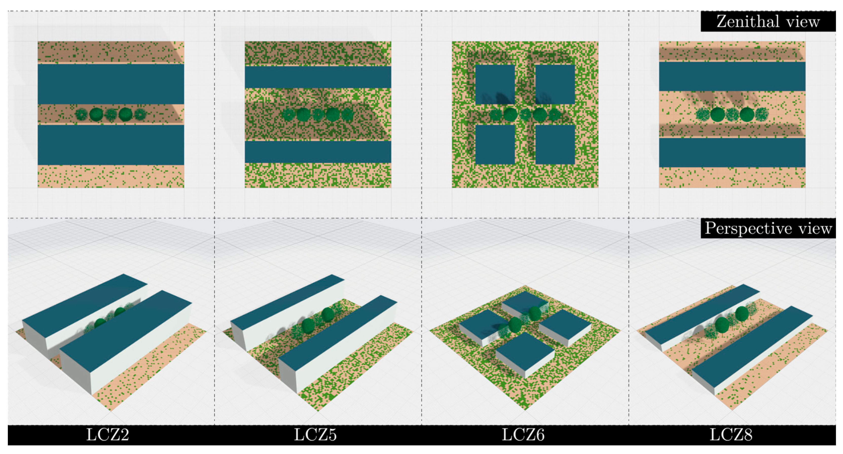
The 3D urban scenes including trees were defined using the local climate zone (LCZ) taxonomy [43,54]. Four LCZ types were selected from the most dominant LCZ built-cover types encountered in European cities with more than 100,000 inhabitants [55]: LCZ 2 (Compact Midrise), LCZ 5 (Open Midrise), LCZ 6 (Open Low-rise), and LCZ 8 (Large Low-rise). Three LCZ parameters were used to build contrasting urban scenes: height of roughness elements, which is the mean height of the buildings; aspect ratio, calculated as the height of roughness elements divided by the width of the urban canyon; and fraction of area in buildings, which is the percentage of the ground surface occupied by buildings. Their values (Table 3) did not vary during the simulations.
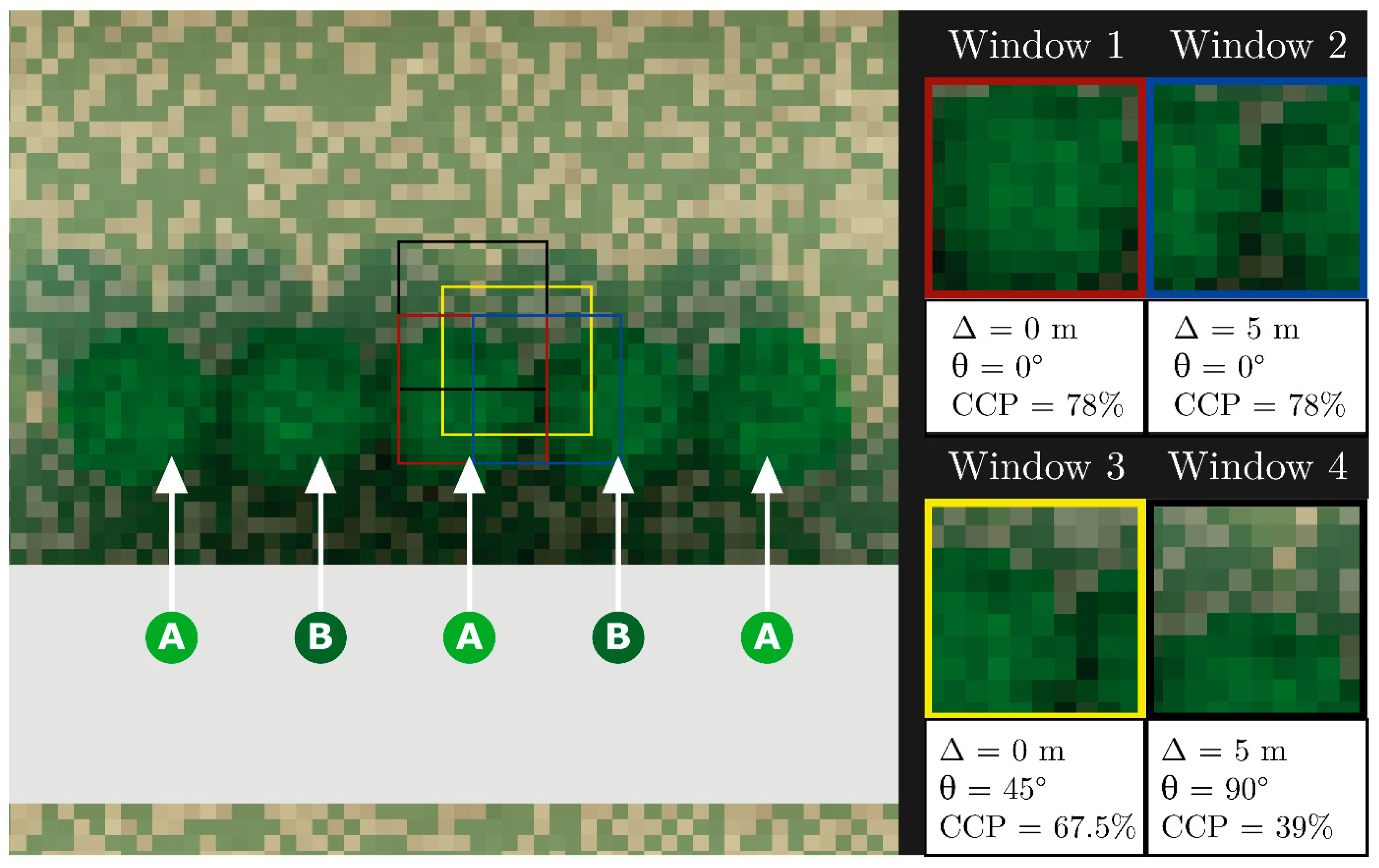
Only deciduous tree species were modelled. We defined a 3D tree model (reference tree) with a tree height of 15 m, crown height of 11 m, and trunk diameter of 0.4 m, based on statistical analysis of the urban tree database of the Lyon Metropolitan Area (France) (https://data.grandlyon.com/jeux-de-donnees/arbres-alignement-metropole-lyon/info, accessed on 17 July 2024). The 3D tree was modelled with an ellipsoid crown and a cylindrical trunk with branches. This simplistic representation was already used for other studies in urban and forest contexts [56]. To consider alignment heterogeneity, we created an alignment of five trees that contained two profiles of tree functional traits. Specifically, the central tree and the two trees at the ends of the alignment had one profile of optical and biophysical traits (profile A), while the other two trees had the other profile (profile B) (Figure 3 and Figure 4). The 3D urban scenes were generated using R, and the final 3D objects (.obj format) were then input into DART.

2.4.2. DART Parametrization and Simulation

Although DART includes dozens of tunable parameters, 32 parameters were used to simulate S2 images (Table 4). See Appendix A for details of these parameters. They included 12 tree-endogenous and 20 tree-exogenous parameters that have direct or indirect influence, respectively, on simulated tree canopy reflectance. Whereas some parameters (15) were fixed, others (17) varied according to predefined values/ranges and distributions. For the purpose of generalization, the min and max bounds for the leaf traits were determined with reference to the literature [57,58].
DART inputs were created from the variable parameters (Table 4) using a design of experiment (DOE) computational approach based on a Latin hypercube sampling (Python v3.9 library OpenTurns v1.34 [59]). A total of 80,000 simulations were performed (i.e., 20,000 per LCZ). Thus, 80,000 coordinate points [X1, …, Xp] were generated, where p is the number of parameters, to cover the p-dimensional space as well as possible. For continuous variable parameters (type = V in Table 4), values were generated using a uniform distribution.
DART was configured to generate orthorectified images with a size of 100 m × 100 m, and a spatial resolution of 1 m. The images were generated according to the S2 spectral and geometrical (view angles) characteristics. Specifically, only the 10 m (VIS and PIR) and 20 m (RE, SWIR) bands were simulated, and central wavelengths and bandwidths were defined based on characteristics of the S2 MSI sensor. Zenithal and azimuthal angles were set to the mean S2 view angles: 3° (with zenith = 0°) and 180° (with north = 0°), respectively. As the synthetic S2 images were initially simulated at 1 m resolution, we used a method based on extraction windows to extract pixel spectral values, considering the 10 m and 20 m spatial resolutions of S2 (see Section 2.4.3). DART version 5.8.10v1259 was used.

2.4.3. Spatial Window Extraction

The simulated images were generated at a spatial resolution of 1 m, which represented interactions among elements of the 3D scenes more precisely. We then aggregated spectral values at 10 m (B02, B03, B04, and B08) and 20 m resolution (B05, B06, B07, B8A, B11, and B12) using four pair-extraction windows of 10 × 10 and 20 × 20 m (Figure 4): one tree-centred window and three windows shifted by 5 m at 0°, 45°, and 90° with respect to the centre of the tree-canopy in the direction of the tree alignment. The 20 × 20 m windows were configured so that their lower left quarter corresponded to the associated 10 × 10 m window. This extraction-window method was applied to consider S2 pixel heterogeneity (mixed pixels), geolocation uncertainty, and urban conditions. This approach allowed a wide range of pixel compositions to be considered, with different proportions of canopy and shadow in the pixel, as well as pixels that overlapped two trees. In terms of computational efficiency, it allowed a diverse set of pixels to be obtained from a single simulated image, while decreasing the total number of simulations and simplifying parametrization.

2.5. Dataset Configuration

2.5.1. Environmental Feature Extraction

Contextual information at the pixel scale was included as three EFs in the RFR and GPR models:
  • Green proportion (Pgreen): the percentage of the pixel covered by underlying vegetation, which strongly influences reflectance when the tree canopy does not cover the entire pixel and/or the tree has low LAI;
  • Shadow proportion (Pshadow): the percentage of the pixel covered by shadow, which also strongly influences reflectance, particularly of one near-infrared S2 band (B08) with solar angle decrease;
  • Canopy cover pixel (CCP): the percentage of the pixel covered by tree canopy, which indicates the percentage of pixel purity.
For the simulated dataset (SDS), Pgreen had already been defined as an input parameter for DART (Table 4) and thus was known at the pixel scale for each simulated image. Pshadow was calculated by DART at the pixel scale for each simulated image using a direct insolation mask. CCP was calculated at the pixel scale by intersecting the four extraction windows previously defined and the crown extent simulated by DART (Figure 4). Depending on the window and crown diameter, CCP ranged from 39% (window 4 with a 10 m-diameter crown) to 95% (window 1 with a 12 m-diameter crown).
For the real dataset (RDS), EFs were calculated using different methods than those used for the SDS. First, we considered a spatial reference grid (S2 grid) that corresponded to S2 images at 10 m resolution, then EFs were calculated as follow:
  • Pgreen was calculated at the pixel scale by intersecting the S2 grid and the grass-extent layer;
  • Pshadow was calculated using a raster layer of potential direct incoming solar radiation (kWh/m2) at 1 m resolution derived from the DSM using the Potential Incoming Solar Radiation algorithm (Terrain Analysis; Lighting, Visibility) in SAGA software v7.8.2 [60]. Pixels with > 0 kWh/m2 were classified as non-shadow (0), while those with 0 kWh/m2 were classified as shadow. This layer was then aggregated to the S2 grid resolution (10 m);
  • For CCP calculation, the S2 grid and the tree-crown extent were spatially intersected. Finally, CCP was calculated at the pixel scale based on this spatial intersection.

2.5.2. Spectral Feature Extraction

Spectral features were extracted on specific spatial locations depending on the dataset. For the RDS, pixels with CCP < 35% were removed, as this value was close to the minimum CCP of the SDS (39%); the remaining pixels were considered pixels of interest. Spectral features were then extracted from the pixels of interest for the RDS and in the windows for SDS, and 18 vegetation indices correlated with LCC and LAI according to the literature were calculated for both datasets (Table 5).

2.5.3. Spatial Allocation for Field-Satellite Data Matching

To match field and satellite data, we applied two spatial allocation (SA) methods that intersected pixels and crown areas: one at the tree scale and one at the pixel scale. The former simply allocated the field measurements of LCC, LAI, and CCC of the dominant tree in a given pixel to that pixel (LAItree, LCCtree, and CCCtree, respectively). The pixel-scale method considered the percentage of trees at the pixel scale by weighting the field measurements of LCC, LAI, and CCC of the tree(s) by their crown area in the pixel (LAIpix, LCCpix, and CCCpix, respectively).
Both methods were applied to the SDS and RDS. Before doing so, tree LAD (m²/m3) was converted into LAI (m2/m2), as the in situ LAI-2200 measurements and DART input values for a given tree were LAD. This step required knowing geometric properties of the trees, which were derived from the auxiliary data for real trees or from DART input parameters for simulated trees (Table 6). This step was based on two simplifying assumptions: (i) crown height equals 2/3 of the tree height (i.e., live crown ratio [79,80,81], and (ii) the tree crown can be considered an ellipsoid, which can be used to calculate its volume.
Both SA methods intersected crown area and the extraction window for SDS or the S2 grid for RDS to calculate five properties (Table 7): pixel area, intersection area between a given tree and a pixel (when several trees intersected a pixel, the intersection area of each tree was calculated), total canopy area of the pixel, percentage of canopy cover of the pixel, and the percentage of canopy in the pixel for a given tree.
For the tree-scale method, LCCtree equalled the value measured in situ or the DART input parameter, LAItree was calculated from LAD (Table 6), and CCCtree equalled LAItree × LCCtree (Table 8). For the pixel-scale method, the vegetation traits for each pixel were calculated using equations (Table 8).

2.6. Machine Learning Regression Algorithms: Building Strategy and Training

For each of the three vegetation traits (LCC, LAI, and CCC), we built a total of 24 regression models depending on different configurations defined by three components: (i) the type of MLRA (RFR or GPR), (ii) the exclusion or inclusion of EFs (models trained using only spectral features or combining these spectral features with the three EFs (CCP, Pgreen, and Pshadow)), and (iii) the SA method (tree scale or pixel scale).
RFR and GPR have been widely used to estimate LAI and LCC from S2 data using hybrid inversion approaches with PROSAIL [29,82], INFORM [27], and DART [42] models. Non-parametric MLRAs such as RFR and GPR provide faster and more accurate estimates than simple parametric MLRAs do [23]. Their ability to capture non-linear relationships and interactions among variables makes them suitable for simulating complex datasets. RFR is an ensemble-learning algorithm that combines the predictions of several decision trees built from bootstrap data samples. This method, which can capture complex relationships between explanatory and interaction features, addresses overfitting problems effectively while maintaining high prediction accuracy. GPR uses Bayesian inference and a pre-set covariance kernel function that is optimized to fit the data. The kernels provide the expected correlation between different observations. In this study, the SDS and RDS included spectral, derived (vegetation indices), and contextual features. We used a radial basis function as the kernel to train GPR.
To identify an optimal set of input spectral features to use to train the models, a Pearson correlation matrix was calculated, and, when two features were strongly correlated (i.e., r > 0.95), the feature with the largest mean absolute correlation was removed. This step aimed to improve model interpretability and performance by removing redundant features.
Next, for each target variable and both SA methods (i.e., LCCtree, LCCpix, LAItree, LAIpix, CCCtree, and CCCpix), recursive feature elimination (RFE) was applied, which iteratively removed less informative features by calculating variable importance based on random forests. Backward selection of features was based on the root mean square error (RMSE), which was calculated using a cross-validation procedure with 10 folds and two repeats. RFE was applied to each target variable, and the feature set with the lowest RMSE (Figure 5) was used for model training. For RFR models, hyperparameter tuning was performed using a grid-search approach with an RMSE cost function. Two parameters were used for the grid search: the number of trees {100, 200, …, 1000} and the number of random features selected at each division n 4 , n 3 , n 2 (where n is the number of training features). The parameter combination with the lowest RMSE was used for model training. Overall, 24 models were trained and evaluated (three target variables × eight configurations per target variable).

2.7. Validation

All models were cross-validated using a k-fold strategy, with k = 10. Once models were trained with the SDS, they were applied to the RDS and validated using field measurements in the RDS. The minimum, mean, and maximum values of the vegetation traits included the RDS, which were determined based on the two SA methods and in situ measurements, are presented in Table 9.
Five metrics were used to assess the performance of the regression models:
  • Coefficient of determination (R2): The coefficient of determination measures the proportion of the variance in the dependent variable that is explained by the regression model. It ranges from 0 to 1, where 1 indicates a perfect fit of the model to the observed data.
R 2 ( O b s , P r e d ) = 1 i = 1 n P r e d i O b s i ² i = 1 n P r e d i P r e d i ¯ ²
  • Root mean squared error (RMSE): RMSE is a measure of model accuracy that calculates the square root of the mean of the squares of the differences between predictions and observations, thus indicating the mean deviation between them.
R M S E ( O b s , P r e d ) = 1 n i = 1 n P r e d i O b s i ²
  • Symmetric mean absolute percentage error (SMAPE): SMAPE equals the percentage difference between predictions and observations while accounting for their scales. In this study, it provided an intuitive interpretation and allowed model performances for the three vegetation traits to be compared.
S M A P E ( O b s , P r e d ) = 100 n i = 1 n P r e d i O b s i O b s i + P r e d i · 0.5
  • Bias: Bias equals the mean difference between predictions and observations, which indicates a model’s tendency to overestimate or underestimate the dependent variable.
B i a s ( O b s , P r e d ) = 1 n i = 1 n ( O b s i P r e d i )
  • Bias standard deviation (BSD): The standard deviation of the bias measures the distribution of prediction errors around the mean bias, which indicates the variability in differences between predictions and observations.
B S D ( O b s , P r e d ) = 1 n i = 1 n ( O b s i P r e d i ) B i a s ²
For Equations (2)–(6), Obs is the observed value of the target variable, Pred is the predicted value of the target variable, and n is the total number of samples in the RDS.
Finally, temporal metrics were calculated to assess the temporal consistency between estimated and observed values. Temporal consistency ensures that observed changes or trends in predicted vegetation traits reflect real phenomena rather than artefacts introduced by inconsistencies in data acquisition or processing [83]. This is particularly important in the context of vegetation monitoring, when trends and/or temporal anomalies derived from image time-series are most often more relevant than information obtained from single-date observations [22,84]
The LCC, LAI, and CCC time series were estimated for each pixel using the best models (according to the metrics used). For each pixel, the estimated series were compared to the observed series. Three temporal similarity metrics available in the R package TSclust [85] were used:
  • dEUCL, based on the Euclidean distance between values observed at the same points in time
  • dCOR, based on Pearson correlation between the two series [86]
  • dCORT, based on temporal correlation between the two series, used to include both conventional measures for the proximity of observations and temporal correlation to estimate the proximity behaviour and dynamic [87].

3. Results

3.1. Accuracy of LCC, LAI, and CCC Estimation Using the Simulated Dataset

Values of metrics calculated for all configurations are shown in Table 10. Cross-validation scatterplots are shown in Appendix B.
For LCC estimation, R2 ranged from 0.68–0.82. SA influenced LCC accuracy the most, with R2 of 0.67–0.71 for tree-scale SA and 0.77–0.82 for pixel-scale SA. The two MLRAs performed similarly, with slightly higher R2 and lower RMSE for RFR (R2 = 0.80–0.82 and RMSE = 4.16–4.34 μg/cm2) than for GPR (R2 = 0.77–0.79 and RMSE = 4.38–4.57 μg/cm2). Nevertheless, GPR had a smaller bias than RFR. Inclusion of EFs did not influence LCC estimation significantly, with models that did so having only slightly better evaluation metrics. Overall, the best model for estimating LCC was RFR with pixel-scale SA and inclusion of EFs, which had high accuracy during cross-validation.
For LAI estimation, R2 ranged from 0.13–0.56. To a greater extent than that for LCC models, SA influenced accuracy the most, with R2 of 0.13–0.35 for tree-scale SA and 0.37–0.52 for pixel-scale SA. The type of MLRA had a pattern similar to that for LCC models, with RFR having slightly higher R2, lower RMSE, but smaller bias than those for GPR. Unlike for LCC models, inclusion of EFs influenced LAI estimation strongly, leading the RFR model with pixel-scale SA and inclusion of EFs to have R2 0.17 higher than that of the same configuration but without EFs.
CCC estimation followed the same pattern as those for LCC and LAI estimation. The best model for estimating CCC was RFR with pixel-scale SA and inclusion of EFs (R2 = 0.68 and RMSE = 36.39 μg/m2).

3.2. Accuracy of LCC, LAI, and CCC Estimation Using the Real Dataset

3.2.1. Overall Accuracy Assessment and Consistency between Cross-Validation and Validation Using the Real Dataset

For LCC accuracy, R2 ranged from 0.24–0.33 (Table 11). SA influenced LCC accuracy slightly, with R2 of 0.24–0.3 for tree-scale SA and 0.24–0.33 for pixel-scale SA. RFR outperformed GPR (SMAPE = 16% and 21%, respectively). Inclusion of EFs did not influence LCC estimation significantly, with models that did so having only a small decrease in bias. Similar to the results obtained using cross-validation, the LCC model with the best performance was RFR with pixel-scale SA and inclusion of EFs.
For LAI accuracy, SA had a significant influence: the four models with tree-scale SA had R2 close to 0, unlike those with pixel-scale SA, for which R2 ranged from 0.12–0.29. For the MLRAs, GPR did not achieve SMAPE < 50%, unlike RFR, which had SMAPE of 47% and 49%. Unlike for the LCC models, inclusion of EFs improved LAI accuracy. Comparing the two RFR models with the pixel-scale SA, the one that included EFs had higher accuracy than the one that excluded them, with a higher R2 (0.29 vs. 0.22, respectively), lower RMSE (1.18 vs. 1.30 m2/m2, respectively) and lower bias (−0.58 vs. −0.69, respectively).
For CCC accuracy, SA also had a significant influence: models with pixel-scale SA had much higher R2 (0.27–0.46) than those with tree-scale SA (0.12–0.16). Similarly, RMSE was lower with pixel-scale SA (36–51 μg/m2) than with tree-scale SA (49–57 μg/m2), but the bias was much larger with pixel-scale SA. The RFR model with inclusion of EFs outperformed the other models according to all metrics.

3.2.2. Accuracy of LCC, LAI, and CCC Estimation by Tree Species

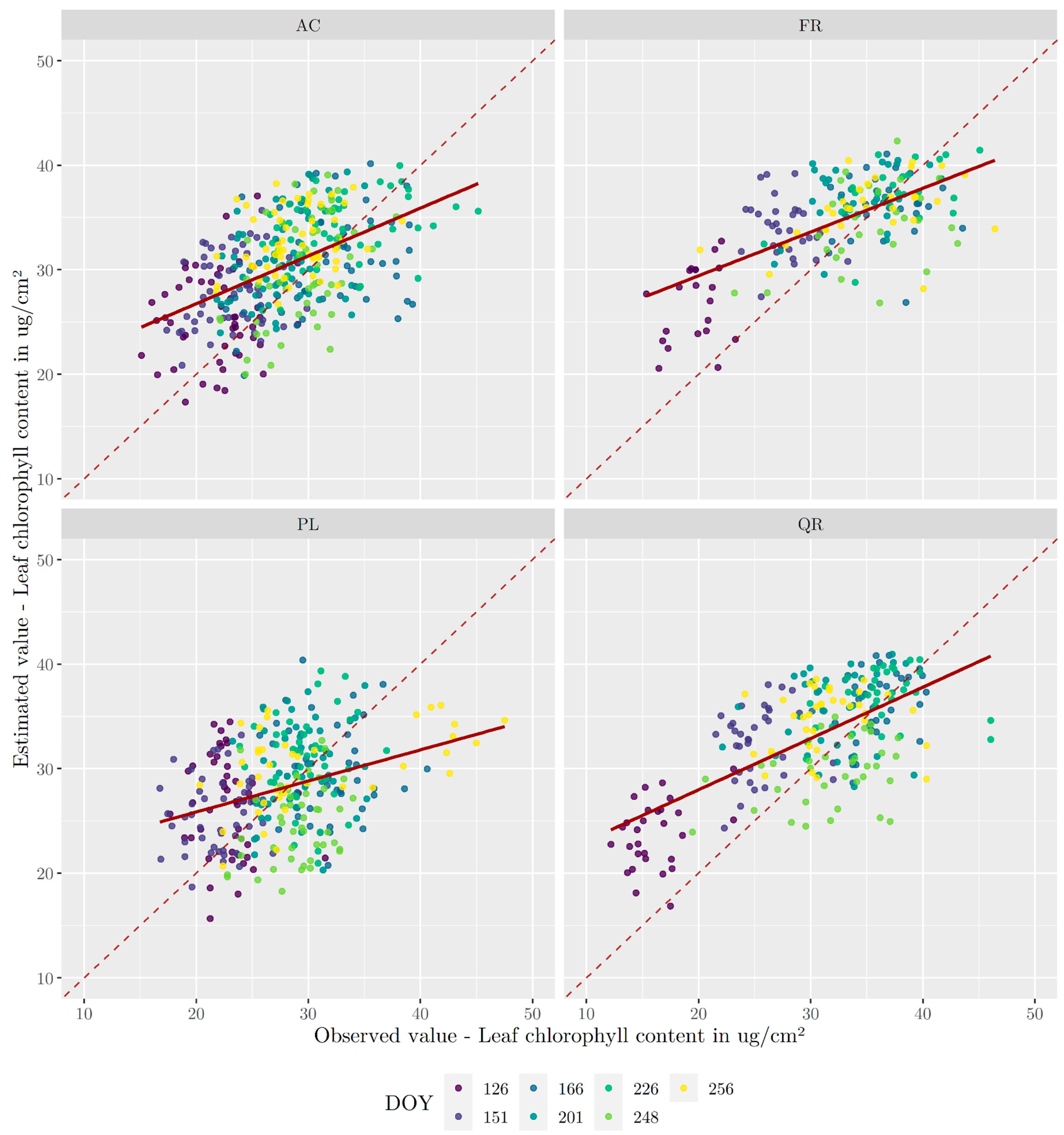
Using the best model for each target variable, we estimated the target values by tree species. The model used to estimate LCC showed high tree-species dependence, with R2 ranging from 0.11 for PL to 0.45 for QR (Table 12).
FR and QR followed a similar pattern for LCC (Figure 6), with overestimation from low to median LCC (10–30 µg/cm2). Conversely, LCC patterns for AC and PL were more scattered. We also found a phenological trend, with LCC lower for early dates (i.e., day of the year (DOY) 126 and 166) than for later dates.
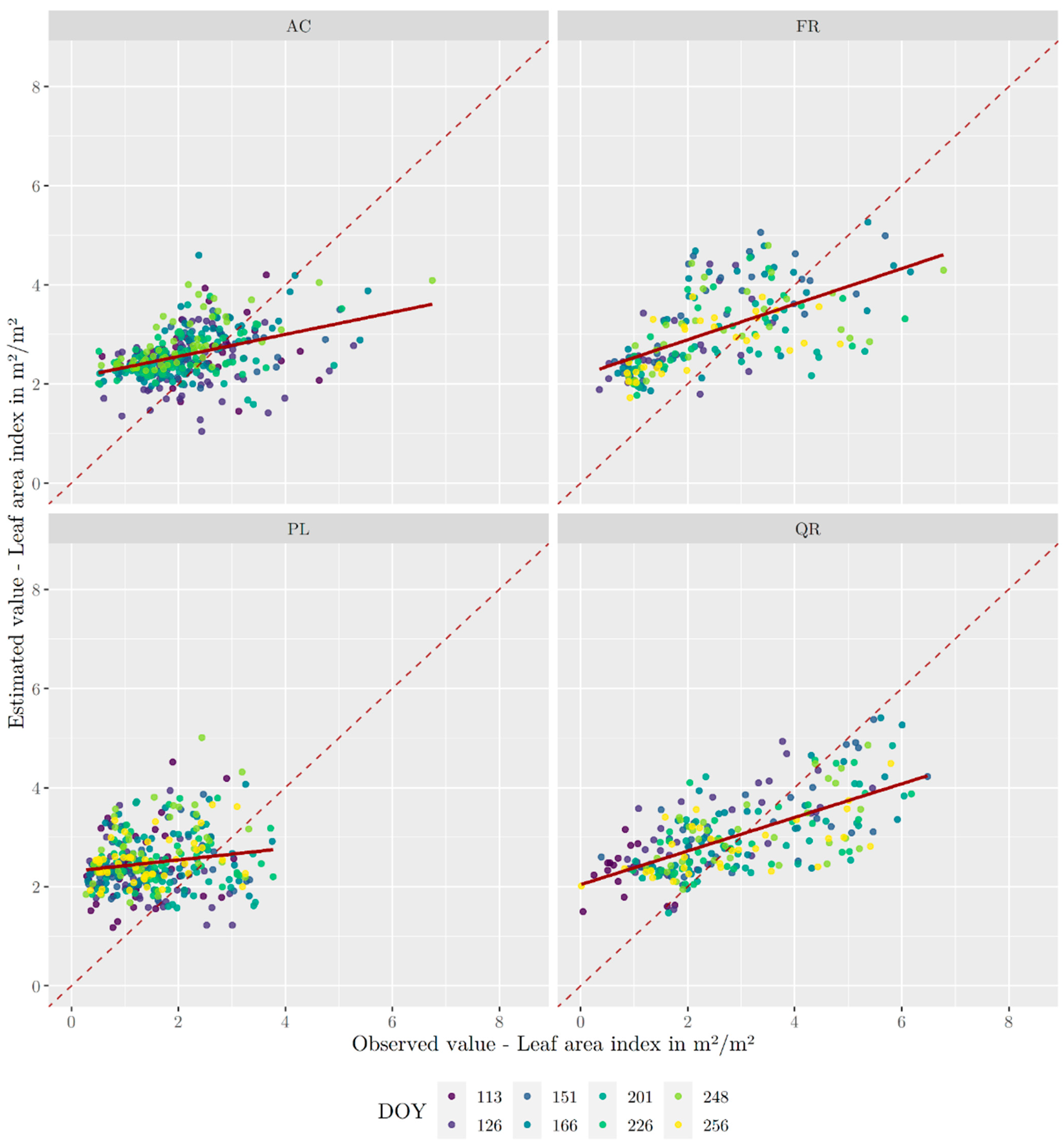
The model used to estimate LAI was also species-dependent, with R2 ranging from near-zero for PL (0.03) to moderate for QR (0.43). A similar pattern was found for the four species, with overestimation of low LAI (0–2), and few LAI < 2 being estimated. The best performances were observed for QR and FR, but with a positive bias (i.e., overestimation) for LAI of 0–2.5 and a negative bias for LAI of 2.5–6.0 (Figure 7).
CCC estimation followed a pattern similar to that of LAI, with low R2 for PL and AC (0.10 and 0.28, respectively) and clustering of estimated values (Figure 8). Performances were better for QR and FR (R2 of 0.55 and 0.50, respectively), which followed a distinctive pattern with overestimated low CCC and underestimated high CCC, and an inflection point around 100 µg/m2.
Overall, for the three target variables, PL and AC followed a similar pattern, while FR and QR followed another similar pattern.

3.3. Consistency between Estimated and Observed Time Series

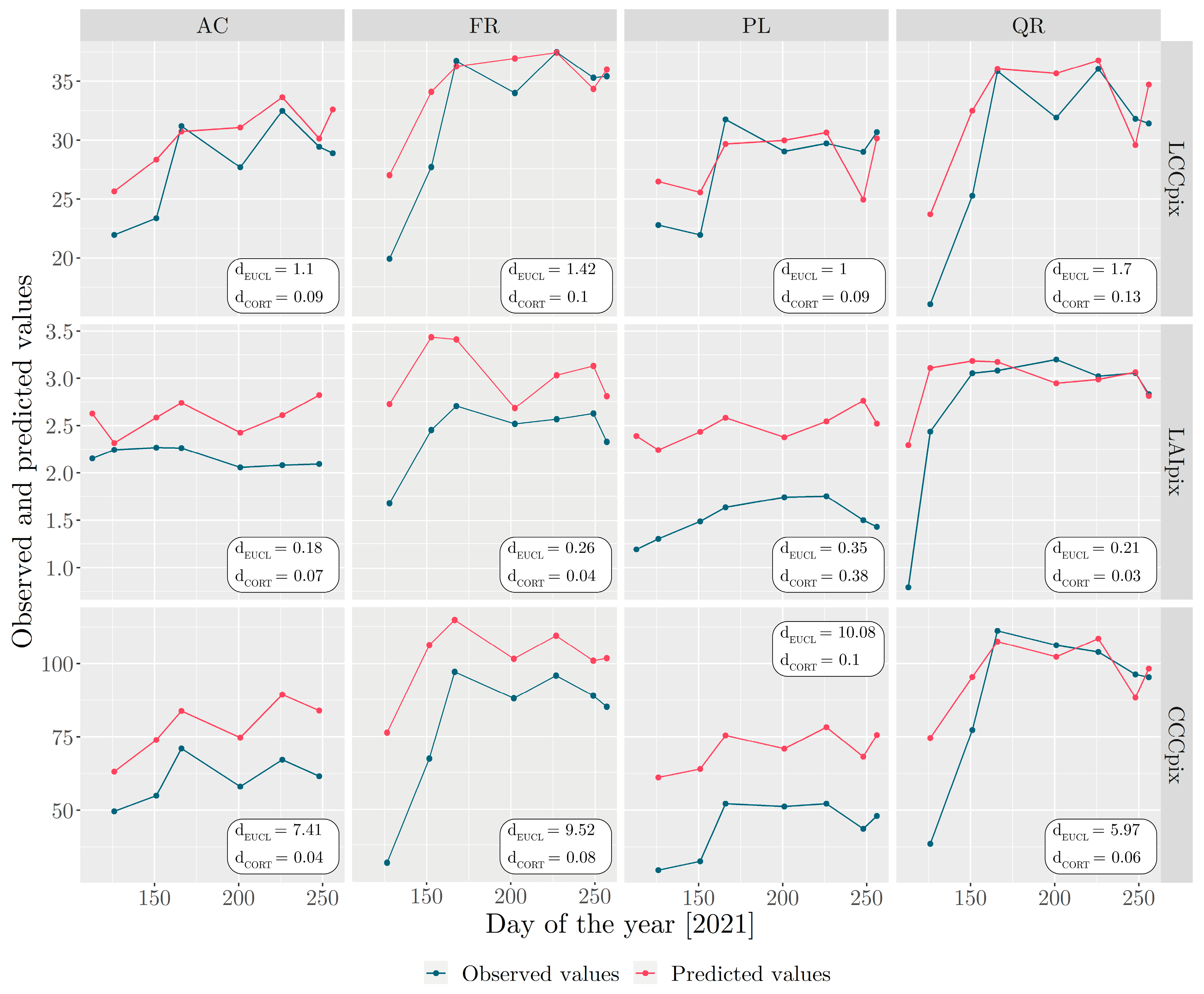
For each target variable and species, we examined the mean time series (Figure 9) and distribution of temporal metric values (Figure 10) to assess the temporal consistency between estimated and observed series. High adequacy was observed between estimated and observed LCC time series according to dEUCL and dCORT (Figure 9). There were no significant differences among the four species. In particular, the observed LCC time series decreased from DOY 166 to 201 and then increased from DOY 201 to 226. This pattern was also found, to a lesser extent, in the estimated LCC time series for AC and QR. For LAI, the estimated time series differed much more from the observed time series. Temporal trends were observed for FR (dCORT = 0.04) and QR (dCORT = 0.03). AC and PL showed differences between the estimated and observed time series. Values of dEUCL were particularly high for PL. The estimated and observed CCC time series showed high adequacy, with similar temporal trends for AC and FR. However, a strong positive bias in the estimated CCC time series was observed for AC, FR, and PL (dEUCL = 7.41, 9.52, and 10.08, respectively).

4. Discussion

Results highlighted two main points: (i) evaluating accuracy using cross-validation revealed that (i) pixel-scale SA estimated all target variables better than tree-scale SA, (ii) including EFs in model training improved model performance (especially for LAI and CCC), and (iii) RFR gave slightly better estimates than GPR. Comparing the three target variables, the models had good accuracy for LCC estimation and moderate accuracy for CCC and LAI estimation (SMAPE = 11%, 29%, and 30%, respectively); (ii) the highest R2 obtained using the RDS was 0.46 for CCC, 0.33 for LCC, and 0.29 for LAI. We reached the same conclusions using the RDS as when using SDS: for all three target variables, the best configuration for the model was RFR with pixel-scale SA and inclusion of EFs. However, the models had lower overall accuracy when using the RDS than when using SDS.

4.1. Overall Performance of Vegetation Trait Estimation

The best performances for LCC estimation in the study were R2 of 0.33 with high variability among species, R2 ranging from 0.11 (PL) to 0.45 (QR), and RMSE of 5.64 µg/cm2. Although LCC, LAI, and CCC of urban trees had never been estimated using S2 images, LCC has been estimated using a non-species-specific model for urban trees based on hyperspectral images at 1 m spatial resolution in an urban area that contained PL, with R2 of 0.77 [88]. Another study that used species-specific models in an urban area based on hyperspectral images at 2 m spatial resolution [89] had R2 of 0.33 and 0.62, for AC and PL, respectively.
The combination of S2 data with hybrid inversion models based on PROSAIL has been successfully used to estimate LAI and LCC with high accuracy. A study conducted on tree plantations showed R2 values above 0.8 for LAI estimation [36], and another study including seven vegetation types (crops, forests, wetlands, …) showed an R2 value of 0.62 for LCC estimation [37]. However, these models did not take into account the complexity of urban environments.
Among studies that estimated vegetation traits using S2 imagery, the most similar case studies were based on forest canopies or sparsely wooded areas and used hybrid inversion methods based on DART or INFORM. Comparing the best model in the present study (RFR with pixel-scale SA and inclusion of EFs) to INFORM inversion for mixed forest [27], we found similar validation R2 for LCC estimation (0.33 vs. 0.34, respectively). For LAI and CCC estimation, however, the present study’s models had lower R2 than those of the other study: 0.29 vs. 0.47 and 0.46 vs. 0.65, respectively. However, in both studies, model validation using simulated datasets showed the same pattern, with very good performance for LCC, good performance for CCC, and moderate performance for LAI. Another study based on DART and based on an agricultural area with olive orchards had good performances for LAI (RMSE = 0.58 m2/m2) and LCC (RMSE = 2.5 µg/cm2) [42]. These good performances can be explained by the high detail in 3D models of the trees and prior knowledge of soil optical properties extracted from S2 pure pixels, which was not possible in the present study because it is nearly impossible to extract pure pixels of soils in urban areas from images with a spatial resolution of 10 m, and because soil composition varies greatly among pixels in urban areas.
Validation using the real dataset did not show high accuracy for estimation of vegetation traits. However, while high estimation accuracy may be needed for certain ecophysiological applications in agricultural areas, moderate accuracy may be sufficient for monitoring purposes in urban areas. There was high temporal consistency between observed and estimated vegetation traits, particularly according to the dCORT metric, which highlighted similar trends for estimated and observed values. The temporal trend in vegetation traits may be more informative than the absolute values of these traits when studying the phenology and response of vegetation to stress events [90].

4.2. DART Modelling

The DART model has been used in studies that examined various aspects of the urban environment, such as retrieving spectral signatures [91,92], assessing radiative budgets [41], investigating temperature patterns [93], and studying impacts of 3D structures on emissivity [94]. Nevertheless, to the best of our knowledge, no inversion models of vegetation traits of urban trees have been developed using DART or other RTMs. While physical approaches are inherently general and applicable in many contexts, they are limited by competing demands of model realism and inversion feasibility. A simplified approach to complex physical processes is usually required to constrain inversion in a remote sensing context [95,96]. Unlike some approaches used, mainly for calibration, that involve direct simulations with high accuracy and definition of 3D scenes, this study’s approach is more global and aims to cover a wide range of urban configurations and model pseudo-realistic urban scenes. Thus, we made several simplifications, notably to the 3D tree model. Tree structure determined the proportion of woody elements in the crown, as branch shape, length, and density can strongly influence reflectance, especially when LAI is low [50], and thus the accuracy of LAI estimation. The present study’s two simplifying assumptions (crown height equalled 2/3 of tree height and the crown was an ellipsoid) enabled us first to acquire a validation dataset using LAI-2200 measurements and a DSM—without requiring terrestrial LIDAR data, which are much more difficult to acquire—and then to aggregate these values at the pixel scale. However, the live crown ratio and crown shape may be species-specific [79], which may explain the overall moderate performance of LAI estimation and the variability in performances among tree species.

4.3. Environment Features

One key point of this study was the use of contextual information for simulation and model training. The LCZ classification system was used as a framework for the construction of pseudo-realistic urban scenes. While the four LCZ types were selected among the most dominant LCZ built-cover types encountered in European cities with more than 100,000 inhabitants, these LCZ types did not cover all the urban environments of our study site. In particular, the dense, high-rise urban centre corresponding to LCZ type 1 (“Compact high-rise”) was excluded. However, it does not affect the transferability of the models, because tree vegetation is less prevalent in this LCZ type than in the four LCZ types selected. Nevertheless, many tree-exogenous parameters were used for the DART simulations, including differences in LCZ type, material type, contextual parameter, and underlying vegetation. However, using a large number of parameters can increase the probability of encountering ill-posed problems, when nearly identical spectra may correspond to different combinations of model input parameters [97,98]. To mitigate these issues and improve model performance, many studies developed regularization strategies, which incorporate supplementary information and adopt constrained inversion methods [99,100,101,102]. However, these strategies often rely on adjusting RTM input parameters to better match the magnitude of in situ vegetation traits or contextual features such as soil spectra. While these approaches can improve performance, they may decrease the generality of the resulting inversion models.
In the present study, contextual input information was summarized into three EFs at the pixel scale (CCP, Pshadow, and Pgreen). The strategy was to consider using these features to train the models (as they interact with spectral features) rather than to filter or restrict the simulated data so that their characteristics match those of the RDS. However, building the model in this way required obtaining real data that corresponded to these features to apply the inversion model. Vegetation cover and DSM data are now widely available at the scale of major European cities via Open Data city portals, OpenStreetMap, the Copernicus portal, and Google Earth Engine, including a highly accurate, Europe-wide DSM [103].
The models that included EFs performed better for all three vegetation traits, especially LAI. In the machine-learning approach, EFs were considered interaction features, as they were not directly correlated with vegetation traits, although they strongly influenced spectral features. One advantage of RFR is its ability to exploit interaction effects between the features effectively [104]. Including these three EFs allowed a wider range of pixels of interest to be considered (first for the validation dataset, and then for mapping), without having to filter pure pixels, pixels in shadow, or pixels with underlying vegetation, which makes this approach particularly efficient for urban areas.

4.4. Spatial Allocation

The models’ performances showed the importance of the SA method used. Correspondence between the spatial coverage of the objects of interest (i.e., trees) and satellite images is essential for model validation, particularly in an urban environment in which the dimensions of the objects of interest are similar to those of the pixel. Correspondence is not a problem when the canopy studied is spatially homogeneous and in situ measurements can be performed in a homogeneous way. In many studies, in situ measurements are made at the plot scale, using a square that is usually larger than the resolution of the satellite image. For example, using S2 imagery, Ali et al. [27] and Brown et al. [26] took measurements in plots with 30 and 40 m sides, respectively. In sparse canopy, methods need to be adapted to match satellite and in situ data. For example, Makhloufi et al. [42] measured the LAI of isolated trees and then related the measurements to the area of a plot to estimate total LAI at the plot scale. We followed a similar approach, which considered the presence of several trees and their canopy cover in the pixel. This approach was able to address details of urban vegetation layout, such as street tree alignments. Although overall performance was moderate, the fact that pixel-scale models outperformed tree-scale models demonstrated the benefits of this approach.

5. Conclusions

This study examined an innovative approach for estimating vegetation traits LCC, LAI, and CCC of urban trees using S2 imagery and a hybrid inversion method based on the DART model. Combining DART with RFR and GPR effectively captured the complexity and heterogeneity of urban environments. One major contribution of this study is the inclusion of EFs such as CCP, Pshadow, and Pgreen in the regression models, which significantly improved model performance, particularly for estimating LAI and CCC. The study also showed that pixel-scale SA provided more accurate results for all vegetation traits, highlighting the need for precise spatial matching between in situ measurements and satellite data in urban areas. Species-specific analysis revealed variability in model performance, with certain species showing higher accuracy. Despite moderate overall performance, the models showed strong temporal consistency, particularly for LCC, making them valuable for monitoring intra-annual urban tree dynamics. This research highlights the potential of freely available Sentinel-2 imagery for monitoring and managing urban trees. Future research will focus on species-specific modelling, extending the method to different urban contexts, and exploring the inclusion of additional environment variables to further improve model performance and applicability.

Author Contributions

T.L.S.: Conceptualization, visualization, methodology, investigation, writing—original draft; J.N.: Conceptualization, methodology, investigation, project administration, funding acquisition, supervision; L.H.-M.: Supervision, writing—review and editing; K.A.: Conceptualization, methodology, investigation, supervision, writing—review and editing. All authors have read and agreed to the published version of the manuscript.

Funding

This study was supported by Rennes Métropole and the Association Nationale de la Recherche et de la Technologie (ASTRESS project and grant no. 2021/0301).

Data Availability Statement

Field survey data for LCC and LAI measurement are available at https://zenodo.org/records/12751353 (accessed on 17 July 2024).

Conflicts of Interest

The authors declare no conflicts of interest.

Appendix A. Detailed Description of DART Input Parameters

Appendix A.1. Tree-Exogenous Parameters

Appendix A.1.1. Sensor Settings, Direction Input Parameter, and Atmosphere

The illumination of the scene is important, as it determines the distance of the shadow cast by the buildings (and the energy balance of the scene). These conditions change throughout the year, characterized by a change in the solar incidence angles (zenith and azimuth). To reproduce this change, the date can be set in DART (which will determine the solar angles for a given latitude and longitude) and then changed. We considered dates from 15 March to 15 November, which coincides with the vegetative period of the trees. Concerning parameters for the atmosphere, urban areas have a specific atmosphere because the concentration of housing and industry produces large amounts of emissions that influence the composition of the atmosphere and aerosols. Images acquired in urban areas are therefore influenced more by absorption and scattering, mainly in the visible and near-infrared wavelengths. The DART model can use the USSTD76 atmospheric model [105] to reproduce the atmospheric influence on the signal. Optical properties of aerosols can also be set; this study used an urban aerosol with a constant multiplier of one for the optical depth of aerosols.

Appendix A.1.2. Spectral Library

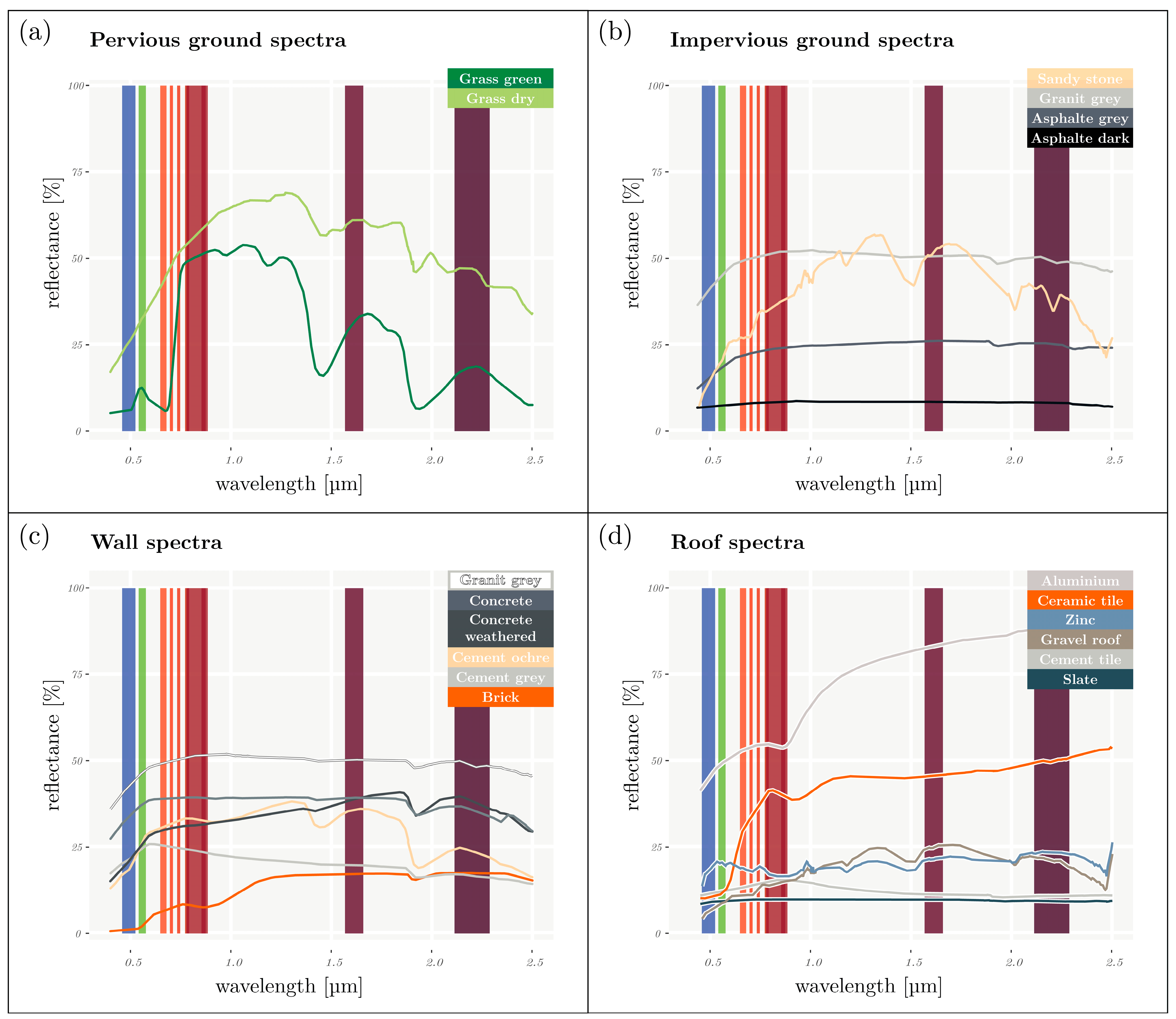
One characteristic of the urban environment is the variety of materials, most of which are human-made or mineral, such as rough stone (e.g., sandstone, limestone), granite, asphalt, cement, concrete, brick, shingle, slate, red tile, and glass, or even metals, such as steel and zinc. Each material has specific spectral signatures due to its intrinsic physical and chemical composition that will influence the land-surface radiation balance in the scene, as well as the reflectance of the pixel analyzed. Due to the geometric configuration of the four LCZs selected and the simplified 3D representations of the buildings, and to reproduce plausible contexts that represented a broad range of materials, four classes were considered: roofs, walls, impermeable ground, and permeable ground. Each of these classes was assigned potential reflectance spectra from a DART spectral library with different levels of detail. A total of 18 spectra were retained (Figure A1).
Figure A1. Spectral library showing the four spectral categories for (a) pervious ground (n = 2), (b) impervious ground (n = 4), (c) walls (n = 6) and (d) roofs (n = 6). Each spectrum is shown with its reflectance value [%] as a function of wavelength [μm]. The vertical bands correspond to the central wavelength and width of Sentinel-2 spectral bands.
Remotesensing 16 03867 g0a1

Appendix A.1.3. Earth Scene and Tree Planting Context

The scene was set in Rennes, France, to match the real Sentinel-2 data. The scene dimensions were set to 100 × 100 m based on the scale of LCZs, and to ensure that electromagnetic interactions in the tree’s environment could actually occur. The conditions under which a tree is planted are a key factor in its development. It is important to distinguish two elements: the absolute planting conditions, which include the type of ground (e.g., soil, grass, human-made materials) at the base of the tree, and the environmental conditions (e.g., the presence of buildings, the street). The former can be classified as restricted (a ca. 1 m2 square of bare soil or grass surrounded by impermeable materials), linear (trees planted on a strip of bare soil or grass surrounded by impermeable materials), or open (trees located on extended grass or in a park) [106]. In the simulations, these conditions were reflected by the ratio of permeable to impermeable ground defined with the LCZs (Table 1). The latter can be described using three parameters: the distance from the tree to the nearest building, street orientation, and exposure (planted on the sunny or shady side of the street). These three parameters are likely to strongly influence how shade will impact the tree.

Appendix A.2. Tree-Endogenous Parameters

Appendix A.2.1. Tree Structural Parameters

Tree structural parameters were determined by analysing the tree row database of the Lyon metropolitan area, which is one of the most complete databases for France in OpenData (https://data.grandlyon.com/jeux-de-donnees/arbres-alignement-metropole-lyon/info; accessed on 17 July 2024). The database contains 50,000 records with the following geometric variables: crown height, crown diameter, total height, and trunk diameter. To build a reference profile, the database was limited to the five most common genera—Tilia, Acer, Platanus, Fraxinus, and Quercus—which agrees with urban tree databases for other European cities, and to crown diameters of 8–14 m. With these limits, mean values were calculated for tree structural parameters (Table A1). The tree was further modelled with an ellipsoid crown and a cylindrical trunk without branches.
Table A1. Structural parameters of the tree modelled in DART.
ParameterValue [m]
Tree height15
Trunk height under the crown4
Trunk height in the crown6
Trunk diameter0.4
Three parameters were variable: leaf area density (LAD), the percentage of crown holes, and leaf-angle distribution. The leaf area index (LAI) was calculated as the total leaf area of a canopy per unit area of ground, which is suitable for a tree canopy with a homogeneous height such as that of dense forests. For a single tree, LAI can be defined using the LAD, which equals the total leaf area per unit volume of canopy (i.e., the tree crown) in m2/m3. Next, a clumping factor indicates the degree of spatial aggregation of leaves in the canopy. DART can calculate the percentage of crown volume occupied by leaves. If 100% of the crown volume is occupied, the LAD is homogeneous at the crown scale and the clumping factor equals 0, but if only 50% of the crown volume is occupied, the LAD is not homogeneous at the crown scale, and leaves are artificially aggregated for a given initial LAD. We used a crown hole percentage from 0–50% as a proxy to simulate the clumping factor. Finally, the leaf angle distribution refers to the statistical distribution of the angular orientation of leaves at the scale of a tree (e.g., planophilic, plagiophilic, extremophilic, uniform). Several methods exist to estimate it, including several predefined mathematical functions. From the database available in [107], which provides leaf-inclination angles for temperate and boreal broadleaf woody species, the two most common distributions (i.e., planophile and plagiophile) for deciduous tree species were extracted.

Appendix A.2.2. Leaf Parameters

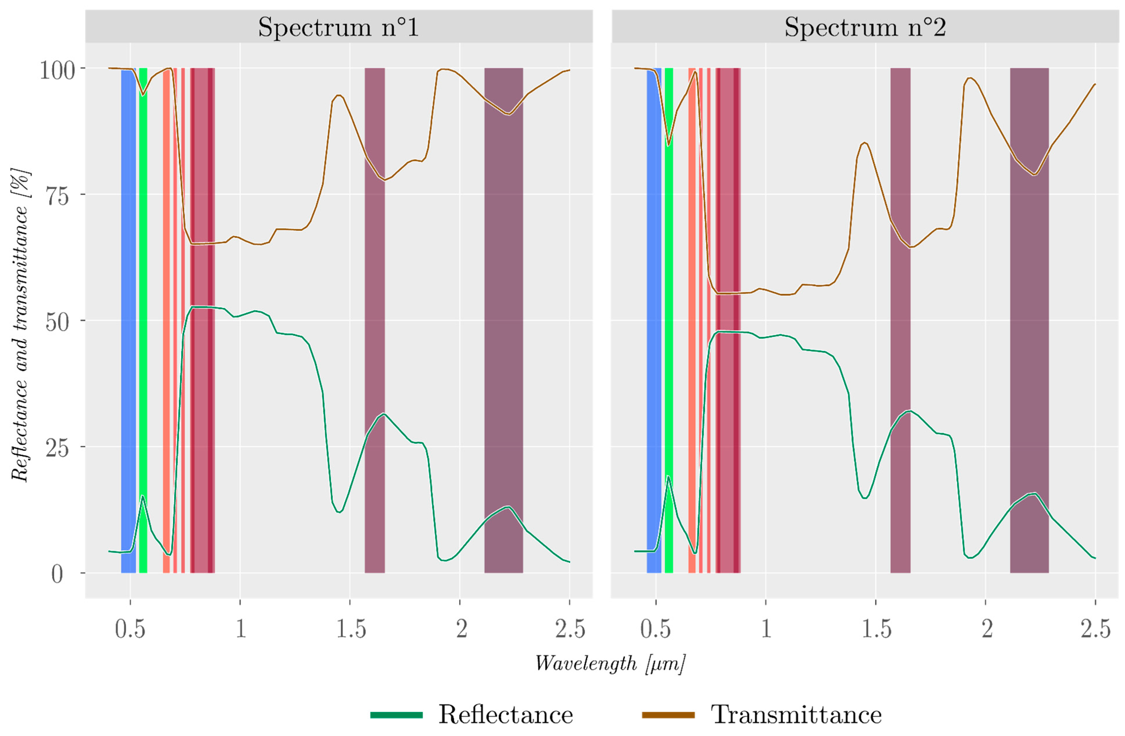
The DART model is coupled with the PROSPECT model. In this study, the PROSPECT-D version was used [31], as it can simulate the reflectance and transmittance spectra of a leaf in the spectral range of 0.4–2.5 µm (Figure A2). To simulate these spectra, the model uses seven parameters: the structure coefficient (N), chlorophyll content (Cab), carotenoid content (Car), anthocyanin content, brown pigments, equivalent water thickness (EWT), and dry matter (LMA). The simulated spectrum is then assigned to the optical properties of the tree leaves in DART.
Figure A2. Example of two leaf spectra simulated by the PROSPECT model. Spectrum 1: N = 2.3, Cab = 60, Car = 25, EWT = 0.024 and LMA = 0.018. Spectrum 2: N = 1.7, Cab = 32.5, Car = 13.75, EWT = 0.014, and LMA = 0.008. Spectra 1 and 2 correspond to maximum and median values used in the virtual experimental design, respectively. The vertical bands correspond to the central wavelength and width of Sentinel-2 spectral bands. N = structure coefficient; Cab = chlorophyll (a+b) content; Car = carotenoids; EWT = equivalent water thickness; LMA = leaf mass area.
Remotesensing 16 03867 g0a2

Appendix B. Cross-Validation Scatterplots

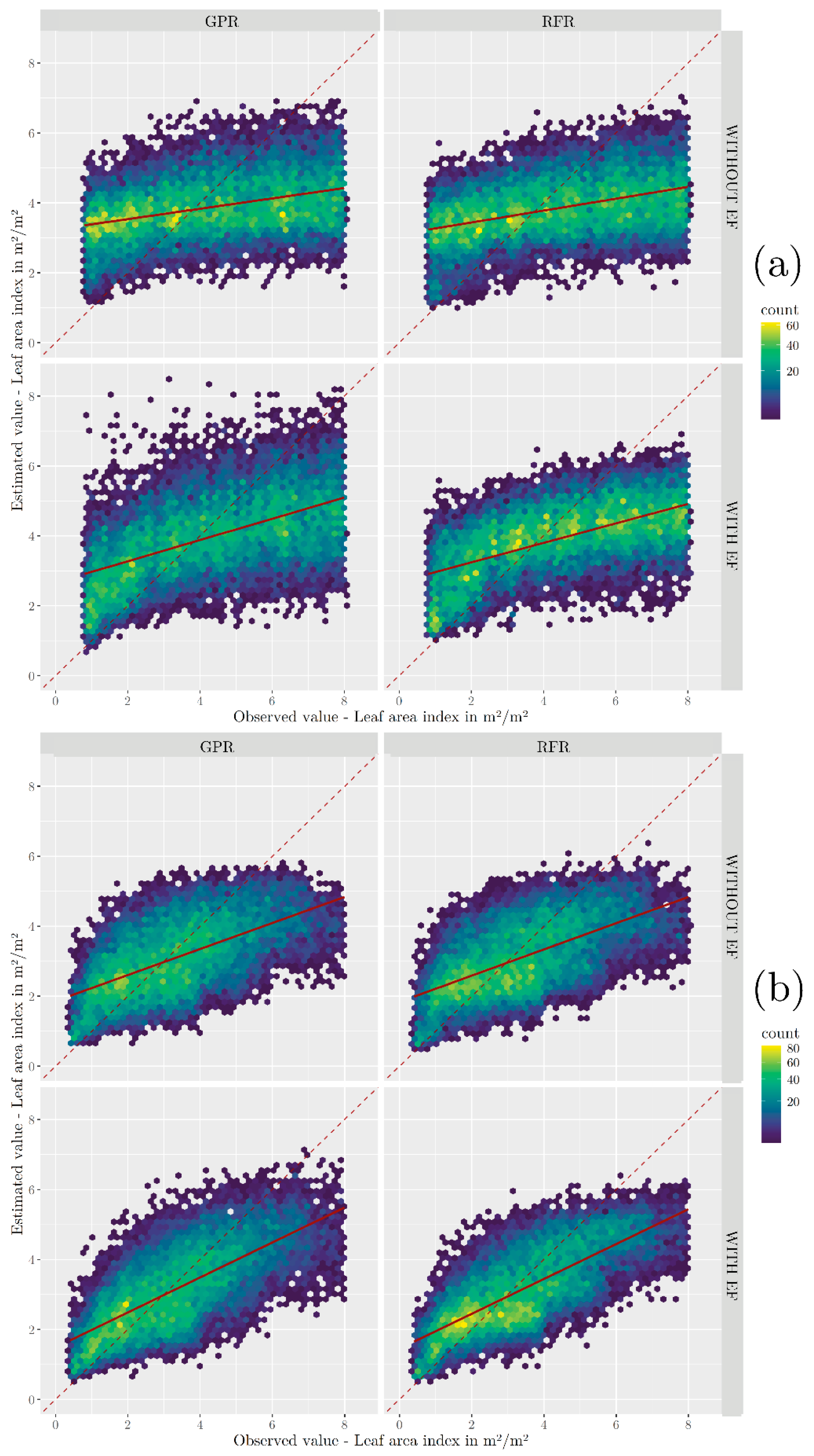
Figure A3. Cross-validation scatterplot for LCC according to the SA method (tree (a) or pixel (b)), MLRA (GPR or RFR) and inclusion of EF (with or without). LCC: leaf chlorophyll content; SA: spatial allocation; MLRA: machine learning regression algorithm; GPR: gaussian process regression; RFR: random forest regression; EF: environment feature.
Remotesensing 16 03867 g0a3
Figure A4. Cross-validation scatterplot for LAI according to the SA method (tree (a) or pixel (b)), MLRA (GPR or RFR) and inclusion of EF (with or without). LAI: leaf area index; SA: spatial allocation; MLRA: machine learning regression algorithm; GPR: gaussian process regression; RFR: random forest regression; EF: environment feature.
Remotesensing 16 03867 g0a4
Figure A5. Cross-validation scatterplot for CCC according to SA method (tree (a) or pixel (b)), MLRA (GPR or RFR) and inclusion of EF (with or without). CCC: canopy chlorophyll content; SA: spatial allocation; MLRA: machine learning regression algorithm; GPR: gaussian process regression; RFR: random forest regression; EF: environment feature.
Remotesensing 16 03867 g0a5

References

  1. Xu, F.; Yan, J.; Heremans, S.; Somers, B. Pan-European Urban Green Space Dynamics: A View from Space between 1990 and 2015. Landsc. Urban Plan. 2022, 226, 104477. [Google Scholar] [CrossRef]
  2. Bolund, P.; Hunhammar, S. Ecosystem Services in Urban Areas. Ecol. Econ. 1999, 29, 293–301. [Google Scholar] [CrossRef]
  3. Andersson-Sköld, Y.; Thorsson, S.; Rayner, D.; Lindberg, F.; Janhäll, S.; Jonsson, A.; Moback, U.; Bergman, R.; Granberg, M. An Integrated Method for Assessing Climate-Related Risks and Adaptation Alternatives in Urban Areas. Clim. Risk Manag. 2015, 7, 31–50. [Google Scholar] [CrossRef]
  4. Nowak, D.J.; Crane, D.E. Carbon Storage and Sequestration by Urban Trees in the USA. Environ. Pollut. 2002, 116, 381–389. [Google Scholar] [CrossRef]
  5. Andersson, E.; Barthel, S.; Ahrné, K. Measuring Social–Ecological Dynamics Behind the Generation of Ecosystem Services. Ecol. Appl. 2007, 17, 1267–1278. [Google Scholar] [CrossRef]
  6. Wolf, K.L.; Lam, S.T.; McKeen, J.K.; Richardson, G.R.A.; van den Bosch, M.; Bardekjian, A.C. Urban Trees and Human Health: A Scoping Review. Int. J. Environ. Res. Public Health 2020, 17, 4371. [Google Scholar] [CrossRef]
  7. Czaja, M.; Kołton, A.; Muras, P. The Complex Issue of Urban Trees—Stress Factor Accumulation and Ecological Service Possibilities. Forests 2020, 11, 932. [Google Scholar] [CrossRef]
  8. Sæbø, A.; Borzan, Ž.; Ducatillion, C.; Hatzistathis, A.; Lagerström, T.; Supuka, J.; García-Valdecantos, J.L.; Rego, F.; Van Slycken, J. The Selection of Plant Materials for Street Trees, Park Trees and Urban Woodland. In Urban Forests and Trees: A Reference Book; Konijnendijk, C., Nilsson, K., Randrup, T., Schipperijn, J., Eds.; Springer: Berlin/Heidelberg, Germany, 2005; pp. 257–280. ISBN 978-3-540-27684-5. [Google Scholar]
  9. Ma, B.; Hauer, R.J.; Östberg, J.; Koeser, A.K.; Wei, H.; Xu, C. A Global Basis of Urban Tree Inventories: What Comes First the Inventory or the Program. Urban For. Urban Green. 2021, 60, 127087. [Google Scholar] [CrossRef]
  10. Hilbert, D.; Roman, L.; Koeser, A.; Vogt, J.; van Doorn, N. Urban Tree Mortality: A Literature Review. Arboric. Urban For. AUF 2019, 45, 167–200. [Google Scholar] [CrossRef]
  11. Neyns, R.; Canters, F. Mapping of Urban Vegetation with High-Resolution Remote Sensing: A Review. Remote Sens. 2022, 14, 1031. [Google Scholar] [CrossRef]
  12. García-Pardo, K.A.; Moreno-Rangel, D.; Domínguez-Amarillo, S.; García-Chávez, J.R. Remote Sensing for the Assessment of Ecosystem Services Provided by Urban Vegetation: A Review of the Methods Applied. Urban For. Urban Green. 2022, 74, 127636. [Google Scholar] [CrossRef]
  13. Mattila, H.; Valev, D.; Havurinne, V.; Khorobrykh, S.; Virtanen, O.; Antinluoma, M.; Mishra, K.B.; Tyystjärvi, E. Degradation of Chlorophyll and Synthesis of Flavonols during Autumn Senescence—the Story Told by Individual Leaves. AoB Plants 2018, 10, ply028. [Google Scholar] [CrossRef] [PubMed]
  14. Croft, H.; Chen, J.M.; Luo, X.; Bartlett, P.; Chen, B.; Staebler, R.M. Leaf Chlorophyll Content as a Proxy for Leaf Photosynthetic Capacity. Glob. Change Biol. 2017, 23, 3513–3524. [Google Scholar] [CrossRef] [PubMed]
  15. Liu, C.; Liu, Y.; Lu, Y.; Liao, Y.; Nie, J.; Yuan, X.; Chen, F. Use of a Leaf Chlorophyll Content Index to Improve the Prediction of Above-Ground Biomass and Productivity. PeerJ 2019, 6, e6240. [Google Scholar] [CrossRef]
  16. Filella, I.; Penuelas, J. The Red Edge Position and Shape as Indicators of Plant Chlorophyll Content, Biomass and Hydric Status. Int. J. Remote Sens. 1994, 15, 1459–1470. [Google Scholar] [CrossRef]
  17. Ramos-Montaño, C. Vehicular Emissions Effect on the Physiology and Health Status of Five Tree Species in a Bogotá, Colombia Urban Forest. Rev. Biol. Trop. 2020, 68, 1001–1015. [Google Scholar] [CrossRef]
  18. Talebzadeh, F.; Valeo, C. Evaluating the Effects of Environmental Stress on Leaf Chlorophyll Content as an Index for Tree Health. IOP Conf. Ser. Earth Environ. Sci. 2022, 1006, 012007. [Google Scholar] [CrossRef]
  19. Peñuelas, J.; Rutishauser, T.; Filella, I. Phenology Feedbacks on Climate Change. Science 2009, 324, 887–888. [Google Scholar] [CrossRef]
  20. Duncan, W.G. Leaf Angles, Leaf Area, and Canopy Photosynthesis 1. Crop Sci. 1971, 11, 482–485. [Google Scholar] [CrossRef]
  21. Halme, E.; Pellikka, P.; Mõttus, M. Utility of Hyperspectral Compared to Multispectral Remote Sensing Data in Estimating Forest Biomass and Structure Variables in Finnish Boreal Forest. Int. J. Appl. Earth Obs. Geoinf. 2019, 83, 101942. [Google Scholar] [CrossRef]
  22. Granero-Belinchon, C.; Adeline, K.; Briottet, X. Impact of the Number of Dates and Their Sampling on a NDVI Time Series Reconstruction Methodology to Monitor Urban Trees with Venμs Satellite. Int. J. Appl. Earth Obs. Geoinf. 2021, 95, 102257. [Google Scholar] [CrossRef]
  23. Verrelst, J.; Rivera, J.P.; Veroustraete, F.; Muñoz-Marí, J.; Clevers, J.G.P.W.; Camps-Valls, G.; Moreno, J. Experimental Sentinel-2 LAI Estimation Using Parametric, Non-Parametric and Physical Retrieval Methods—A Comparison. ISPRS J. Photogramm. Remote Sens. 2015, 108, 260–272. [Google Scholar] [CrossRef]
  24. Combal, B.; Baret, F.; Weiss, M.; Trubuil, A.; Macé, D.; Pragnère, A.; Myneni, R.; Knyazikhin, Y.; Wang, L. Retrieval of Canopy Biophysical Variables from Bidirectional Reflectance: Using Prior Information to Solve the Ill-Posed Inverse Problem. Remote Sens. Environ. 2003, 84, 1–15. [Google Scholar] [CrossRef]
  25. Zarco-Tejada, P.J.; Hornero, A.; Beck, P.S.A.; Kattenborn, T.; Kempeneers, P.; Hernández-Clemente, R. Chlorophyll Content Estimation in an Open-Canopy Conifer Forest with Sentinel-2A and Hyperspectral Imagery in the Context of Forest Decline. Remote Sens. Environ. 2019, 223, 320–335. [Google Scholar] [CrossRef]
  26. Brown, L.A.; Ogutu, B.O.; Dash, J. Estimating Forest Leaf Area Index and Canopy Chlorophyll Content with Sentinel-2: An Evaluation of Two Hybrid Retrieval Algorithms. Remote Sens. 2019, 11, 1752. [Google Scholar] [CrossRef]
  27. Ali, A.M.; Darvishzadeh, R.; Skidmore, A.; Gara, T.W.; Heurich, M. Machine Learning Methods’ Performance in Radiative Transfer Model Inversion to Retrieve Plant Traits from Sentinel-2 Data of a Mixed Mountain Forest. Int. J. Digit. Earth 2021, 14, 106–120. [Google Scholar] [CrossRef]
  28. Amin, E.; Verrelst, J.; Rivera-Caicedo, J.P.; Pipia, L.; Ruiz-Verdú, A.; Moreno, J. Prototyping Sentinel-2 Green LAI and Brown LAI Products for Cropland Monitoring. Remote Sens. Environ. 2021, 255, 112168. [Google Scholar] [CrossRef]
  29. de Sá, N.C.; Baratchi, M.; Hauser, L.T.; van Bodegom, P. Exploring the Impact of Noise on Hybrid Inversion of PROSAIL RTM on Sentinel-2 Data. Remote Sens. 2021, 13, 648. [Google Scholar] [CrossRef]
  30. Jacquemoud, S.; Baret, F. PROSPECT: A Model of Leaf Optical Properties Spectra. Remote Sens. Environ. 1990, 34, 75–91. [Google Scholar] [CrossRef]
  31. Féret, J.-B.; Gitelson, A.A.; Noble, S.D.; Jacquemoud, S. PROSPECT-D: Towards Modeling Leaf Optical Properties through a Complete Lifecycle. Remote Sens. Environ. 2017, 193, 204–215. [Google Scholar] [CrossRef]
  32. Verhoef, W. Light Scattering by Leaf Layers with Application to Canopy Reflectance Modeling: The SAIL Model. Remote Sens. Environ. 1984, 16, 125–141. [Google Scholar] [CrossRef]
  33. Atzberger, C. Development of an Invertible Forest Reflectance Model: The INFOR-Model. In A Decade of Trans-European Remote Sensing Cooperation, Proceedings of the 20th EARSeL Symposium, Dresden, Germany, 14–16 June 2000; University of Trier: Trier, Germany, 2000; Volume 14, pp. 39–44. [Google Scholar]
  34. Jacquemoud, S.; Verhoef, W.; Baret, F.; Bacour, C.; Zarco-Tejada, P.J.; Asner, G.P.; François, C.; Ustin, S.L. PROSPECT + SAIL Models: A Review of Use for Vegetation Characterization. Remote Sens. Environ. 2009, 113, S56–S66. [Google Scholar] [CrossRef]
  35. Darvishzadeh, R.; Wang, T.; Skidmore, A.; Vrieling, A.; O’Connor, B.; Gara, T.W.; Ens, B.J.; Paganini, M. Analysis of Sentinel-2 and RapidEye for Retrieval of Leaf Area Index in a Saltmarsh Using a Radiative Transfer Model. Remote Sens. 2019, 11, 671. [Google Scholar] [CrossRef]
  36. Wan, L.; Ryu, Y.; Dechant, B.; Lee, J.; Zhong, Z.; Feng, H. Improving Retrieval of Leaf Chlorophyll Content from Sentinel-2 and Landsat-7/8 Imagery by Correcting for Canopy Structural Effects. Remote Sens. Environ. 2024, 304, 114048. [Google Scholar] [CrossRef]
  37. Sinha, S.K.; Padalia, H.; Dasgupta, A.; Verrelst, J.; Rivera, J.P. Estimation of Leaf Area Index Using PROSAIL Based LUT Inversion, MLRA-GPR and Empirical Models: Case Study of Tropical Deciduous Forest Plantation, North India. Int. J. Appl. Earth Obs. Geoinf. 2020, 86, 102027. [Google Scholar] [CrossRef]
  38. Gastellu-Etchegorry, J.-P.; Lauret, N.; Yin, T.; Landier, L.; Kallel, A.; Malenovsky, Z.; Bitar, A.A.; Aval, J.; Benhmida, S.; Qi, J.; et al. DART: Recent Advances in Remote Sensing Data Modeling with Atmosphere, Polarization, and Chlorophyll Fluorescence. IEEE J. Sel. Top. Appl. Earth Obs. Remote Sens. 2017, 10, 2640–2649. [Google Scholar] [CrossRef]
  39. Wang, Y.; Kallel, A.; Yang, X.; Regaieg, O.; Lauret, N.; Guilleux, J.; Chavanon, E.; Gastellu-Etchegorry, J.-P. DART-Lux: An Unbiased and Rapid Monte Carlo Radiative Transfer Method for Simulating Remote Sensing Images. Remote Sens. Environ. 2022, 274, 112973. [Google Scholar] [CrossRef]
  40. Zhen, Z.; Benromdhane, N.; Kallel, A.; Wang, Y.; Regaieg, O.; Boitard, P.; Landier, L.; Chavanon, E.; Lauret, N.; Guilleux, J.; et al. DART: A 3D Radiative Transfer Model for Urban Studies. In Proceedings of the 2023 Joint Urban Remote Sensing Event (JURSE), Heraklion, Greece, 17–19 May 2023; pp. 1–4. [Google Scholar]
  41. Landier, L.; Gastellu-Etchegorry, J.P.; Al Bitar, A.; Chavanon, E.; Lauret, N.; Feigenwinter, C.; Mitraka, Z.; Chrysoulakis, N. Calibration of Urban Canopies Albedo and 3D Shortwave Radiative Budget Using Remote-Sensing Data and the DART Model. Eur. J. Remote Sens. 2018, 51, 739–753. [Google Scholar] [CrossRef]
  42. Makhloufi, A.; Kallel, A.; Chaker, R.; Gastellu-Etchegorry, J.-P. Retrieval of Olive Tree Biophysical Properties from Sentinel-2 Time Series Based on Physical Modelling and Machine Learning Technique. Int. J. Remote Sens. 2021, 42, 8542–8571. [Google Scholar] [CrossRef]
  43. Stewart, I.D.; Oke, T.R. Local Climate Zones for Urban Temperature Studies. Bull. Am. Meteorol. Soc. 2012, 93, 1879–1900. [Google Scholar] [CrossRef]
  44. Aslam, A.; Rana, I.A. The Use of Local Climate Zones in the Urban Environment: A Systematic Review of Data Sources, Methods, and Themes. Urban Clim. 2022, 42, 101120. [Google Scholar] [CrossRef]
  45. Breiman, L. Random Forests. Mach. Learn. 2001, 45, 5–32. [Google Scholar] [CrossRef]
  46. Rasmussen, C.E. Gaussian Processes in Machine Learning. In Advanced Lectures on Machine Learning: ML Summer Schools 2003, Canberra, Australia, 2–14 February 2003, Tübingen, Germany, 4–16 August 2003; Revised Lectures; Bousquet, O., von Luxburg, U., Rätsch, G., Eds.; Springer: Berlin/Heidelberg, Germany, 2004; pp. 63–71. ISBN 978-3-540-28650-9. [Google Scholar]
  47. INSEE (French National Institute of Statistics and Economic Studies). Population Census 2020; INSEE: Montrouge, France, 2022. [Google Scholar]
  48. Haut Conseil pour le Climat en Bretagne. Le changement Climatique En Bretagne. Bulletin, 2023; pp. 10–11. [Google Scholar]
  49. Casa, R.; Castaldi, F.; Pascucci, S.; Pignatti, S. Chlorophyll Estimation in Field Crops: An Assessment of Handheld Leaf Meters and Spectral Reflectance Measurements. J. Agric. Sci. 2015, 153, 876–890. [Google Scholar] [CrossRef]
  50. Wei, S.; Yin, T.; Dissegna, M.A.; Whittle, A.J.; Ow, G.L.F.; Yusof, M.L.M.; Lauret, N.; Gastellu-Etchegorry, J.-P. An Assessment Study of Three Indirect Methods for Estimating Leaf Area Density and Leaf Area Index of Individual Trees. Agric. For. Meteorol. 2020, 292–293, 108101. [Google Scholar] [CrossRef]
  51. Sain, T.L.; Nabucet, J.; Sulmon, C.; Pellen, J.; Adeline, K.; Hubert-moy, L. A Spatio-Temporal Dataset for Ecophysiological Monitoring of Urban Trees. Data Brief 2024, 57, 111010. [Google Scholar] [CrossRef]
  52. Copernicus Browser. Available online: https://browser.dataspace.copernicus.eu/ (accessed on 7 October 2024).
  53. Stumpf, A.; Michéa, D.; Malet, J.-P. Improved Co-Registration of Sentinel-2 and Landsat-8 Imagery for Earth Surface Motion Measurements. Remote Sens. 2018, 10, 160. [Google Scholar] [CrossRef]
  54. Zhao, C.; Weng, Q.; Wang, Y.; Hu, Z.; Wu, C. Use of Local Climate Zones to Assess the Spatiotemporal Variations of Urban Vegetation Phenology in Austin, Texas, USA. GIScience Remote Sens. 2022, 59, 393–409. [Google Scholar] [CrossRef]
  55. Demuzere, M.; Bechtel, B.; Middel, A.; Mills, G. Mapping Europe into Local Climate Zones. PLOS ONE 2019, 14, e0214474. [Google Scholar] [CrossRef]
  56. Gascon, F.; Gastellu-Etchegorry, J.-P.; Lefevre-Fonollosa, M.-J.; Dufrene, E. Retrieval of Forest Biophysical Variables by Inverting a 3-D Radiative Transfer Model and Using High and Very High Resolution Imagery. Int. J. Remote Sens. 2004, 25, 5601–5616. [Google Scholar] [CrossRef]
  57. Miraglio, T.; Adeline, K.; Huesca, M.; Ustin, S.; Briottet, X. Joint Use of PROSAIL and DART for Fast LUT Building: Application to Gap Fraction and Leaf Biochemistry Estimations over Sparse Oak Stands. Remote Sens. 2020, 12, 2925. [Google Scholar] [CrossRef]
  58. Feret, J.-B.; François, C.; Asner, G.P.; Gitelson, A.A.; Martin, R.E.; Bidel, L.P.R.; Ustin, S.L.; le Maire, G.; Jacquemoud, S. PROSPECT-4 and 5: Advances in the Leaf Optical Properties Model Separating Photosynthetic Pigments. Remote Sens. Environ. 2008, 112, 3030–3043. [Google Scholar] [CrossRef]
  59. Baudin, M.; Dutfoy, A.; Iooss, B.; Popelin, A.-L. OpenTURNS: An Industrial Software for Uncertainty Quantification in Simulation. In Handbook of Uncertainty Quantification; Ghanem, R., Higdon, D., Owhadi, H., Eds.; Springer International Publishing: Cham, Switzerland, 2017; pp. 2001–2038. ISBN 978-3-319-12385-1. [Google Scholar]
  60. Conrad, O.; Bechtel, B.; Bock, M.; Dietrich, H.; Fischer, E.; Gerlitz, L.; Wehberg, J.; Wichmann, V.; Böhner, J. System for Automated Geoscientific Analyses (SAGA) v. 2.1.4. Geosci. Model Dev. 2015, 8, 1991–2007. [Google Scholar] [CrossRef]
  61. Bendig, J.; Yu, K.; Aasen, H.; Bolten, A.; Bennertz, S.; Broscheit, J.; Gnyp, M.L.; Bareth, G. Combining UAV-Based Plant Height from Crop Surface Models, Visible, and near Infrared Vegetation Indices for Biomass Monitoring in Barley. Int. J. Appl. Earth Obs. Geoinf. 2015, 39, 79–87. [Google Scholar] [CrossRef]
  62. Louhaichi, M.; Borman, M.M.; Johnson, D.E. Spatially Located Platform and Aerial Photography for Documentation of Grazing Impacts on Wheat. Geocarto Int. 2001, 16, 65–70. [Google Scholar] [CrossRef]
  63. Woebbecke, D.M.; Meyer, G.E.; Bargen, V.; Mortensen, D.A. Color Indices for Weed Identification Under Various Soil, Residue, and Lighting Conditions. Trans. ASAE 1995, 38, 259–269. [Google Scholar] [CrossRef]
  64. Penuelas, J.; Baret, F.; Filella, I. Semi-Empirical Indices to Assess Carotenoids/Chlorophyll a Ratio from Leaf Spectral Reflectance. Photosynthetica 1995, 31, 221. [Google Scholar]
  65. Peñuelas, J.; Inoue, Y. Reflectance Indices Indicative of Changes in Water and Pigment Contents of Peanut and Wheat Leaves. Photosynthetica 1999, 36, 355–360. [Google Scholar] [CrossRef]
  66. Rouse, J.W.; Haas, R.H.; Schell, J.A.; Deering, D.W. Monitoring Vegetation Systems in the Great Plains with ERTS. In Proceedings of the NASA Scientific and Technical publications, Greenbelt, MD, USA, 1 January 1974. [Google Scholar]
  67. Kaufman, Y.J.; Tanre, D. Atmospherically Resistant Vegetation Index (ARVI) for EOS-MODIS. IEEE Trans. Geosci. Remote Sens. 1992, 30, 261–270. [Google Scholar] [CrossRef]
  68. Liu, H.Q.; Huete, A. A Feedback Based Modification of the NDVI to Minimize Canopy Background and Atmospheric Noise. IEEE Trans. Geosci. Remote Sens. 1995, 33, 457–465. [Google Scholar] [CrossRef]
  69. Son, N.-T.; Chen, C.-F.; Chen, C.-R.; Guo, H.-Y. Classification of Multitemporal Sentinel-2 Data for Field-Level Monitoring of Rice Cropping Practices in Taiwan. Adv. Space Res. 2020, 65, 1910–1921. [Google Scholar] [CrossRef]
  70. Rondeaux, G.; Steven, M.; Baret, F. Optimization of Soil-Adjusted Vegetation Indices. Remote Sens. Environ. 1996, 55, 95–107. [Google Scholar] [CrossRef]
  71. Haboudane, D.; Miller, J.R.; Pattey, E.; Zarco-Tejada, P.J.; Strachan, I.B. Hyperspectral Vegetation Indices and Novel Algorithms for Predicting Green LAI of Crop Canopies: Modeling and Validation in the Context of Precision Agriculture. Remote Sens. Environ. 2004, 90, 337–352. [Google Scholar] [CrossRef]
  72. Gitelson, A.; Merzlyak, M.N. Quantitative Estimation of Chlorophyll-a Using Reflectance Spectra: Experiments with Autumn Chestnut and Maple Leaves. J. Photochem. Photobiol. B Biol. 1994, 22, 247–252. [Google Scholar] [CrossRef]
  73. Pasqualotto, N.; Delegido, J.; Van Wittenberghe, S.; Rinaldi, M.; Moreno, J. Multi-Crop Green LAI Estimation with a New Simple Sentinel-2 LAI Index (SeLI). Sensors 2019, 19, 904. [Google Scholar] [CrossRef] [PubMed]
  74. Lymburner, L. Estimation of Canopy-Average Surface-Specific Leaf Area Using Landsat TM Data. Photogramm. Eng. Remote Sens. 2000, 66, 183–192. [Google Scholar]
  75. Haboudane, D.; Miller, J.R.; Tremblay, N.; Zarco-Tejada, P.J.; Dextraze, L. Integrated Narrow-Band Vegetation Indices for Prediction of Crop Chlorophyll Content for Application to Precision Agriculture. Remote Sens. Environ. 2002, 81, 416–426. [Google Scholar] [CrossRef]
  76. Wu, C.; Niu, Z.; Tang, Q.; Huang, W. Estimating Chlorophyll Content from Hyperspectral Vegetation Indices: Modeling and Validation. Agric. For. Meteorol. 2008, 148, 1230–1241. [Google Scholar] [CrossRef]
  77. Qian, B.; Ye, H.; Huang, W.; Xie, Q.; Pan, Y.; Xing, N.; Ren, Y.; Guo, A.; Jiao, Q.; Lan, Y. A Sentinel-2-Based Triangular Vegetation Index for Chlorophyll Content Estimation. Agric. For. Meteorol. 2022, 322, 109000. [Google Scholar] [CrossRef]
  78. Shi, T.; Xu, H. Derivation of Tasseled Cap Transformation Coefficients for Sentinel-2 MSI At-Sensor Reflectance Data. IEEE J. Sel. Top. Appl. Earth Obs. Remote Sens. 2019, 12, 4038–4048. [Google Scholar] [CrossRef]
  79. Fang, F.; Im, J.; Lee, J.; Kim, K. An Improved Tree Crown Delineation Method Based on Live Crown Ratios from Airborne LiDAR Data. GIScience Remote Sens. 2016, 53, 402–419. [Google Scholar] [CrossRef]
  80. Dyer, M.E.; Burkhart, H.E. Compatible Crown Ratio and Crown Height Models. Can. J. For. Res. 1987, 17, 572–574. [Google Scholar] [CrossRef]
  81. Holdaway, M.R. Modeling Tree Crown Ratio. For. Chron. 1986, 62, 451–455. [Google Scholar] [CrossRef]
  82. Guo, A.; Ye, H.; Li, G.; Zhang, B.; Huang, W.; Jiao, Q.; Qian, B.; Luo, P. Evaluation of Hybrid Models for Maize Chlorophyll Retrieval Using Medium- and High-Spatial-Resolution Satellite Images. Remote Sens. 2023, 15, 1784. [Google Scholar] [CrossRef]
  83. Garrigues, S.; Lacaze, R.; Baret, F.; Morisette, J.T.; Weiss, M.; Nickeson, J.E.; Fernandes, R.; Plummer, S.; Shabanov, N.V.; Myneni, R.B.; et al. Validation and Intercomparison of Global Leaf Area Index Products Derived from Remote Sensing Data. J. Geophys. Res. Biogeosciences 2008, 113. [Google Scholar] [CrossRef]
  84. Misra, G.; Cawkwell, F.; Wingler, A. Status of Phenological Research Using Sentinel-2 Data: A Review. Remote Sens. 2020, 12, 2760. [Google Scholar] [CrossRef]
  85. Montero, P.; Vilar, J.A. TSclust: An R Package for Time Series Clustering. J. Stat. Softw. 2015, 62, 1–43. [Google Scholar] [CrossRef]
  86. Golay, X.; Kollias, S.; Stoll, G.; Meier, D.; Valavanis, A.; Boesiger, P. A New Correlation-Based Fuzzy Logic Clustering Algorithm for FMRI. Magn. Reson. Med. 1998, 40, 249–260. [Google Scholar] [CrossRef]
  87. Douzal, A.; Nagabhushan, P. Adaptive Dissimilarity Index for Measuring Time Series Proximity. Adv. Data Anal. Classif. 2007, 1, 5–21. [Google Scholar] [CrossRef]
  88. Delegido, J.; Van Wittenberghe, S.; Verrelst, J.; Ortiz, V.; Veroustraete, F.; Valcke, R.; Samson, R.; Rivera, J.P.; Tenjo, C.; Moreno, J. Chlorophyll Content Mapping of Urban Vegetation in the City of Valencia Based on the Hyperspectral NAOC Index. Ecol. Indic. 2014, 40, 34–42. [Google Scholar] [CrossRef]
  89. Degerickx, J.; Roberts, D.A.; McFadden, J.P.; Hermy, M.; Somers, B. Urban Tree Health Assessment Using Airborne Hyperspectral and LiDAR Imagery. Int. J. Appl. Earth Obs. Geoinf. 2018, 73, 26–38. [Google Scholar] [CrossRef]
  90. Wu, K.; Chen, J.; Yang, H.; Yang, Y.; Hu, Z. Spatiotemporal Variations in the Sensitivity of Vegetation Growth to Typical Climate Factors on the Qinghai–Tibet Plateau. Remote Sens. 2023, 15, 2355. [Google Scholar] [CrossRef]
  91. Zhen, Z.; Gastellu-Etchegorry, J.-P.; Chen, S.; Yin, T.; Chavanon, E.; Lauret, N.; Guilleux, J. Quantitative Analysis of DART Calibration Accuracy for Retrieving Spectral Signatures Over Urban Area. IEEE J. Sel. Top. Appl. Earth Obs. Remote Sens. 2021, 14, 10057–10068. [Google Scholar] [CrossRef]
  92. Adeline, K.R.M.; Paparoditis, N.; Briottet, X.; Gastellu-Etchegorry, J.-P. Material Reflectance Retrieval in Urban Tree Shadows with Physics-Based Empirical Atmospheric Correction. In Proceedings of the Joint Urban Remote Sensing Event 2013, Sao Paulo, Brazil, 21–23 April 2013; pp. 279–283. [Google Scholar]
  93. Dissegna, M.A.; Yin, T.; Wu, H.; Lauret, N.; Wei, S.; Gastellu-Etchegorry, J.-P.; Grêt-Regamey, A. Modeling Mean Radiant Temperature Distribution in Urban Landscapes Using DART. Remote Sens. 2021, 13, 1443. [Google Scholar] [CrossRef]
  94. Zhang, Q.; Wang, D.; Gastellu-Etchegorry, J.-P.; Yang, J.; Qian, Y. Impact of 3-D Structures on Directional Effective Emissivity in Urban Areas Based on DART Model. Build. Environ. 2023, 239, 110410. [Google Scholar] [CrossRef]
  95. Houborg, R.; McCabe, M.; Cescatti, A.; Gao, F.; Schull, M.; Gitelson, A. Joint Leaf Chlorophyll Content and Leaf Area Index Retrieval from Landsat Data Using a Regularized Model Inversion System (REGFLEC). Remote Sens. Environ. 2015, 159, 203–221. [Google Scholar] [CrossRef]
  96. Houborg, R.; McCabe, M.F. A Hybrid Training Approach for Leaf Area Index Estimation via Cubist and Random Forests Machine-Learning. ISPRS J. Photogramm. Remote Sens. 2018, 135, 173–188. [Google Scholar] [CrossRef]
  97. Zurita-Milla, R.; Laurent, V.C.E.; van Gijsel, J.A.E. Visualizing the Ill-Posedness of the Inversion of a Canopy Radiative Transfer Model: A Case Study for Sentinel-2. Int. J. Appl. Earth Obs. Geoinf. 2015, 43, 7–18. [Google Scholar] [CrossRef]
  98. Baret, F.; Buis, S. Estimating Canopy Characteristics from Remote Sensing Observations: Review of Methods and Associated Problems. In Advances in Land Remote Sensing: System, Modeling, Inversion and Application; Liang, S., Ed.; Springer: Dordrecht, The Netherlands, 2008; pp. 173–201. ISBN 978-1-4020-6450-0. [Google Scholar]
  99. Schiefer, F.; Schmidtlein, S.; Kattenborn, T. The Retrieval of Plant Functional Traits from Canopy Spectra through RTM-Inversions and Statistical Models Are Both Critically Affected by Plant Phenology. Ecol. Indic. 2021, 121, 107062. [Google Scholar] [CrossRef]
  100. Fernández-Guisuraga, J.M.; Suárez-Seoane, S.; Quintano, C.; Fernández-Manso, A.; Calvo, L. Comparison of Physical-Based Models to Measure Forest Resilience to Fire as a Function of Burn Severity. Remote Sens. 2022, 14, 5138. [Google Scholar] [CrossRef]
  101. Atzberger, C.; Richter, K. Spatially Constrained Inversion of Radiative Transfer Models for Improved LAI Mapping from Future Sentinel-2 Imagery. Remote Sens. Environ. 2012, 120, 208–218. [Google Scholar] [CrossRef]
  102. Rivera, J.P.; Verrelst, J.; Leonenko, G.; Moreno, J. Multiple Cost Functions and Regularization Options for Improved Retrieval of Leaf Chlorophyll Content and LAI through Inversion of the PROSAIL Model. Remote Sens. 2013, 5, 3280–3304. [Google Scholar] [CrossRef]
  103. Liu, S.; Brandt, M.; Nord-Larsen, T.; Chave, J.; Reiner, F.; Lang, N.; Tong, X.; Ciais, P.; Igel, C.; Pascual, A.; et al. The Overlooked Contribution of Trees Outside Forests to Tree Cover and Woody Biomass across Europe. Sci. Adv. 2023, 9, eadh4097. [Google Scholar] [CrossRef] [PubMed]
  104. Wright, M.N.; Ziegler, A.; König, I.R. Do Little Interactions Get Lost in Dark Random Forests? BMC Bioinform. 2016, 17, 145. [Google Scholar] [CrossRef] [PubMed]
  105. Atmosphere, U.S. US Standard Atmosphere; National Oceanic and Atmospheric Administration: Silver Spring, MD, USA, 1976. [Google Scholar]
  106. Yu, K.; Van Geel, M.; Ceulemans, T.; Geerts, W.; Ramos, M.M.; Sousa, N.; Castro, P.M.L.; Kastendeuch, P.; Najjar, G.; Ameglio, T.; et al. Foliar Optical Traits Indicate That Sealed Planting Conditions Negatively Affect Urban Tree Health. Ecol. Indic. 2018, 95, 895–906. [Google Scholar] [CrossRef]
  107. Chianucci, F.; Pisek, J.; Raabe, K.; Marchino, L.; Ferrara, C.; Corona, P. A Dataset of Leaf Inclination Angles for Temperate and Boreal Broadleaf Woody Species. Ann. For. Sci. 2018, 75, 50. [Google Scholar] [CrossRef]
Figure 1. (a) Location of the study area in northwestern France (red point); (b) Location of the four study sites of tree alignments in the city of Rennes (source: Rennes Métropole’s 2021 orthophotograph); (c) Quercus rubra; (d) Platanus acerifolia; (e) Acer platanoides; (f) Fraxinus excelsior (background: Google Map 3D). Tree-row boundaries in (cf) are displayed with red lines.
Remotesensing 16 03867 g001
Figure 2. Flowchart developed to estimate vegetation traits. LCC: leaf chlorophyll content; LAI: leaf area index; CCC: canopy chlorophyll content.
Remotesensing 16 03867 g002
Figure 3. Three-dimensional zenithal and perspective views of urban scenes defined for the four local climate zones (LCZs): Compact Midrise (LCZ 2), Open Midrise (LCZ 5), Open Low-rise (LCZ 6), and Large Low-rise (LCZ 8).
Remotesensing 16 03867 g003
Figure 4. Illustration of the four extraction windows used to extract spectral features at 10 m resolution and the corresponding crown area. Delta (Δ) represents the offset between the window centre and the tree centroid. Theta (θ) represents the offset angle between the window centre and the alignment axis relative to the tree centroid. CCP represents the resulting canopy cover percentage when tree diameter was set to 10 m. (A) and (B) correspond to the two different tree profiles in the alignment.
Remotesensing 16 03867 g004
Figure 5. Ranking of variable importance according to RFE for each vegetation trait and spatial allocation. LCC: Leaf chlorophyll content; LAI: Leaf area index; CCC: Canopy chlorophyll content.
Remotesensing 16 03867 g005
Figure 6. Scatterplot of estimated vs. observed leaf chlorophyll content (LCC) (spatial allocation = pixel scale, machine-learning regression algorithm = RFR, environmental features included = yes) for the four tree species: Acer platanoides (AC), Fraxinus excelsior (FR), Platanus acerifolia (PL), Quercus rubra (QR). DOY: day of year of the Sentinel-2 image.
Remotesensing 16 03867 g006
Figure 7. Scatterplot of estimated vs. observed leaf area index (LAI) (spatial allocation = pixel scale, machine-learning regression algorithm = RFR, environmental features included = yes) for the four tree species: Acer platanoides (AC), Fraxinus excelsior (FR), Platanus acerifolia (PL), and Quercus rubra (QR). DOY: day of year of the Sentinel-2 image.
Remotesensing 16 03867 g007
Figure 8. Scatterplot of estimated vs. observed canopy chlorophyll content (CCC) (spatial allocation = pixel scale, machine-learning regression algorithm = RFR, environmental features included = yes) for the four tree species: Acer platanoides (AC), Fraxinus excelsior (FR), Platanus acerifolia (PL), and Quercus rubra (QR). DOY: day of the year (DOY) of the Sentinel-2 image.
Remotesensing 16 03867 g008
Figure 9. Observed (blue) and estimated (red) mean time series of LCCpix, LAIpix, and CCCpix by tree species (AC, FR, PL, and QR). LCCpix: leaf chlorophyll content at pixel scale; LAIpix: leaf area index at pixel scale; CCCpix: canopy chlorophyll content at pixel scale.
Remotesensing 16 03867 g009
Figure 10. Distribution of similarity metrics for each target variable by tree species (QR, PL, FR, and AC) and metric (dEUCL, dCOR, and dCORT). The curves represent the relative shape of the distributions. QR: Quercus rubra; PL: Platanus acerifolia; FR: Fraxinus excelsior; and AC: Acer platanoides. dEUCL: Euclidean distance; dCOR: Pearson correlation distance; dCORT: temporal correlation distance.
Remotesensing 16 03867 g010
Table 2. Description, resolution, and altimetric precision (for raster data), and sources of ancillary data.
NameDescriptionResolution/Altimetric PrecisionSource
Digital terrain modelSpatial raster representing the elevation of the surface of bare Earth, free of natural and built features0.5 m/0.2 mOpendata Rennes Métropole
Digital surface modelSpatial raster representing the elevation of the surface of bare Earth, including natural and built features0.5 m/0.2 mOpendata Rennes Métropole
OrthophotographsOptical visible orthophotographs of Rennes Métropole acquired in 20210.05 m/- Opendata Rennes Métropole
Tree-crown extentSpatial vector of tree-crown extent-Manual digitization of orthophotographs
Grass extentSpatial vector of grass extent-OpenStreetMap (“landuse” key and “grass” value)
Table 3. Local climate zone (LCZ) parameters used for Compact Midrise (LCZ 2), Open Midrise (LCZ 5), Open Low-rise (LCZ 6), and Large Low-rise (LCZ 8). The height of roughness elements is the mean height of the buildings, the aspect ratio is calculated as the height of roughness elements divided by the width of the urban canyon, and the fraction of area in buildings is the percentage of the ground surface occupied by buildings.
ParameterLCZ 2 LCZ 5LCZ 6LCZ 8
Height of roughness elements [m]18.018.06.56.5
Aspect ratio1.3750.5250.5250.200
Fraction of area in buildings [%]55303040
Table 4. DART parametrization, describing the section of the DART graphical user interface and the parameter’s name, category, type ((F)ixed or (V)ariable), and value (if F) or range (if V).
DART SectionParameter NameCategoryTypeValues and Range
Global settingsLight propagation modeexogenousFBi-directional (DART-Lux)
Sensor settingsSpectral bandsexogenousFAccording to Sentinel-2 sensor
Zenithal angleexogenousF2.8 [°]
Azimuth angleexogenousF182 [°]
Spatial resolutionexogenousF1 [m]
Direction input parameterHourexogenousF11:07 UTC
DayexogenousFDay 15 of each month
MonthexogenousVFrom March to November
AtmosphereAtmosphere modelexogenousFUSSTD76
Aerosol propertiesexogenousFUrban Type
Aerosol optical depth = 1
Scene optical
properties
RoofexogenousVSee Appendix A
WallexogenousVSee Appendix A
Impervious groundexogenousVSee Appendix A
Pervious groundexogenousVSee Appendix A
Earth sceneDimensionsexogenousF100 m × 100 [m]
LatitudeexogenousF48.1° N
LongitudeexogenousF1.68° W
Tree planting conditionsDistance to nearest buildingexogenousVLCZ2 and LCZ6: 5.0–6.5 [m]
LCZ5 and LCZ8: 6–16 [m]
Tree exposureexogenousVShady side or sunny side
Street orientation 1exogenousV0, 45, 90 and 135 [°]
Percentage of grass on the ground 2exogenousV0–100 [%]
TreeTree-crown diameterendogenousV10 and 12 [m]
Other geometric parametersendogenousFSee Appendix A
Leaf angle distributionendogenousVPlagiophile and planophile
Leaf area density (LAD)endogenousV0.1 and 1.2 [m2/m3]
LeafClumping factorendogenousV0–50 [%]
Structure coefficient (N)endogenousV1.1–2.3 [arbitrary unit]
Leaf chlorophylls content (Cab)endogenousV5–60 [μg/cm2]
Carotenoid content (Car)endogenousV2.5–25 [μg/cm2]
Brown pigmentendogenousF0 [arbitrary unit]
AnthocyaninendogenousF0 [μg/cm2]
Equivalent water thicknessendogenousV0.004–0.024 [cm]
Dry matter contentendogenousV0.002–0.014 [g/cm2]
1 The street orientation was set at an anti-clockwise angle, with the following orientations: 0°: west/east, 45°: south-west/north-east, 90°: north/south, and 135° south-east/north-west. 2 The area not covered by grass was assumed to be mineral.
Table 5. Vegetation indices used in the study. Abbrev.: abbreviation, Ref.: reference.
IndexAbbrev.Equation (with S2 Band Names)Ref.
Red-green-blue vegetation indexRGBVI R G B V I = B 03 ² ( B 02 · B 04 ) B 03 ² + ( B 02 · B 04 ) [61]
Green leaf indexGLI G L I = 2 · B 03 B 04 B 02 2 · B 03 + B 04 + B 02 [62]
Normalized green-blue difference indexNGBDI N G B D I = B 02 B 03 B 02 + B 03 [63]
Structure insensitive pigment indexSIPI S I P I = B 08 B 02 B 08 B 04 [64,65]
Normalized difference vegetation indexNDVI N D V I = B 08 B 04 B 08 + B 04 [66]
Atmospherically resistant vegetation indexARVI A R V I = ( B 08 ( B 04 1 ( B 02 B 04 ) ) ) ( B 08 + ( B 04 1 ( B 02 B 04 ) ) ) [67]
Enhanced vegetation indexEVI E V I = 2.5 · B 08 B 04 B 08 + 6 · B 06 7.5 · B 02 + 1 [68,69]
Optimized soil adjusted vegetation indexOSAVI O S A V I = ( 1 + 1.16 ) · ( B 08 B 04 ) / ( B 08 + B 04 + 0.16 ) [70]
Modified chlorophyll absorption in reflectance index 2MCARI2MCARI2 → See reference[71]
Red-edge normalized difference vegetation indexNDVIRE N D V I R E = B 08 B 05 B 08 + B 05 [72]
Sentinel-2 LAI indexSELI S E L I = B 8 A B 05 B 8 A + B 05 [73]
Mixed leaf area index vegetation indexMixLAIVI M i x L A I V I = B 08 B 04 + B 11 + B 08 B 04 + B 12 2 [74]
Transformed chlorophyll absorption in reflectance indexTCARI T C A R I = 3 · [ ( B 05 B 04 ) 0.2 · ( B 05 B 03 ) · ( B 05 / B 04 ) ] [75]
TCARI/OSAVICCII C C I I = T C A R I O S A V I [71,75,76]
Sentinel-2-based triangular vegetation indexSTVISTVI → See equation in [77][77]
Greenness component of Sentinel-2 tasseled cap transformation TCT_GTCT_G → See equation in [78][78]
Brightness component of Sentinel-2 tasseled cap transformationTCT_BTCT_B → See equation in [78][78]
Wetness component of Sentinel-2 tasseled cap transformationTCT_WTCT_W → See equation in [78][78]
Table 6. Tree geometric properties and equations used to calculate leaf area index (LAI) from leaf area density (LAD).
PropertyNameUnitEquationDescription
Tree heightHtreem-Tree height, given by DSM-DTM, according to the crown centroid or corresponding to DART input
Tree crown heightHcrownm H t r e e 2 3 Crown height, assumed to equal 2/3 of the tree height
Tree crown ellipsoid semi-axis (b, c)b, cm-Semi-axis of the tree crown (considered as and ellipsoid). Calculated from 2D crown-delineation polygons or corresponding to DART input
Tree crown volumeVcrownm3 4 3 π H c r o w n 2 b c Crown volume, calculated as that of an ellipsoid
Tree crown areaAcrownm2-Area projected onto the ground by the crown
Tree LAD LADtreem2/m3-Leaf area density, measured with LAI-2200 or corresponding to DART input
Tree LAILAItreem2/m2 L A D t r e e V c r o w n A c r o w n Leaf area index of the tree
Table 7. Properties calculated from intersecting crown area and the extraction window for the simulated dataset or the Sentinel-2 grid for the real dataset.
PropertyNameUnitEquationDescription
Pixel areaApixm2-Constant area for a pixel of 10 m resolution (100 m2)
Intersection area tree-pixelAintertreem2-Intersection area between a given tree and a given pixel. A tree can overlap several pixels and vice-versa.
Total canopy areaTCAm2 i = 1 n A i n t e r t r e e i Total canopy area for a given pixel
Canopy cover pixelCCP% T C A A p i x Percentage of canopy cover in the pixel
Percentage of canopy coverPCCPtree% A i n t e r t r e e T C A Percentage of canopy in the pixel for a given tree
Table 8. Equations used to calculate vegetation traits at the tree scale and pixel scale.
TraitNameUnitEquationDescription
LAI treeLAItreem2/m2 L A D t r e e V c r o w n A c r o w n Leaf area index for the tree
LCC treeLCCtreeμg/cm2-Dualex leaf-clip reading for a given tree or corresponding to DART input.
CCC treeCCCtreeμg/m2 L A I t r e e L C C t r e e Canopy chlorophyll content
LAI pixelLAIpixm2/m2 i = 1 n L A I t r e e i A i n t e r t r e e i Weighted sum of LAItree in the pixel. n equals the number of trees intersected with the pixel.
LCC pixelLCCpixμg/cm2 i = 1 n L C C t r e e i P C C P t r e e i Leaf chlorophyll content at the pixel scale
CCC pixelCCCpixμg/m2 i = 1 n C C t r e e i A i n t e r t r e e i Weighted sum of CCCtree in the pixel. n equals the number of trees intersected with the pixel.
Table 9. Minimum, mean, and maximum values for the three vegetation traits (leaf chlorophyll content, leaf area index, and canopy chlorophyll content) based on the two spatial allocation methods (at tree and pixel scales) and in situ measurements. Min: minimum; Max: Maximum.
Vegetation TraitsTree-ScalePixel-Scale
MinMeanMaxMinMeanMax
Leaf chlorophyll content [µg/cm2]11.428.949.311.628.948.3
Leaf area index [m2/m2]0.943.788.240.012.367.92
Canopy chlorophyll content [µg/m2]11111279171289
Table 10. Performance metrics of leaf chlorophyll content (LCC), leaf area index (LAI), and canopy chlorophyll content (CCC) obtained by cross validation using the simulated dataset. SA: spatial allocation; MLRA: machine learning regression algorithm, RMSE: root mean square error; SMAPE: symmetric mean absolute percentage error, BSD: bias standard deviation; RMSE is expressed in µg/cm2 for LCC and CCC, m2/m2 for LAI.
Target VariableSA MethodEnvironment FeaturesMLRAR2RMSESMAPEBIASBSD
LCCTreeYesGPR0.685.9516%0.555.93
TreeYesRFR0.715.7416%0.745.69
TreeNoGPR0.676.0817%0.556.06
TreeNoRFR0.695.8716%0.695.83
PixelYesGPR0.794.3812%0.254.38
PixelYesRFR0.824.1611%0.464.14
PixelNoGPR0.774.5713%0.284.56
PixelNoRFR0.804.3412%0.434.32
LAITreeYesGPR0.291.8037%0.361.76
TreeYesRFR0.351.7736%0.491.7
TreeNoGPR0.132.0143%0.471.96
TreeNoRFR0.171.9841%0.561.90
PixelYesGPR0.511.231%0.211.18
PixelYesRFR0.561.1530%0.271.12
PixelNoGPR0.371.3635%0.271.33
PixelNoRFR0.391.3634%0.301.32
CCCTreeYesGPR0.4858.5837%12.1457.31
TreeYesRFR0.5258.7337%16.1656.47
TreeNoGPR0.4062.9342%14.1961.31
TreeNoRFR0.4462.1341%16.4759.91
PixelYesGPR0.6436.8830%6.2436.35
PixelYesRFR0.6836.3929%8.5935.37
PixelNoGPR0.5640.9434%7.7840.20
PixelNoRFR0.5840.8433%9.0939.82
Table 11. Evaluation metrics used to assess accuracy of leaf chlorophyll content (LCC), leaf area index (LAI), and canopy chlorophyll content (CCC) using the real dataset. SA: spatial allocation; MLRA: machine learning regression algorithm, RMSE: root mean square error; SMAPE: symmetric mean absolute percentage error, BSD: bias standard deviation; RMSE is expressed in µg/cm2 for LCC and CCC, m2/m2 for LAI.
Target VariableSA MethodEnvironment FeaturesMLRAR2RMSESMAPEBIASBSD
LCCTreeYesGPR0.247.6622%−1.347.55
TreeYesRFR0.305.8316%−1.575.61
TreeNoGPR0.247.4822%−1.267.38
TreeNoRFR0.296.0117%−1.875.72
PixelYesGPR0.277.4621%−1.787.25
PixelYesRFR0.335.6416%−1.875.32
PixelNoGPR0.247.4521%−1.717.25
PixelNoRFR0.325.8717%−2.295.40
LAITreeYesGPR0.021.9443%−0.281.92
TreeYesRFR0.031.5936%−0.431.54
TreeNoGPR0.041.5435%−0.291.51
TreeNoRFR0.041.4333%−0.281.40
PixelYesGPR0.121.6357%−0.871.38
PixelYesRFR0.291.1847%−0.581.03
PixelNoGPR0.251.4753%−0.901.17
PixelNoRFR0.221.3049%−0.691.1
CCCTreeYesGPR0.1257.1143%−10.9456.08
TreeYesRFR0.1349.2239%−12.8547.54
TreeNoGPR0.1649.7738%−10.8648.59
TreeNoRFR0.1348.8438%−13.2347.03
PixelYesGPR0.2751.0058%−29.0141.97
PixelYesRFR0.4636.4449%−18.7931.23
PixelNoGPR0.3148.9956%−29.7338.96
PixelNoRFR0.3242.9454%−24.2635.45
Table 12. Evaluation metrics for assessing model accuracy by tree species using the real dataset. Only the best model configurations are shown (i.e., MLRA = RFR, environmental features included = yes; spatial allocation = pixel scale). SA: spatial allocation; MLRA: machine learning regression algorithm, RMSE: root mean square error; SMAPE: symmetric mean absolute percentage error, BSD: bias standard deviation; RMSE is expressed in µg/cm2 for LCC and CCC, m2/m2 for LAI.
Target VariableSpeciesR2RMSESMAPEBIASBSD
LCCAC0.265.480.16−2.454.91
FR0.415.450.14−2.075.06
PL0.115.660.16−0.365.66
QR0.455.990.17−2.815.29
LAIAC0.170.950.36−0.420.85
FR0.361.260.47−0.611.10
PL0.031.340.65−0.980.92
QR0.431.150.37−0.181.14
CCCAC0.2831.070.42−17.7525.53
FR0.541.050.48−21.5435.03
PL0.137.740.64−26.4226.99
QR0.5536.260.38−6.9635.66
Disclaimer/Publisher’s Note: The statements, opinions and data contained in all publications are solely those of the individual author(s) and contributor(s) and not of MDPI and/or the editor(s). MDPI and/or the editor(s) disclaim responsibility for any injury to people or property resulting from any ideas, methods, instructions or products referred to in the content.