Article

Mapping Forest Carbon Stock Distribution in a Subtropical Region with the Integration of Airborne Lidar and Sentinel-2 Data

1
Institute of Geography, Fujian Normal University, Fuzhou 350117, China
2
Key Laboratory for Humid Subtropical Eco-Geographical Processes of the Ministry of Education, Fujian Normal University, Fuzhou 350117, China
3
Fujian Provincial Soil and Water Conservation Experimental Station, Fuzhou 350003, China
*
Author to whom correspondence should be addressed.
Remote Sens. 2024, 16(20), 3847; https://doi.org/10.3390/rs16203847
Submission received: 25 August 2024 / Revised: 13 October 2024 / Accepted: 14 October 2024 / Published: 16 October 2024
(This article belongs to the Special Issue Forest Biomass/Carbon Monitoring towards Carbon Neutrality)

Abstract

:
Forest carbon stock is an important indicator reflecting a forest ecosystem’s structures and functions. Its spatial distribution is valuable for managing natural resources, protecting ecosystems and biodiversity, and further promoting sustainability, but accurately mapping the forest carbon stock distribution in a large area is a challenging task. This study selected Changting County, Fujian Province, as a case study to explore a method to map the forest carbon stock distribution using the integration of airborne Lidar, Sentinel-2, and ancillary data in 2022. The Bayesian hierarchical modeling approach was used to estimate the local forest carbon stock based on airborne Lidar data and field measurements, and then the random forest approach was used to develop a regional forest carbon stock estimation model based on the Sentinel-2 and ancillary data. The results indicated that the Lidar-based carbon stock distribution effectively provided sample plots with good spatial representativeness for modeling regional carbon stock with a coefficient of determination (R2) of 0.7 and root mean square error (RMSE) of 12.94 t/ha. The average carbon stocks were 48.55 t/ha, 55.51 t/ha, and 57.04 t/ha for Masson pine, Chinese fir, and broadleaf forests, respectively. The carbon stock in non-conservation regions was 15.2–16.1 t/ha higher than that in conservation regions. This study provides a promising method through the use of airborne Lidar data as a linkage between sample plots and Sentinel-2 data to map the regional carbon stock distribution in those subtropical regions where serious soil erosion has led to a relatively sparse forest canopy density. The results are valuable for local government to make scientific decisions for promoting ecosystem restoration due to water and soil erosion.

Graphical Abstract

1. Introduction

Forest carbon stock is an important indicator in forest ecosystems. It is closely related to forest stand structures and functions and plays critical roles in mitigating climate change and guiding sustainable forest management [1,2]. Because of the importance of the carbon stock distribution, different methods such as field measurement-based methods, remote sensing-based modeling methods, and process-based modeling methods have been employed to estimate forest carbon stock in different climatic regions [3,4]. These methods have their own advantages; for instance, field measurement methods can provide accurate carbon stock calculation, but in reality, they cannot provide the spatial distribution due to the limited number of sample plots, considering the constraint of cost [5,6,7]. Process-based models can provide hourly, daily, or monthly simulation results but have high uncertainty for a specific site due to the requirement of the large number of input parameters, including soil characteristics, climate data, and management practices, which have different data quality levels and spatial resolutions [8,9,10,11]. Remote sensing has become the major data source for forest carbon stock estimation in a large area due to its ability to capture land surface features with a digital format that fits well with automatic processing using algorithms [3,12,13]. Thus, forest carbon stock estimation using remotely sensed data has attracted great attention in the past three decades [14,15,16].
Optical sensor data, such as that obtained by Landsat, may be the most frequently used data sources for forest carbon stock estimation because of its long-term data availability [17], dating back to the 1970s. However, optical sensor data can only capture the horizontal land surface features; thus, data saturation (when the carbon stock reaches a certain level, the optical sensor is no longer sensitive to changes in the carbon stock) is a big problem for forest sites with a high carbon stock [18], resulting in poor modeling performance. As Sentinel-2 has a higher spatial and spectral resolutions than Landsat, it has become another important optical sensor data source for carbon stock estimation [19]. In recent years, more studies have shifted to the application of using multi-source data such as remotely sensed and ancillary data (e.g., forest types, soil characteristics, climate variables, and topographic data) for carbon stock estimation using machine learning methods [20,21,22]. However, the constraints in the number of representative sample plots in a large area and the optical data itself due to external environmental conditions make the prediction poor, especially for dense forest regions [23,24]. An alternative is to use Lidar data to estimate the carbon stock because it can be used to provide sample plots with better spatial representativeness [15,25].
Lidar has advantages in capturing vertical features over optical sensor data; thus, it can solve the data saturation problem and usually provides much better modeling performance than optical sensor data [26,27,28]. In general, height-related variables are extracted from Lidar point clouds or canopy height model (CHM) data, and such variables can be percentiles, means, standard deviations, densities, and others [15,29]. Because of the strong relationship between height-related variables and forest carbon stock, linear regression is often used to establish the forest carbon stock estimation models, especially when the modeling is based on individual tree species or forest type in a single region [30]. Previous studies have proved that linear regression based on Lidar-derived variables has better modeling performance than machine learning algorithms (e.g., artificial neural networks (ANNs), support vector machine (SVM), and random forest (RF)), especially when the modeling is based on individual tree classes with a limited number of sample plots [31,32]. Machine learning methods have overfitting problems, especially when the sample plots are limited, resulting in relatively poor modeling performance [15,31]. However, when a large number of training samples are available, and multi-source data are used for modeling, machine learning methods may outperform linear regression methods because of their capability in effectively dealing with the nonlinear relationships of different kinds of variables [3,15].
Airborne Lidar data are regarded as the best data source for mapping the forest carbon stock distribution but are mainly used in relatively small regions due to the data acquisition cost and huge data volume [15,33]. In contrast, optical sensor data such as Landsat or Sentinel-2 are often used for regional carbon stock estimation, but their data saturation problem result in poor estimation accuracy [18,34]. Another challenge is the limited number of sample plots, which results in difficulty in developing robust estimation models at a regional scale [3,19]. Therefore, making use of the advantages of both airborne Lidar and Sentinel-2 data is valuable for accurately mapping the forest carbon stock distribution in large areas, typically referring to extensive landscapes such as regional or national scales, though this remains a challenging task. In such areas, different data sources such as optical sensor and ancillary data (e.g., slope, elevation, soil) are often used, and machine learning algorithms such as random forest have advantages over linear regression algorithms in dealing with nonlinear relationships between different kinds of variables and carbon stock [3]. This study selected Changting County in Fujian Province as a case study to explore the method for developing a forest carbon stock estimation model on a regional scale through the integration of field measurements, airborne Lidar, Sentinel-2 and ancillary data.
Changting County has faced long-term soil erosion problems over the past several decades, resulting in poor soil fertility and the lack of a surface soil layer. In contrast, the continuous implementation of soil and water conservation services in the last three decades generated some unique forest characteristics. These included a relatively simple composition of vegetation species and stand structures, creating a different forest ecosystem compared to other tropical regions without serious soil erosion issues. It is necessary to understand the effects of soil and water conservation on the restoration of this forest ecosystem; thus, accurate estimation of the forest carbon stock in a timely manner becomes an urgent task. However, the limited number of sample plots with less representativeness across the entire study area makes it difficult to effectively develop a forest carbon stock estimation model. The roles of using airborne Lidar data as a linkage between sample plots and Sentinel-2 data in developing forest carbon stock estimation models and the performance of using optical sensor data such as Sentinel-2 for this estimation in a relatively simple forest stand structure are unclear.
The overall goal of this experiment is to develop a feasible method for estimating carbon stocks at a regional scale. Specifically, this study aims to (1) develop an approach to estimate forest carbon stocks at a regional scale through using airborne Lidar data as a linkage between field plots and Sentinel-2 imagery; (2) investigate the feasibility of a Bayesian hierarchical method in accurately estimating forest carbon stock at typical sites; and (3) assess the effectiveness of using optical sensor data such as Sentinel-2 for carbon stock estimation in forest ecosystems with relatively simple stand structures. The results from this study will be valuable for the local government to make scientific decisions for properly managing and protecting forest resources.

2. Study Area

Changting County, situated in the western mountainous region of Fujian Province, China, was selected as the study area (Figure 1). It covers approximately 3104 km2 and encompasses 18 townships. The terrain in this county is complex, primarily consisting of mountains and hills with elevation ranges between 158 m and 1439 m. This region has a subtropical monsoon climate, characterized by hot and humid summers and dry and mild winters, with an average annual temperature of 18.3 °C and average annual precipitation of 1730 mm. The soil is mainly red soil from granite, which is susceptible to weathering and erosion in the high-temperature and humid environment of the subtropical region. The primary vegetation is a mid-subtropical evergreen broadleaf forest. However, due to the long-term impact of human activities, the primary vegetation has been replaced by secondary succession types such as coniferous forests, secondary evergreen broadleaf forests, and shrubs [35,36]. Due to the impact of natural factors, such as concentrated and intense rainfall and frequent geological tectonic movements, and anthropogenic factors causing the removal of vegetation, water and soil erosion has long been a serious environmental problem in this county [37,38]. After decades of implementing conservation measures including tree and grass planting, hillside closures, low-function forest restoration, and engineering measures [39], especially after 2000, soil erosion has been reduced significantly, and the once “flaming mountain” has transformed into “lushly green mountains”. As the vegetation was restored gradually, the functions of the forest ecosystem improved, and the carbon stocks of the ecosystem increased as well. Therefore, this region is ideal for exploring the remote sensing-based methods for the estimation of forest carbon stock and for examining the effectiveness of conservation measures on the restoration of forest ecosystems.

3. Materials and Methods

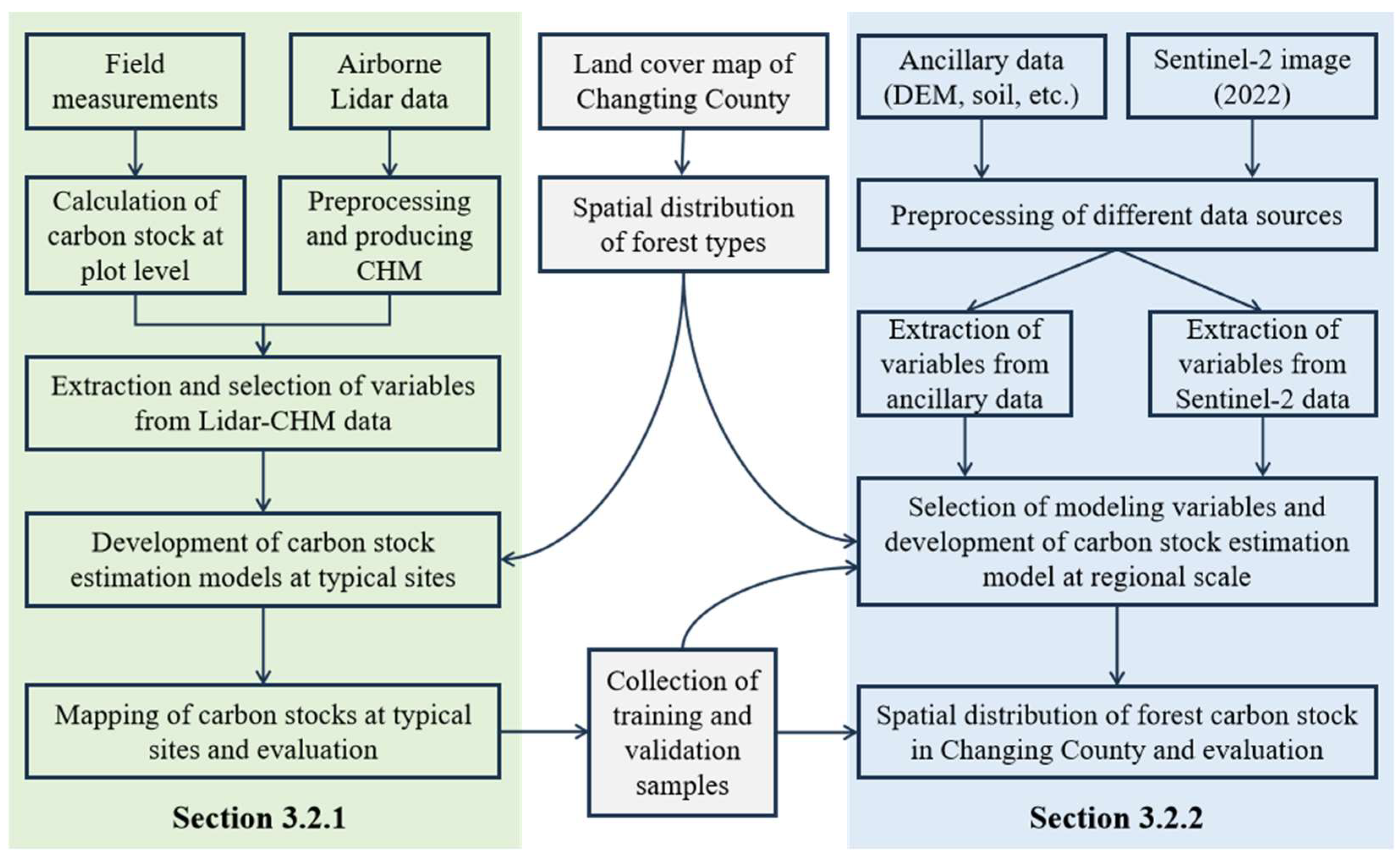
This study on forest carbon stock estimation consists of the following steps (see Figure 2): (1) data collection and preprocessing, including the calculation of carbon stock at the plot level based on field measurements, and preprocessing of the airborne Lidar, Sentinel-2, and ancillary data such as the digital elevation model (DEM); (2) the development of carbon stock estimation models at typical sites (airborne Lidar covered area) based on airborne Lidar-derived variables using linear regression and Bayesian hierarchical modeling methods; (3) the development of carbon stock estimation models at the regional scale based on Sentinel-2 and ancillary data by relating to forest carbon stock samples from typical sites; and (4) carbon stock mapping for Changting County using the developed model at the regional scale and a comparative analysis of the predicted carbon stocks between the conservation and non-conservation regions.

3.1. Datasets

The datasets used in this study included field measurements, airborne Lidar, Sentinel-2 multispectral images, land cover distribution, and ancillary data such as DEM, soil, and polygons related to conservation measures (see Table 1). Field measurements were conducted during the same timeframe as the airborne Lidar data acquisition in 2022, ensuring the reliability of forest carbon stock mapping in typical sites based on Lidar-derived variables. Although there are some differences among the data acquisition dates for the field surveys, airborne Lidar, and Sentinel-2 data, these date inconsistencies would not affect their use in this study, considering the very slow vegetation growth conditions in this region caused by long-term soil erosion. Here, we only used the Sentinel-2 L2A imagery on 23 October 2022 for carbon stock estimation at the regional scale. The Sentinel-2 data on 31 January 2021 were used in a previous study to develop the land use/cover map.

3.1.1. Field Measurements

Field measurements were conducted on similar dates as the airborne Lidar data acquisition dates, that is, field measurements in 7 typical sites in Changting County were conducted in January 2022, in the Luodihe watershed of Changting County and in Baisha State Forest Farm of Shanghang County in August 2022. A total of 84 sample plots, with each plot size being 20 m × 20 m (some plot sizes were 25.8 m × 25.8 m considering tree density), were collected, depending on the terrain conditions and tree density. Among those plots, 57 were located in Changting, including 43 Masson pine, 3 Chinese fir, and 11 broadleaf forests. Because of the limited number of sample plots of Chinese fir and broadleaf forests in Changting County, we used 21 Chinese fir and 6 broadleaf forests from Baisha State Forest Farm near Changting County. The coordinates of each plot were recorded using RTK for later co-registration with other datasets. Tree species within a plot were recorded, and the diameter at breast height (DBH) of individual trees was measured using a diameter tape. The carbon stock of each individual tree was calculated using an allometric equation specific to the tree species in Fujian Province (Table 2). The carbon stock of a plot was accumulated by adding up the carbon stocks of all individual trees, and then the carbon stock at plot size was converted to the carbon stock in tons per hectare (t/ha). The statistics of carbon stocks for all samples are summarized in Table 3, showing that Masson pine had the smallest mean values and Chinese fir had the largest mean values, because the Masson pine samples were mainly from the conservation regions in Changting County.

3.1.2. Airborne Lidar Data

Airborne Lidar data in 7 typical sites in Changting County were collected in January 2022 using the Zenmuse L1 Lidar system, and data for the Luodihe watershed in Changting County and Baisha State Forest Farm in Shanghang were collected in August 2022 using the RIEGL VUX-240 Lidar system. Both Lidar systems utilized near-infrared light with a pulse emission frequency of 1800 KHz, resulting in a point density of over 40 points/m2 on average, with a horizontal accuracy of 0.05 m and a vertical accuracy of 0.1 m. The Lidar point clouds were imported into Lidar360 software (version 7.2.4), and the noisy points including outliers and isolated points were removed. Additionally, the points corresponding to artificial objects such as towers and power lines were manually deleted from the Lidar point clouds. The remaining points were classified as ground points and canopy points. The ground points were used to generate a digital terrain model (DTM) with a cell size of 1 m × 1 m using the Improved Progressive TIN Densification (IPTD) method, while the canopy points were used to generate the same cell size of the digital surface model (DSM). The difference between the DSM and DTM was calculated to generate the canopy height model (CHM) data with a 1 m spatial resolution, representing the maximum canopy height within each pixel.

3.1.3. Sentinel-2 Multispectral Images

The Sentinel-2 L2A multispectral surface reflectance data, which were acquired on 23 October 2022, were obtained from the Google Earth Engine (GEE) website (https://earthengine.google.com, accessed on 7 September 2023). The data underwent orthorectification, geometric correction, and atmospheric correction, resulting in a new dataset with 10 spectral bands and a 10 m spatial resolution. Subsequently, topographic correction was performed using the SCS + C method based on the NASADEM data within the GEE platform [42].

3.1.4. Ancillary Data

Ancillary data used in this study included NASADEM, soil data, and land cover data (Table 1). The NASADEM dataset with a spatial resolution of 30 m was acquired from NASA Earth Data (https://lpdaac.usgs.gov/tools/earthdata-search/, accessed on 25 September 2023). According to the official release, the vertical accuracy of NASADEM was 5.3 m [43]. The product was not subjected to any further processing due to the lack of free and publicly available terrain data for calibration at the regional scale. The DEM played multiple roles in this study. Firstly, it was used in the topographic correction of Sentinel-2 images and for land cover classification as extra variables. Additionally, the DEM was utilized to generate the slope and aspect maps and facilitated the development of hydrological features such as flow direction, flow accumulation, and flow length, using the hydrology module in ArcGIS. These hydrological features were further employed in subsequent analyses.
The soil property data from OpenLandMap (https://openlandmap.org/, accessed on 25 September 2023) were acquired through Google Earth Engine (GEE). This dataset represents an enhanced version of the SoilGrids, offering predictions of various soil properties at a resolution of 250 m. These properties include the soil type, organic carbon (g/kg), bulk density (kg/cm3), pH level, soil texture class, soil available water content (%), soil clay content (kg/kg), and soil sand content (kg/kg) at six standard depths (0, 10, 30, 60, 100, and 200 cm). To align with other datasets, all soil layers were resampled to a cell size of 30 m × 30 m using the nearest neighbor method.
The land cover map of Changting County with a spatial resolution of 10 m was developed in our previous study [39]. This map was generated using the random forest method by combining Sentinel-2 images that were acquired on 31 January 2021 and DEM data. The land cover categories included Masson pine, Chinese fir, broadleaf forest, bamboo, and other non-forest types such as imperious surface area, water bodies, croplands, burned areas, and tea plantations. The overall accuracy of the land cover map was reported as 93.2%, with accuracies for all forest types exceeding 80%.
Because of the soil erosion problem in this study area, different conservation measures (i.e., restoring low-function forests, closing hillsides for afforestation, planting fruit trees, planting trees and grasses, constructing terraces on slope land, and multiple control measures) were adopted in the past three decades, as summarized in [39]. These measures with implementation dates were collected from the Soil Protection Station of Changting County and were organized into polygon vectors. Based on these polygon data, the county was grouped as conservation zones where different measures were implemented and non-conservation zones where no measures were implemented.

3.2. Methods

3.2.1. Forest Carbon Stock Mapping in Typical Sites Based on Lidar-Derived Variables

(1)
Extraction and selection of predictive variables from Lidar data
Canopy height metrics (such as the 10th, 20th, …, 90th, 95th height percentiles; maximum; minimum; mean; and median) and structure metrics such as the coefficient of variation (CV), skewness (SK), and kurtosis (KU) were calculated from the Lidar CHM at a window size of 20 m × 20 m, the same size as the sample plots. The values of these variables at sample plot locations, along with the carbon stock data, were extracted and exported into IBM SPSS software (version 20.0.0), where they were processed using descriptive statistics. Correlation coefficients between all variables and the carbon stock were computed. Due to the varying degrees of relationships between the carbon stock and predictive variables, as well as the high correlations among some predictive variables, it is necessary to eliminate unimportant variables to simplify the modeling. That is, variables with correlation values greater than 0.85 between each other were considered strongly correlated, and only the variables having stronger correlations with carbon stock were retained, while the others were removed. After this processing, a stepwise linear regression (SLR) was employed for the selection of modeling variables.
SLR determines the inclusion or exclusion of variables based on the significance of their estimated coefficients, assessed through a series of F-tests or T-tests [44]. It constructs a model iteratively, adding or removing variables one at a time. When a predictor is added or removed, the t-statistic of its estimated coefficient is calculated, and its significance is evaluated. The most significant variables are retained in the model, while the least significant ones are removed. This iterative process continues until the retained variables collectively yield the best estimates [45]. In this study, we used a significance level of 0.05 to decide whether a variable should be included or not. The variable selection processes were performed separately for stratification (different forest types) and non-stratification (one class as forest) scenarios. The selected variables were then used to develop carbon stock estimation models for the corresponding scenarios.
(2)
Construction of carbon stock estimation models based on the selected variables
Previous studies indicated that linear regression provided better modeling performance than machine learning algorithms when Lidar data were used for biomass or carbon stock estimation based on individual tree species or forest type [31,32]. In our previous studies, we found that the Bayesian hierarchical model (BHM) further improved the modeling performance and prediction accuracy. Therefore, two types of modeling methods—linear regression and BHM—were employed for carbon stock estimation modeling at typical sites.
With the advantages of simplicity and easy interpretation, linear regression was widely applied for biomass or carbon stock estimation modeling [3]. A previous study demonstrated that building models independently for each forest type (species) resulted in better estimation than a general model [31]. Therefore, we designed scenarios consisting of non-stratification and stratification. In the non-stratification scenario, the model was generated based on combined sample plots without differentiating forest types. In the stratification scenario, the model was developed based on the sample plots of specific forest types, namely, Masson pine, Chinese fir, and broadleaf forest in this study.
BHM is a statistical technique that involves structuring models at multiple levels, employing Bayesian methods to estimate the parameters of the posterior distribution [46]. This approach combines sub-models to create hierarchical models, integrating observational data using Bayesian theorem to account for uncertainty. It allows for the simultaneous modeling of different data levels, effectively capturing dependencies and nesting within the data [47].
Two factors, i.e., forest type (pine, Chinese fir, and broadleaf) and environmental conditions such as soil subgroups (Argi-Udic Ferrosols and Ali-Udic Cambosols), conservation and non-conservation zones, and slope groups, were used in the BHM. Different forest types (or tree species) have their own relationships between tree height and carbon stock; thus, forest type is a common factor for use as a stratification factor [31]. Considering the special characteristics of this study area, that is, the soil erosion problem, the major factors that affected soil erosion severity were used in the BHM. Topographic factors such as the slope and soil types were two important factors resulting in different levels of soil erosion severity, thus causing different growth conditions [48,49], while conservation measures reduced the soil erosion problem and thus improved forest growth [39]. Therefore, these factors were used as stratification factors in the BHM approach. The predictive variables used in the BHM consisted of two parts: fixed effect variables and random effect variables. SLR was conducted on all samples and grouped samples to select these two types of variables, as reported in previous studies [32].
The modeling results were evaluated with the leave-one-out cross-validation (LOOCV) method in this study, considering the limited number of sample plots for each forest type. LOOCV involves training the model n times, where n is the number of observations, using each observation once as a test set while the remaining n − 1 observations serve as the training set. Common parameters such as the coefficient of determination (R2), root mean square error (RMSE), and relative root mean square error (RMSE%) were used [32]. Through comparison of the modeling performances, the best one was selected for the prediction of the forest carbon stock distribution for the typical sites, which was used for providing sample plots for regional forest carbon stock estimation modeling.

3.2.2. Forest Carbon Stock Mapping at Regional Scale Using Sentinel-2 and Ancillary Data

The samples for developing regional forest carbon stock estimation models were extracted from the predicted values at typical sites using airborne Lidar data, taking the different forest types and age groups into account. Based on the distribution of Masson pine, Chinese fir, and broadleaf forest in these typical sites, 400 samples, including 200 for Masson pine and 100 each for Chinese fir and broadleaf forest, were collected. A total of 60% of the samples were used for modeling and the rest for validation.
The variables extracted from Sentinel-2 and the ancillary data are summarized in Table 4. At the pixel level, in addition to the spectral bands, different vegetation indices such as the normalized difference vegetation index (NDVI) and soil adjusted vegetation index (SAVI) were calculated. At the spatial level, the gray-level co-occurrence matrix (GLCM) textural measures were used to calculate textural images using a window size of 9 × 9 pixels based on individual spectral bands. We also extracted variables from the ancillary data such as the DEM and soil. The slope and slope aspect were directly calculated from the DEM data, while the hydrological variables such as the flow direction, flow accumulation, and flow length that are directly related to soil erosion were also calculated from the DEM data using the hydrology module in the ArcGIS software (version 10.6). The soil-related variables such as the soil type, organic carbon, bulk density, pH level, soil texture class, soil available water content, soil clay content, and soil sand content at six standard depths (0, 10, 30, 60, 100, and 200 cm) were extracted from the downloaded soil data.
Previous research indicated that random forest was an important tool for developing forest carbon stock estimation models, especially when the modeling variables were from different data sources [50,51]. The random forest algorithm is an ensemble of the decision tree algorithm through the averaging of the results from different decision trees [52]. One important advantage of using random forest is that it can reduce the overfitting problem that is common in machine learning algorithms. Another important feature is its insensitivity to noises; thus, it can use different kinds of variables for modeling. Therefore, random forest is extensively used in different applications such as forest classification [53] and carbon stock estimation [30,50].
One valuable feature when using random forest is the importance ranking, which is used to select key modeling variables. All variables from different data sources as listed in Table 4 were used as input in random forest, where the carbon stock of samples was used as the dependent variable. In the random forest algorithm, the number of decision trees (ntree), the number of variables for each split (mtry), and the minimum leaf size (nleaf) are three parameters that need to be optimized. The mtry parameter controls the number of randomly selected features when each node splits. By default, the value of mtry is one-third of the number of input variables [29]. In this study, the ntree value was 2000, the mtry value was 3, and the nleaf, based on the default in randomForest in R, was set to 5. The optimized random forest model was used to predict the forest carbon stock for the entire study area, and the results were evaluated using the validation samples. The R2, RMSE, and RMSE% were used to evaluate the regional forest carbon stock estimation results.

4. Results

4.1. Analysis of Forest Carbon Stock Estimation Results in Typical Sites

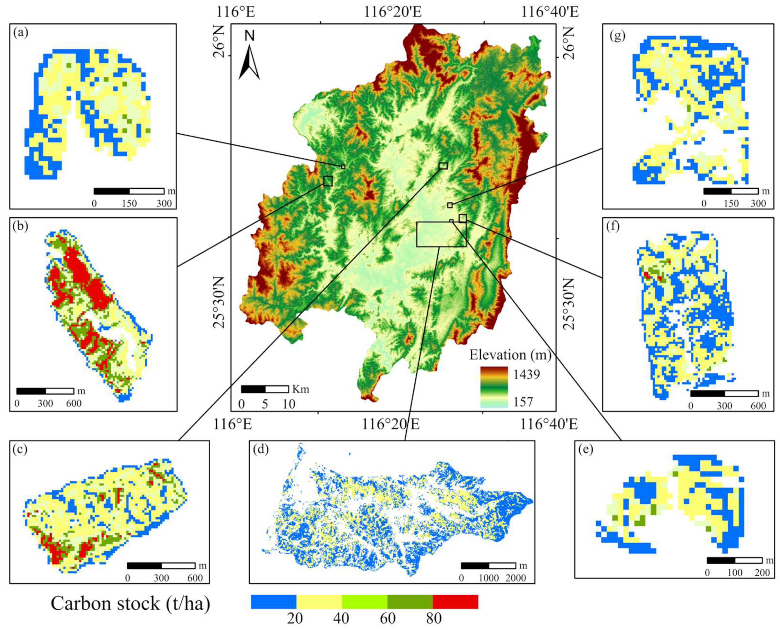
The modeling results using linear regression (Table 5) indicated that the modeling strategy was better for individual tree species—Masson pine and Chinese fir had much better performance than the non-stratification modeling strategy, implying the importance of developing a carbon stock estimation model for a specific forest type. Table 5 also shows that the BHM provided better modeling performance than linear regression. However, the use of either soil type, erosion control, or slope group as a stratification factor in the BHM had similar modeling performances (Figure 3), implying that, in addition to forest type, the use of one factor that was strongly related to the soil erosion condition was needed in the BHM modeling. The best model was used to predict the forest carbon distribution at the typical sites (Figure 4), indicating that some regions (e.g., a, b, c) had carbon stock of 20–80 t/ha, and some regions due to severe soil erosion problem (e.g., d, e, f, g) had carbon stock of less than 40 t/ha.

4.2. Analysis of Forest Carbon Stock Estimation Results at Regional Scale

The selected variables for modeling the forest carbon stock estimation included pixel-based bands (nitrogen reflectance index—NRI), textural images (second moment and contrast based on red band, and correlation based on blue band), and ancillary data (soil-based variables such as the soil bulk density, soil organic carbon, pH level, and soil available water content; DEM-derived elevation and slope), indicating the important roles of different data sources in developing a regional forest carbon stock estimation model. The selected vegetation index and textural images show that it is necessary to use optical sensor data that effectively represent the different forest canopy features, and the selected variables from the soil and DEM data indicate the need to incorporate the environmental conditions that affect vegetation growth to enhance modeling performance.
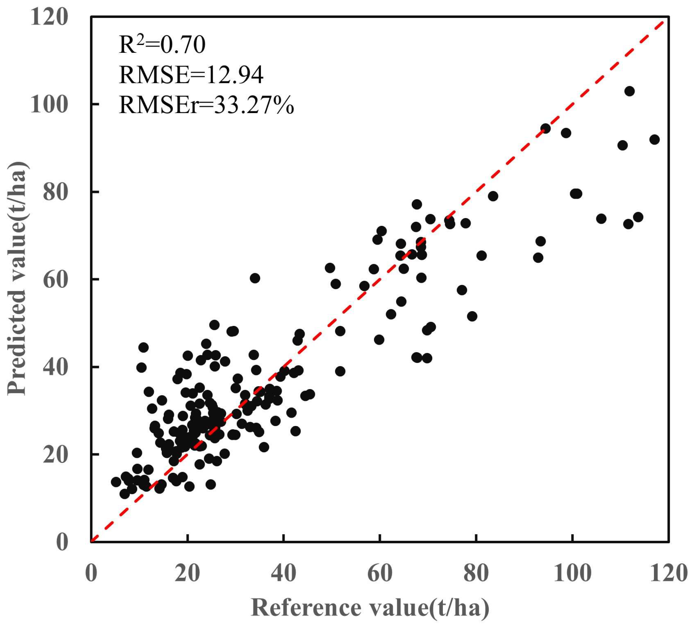
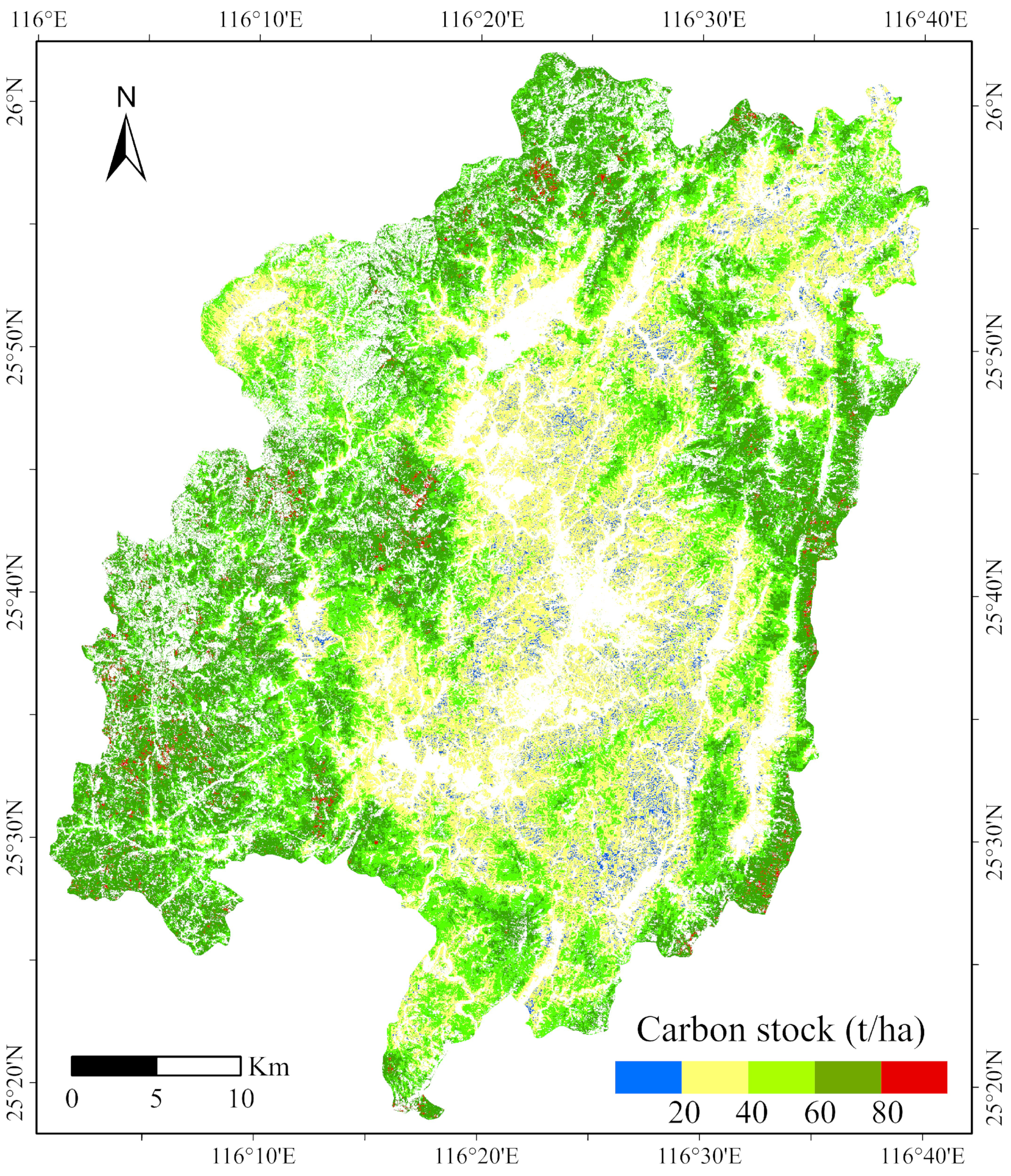
The evaluation of the prediction results (Figure 5) showed a good modeling performance with an R2 of 0.7 and RMSE of 12.94 t/ha. The figure shows the common problem that overestimation existed when the carbon stock was relatively small such as less than 20 t/ha, and underestimation existed when the carbon stock was larger than 80 t/ha, which is the same conclusion as in previous publications when the random forest method was used to develop biomass or carbon stock estimation models because of the overfitting problem and data saturation problem [18,31]. Based on the statistical analysis of the predicted carbon stock in Changting County (Figure 6), a carbon stock value of less than 20 t/ha accounted for 3.78% and a value of greater than 80 t/ha accounted for only 0.86%; most regions had carbon stock values within the range between 20 t/ha and 80 t/ha. Figure 6 indicates the different spatial patterns of the carbon stock distribution in the county, that is, the western and eastern parts had higher values (greater than 60 t/ha) than the central and southern parts (less than 40 t/ha). The carbon stock was especially low in Hetian basin due to a serious soil erosion problem in the past decades.

4.3. Comparison of Carbon Stock between Conservation and Non-Conservation Regions

Based on the statistical results from the predicted carbon stock in this study area, we found that overall, Chinese fir and broadleaf forests had higher carbon stock (12.1–13.6 t/ha higher) than Masson pine, and non-conservation regions had 15.2–16.1 t/ha higher carbon stock than conservation regions had (Table 6). A comparison of the spatial distributions between the predicted carbon stock (Figure 6) and classified forest types (Figure 1b) indicated that Masson pine forests were mainly distributed in the conservation regions, where other forest types such as Chinese fir could not grow well because of the poor soil conditions. In the conservation regions, the bare lands with poor soil conditions in the initial stage made the growth of trees or grasses difficult. The Masson pine with its tolerance of poor soil conditions can grow slowly. Therefore, Masson pine forests had much smaller carbon stocks than the other forest types.

5. Discussion

5.1. The Role of Airborne Lidar Data in Regional Carbon Stock Estimation

The collection of samples from field measurements is the most accurate method but is a challenging task due to labor intensity and cost. So far, there are no quantitative criteria for the required number of samples for modeling, depending on the specific study area. In general, at least 30 samples are needed according to statistical theory, but many previous studies did not have this number for modeling, especially in tropical regions where field measurements were very difficult [54,55]. In reality, a small number of samples often results in poor modeling performance and prediction accuracy because the developed model lacks robustness and representativeness [3,56]. One solution is to estimate the carbon stock from a high density of point cloud data [15]. As airborne Lidar data are easily available, the Lidar-derived estimation results become an alternative for providing a large number of samples for modeling and validation in a large area [15,19,20]. The key is to produce an accurate estimation from airborne Lidar data. This study explored the combination of limited field measurements from different sites and Lidar-derived variables to develop a carbon stock estimation model using the BHM (R2 = 0.91, RMSE = 7.25 t/ha) and found that it was a feasible method to produce good representative samples at spatial scale (for example, the maximum carbon stock changed from 103.99 t/ha in the survey data to 119 t/ha in the Lidar-based prediction), providing a new way for regional carbon stock estimation modeling. Unfortunately, this study lacked sufficient samples (e.g., 17 samples for broadleaf forest) to directly establish the robust relationship between field samples and multi-source data (e.g., Sentinel-2 and auxiliary data). Because this relationship is not a simple linear relationship, machine learning algorithms are often used but need a large number of samples for training. It is still unclear how much error may be generated from the continuous procedure: from sample plots to Lidar-based estimation and then to Sentinel-2 based estimation. However, Jiang et al. [25] found that errors accumulated from the Lidar-based models to the RF models did not simply add up and might cancel each other out, thus improving the estimation performance. More research is needed to examine different uncertainty levels from multi-stages—field measurements at the plot level, Lidar-based modeling at typical sites, and Sentinel-2 based modeling at the regional scale—to improve the understanding of error accumulation.

5.2. The Need to Develop Proper Modeling Methods for Different Sites

Linear regression was proven effective for developing carbon stock estimation models when Lidar data were used for a specific forest type [57]. However, if the number of samples is not big enough to develop a robust estimation model or the samples are from different study areas, the linear regression approach may not be a proper choice [58]. In this situation, the BHM can solve this problem because it can not only effectively use the general rules from the samples of different sites but can also use the specific characteristics of different sites through the use of the hierarchical-based modeling method [32]. An advantage of using the BHM over linear regression is that it makes it possible to develop more accurate modeling results with limited samples from different sites, as proven in this study. Because the forest stand structures of different forest types are influenced by terrain, soil, and climate conditions in a large area [58,59], the ability to use the BHM with multiple stratification factors by incorporating these conditions can provide better modeling performance than non-stratification modeling. This study confirmed that incorporating environmental factors (e.g., soil type, terrain slope) and human factors (e.g., conservation measures) as stratification variables in the BHM significantly enhanced its accuracy compared to a BHM without stratification. In reality, which environmental factors should be used in the BHM depends on the characteristics of the study area under investigation. The adaptability of this approach highlights its prospects for broad application, suggesting that future research could explore its utility in diverse ecological contexts.

5.3. The Need to Use Multi-Source Data for Developing Forest Carbon Stock Estimation Model

Previous studies indicated that forest biomass or carbon stock estimation using optical sensor data had obvious overestimation and underestimation problems [29], and this study also had the same problem. However, this study had better modeling performance and better prediction accuracy than previous studies such as those conducted in the subtropical regions of Zhejiang Province (e.g., [18,29]). The major reason was the relatively poor soil fertility in this region due to the soil erosion problem resulting in relatively simple stand structures and less dense canopies; thus, data saturation was not a serious problem. For example, the biomass saturation value for Masson pine was 159 t/ha, for Chinese fir 143 t/ha, and for broadleaf forest 123 t/ha in the subtropical region of Zhejiang Province [18]. Considering the carbon coefficients of 0.4597, 0.499, and 0.4901 for Masson pine, Chinese fir, and broadleaf forest, the saturation values were 73.1, 71.4, and 60.3 t/ha, respectively, and these values were much higher than they were in Changting County with average carbon values of 43.44, 55.51, and 57.04 t/ha, implying that the impact of the saturation problem on modeling performance was much less in this study area than in other regions.
Because Lidar data are not always available, especially in a large area considering the cost for data collection and the huge data volume, optical sensor data such as Landsat and Sentinel-2 data at no cost are still the most important data sources for regional carbon stock estimation [60,61]. As many previous studies indicated that pure optical sensor data did not provide satisfactory modeling results, especially for forest sites with high carbon stocks resulting in signal saturation, it is necessary to make full use of the advantages of different data sources. The complexity of the forest stand structure and the tree species composition are related to topography, soil, and climate [59]. The critical step is to identify key variables for developing estimation models for a specific forest type because of the different impacts of the environmental conditions on the individual forest growth [31]. As shown in this study, where the selected variables were from Sentinel-2, DEM, and soil data, by using the importance ranking function in random forest, more research is still needed to effectively identify the key variables from different data sources; meanwhile, it is important to reduce the effects of different data quality levels and the spatial resolutions of multiple data sources on the modeling performance.

6. Conclusions

This study explored a method for mapping the forest carbon stock distribution at the regional scale through the combined use of a limited number of sample plots, airborne Lidar, Sentinel-2 multispectral bands, and ancillary data. A comparative analysis of linear regression and BHM for carbon stock estimation at typical sites indicated that the dual factors of forest type and soil erosion control provided the best modeling performance with an R2 value of 0.91, RMSE of 7.25 t/ha, and RMSE% of 21.55%. The good modeling performance at typical sites provided the chance to select sufficient modeling and validation samples for regional carbon stock estimation modeling. The modeling results based on Sentinel-2 and ancillary data at the regional scale showed the feasibility of the method to develop forest carbon stock estimation models with an R2 value of 0.70, RMSE of 12.94 t/ha, and RMSE% of 33.27%. The spatial distribution of the forest carbon stock estimation provided the necessary data source for implementing proper measures and making decisions to reduce the soil erosion problem. The results showed that the conservation regions had lower carbon stock values than the non-conservation regions, with about 15 t/ha lower values for different forest types. Masson pine is a critical tree species that can grow in regions with a serious soil erosion problem, but the average carbon stock is much smaller than other regions without serious soil erosion. This study provides an effective method to estimate the forest carbon stock in a large area, which provides important data sources for evaluating the effects of implementing conservation measures in improving the degraded forest ecosystem functions through comparative analysis of the carbon stock among different regions. The strategy of using the combination of field measurements, airborne Lidar, Sentinel-2 multispectral bands, and ancillary data provides new insights for accurately mapping the carbon stock distribution at the regional scale for degraded forest ecosystems.

Author Contributions

Conceptualization, D.L. (Dengsheng Lu) and Q.W.; methodology, D.L. (Dengsheng Lu), G.L., D.L. (Dengqiu Li), Q.W., J.R. and X.S.; software, D.L. (Dengsheng Lu) and X.S.; validation, Q.W., J.R. and X.S.; formal analysis, G.L. and X.S.; investigation, D.L. (Dengqiu Li), Q.W., J.R. and X.S.; resources, D.L. (Dengsheng Lu), G.L., D.L. (Dengqiu Li) and Q.W.; data curation, D.L. (Dengqiu Li), Q.W., J.R. and X.S.; writing—original draft preparation, X.S., G.L. and D.L. (Dengsheng Lu).; writing—review and editing, D.L. (Dengsheng Lu), G.L., D.L. (Dengqiu Li), Q.W. and X.S.; visualization, D.L. (Dengsheng Lu), G.L. and D.L. (Dengqiu Li).; supervision, D.L. (Dengsheng Lu) and G.L.; project administration, D.L. (Dengsheng Lu) and D.L. (Dengqiu Li); funding acquisition, D.L. (Dengsheng Lu) and D.L. (Dengqiu Li). All authors have read and agreed to the published version of the manuscript.

Funding

This study was supported by the National Key R&D Program of China (grant No. 2021YFD2200400102), Fujian Provincial Science and Technology Department (grant No. 2021R1002008), Department of Water Resources at Fujian Province (grant No. MSK202207 and MSK202311), and Ministry of Water Resources (grant No. SKS-2022083).

Data Availability Statement

Data sources such as field survey can be obtained from Dengsheng Lu at Fujian Normal University upon request.

Acknowledgments

The authors would like to thank Wenlin Yang, Yongpeng Ye, Ming Zhang, Xu Zhang, Aoni Shi, and Ganlin Feng for their help during the field survey.

Conflicts of Interest

The authors declare no conflicts of interest. The funders had no role in the design of the study; in the collection, analyses, or interpretation of data; in the writing of the manuscript; or in the decision to publish the results.

References

  1. Cook-Patton, S.C.; Leavitt, S.M.; Gibbs, D.; Harris, N.L.; Lister, K.; Anderson-Teixeira, K.J.; Briggs, R.D.; Chazdon, R.L.; Crowther, T.W.; Ellis, P.W.; et al. Mapping Carbon Accumulation Potential from Global Natural Forest Regrowth. Nature 2020, 585, 545–550. [Google Scholar] [CrossRef]
  2. Soto-Navarro, C.; Ravilious, C.; Arnell, A.; de Lamo, X.; Harfoot, M.; Hill, S.; Wearn, O.; Santoro, M.; Bouvet, A.; Mermoz, S.; et al. Mapping Co-Benefits for Carbon Storage and Biodiversity to Inform Conservation Policy and Action. Philos. Trans. R. Soc. B Biol. Sci. 2020, 375, 20190128. [Google Scholar] [CrossRef]
  3. Lu, D.; Chen, Q.; Wang, G.; Liu, L.; Li, G.; Moran, E. A Survey of Remote Sensing-Based Aboveground Biomass Estimation Methods in Forest Ecosystems. Int. J. Digit. Earth 2016, 9, 63–105. [Google Scholar] [CrossRef]
  4. Sun, W.; Liu, X. Review on Carbon Storage Estimation of Forest Ecosystem and Applications in China. For. Ecosyst. 2019, 7, 4. [Google Scholar] [CrossRef]
  5. Qin, S.; Nie, S.; Guan, Y.; Zhang, D.; Wang, C.; Zhang, X. Forest Emissions Reduction Assessment Using Airborne LiDAR for Biomass Estimation. Resour. Conserv. Recycl. 2022, 181, 106224. [Google Scholar] [CrossRef]
  6. Cook-Patton, S.C.; Shoch, D.; Ellis, P.W. Dynamic Global Monitoring Needed to Use Restoration of Forest Cover as a Climate Solution. Nat. Clim. Change 2021, 11, 366–368. [Google Scholar] [CrossRef]
  7. Araza, A.; de Bruin, S.; Herold, M.; Quegan, S.; Labriere, N.; Rodriguez-Veiga, P.; Avitabile, V.; Santoro, M.; Mitchard, E.T.A.; Ryan, C.M.; et al. A Comprehensive Framework for Assessing the Accuracy and Uncertainty of Global above-Ground Biomass Maps. Remote Sens. Environ. 2022, 272, 112917. [Google Scholar] [CrossRef]
  8. Xiao, J.; Chevallier, F.; Gomez, C.; Guanter, L.; Hicke, J.A.; Huete, A.R.; Ichii, K.; Ni, W.; Pang, Y.; Rahman, A.F.; et al. Remote Sensing of the Terrestrial Carbon Cycle: A Review of Advances over 50 Years. Remote Sens. Environ. 2019, 233, 111383. [Google Scholar] [CrossRef]
  9. Zhao, J.; Liu, D.; Cao, Y.; Zhang, L.; Peng, H.; Wang, K.; Xie, H.; Wang, C. An Integrated Remote Sensing and Model Approach for Assessing Forest Carbon Fluxes in China. Sci. Total Environ. 2022, 811, 152480. [Google Scholar] [CrossRef]
  10. Grant, R.F.; Oechel, W.C.; Ping, C.L. Modelling Carbon Balances of Coastal Arctic Tundra under Changing Climate. Glob. Change Biol. 2003, 9, 16–36. [Google Scholar] [CrossRef]
  11. Zhou, W.; Guan, K.; Peng, B.; Tang, J.; Jin, Z.; Jiang, C.; Robert, G.; Mezbahuddin, S. Quantifying carbon budget, crop yields and their responses to environmental variability using the ecosys model for US Midwestern agroecosystems. Agric. For. Meteorol. 2021, 307, 108521. [Google Scholar] [CrossRef]
  12. Nguyen, T.; Jones, S.; Soto-Berelov, M.; Haywood, A.; Hislop, S. Landsat Time-Series for Estimating Forest Aboveground Biomass and Its Dynamics across Space and Time: A Review. Remote Sens. 2019, 12, 98. [Google Scholar] [CrossRef]
  13. Emick, E.; Babcock, C.; White, G.W.; Hudak, A.T.; Domke, G.M.; Finley, A.O. An Approach to Estimating Forest Biomass While Quantifying Estimate Uncertainty and Correcting Bias in Machine Learning Maps. Remote Sens. Environ. 2023, 295, 113678. [Google Scholar] [CrossRef]
  14. Ma, T.; Zhang, C.; Ji, L.; Zuo, Z.; Beckline, M.; Hu, Y.; Li, X.; Xiao, X. Development of Forest Aboveground Biomass Estimation, Its Problems and Future Solutions: A Review. Ecol. Indic. 2024, 159, 111653. [Google Scholar] [CrossRef]
  15. Lu, D.; Jiang, X. A Brief Overview and Perspective of Using Airborne Lidar Data for Forest Biomass Estimation. Int. J. Image Data Fusion 2024, 15, 1–24. [Google Scholar] [CrossRef]
  16. Lu, D.; Chen, Q.; Wang, G.; Moran, E.; Batistella, M.; Zhang, M.; Vaglio Laurin, G.; Saah, D. Aboveground Forest Biomass Estimation with Landsat and LiDAR Data and Uncertainty Analysis of the Estimates. Int. J. For. Res. 2012, 2012, 436537. [Google Scholar] [CrossRef]
  17. Hu, Y.; Sun, Z. Assessing the Capacities of Different Remote Sensors in Estimating Forest Stock Volume Based on High Precision Sample Plot Positioning and Random Forest Method. Nat. Environ. Pollut. Technol. 2022, 21, 1113–1123. [Google Scholar] [CrossRef]
  18. Zhao, P.; Lu, D.; Wang, G.; Wu, C.; Huang, Y.; Yu, S. Examining Spectral Reflectance Saturation in Landsat Imagery and Corresponding Solutions to Improve Forest Aboveground Biomass Estimation. Remote Sens. 2016, 8, 469. [Google Scholar] [CrossRef]
  19. Coops, N.C.; Tompalski, P.; Goodbody, T.R.H.; Queinnec, M.; Luther, J.E.; Bolton, D.K.; White, J.C.; Wulder, M.A.; van Lier, O.R.; Hermosilla, T. Modelling Lidar-Derived Estimates of Forest Attributes over Space and Time: A Review of Approaches and Future Trends. Remote Sens. Environ. 2021, 260, 112477. [Google Scholar] [CrossRef]
  20. Puliti, S.; Breidenbach, J.; Schumacher, J.; Hauglin, M.; Klingenberg, T.F.; Astrup, R. Above-Ground Biomass Change Estimation Using National Forest Inventory Data with Sentinel-2 and Landsat. Remote Sens. Environ. 2021, 265, 112644. [Google Scholar] [CrossRef]
  21. Silveira, E.M.O.; Radeloff, V.C.; Martinuzzi, S.; Martinez Pastur, G.J.; Bono, J.; Politi, N.; Lizarraga, L.; Rivera, L.O.; Ciuffoli, L.; Rosas, Y.M.; et al. Nationwide Native Forest Structure Maps for Argentina Based on Forest Inventory Data, SAR Sentinel-1 and Vegetation Metrics from Sentinel-2 Imagery. Remote Sens. Environ. 2023, 285, 113391. [Google Scholar] [CrossRef]
  22. Ni, W.; Yu, T.; Pang, Y.; Zhang, Z.; He, Y.; Li, Z.; Sun, G. Seasonal Effects on Aboveground Biomass Estimation in Mountainous Deciduous Forests Using ZY-3 Stereoscopic Imagery. Remote Sens. Environ. 2023, 289, 113520. [Google Scholar] [CrossRef]
  23. Shen, W.; Li, M.; Huang, C.; Tao, X.; Wei, A. Annual Forest Aboveground Biomass Changes Mapped Using ICESat/GLAS Measurements, Historical Inventory Data, and Time-Series Optical and Radar Imagery for Guangdong Province, China. Agric. For. Meteorol. 2018, 259, 23–38. [Google Scholar] [CrossRef]
  24. Dalponte, M.; Jucker, T.; Liu, S.; Frizzera, L.; Gianelle, D. Characterizing Forest Carbon Dynamics Using Multi-Temporal Lidar Data. Remote Sens. Environ. 2019, 224, 412–420. [Google Scholar] [CrossRef]
  25. Jiang, X.; Li, D.; Li, G.; Lu, D. Eucalyptus Carbon Stock Estimation in Subtropical Regions with the Modeling Strategy of Sample Plots–Airborne LiDAR–Landsat Time Series Data. For. Ecosyst. 2023, 10, 100149. [Google Scholar] [CrossRef]
  26. Dong, P.; Chen, Q. LiDAR Remote Sensing and Applications; CRC Press, Taylor & Francis Group: New York, NY, USA, 2017. [Google Scholar]
  27. Poorazimy, M.; Shataee, S.; McRoberts, R.E.; Mohammadi, J. Integrating Airborne Laser Scanning Data, Space-Borne Radar Data and Digital Aerial Imagery to Estimate Aboveground Carbon Stock in Hyrcanian Forests, Iran. Remote Sens. Environ. 2020, 240, 111669. [Google Scholar] [CrossRef]
  28. Oehmcke, S.; Li, L.; Trepekli, K.; Revenga, J.C.; Nord-Larsen, T.; Gieseke, F.; Igel, C. Deep Point Cloud Regression for above-Ground Forest Biomass Estimation from Airborne LiDAR. Remote Sens. Environ. 2024, 302, 113968. [Google Scholar] [CrossRef]
  29. Gao, Y.; Lu, D.; Li, G.; Wang, G.; Chen, Q.; Liu, L.; Li, D. Comparative Analysis of Modeling Algorithms for Forest Aboveground Biomass Estimation in a Subtropical Region. Remote Sens. 2018, 10, 627. [Google Scholar] [CrossRef]
  30. Xie, D.; Huang, H.; Feng, L.; Sharma, R.P.; Chen, Q.; Liu, Q.; Fu, L. Aboveground Biomass Prediction of Arid Shrub-Dominated Community Based on Airborne LiDAR through Parametric and Nonparametric Methods. Remote Sens. 2023, 15, 3344. [Google Scholar] [CrossRef]
  31. Jiang, X.; Li, G.; Lu, D.; Erxue, C.; Wei, X. Stratification-Based Forest Aboveground Biomass Estimation in a Subtropical Region Using Airborne Lidar Data. Remote Sens. 2020, 12, 1101. [Google Scholar] [CrossRef]
  32. Lin, W.; Lu, Y.; Li, G.; Jiang, X.; Lu, D. A Comparative Analysis of Modeling Approaches and Canopy Height-Based Data Sources for Mapping Forest Growing Stock Volume in a Northern Subtropical Ecosystem of China. GISci. Remote Sens. 2022, 59, 568–589. [Google Scholar] [CrossRef]
  33. Bouvier, M.; Durrieu, S.; Fournier, R.A.; Saint-Geours, N.; Guyon, D.; Grau, E.; de Boissieu, F. Influence of Sampling Design Parameters on Biomass Predictions Derived from Airborne LiDAR Data. Can. J. Remote Sens. 2019, 45, 650–672. [Google Scholar] [CrossRef]
  34. Nuthammachot, N.; Askar, A.; Stratoulias, D.; Wicaksono, P. Combined Use of Sentinel-1 and Sentinel-2 Data for Improving above-Ground Biomass Estimation. Geocarto Int. 2022, 37, 366–376. [Google Scholar] [CrossRef]
  35. Chen, Z. Desertification Induced by Water Erosion and Its Combat of Hetian Town in Changding County, Fujian Province. Prog. Geogr. 1998, 17, 67–72. [Google Scholar]
  36. Zeng, J.; Zhong, B. Historical Changes in Strategies to Control Soil and Water Erosion in Changting County. Subtrop. Soil Water Conserv. 2002, 14, 37–39. [Google Scholar]
  37. Wang, C.; Yang, Y.; Zhang, Y. Rural Household Livelihood Change, Fuelwood Substitution, and Hilly Ecosystem Restoration: Evidence from China. Renew. Sustain. Energy Rev. 2012, 16, 2475–2482. [Google Scholar] [CrossRef]
  38. Gao, J.; Shi, C.; Yang, J.; Yue, H.; Liu, Y.; Chen, B. Analysis of Spatiotemporal Heterogeneity and Influencing Factors of Soil Erosion in a Typical Erosion Zone of the Southern Red Soil Region, China. Ecol. Indic. 2023, 154, 110590. [Google Scholar] [CrossRef]
  39. Sun, X.; Li, G.; Wu, Q.; Li, D.; Lu, D. Examining the Effects of Soil and Water Conservation Measures on Patterns and Magnitudes of Vegetation Cover Change in a Subtropical Region Using Time Series Landsat Imagery. Remote Sens. 2024, 16, 714. [Google Scholar] [CrossRef]
  40. LY/T 2263-2014; Tree Biomass Models and Related Parameters to Carbon Accounting for Pinus massoniana. Standards Press of China: Beijing, China, 2014.
  41. LY/T 2264-2014; Tree Biomass Models and Related Parameters to Carbon Accounting for Cunninghamia lanceolata. Standards Press of China: Beijing, China, 2014.
  42. Poortinga, A.; Tenneson, K.; Shapiro, A.; Nguyen, Q.; San Aung, K.; Chishtie, F.; Saah, D. Mapping Plantations in Myanmar by Fusing Landsat-8, Sentinel-2 and Sentinel-1 Data along with Systematic Error Quantification. Remote Sens. 2019, 11, 831. [Google Scholar] [CrossRef]
  43. Buckley, S.M.; Agram, P.S.; Belz, J.E.; Crippen, R.E.; Gurrola, E.M.; Hensley, S.; Kobrick, M.; Lavalle, M.; Martin, J.M.; Neumann, M.; et al. NASADEM: User Guide (Technical Report January). 2020. Available online: https://lpdaac.usgs.gov/documents/592/NASADEM_User_Guide_V1.pdf (accessed on 8 June 2021).
  44. Draper, N.R.; Smith, H. Applied Regression Analysis; John Wiley & Sons, Inc.: Hoboken, NJ, USA, 1998. [Google Scholar]
  45. Tan, L.; Liu, H.; Tan, L. Algorithm Comparative Analysis with Stepwise Linear Regression and Neural Network. J. North China Univ. Sci. Technol. 2014, 11, 6. [Google Scholar]
  46. Arhonditsis, G.B.; Stow, C.A.; Steinberg, L.J.; Kenney, M.A.; Lathrop, R.C.; McBride, S.J.; Reckhow, K.H. Exploring Ecological Patterns with Structural Equation Modeling and Bayesian Analysis. Ecol. Model. 2006, 192, 385–409. [Google Scholar] [CrossRef]
  47. Bürkner, P.C. Brms: An R Package for Bayesian Multilevel Models Using Stan. J. Stat. Softw. 2017, 80, 1–28. [Google Scholar] [CrossRef]
  48. Huang, J.; Lu, D.; Li, J.; Wu, J.; Chen, S.; Zhao, W.; Ge, H.; Huang, X.; Yan, X.-D. Integration of Remote Sensing and GIS for Evaluating Soil Erosion Risk in Northwestern Zhejiang, China. Photogramm. Eng. Remote Sens. 2012, 78, 935–946. [Google Scholar] [CrossRef]
  49. Cheng, Z.; Lu, D.; Li, G.; Huang, J.; Sinha, N.; Zhi, J.; Li, S. A Random Forest-Based Approach to Map Soil Erosion Risk Distribution in Hickory Plantations in Western Zhejiang Province, China. Remote Sens. 2018, 10, 1899. [Google Scholar] [CrossRef]
  50. Marchesan, J.; Alba, E.; Schuh, M.S.; Favarin, J.A.S.; Fantinel, R.A.; Marchesan, L.; Pereira, R.S. Aboveground Biomass Stock and Change Estimation in Amazon Rainforest Using Airborne Light Detection and Ranging, Multispectral Data, and Machine Learning Algorithms. J. Appl. Remote Sens. 2023, 17, 24509. [Google Scholar] [CrossRef]
  51. Gao, L.; Chai, G.; Zhang, X. Above-Ground Biomass Estimation of Plantation with Different Tree Species Using Airborne LiDAR and Hyperspectral Data. Remote Sens. 2022, 14, 2568. [Google Scholar] [CrossRef]
  52. Belgiu, M.; Drǎguţ, L. Random Forest in Remote Sensing: A Review of Applications and Future Directions. ISPRS J. Photogramm. Remote Sens. 2016, 114, 24–31. [Google Scholar] [CrossRef]
  53. Yu, X.; Lu, D.; Jiang, X.; Li, G.; Chen, Y.; Li, D.; Chen, E. Examining the Roles of Spectral, Spatial, and Topographic Features in Improving Land-Cover and Forest Classifications in a Subtropical Region. Remote Sens. 2020, 12, 2907. [Google Scholar] [CrossRef]
  54. Lu, D.; Batistella, M.; Moran, E. Satellite Estimation of Aboveground Biomass and Impacts of Forest Stand Structure. Photogramm. Eng. Remote Sens. 2005, 71, 967–974. [Google Scholar] [CrossRef]
  55. Feng, Y.; Lu, D.; Chen, Q.; Keller, M.; Moran, E.; dos-Santos, M.N.; Bolfe, E.L.; Batistella, M. Examining Effective Use of Data Sources and Modeling Algorithms for Improving Biomass Estimation in a Moist Tropical Forest of the Brazilian Amazon. Int. J. Digit. Earth 2017, 10, 996–1016. [Google Scholar] [CrossRef]
  56. Ploton, P.; Mortier, F.; Réjou-Méchain, M.; Barbier, N.; Picard, N.; Rossi, V.; Dormann, C.; Cornu, G.; Viennois, G.; Bayol, N.; et al. Spatial Validation Reveals Poor Predictive Performance of Large-Scale Ecological Mapping Models. Nat. Commun. 2020, 11, 4540. [Google Scholar] [CrossRef] [PubMed]
  57. Nie, S.; Wang, C.; Zeng, H.; Xi, X.; Li, G. Above-Ground Biomass Estimation Using Airborne Discrete-Return and Full-Waveform LiDAR Data in a Coniferous Forest. Ecol. Indic. 2017, 78, 221–228. [Google Scholar] [CrossRef]
  58. van Ewijk, K.; Tompalski, P.; Treitz, P.; Coops, N.C.; Woods, M.; Pitt, D. Transferability of ALS-Derived Forest Resource Inventory Attributes Between an Eastern and Western Canadian Boreal Forest Mixedwood Site. Can. J. Remote Sens. 2020, 46, 214–236. [Google Scholar] [CrossRef]
  59. Fekety, P.A.; Falkowski, M.J.; Hudak, A.T.; Jain, T.B.; Evans, J.S. Transferability of Lidar-Derived Basal Area and Stem Density Models within a Northern Idaho Ecoregion. Can. J. Remote Sens. 2018, 44, 131–143. [Google Scholar] [CrossRef]
  60. Schwieder, M.; Leitão, P.J.; Pinto, J.R.R.; Teixeira, A.M.C.; Pedroni, F.; Sanchez, M.; Bustamante, M.M.; Hostert, P. Landsat Phenological Metrics and Their Relation to Aboveground Carbon in the Brazilian Savanna. Carbon Balance Manag. 2018, 13, 7. [Google Scholar] [CrossRef]
  61. Hislop, S.; Jones, S.; Soto-Berelov, M.; Skidmore, A.; Haywood, A.; Nguyen, T. Using Landsat Spectral Indices in Time-Series to Assess Wildfire Disturbance and Recovery. Remote Sens. 2018, 10, 460. [Google Scholar] [CrossRef]
Figure 1. Study area—Changting County, in the western part of Fujian Province, China ((a) Location of Changting County; (b) Distribution of major land cover types, overlaid by the conservation area, Lidar data, and field samples).
Remotesensing 16 03847 g001
Figure 2. Framework for developing a forest carbon stock estimation model in Changting County based on the combination of field measurements, airborne Lidar, Sentinel-2, and ancillary data (CHM: canopy height model; DEM: digital elevation model).
Remotesensing 16 03847 g002
Figure 3. Scatter plots between predicted carbon stock from Lidar data and reference data from field measurements in typical areas using Bayesian hierarchical model ((a)—forest type and soil subgroup, (b)—forest type and conservation or not, (c)—forest type and slope group).
Remotesensing 16 03847 g003
Figure 4. Spatial distribution of predicted forest carbon stock in different typical areas which were labelled as (ag).
Remotesensing 16 03847 g004
Figure 5. Scatter plot between predicted carbon stock and reference data at regional scale (The red line represents 1:1 line).
Remotesensing 16 03847 g005
Figure 6. Spatial distribution of predicted forest carbon stock in Changting County in 2022.
Remotesensing 16 03847 g006
Table 1. Summary of datasets used in this study.
DatasetsDescriptions
Field measurementsEighty-four forest sample plots in Changting County and Baisha State Forest Farm in Shanghang County were inventoried in 2022, where every single tree within the plots was measured.
Airborne Lidar dataAirborne Lidar data were acquired in 7 typical sites in Changting County in January 2022, in Luodihe watershed of Changting County and Baisha State Forest Farm of Shanghang County in August 2022. The point density was over 40 points/m2.
Sentinel-2 dataSentinel-2 L2A images with a 10 m spatial resolution that were acquired on 23 October 2022 were obtained from Google Earth Engine (https://earthengine.google.com, accessed on 7 September 2023).
DEM dataNASADEM data with a 30 m spatial resolution were downloaded from USGS (https://lpdaac.usgs.gov/tools/earthdata-search/, accessed on 25 September 2023).
Soil dataEight soil indices with six depth levels at 250 m spatial resolution were collected from OPENLANDMAP (https://openlandmap.org, accessed on 25 September 2023).
Land use/cover mapThe land use/cover map was developed in our previous study based on Sentinel-2 data on 31 January 2021 and DEM data using random forest method [39].
Conservation measuresDifferent measures for water and soil erosion control with implementation dates were collected from the Soil Protection Station of Changting County.
Table 2. Allometric equations of specific tree species in Fujian Province.
SpeciesCarbon CoefficientEquation of Aboveground Biomass CalculationSources
Masson pine
(Pinus massoniana)
0.4596W = 0.099488D2.40859PRC LY/T 2263-2014 [40], Tree biomass models and related parameters to carbon accounting for Pinus massoniana
Chinese fir
(Cunninghamia
lanceolate)
0.499W = 0.043629D2.54589PRC LY/T 2264-2014 [41], Tree biomass models and related parameters to carbon accounting for Cunninghamia lanceolata
Broadleaf forest0.4901Wstem = −80.049 + 50.0544lnDChina’s normalized tree biomass equation dataset.
Wbranch = −30.5257 + 18.6683lnD
Wleaf = −11.905 + 7.247lnD
Note: W represents aboveground biomass of individual trees, D represents diameter at breast height of individual trees. Carbon coefficient represents the proportion of carbon present in the biomass of a particular species.
Table 3. Statistics of collected carbon stock data at plot level.
Forest TypeNumber of PlotsRange of Carbon Stocks (t/ha)Mean
(t/ha)
Standard Deviation (t/ha)Coefficient of Variation
Masson pine432.89–58.5822.9113.030.57
Chinese fir2410.56–103.9955.0724.590.45
Broadleaf forest170.14–93.6036.7325.490.69
Table 4. The extracted variables from Sentinel-2 and ancillary data.
DataVariablesDescription
Spectral bandsBlue; green; red; red edge 1, 2, and 3; near-infrared; narrow near-infrared; and shortwave infrared bands 1 and 2Ten spectral bands with 10 m spatial resolution from Sentinel-2 data were used
Vegetation indicesNormalized Difference Vegetation Index (NDVI)(NIR − R)/(NIR + R)
Green Normalized Difference Vegetation Index (GNDVI)(NIR − G)/(NIR + R)
Nitrogen reflectance index (NRI)NIR/G
Ratio Vegetation Index (RVI)NIR/R
Atmospherically Resistant Vegetation Index (ARVI)(NIR − 2R + B)/(NIR + 2R-B)
Soil Adjusted Vegetation Index (SAVI)1.5(NIR − R)/(NIR + R + 0.5)
Green Leaf Index (GLI)(2G − R − B)/(G + R + B)
Enhanced Vegetation Index (EVI)2.5(NIR − R)/(NIR + 6R − 7.5B + 1)
Textural imagesMean, variance, homogeneity, contrast, heterogeneity, entropy, second moment, and correlation coefficient The GLCM were used to extract textural images with window size of 9 × 9 pixels based on the 10 Sentinel-2 spectral bands
DEMElevation, slope, and slope aspectThe topographic factors were calculated from the NASADEM data with 30 m spatial resolution
SoilSoil type, soil organic carbon, bulk density, pH level, soil texture class, soil available water content, soil clay content, and soil sand content at six standard depths (0, 10, 30, 60, 100, 200 cm)The soil data were acquired from OpenLandMap (https://openlandmap.org/, accessed on 25 September 2023) through Google Earth Engine (GEE)
Hydrology Flow direction, flow accumulation, and flow length These variables were calculated using hydrology module in ArcGIS based on NASADEM data
Note: B, G, R, and NIR represent blue, green, red and near-infrared spectral bands.
Table 5. Comparison of modeling performances based on different scenarios.
Modeling MethodStratification ScenarioRegression ModelsModel R2Validation R2RMSE (t/ha)RMSE% (%)
Linear regressionNon-stratification−18.514 + 4.219H1000.830.7910.7932.07
Masson pine−5.32 + 2.72Hmean + 2.20Hmin + 1.03Hvar0.880.815.6424.64
Chinese fir−15.30 + 3.93H25 + 1.99H1000.890.7811.2421.29
Broadleaf−5.46 + 5.36H70 − 2.80Hmin0.840.8110.8932.23
BHMForest type and soil subgroupFixed effect variables: H100
Random effect variables: H100, Hmean, Hmin, Hvar, H25, H70
0.940.897.5122.34
Forest type and conservation or not0.940.917.2521.55
Forest type and slope group0.940.907.4021.98
Note: Hi (e.g., H25, H70, H100) represents percentiles at ith height; Hmin, Hmean, and Hvar represent minimum, mean, and variance based on CHM.
Table 6. Statistics of carbon stock of different forest types in Changting County.
Forest TypeAverage Carbon Stock (t/ha)
CountyConservation RegionsNon-Conservation Regions
Masson pine43.4429.1845.29
Chinese fir55.5140.7856.40
Broadleaf forest57.0442.2857.46
Overall48.5531.2850.08
Disclaimer/Publisher’s Note: The statements, opinions and data contained in all publications are solely those of the individual author(s) and contributor(s) and not of MDPI and/or the editor(s). MDPI and/or the editor(s) disclaim responsibility for any injury to people or property resulting from any ideas, methods, instructions or products referred to in the content.