Article

CDP-MVS: Forest Multi-View Reconstruction with Enhanced Confidence-Guided Dynamic Domain Propagation

1
School of Information Science and Technology, Beijing Forestry University, Beijing 100083, China
2
Engineering Research Center for Forestry-Oriented Intelligent Information Processing, National Forestry and Grassland Administration, Beijing 100083, China
3
Beijing Key Laboratory of Precision Forestry, Forestry College, Beijing Forestry University, Beijing 100083, China
*
Author to whom correspondence should be addressed.
Remote Sens. 2024, 16(20), 3845; https://doi.org/10.3390/rs16203845
Submission received: 19 August 2024 / Revised: 9 October 2024 / Accepted: 13 October 2024 / Published: 16 October 2024

Abstract

:
Using multi-view images of forest plots to reconstruct dense point clouds and extract individual tree parameters enables rapid, high-precision, and cost-effective forest plot surveys. However, images captured at close range face challenges in forest reconstruction, such as unclear canopy reconstruction, prolonged reconstruction times, insufficient accuracy, and issues with tree duplication. To address these challenges, this paper introduces a new image dataset creation process that enhances both the efficiency and quality of image acquisition. Additionally, a block-matching-based multi-view reconstruction algorithm, Forest Multi-View Reconstruction with Enhanced Confidence-Guided Dynamic Domain Propagation (CDP-MVS), is proposed. The CDP-MVS algorithm addresses the issue of canopy and sky mixing in reconstructed point clouds by segmenting the sky in the depth maps and setting its depth value to zero. Furthermore, the algorithm introduces a confidence calculation method that comprehensively evaluates multiple aspects. Moreover, CDP-MVS employs a decentralized dynamic domain propagation sampling strategy, guiding the propagation of the dynamic domain through newly defined confidence measures. Finally, this paper compares the reconstruction results and individual tree parameters of the CDP-MVS, ACMMP, and PatchMatchNet algorithms using self-collected data. Visualization results show that, compared to the other two algorithms, CDP-MVS produces the least sky noise in tree reconstructions, with the clearest and most detailed canopy branches and trunk sections. In terms of parameter metrics, CDP-MVS achieved 100% accuracy in reconstructing tree quantities across the four plots, effectively avoiding tree duplication. The accuracy of breast diameter extraction values of point clouds reconstructed by CDPMVS reached 96.27%, 90%, 90.64%, and 93.62%, respectively, in the four sample plots. The positional deviation of reconstructed trees, compared to ACMMP, was reduced by 0.37 m, 0.07 m, 0.18 m and 0.33 m, with the average distance deviation across the four plots converging within 0.25 m. In terms of reconstruction efficiency, CDP-MVS completed the reconstruction of the four plots in 1.8 to 3.1 h, reducing the average reconstruction time per plot by six minutes compared to ACMMP and by two to three times compared to PatchMatchNet. Finally, the differences in tree height accuracy among the point clouds reconstructed by the different algorithms were minimal. The experimental results demonstrate that CDP-MVS, as a multi-view reconstruction algorithm tailored for forest reconstruction, shows promising application potential and can provide valuable support for forestry surveys.

1. Introduction

Traditional methods for obtaining tree parameters rely on manually measuring each tree within a plot and digitally recording the results [1]. This approach is time-consuming and labor-intensive, making it challenging to gather large-scale data from numerous plots within a short period [2]. While devices like total stations and Real-Time Kinematic GNSS (RTK) are commonly used for tree positioning measurements, their high cost or lack of portability complicate forest surveys. In contrast, 3D forest reconstruction offers an efficient method for quantifying and visualizing forest structure characteristics. Extracting individual tree parameters from reconstructed models represents a significant advancement in replacing labor-intensive outdoor measurement tasks with computational resources.
Currently, equipment such as airborne and terrestrial LiDAR is widely used for forest point cloud modeling [3,4]. However, these devices are expensive and require training for data collection in advance. Image-based forest point cloud reconstruction has become a current research focus [5], as it allows dense point clouds to be generated using only a consumer-grade camera to capture multi-view sequences of forest plots.
Image-based 3D reconstruction uses a sequence of images of an object or scene as input. First, using the Structure from Motion (SfM) algorithm, camera calibration is achieved through feature point matching and bundle adjustment. This process enables the calculation of the camera’s position and orientation, as well as the generation of a sparse 3D point cloud of the scene [6,7,8,9,10]. Then, multi-view stereo (MVS) algorithms are used to recover a dense point cloud of the scene from images with known camera parameters [11]. While SfM research is relatively mature, allowing precise calculation of camera parameters through open-source software such as openMVG (v3.1.4), VisualSfM (v1.12) and Colmap (v10.8) [9,12,13], there is still considerable room for improvement in MVS algorithms.
Multi-view stereo fundamentally involves solving dense correspondence problems across multiple views, but challenges arise in cases of non-Lambertian surfaces, occlusions, low-texture areas, and repetitive patterns. These issues are particularly pronounced in forest reconstruction [14]. First, forests are large-scale environments with complex vegetation, making reconstruction time-consuming and resource-intensive. Second, lighting in forests is often uneven [15]. Although tree surfaces are rich in texture, areas in shadow or backlight exhibit non-Lambertian characteristics [16,17,18]. These regions, characterized by weak texture, show inconsistent brightness across different views, often leading to feature mismatches and the erroneous reconstruction of a single tree as multiple trees, resulting in lower accuracy compared to LiDAR [19]. Finally, the presence of the sky in images interferes with depth estimation, particularly in the canopy, further complicating the reconstruction process.
In recent years, researchers have combined traditional multi-view stereo (MVS) algorithms with deep learning. In particular, UCSNet [20] has demonstrated excellent performance on the Danish Technical University dataset (DTU), which mainly consists of small-scale scenes [21]. Moreover, it utilizes the uncertainty estimation of predicted depth to generate an adaptive depth optimization interval for each pixel. Then, three-dimensional convolution is employed to regress and refine the depth map. However, due to the limited generalization capability and high resource consumption of deep learning [22], its reconstruction performance in large-scale and complex forest scenes requires further validation. Traditional MVS algorithms can generally be categorized into two types: plane-sweep-based reconstruction methods [23,24,25] and block-matching-based reconstruction methods [19,26,27]. Plane-sweep algorithms typically rely on extracting planes with geometric structures in the scene and reconstructing the 3D scene by matching the relative positions and angles of these planes. While this approach excels in reconstructing scenes rich in lines and planes, such as urban buildings and indoor environments, it may result in significant reconstruction errors in natural or irregular complex scenes. On the other hand, block-matching algorithms estimate depth information by dividing the image into small blocks and matching them piece by piece [28]. The advantage of this approach lies in its ability to handle more complex textures and shapes, while also being relatively resource-efficient. By analyzing the similarity within local regions, block-matching-based MVS algorithms achieve a good balance between computational efficiency and accuracy, making them particularly suitable for large-scale scenes.
Furthermore, in various datasets, the top-performing reconstruction methods are typically block-matching-based. Given that forest scenes are large-scale environments with complex vegetation, the advantages of traditional block-matching algorithms in reconstructing such scenes cannot be overlooked. Therefore, the model proposed in this paper is an improved version of the traditional block-matching algorithm ACMMP and is compared with the deep learning-based block-matching algorithm PatchMatchNet.
The main contributions of this paper are as follows:
(1)
To reduce the impact of plot slope on image quality and to efficiently acquire image datasets, we designed a novel method for creating forest image datasets. This method involves filming a video around the forest plot twice—once inside and once outside the plot—and then using batch processing code to extract video frames at a custom frequency, achieving the goal of semi-automated dataset creation.
(2)
We proposed a multi-view reconstruction algorithm, CDP-MVS, tailored for forest surveys. This algorithm aims to reduce the interference of sky information on forest reconstruction, minimize reconstruction errors caused by uneven lighting, and alleviate the issue of prolonged reconstruction times for large plots. As a result, it significantly enhances both the accuracy and efficiency of forest reconstruction.

2. Materials and Methods

2.1. Study Area

In May 2024, we conducted data collection across four plots (as shown in Figure 1) located in Bajia Country Park, Jiufeng, and Olympic Forest Park in Beijing. Each plot covered an area of 20 × 20 m2, with dominant tree species including poplar, pine, and elm. The geographic coordinates for these plots were (116.433°E, 39.966°N), (116.648°E, 39.936°N), and (116.421°E, 39.995°N), respectively. The Olympic Forest Park lies at an elevation between 30 and 50 m with flat terrain; Bajia Country Park is situated at an elevation of approximately 600 m with a gentle slope; and Jiufeng is located at an elevation of around 1200 m, characterized by mountainous terrain. At the time of data collection, the trees were in full leaf, providing a robust test for the reconstruction algorithms.
We measured tree positions using a total station, tree heights with a hypsometer, and tree diameters at breast height (DBH) using a diameter tape (as shown in Table 1). Subsequently, video footage was captured using an iPhone 15 smartphone in two different modes to facilitate later comparisons (as shown in Figure 2). The first method involved a steady circular walk around the plot, ensuring full coverage. The second method included the initial circular walk, followed by a brief walk to the center of the plot with the camera pointing outward. Both methods maintained continuous and overlapping viewpoints during filming. Finally, we compared the sparse point cloud reconstruction results from both filming techniques to determine the optimal method. The iPhone 15 camera had a resolution of 1920 × 1280, an aperture of 2.4, and a fixed focal length of 13 mm to ensure consistent image quality.

2.2. Method

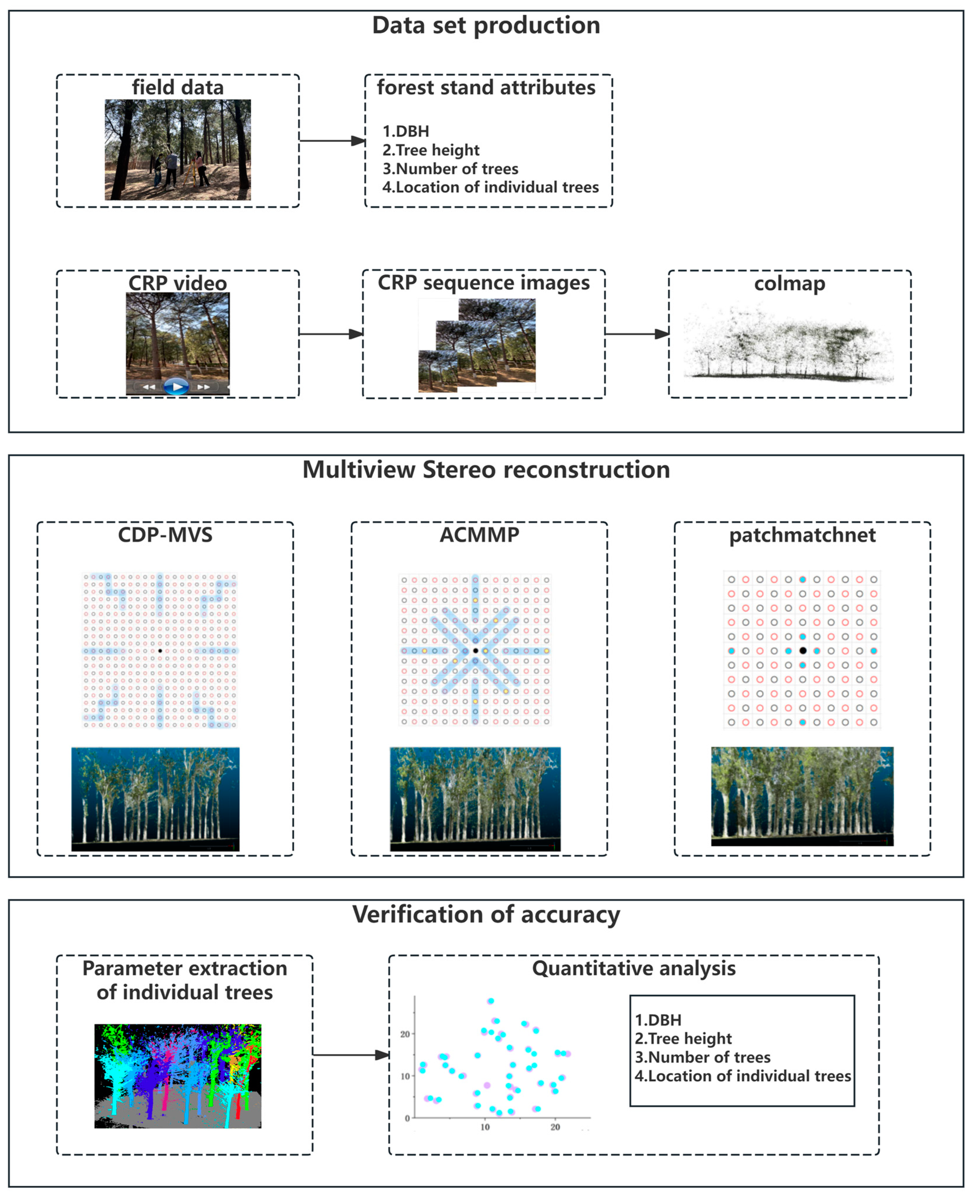
Figure 3 illustrates the overall workflow of this study, encompassing three main modules: (1) Dataset Construction: This includes the field measurement of individual tree parameters, extracting sequence images of the plots from video frames, and using the Colmap algorithm to recover camera poses. (2) Multi-View Reconstruction: We employed three block-matching-based models to generate visualized point clouds of the forest plots. Among these, CDP-MVS is an improved version of the traditional multi-view reconstruction model ACMMP, both of which are block-matching-based traditional methods. In contrast, PatchMatchNet is a deep learning-based block-matching model, used for comparative analysis with the other two. (3) Accuracy Validation: Since the point clouds generated by multi-view reconstruction lack scale, we first used CloudCompare software (v2.13) to calibrate the point clouds with known-size references in the plots. We then utilized LiDAR360 software (v6.0.3.0) for individual tree segmentation and parameter extraction. Finally, we compared the parameters extracted from the point clouds with the field measurement data and presented the corresponding visualization results.

2.2.1. Dataset Creation

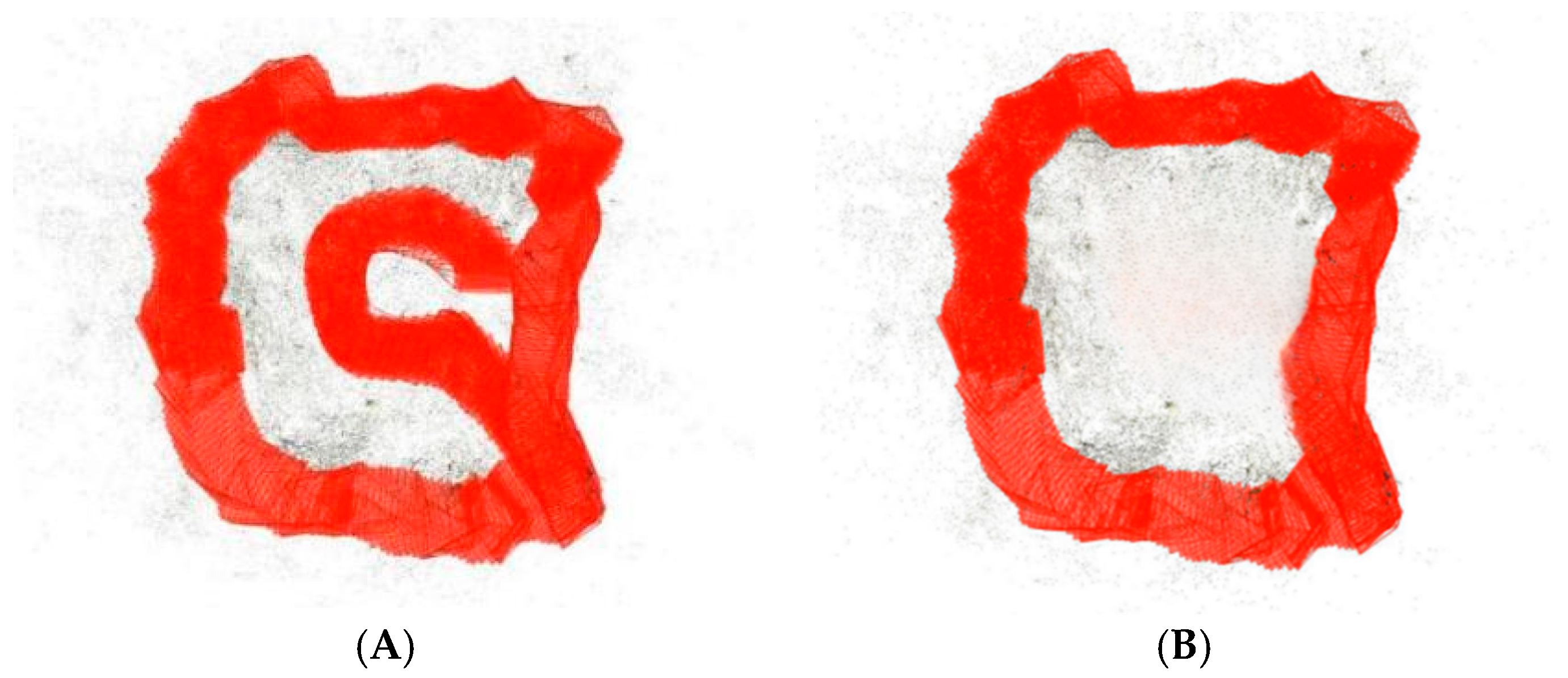
We successfully completed the field measurements and video recordings within the study area. Subsequently, we developed a script to extract and label frames from the videos, removing redundant and blurred frames, and ultimately produced a high-quality sequence of plot images. The frame extraction frequency was positively correlated with the tree density, canopy size, and vegetation complexity of the plots. The number of extracted images for poplar, pine, and elm plots was 278, 164, 394, and 293, respectively, providing essential baseline data for subsequent reconstructions. We then employed the Colmap algorithm to perform sparse reconstruction on the image sequences generated by the two filming methods. The obtained camera pose information will be used in the next step for multi-view reconstruction, while the generated sparse point clouds will be used to evaluate the impact of different filming methods on reconstruction quality. Clearly, the new filming method demonstrated greater advantages in point cloud reconstruction, resulting in a higher level of completeness in the generated point clouds (as shown in Figure 4). This improvement is primarily attributed to the additional circular path within the plot, which successfully supplemented the previously missing central forest plot viewpoints, thereby effectively reducing reconstruction bias caused by tree occlusion or excessive camera distance. Moreover, compared to the traditional method of fixed-point filming, the new video recording method is not only more time-efficient, typically completing the required image capture for a plot within two to six minutes, but also provides a sufficient number of frames for selection, eliminating concerns about missing viewpoints due to the removal of blurred images. Additionally, we can flexibly adjust the frame extraction frequency according to the complexity of the forest plot, which not only resolves the issue of image redundancy but also ensures the completeness of reconstruction viewpoints, providing strong support for high-precision 3D reconstruction.

2.2.2. Multi-View Reconstruction

The multi-view reconstruction problem in this paper is formulated as follows: Given a set of input images I = {Ii|i = 0…N − 1} and their corresponding camera parameters P = {Pi|i = 0…N − 1}, the block-matching-based reconstruction algorithm iteratively selects an image as the reference image Iref, while the remaining images form the source image set Isrc = I − Iref. The depth and normal of the reference image Iref are then recovered through guidance from the source images [14].
To validate whether the dense point clouds generated by the block-matching-based multi-view reconstruction algorithm meet the requirements for extracting individual tree parameters, we will explore three block-matching-based reconstruction algorithms: ACMMP, CDP-MVS, and PatchMatchNet. Typically, block-matching reconstruction algorithms include four key steps: initialization, propagation, evaluation, and refinement. After initialization, the algorithm iterates through the latter three steps until convergence. We will first review and analyze ACMMP in detail, as it is a state-of-the-art algorithm. In the CDP-MVS algorithm section, we will delve into its improvements over ACMMP, while in the PatchMatchNet section, we will investigate the differences introduced by deep learning-based methods compared to traditional approaches.
i.
ACMMP
The ACMMP algorithm takes multi-view images and their corresponding camera parameters as inputs and outputs the depth maps and normal maps of these images. The algorithm first constructs a multi-scale model and performs depth estimation with plane priors at each scale to reduce errors in low-texture areas. However, since plane prior estimation is still based on photometric consistency, it inevitably introduces some erroneous point estimates. To address this issue, the algorithm employs multi-scale geometric consistency depth estimation optimization to improve erroneous depth estimates. The depth estimation steps of the ACMMP algorithm are as follows:
(1) Initialization:
ACMMP generates a random initial plane hypothesis for each pixel in the reference image Iref. This hypothesis is then matched with the source image set Isrc, and the matching cost for each pixel under this hypothesis is calculated to assess the reliability of the plane hypothesis.
(2) Propagation:
ACMMP improves upon the sampling method of the Gipuma [26] algorithm by expanding the sampling area of neighboring plane hypotheses from eight points to four V-shaped regions and four strip regions, essentially still using fixed-area sampling. Based on multi-view matching costs, in each of the eight regions, the plane hypothesis with the minimum cost is selected as a candidate hypothesis (as shown in Figure 5).
(3) Multi-View Matching Cost Calculation:
This section’s formulas are derived from a summary of the paper ACMMP [14]. In the reference image Iref, for each pixel p, the matching costs between all adjacent views are calculated. The eight candidate plane hypotheses obtained during propagation are then embedded into the cost matrix M. The column vector represents the eight depth plane hypotheses, while the row vector corresponds to the N − 1 source images.
M = m 0 , 1   m ( 0 , N 1 ) m ( 1,1 )   m ( 1 , N 1 )             m 8,1   m ( 8 , N 1 )
Due to the potential impact of unreliable views on the accuracy of depth estimation, ACMMP sets thresholds within the cost matrix to filter out a reliable subset of neighboring views (St). The good view cost threshold is defined as τ ( t ) . When the matching cost of a view is less than τ ( t ) , it is included in the good view subset S good . Conversely, the bad view cost threshold is defined as a constant τ b , and when the matching cost of a view exceeds τ b , it is classified into the bad view subset S bad . The threshold τ ( t ) is related to the iteration number t, and its formula is
τ t = τ i n i t e t 2 u
Here, τ i n i t represents the initial view cost threshold, and both τ i n i t and u are constants.
Constants n 1 and n 2 are defined, and the selected view set St is as follows:
S t = { I j | I j   I src     | S good ( j ) |   >   n 1     | S bad ( j ) |   <   n 2 }
The matching cost is then used to calculate the confidence of the selected views, thereby quantifying the reliability of each view. The confidence formula is as follows, where β is a constant:
C ( m i , j ) = e m i , j 2 2 β 2
Assign the initial weight to the source view Ij based on the confidence.
ω init I j = 1 S g o o d j m i , j S g o o d j C m i , j ,                                             i f   I j S t ; 0 ,                                                                                                                             e l s e .  
The view with the highest weight in the previous iteration v t 1 influences the view selection in the current iteration. Thus, the weight of the view during iterative propagation is defined as follows:
ω j = ( II ( I j = v t 1 ) + 1 ) ω i n i t ( I j ) ,               i f   I j S t ; 0.2 II ( I j = v t 1 ) ,                                                     e l s e .
II (*) is an indicator function, where II (*) =1 if * = true and II (*) = 0 if * = false.
The multi-view matching cost based on photometric consistency is defined as
m g e o ( p , θ i ) = j = 1 N 1 ω j m i , j j = 1 N 1 ω j
Furthermore, ACMMP also introduces planar priors and geometric consistency into the calculation of matching costs, further improving the accuracy of depth estimation.
(4) Refinement
After completing the above three steps, randomly perturbed plane hypotheses are added to the set of plane hypotheses for each pixel. The hypothesis with the lowest multi-view matching cost is then selected as the final plane hypothesis, further improving the accuracy of depth estimation [29].
ii.
CDP-MVS
In ACMMP’s block-matching dense reconstruction, the sampling propagation method merely extends the original eight points into eight elongated regions, but essentially, it still conducts sampling within a fixed area. This method’s depth values are overly dependent on local information, making geometric recovery susceptible to low-texture areas, and expanding the fixed sampling area may potentially waste computational resources. To ensure the efficiency of the algorithm while finding more reliable depth hypothesis planes, we employed a non-local dynamic domain propagation sampling mode. This allows the algorithm to selectively expand the sampling area based on the reliability of each sampled depth. Furthermore, the previous cost evaluation method, based on normalized cross-correlation with bilateral filtering, only considered photometric consistency. This approach tends to generate ambiguous regions during forest reconstruction under uneven lighting and mutual occlusion. Therefore, this paper proposes a new confidence calculation method that quantifies the reliability of the selected views from multiple aspects, including depth error, geometric error, and matching cost. Guiding the propagation sampling with this new confidence measure leads to more accurate depth estimation. Lastly, images of forest plots captured from close range often contain a significant amount of sky in the background, which interferes with depth estimation, especially for tree canopies. To address this, during the depth map fusion stage, we binarized the grayscale reference images, marking the sky regions as 0 and other regions as 1. These binarized images were then matched with the depth maps, setting the depth values in the sky regions to 0. This approach effectively reduces noise in the fused point clouds.
(1) Dynamic Domain Propagation Mode
A reasonable propagation mode is crucial for sampling depth hypotheses, as it is a prerequisite for cost evaluation. Early diffusion propagation algorithms, like Gipuma, sample depth hypotheses at eight fixed points around the pixel to be estimated. ACMMP, on the other hand, proposes sampling depth values within eight linear regions, selecting the point with the minimum matching cost in each region as the candidate depth hypothesis. Essentially, both methods rely on sampling within fixed areas. Gipuma does not assess the reliability of the depth hypotheses when sampling at the eight points, introducing a certain level of randomness. Although ACMMP introduces reliability assessment for depth hypotheses, expanding the fixed sampling areas also increases the algorithm’s time complexity. In contrast, CDP-MVS adopts a dynamic domain sampling propagation strategy. It sets two propagation cost thresholds, selecting the point with the lowest matching cost in the eight linear regions as the candidate hypothesis. The process of expanding the sampling area stops when the view cost of the sampling point meets the cost threshold or reaches the maximum propagation extension count. Additionally, the sampling area is decentralized, effectively preventing the estimated depth values from becoming trapped in local optima. CDP-MVS defines the good propagation cost threshold as τ ( t i t e r , t m a x ) , and the bad propagation cost threshold as a constant τ p-b . The threshold τ ( t i t e r , t m a x ) is related to the number of expansions, and its formula is as follows:
τ t i t e r , t m a x = β e α t i t e r 2 ( t m a x t i t e r )
Here, α and β are constant coefficients. tmax is the maximum number of extensions, and titer is the current number of extensions.
Constants ngood and nbad are defined such that, for the pixel being estimated, at least ngood propagation costs must not exceed τ ( t i t e r , t m a x ) , and at most nbad propagation costs may exceed τ p-b . If these conditions are not met, the area will be expanded, doubling the number of sampling points.
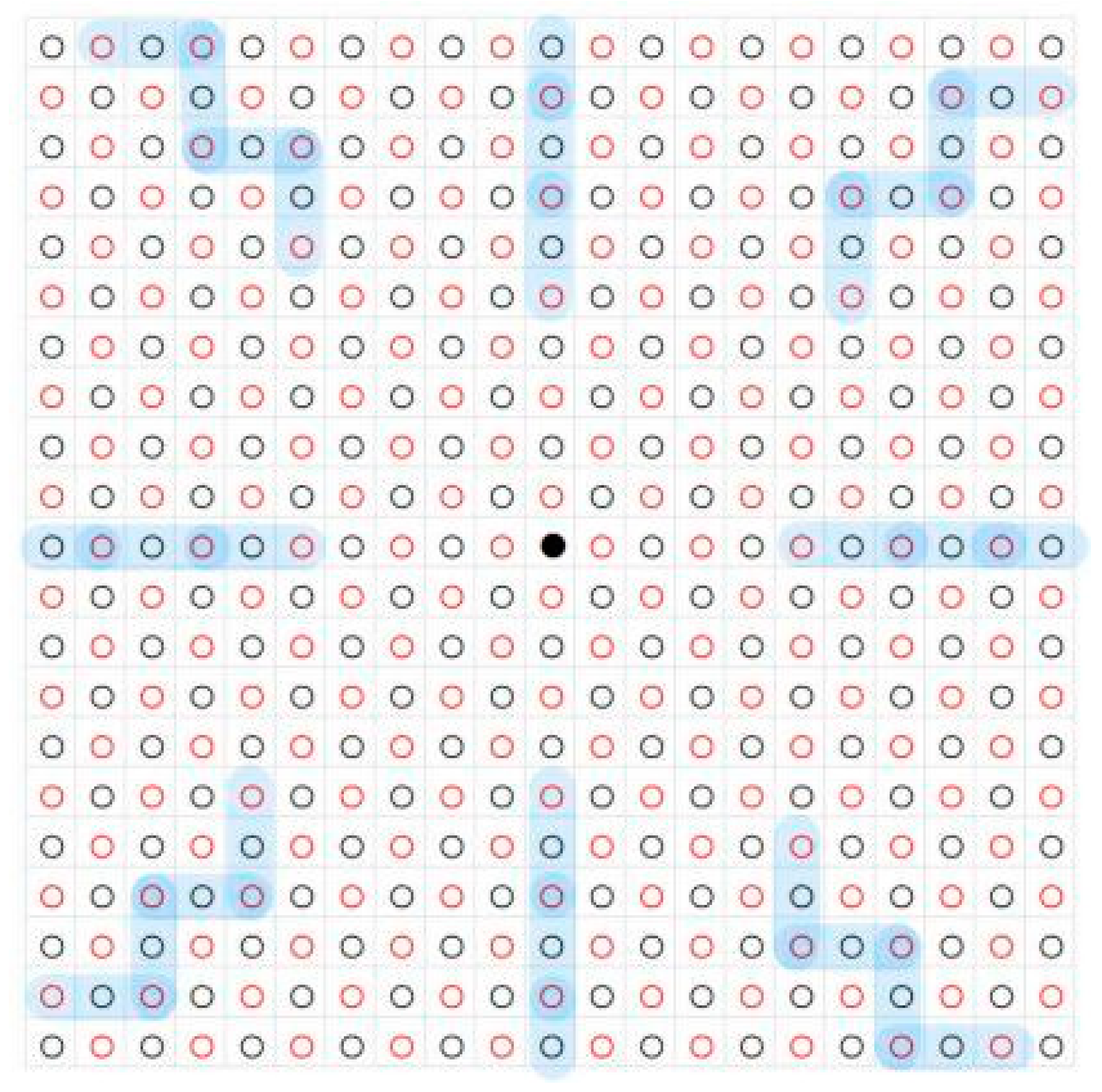
For forest land reconstruction, we set three expansion opportunities per iteration, with each expansion sampling five points. These five points are equidistant and extend further as the number of iterations increases. During each expansion, the point with the minimum cost is selected. If the position of the minimum cost point is updated, the depth hypothesis is updated, and the multi-view matching cost matrix in this direction is recalculated (as shown in Figure 6).
(2) Enhanced Confidence
Confidence is an assessment of the reliability of matching results, reflecting the accuracy of depth hypotheses and helping in the selection of good view subsets. Low-confidence depth hypotheses are considered erroneous and need to be filtered or refined later, while high-confidence depth hypotheses accurately reflect the true surface of the object being estimated [30]. Generally, the confidence of depth hypotheses in algorithms is entirely determined by the matching cost based on photometric consistency. However, during the evaluation stage, due to the limited identifiable information in low-texture areas, the matching costs based solely on photometric consistency are very close in these regions, making it easy for incorrect plane hypotheses to be selected. To address this issue, ACMMP adds geometric consistency and plane prior constraints to assist in generating multi-view matching costs, thereby reducing incorrect plane hypotheses in low-texture areas. Reference [31] attempts to eliminate incorrect plane hypotheses by adding local consistency constraints. While photometric consistency effectively characterizes objects or scene structures in structured environments, adding constraints to the matching cost can indeed help mitigate the issue of ambiguous matches in low-texture areas to some extent. However, new constraints may blur geometric details in objects or scenes. Moreover, these constraints are still fundamentally based on photometric consistency, addressing the symptoms rather than the root cause of ambiguous matching. Therefore, the newly defined comprehensive confidence measure no longer adds additional constraints to the matching cost. Instead, it evaluates the reliability of matching views from multiple perspectives, beyond just photometric consistency, to obtain a new comprehensive confidence measure. The new confidence is composed of multi-view confidence and patch confidence.
Reprojection error refers to the difference between the point projected from the reconstructed three-dimensional model and the corresponding observed point in the image (as shown in Figure 7). If we know the pixel (p) on the reference image (Iref) and its plane hypothesis, Φp (dp, np), the reprojected point (p’) and the reprojected plane, Φp′ (dp′, np′), in the image can be calculated through the projection matrix. Then, by comparing these reprojected results with the actual observed results, the magnitude of the reprojection error can be determined [32]. Based on this, we define the formulas for geometric confidence ( N geo ), depth confidence ( N d ) and cost confidence ( N c ) as follows:
N d = e 1 σ d 2 d p d p d p 2
N geo = e p p 2 σ g e o 2
N c = e m ( i , j ) 2 σ c 2
The multi-view confidence can thus be defined as
N m u l t i v i e w = i = 1 N 1 N c N d N g e o N 1
Patch confidence is determined internally by the reference image. The PatchMatch algorithm assumes that the depth values of neighboring pixels tend to converge, allowing pixels within a patch to share the same plane hypothesis. Based on this principle of local plane consistency, we propose patch confidence, which complements multi-view confidence to form the final confidence measure. Patch confidence is calculated in four directions based on the depth value deviation between the pixel to be estimated and its neighboring pixels. For example, the confidence for the left neighboring pixel is calculated as
N l e f t = e D r e f D l e f t D r e f
Similarly, the confidence for the other three directions—Nright, Nup and Ndown—is calculated. The final patch confidence is then determined as
N p a t c h = N l e f t N r i g h t N u p N d o w n
The final comprehensive confidence is given by
N final = N m u l t i v e i w N p a t c h
(3) Confidence-Guided Dynamic Domain Propagation
The dynamic domain propagation mechanism aims to sample highly reliable depth hypotheses from surrounding pixels as the depth value for the pixel being estimated. The criteria for determining the sampling area and depth hypotheses are based on multi-view matching costs. However, in low-texture regions where identifiable information is sparse, the matching costs calculated for different plane hypotheses are similar, reducing the probability of selecting the correct plane hypothesis and making it difficult to determine whether to expand the sampling area. As a result, it is challenging to replace incorrect depth estimates through the propagation mechanism. These incorrect depth estimates often exhibit low confidence. In the previous sections, we altered the propagation mode to efficiently select more reliable depth hypotheses and defined a new confidence metric as a quantitative standard for the accuracy of depth hypotheses. By integrating this newly defined confidence into the calculation of multi-view matching costs, the probability of selecting the correct plane hypothesis is increased, thereby achieving confidence-driven dynamic domain propagation. The new multi-view matching cost is defined as
m p , θ i = j = 1 N 1 ω j · m p , θ i + λ · 1 N final p , θ i j = 1 N 1 ω j
The modified multi-view matching cost introduces a confidence factor, with confidence being inversely proportional to the matching cost. In low-texture regions, where photometric consistency-based matching costs are often unreliable, confidence is typically lower. However, this lower confidence gives the confidence factor greater weight in the multi-view matching cost, effectively reducing the influence of unreliable matching costs. Additionally, since the multi-view matching cost is a key condition for the expansion of the sampling domain, incorrect planes with low confidence are usually replaced by correct hypothesis planes during the dynamic expansion process due to their higher matching costs. In texture-rich regions, pixel confidence is generally higher, and the photometric consistency-based matching cost is also more reliable. High-confidence pixels, due to their lower matching costs, can more easily propagate to other pixel regions, even reducing the number of dynamic domain expansions needed. Therefore, confidence-guided multi-view matching costs exhibit different advantages across various texture regions, potentially reducing propagation time and improving the accuracy of depth estimation.
To avoid the complexity of repeated confidence calculations due to changes in plane hypotheses, confidence-based depth estimation is limited to obtaining the final depth map through a single propagation. This confidence-based depth estimation method ensures that the final depth map not only preserves structural details well but also significantly improves the estimation quality in low-texture regions.
(4) Image Segmentation to Remove Sky Information
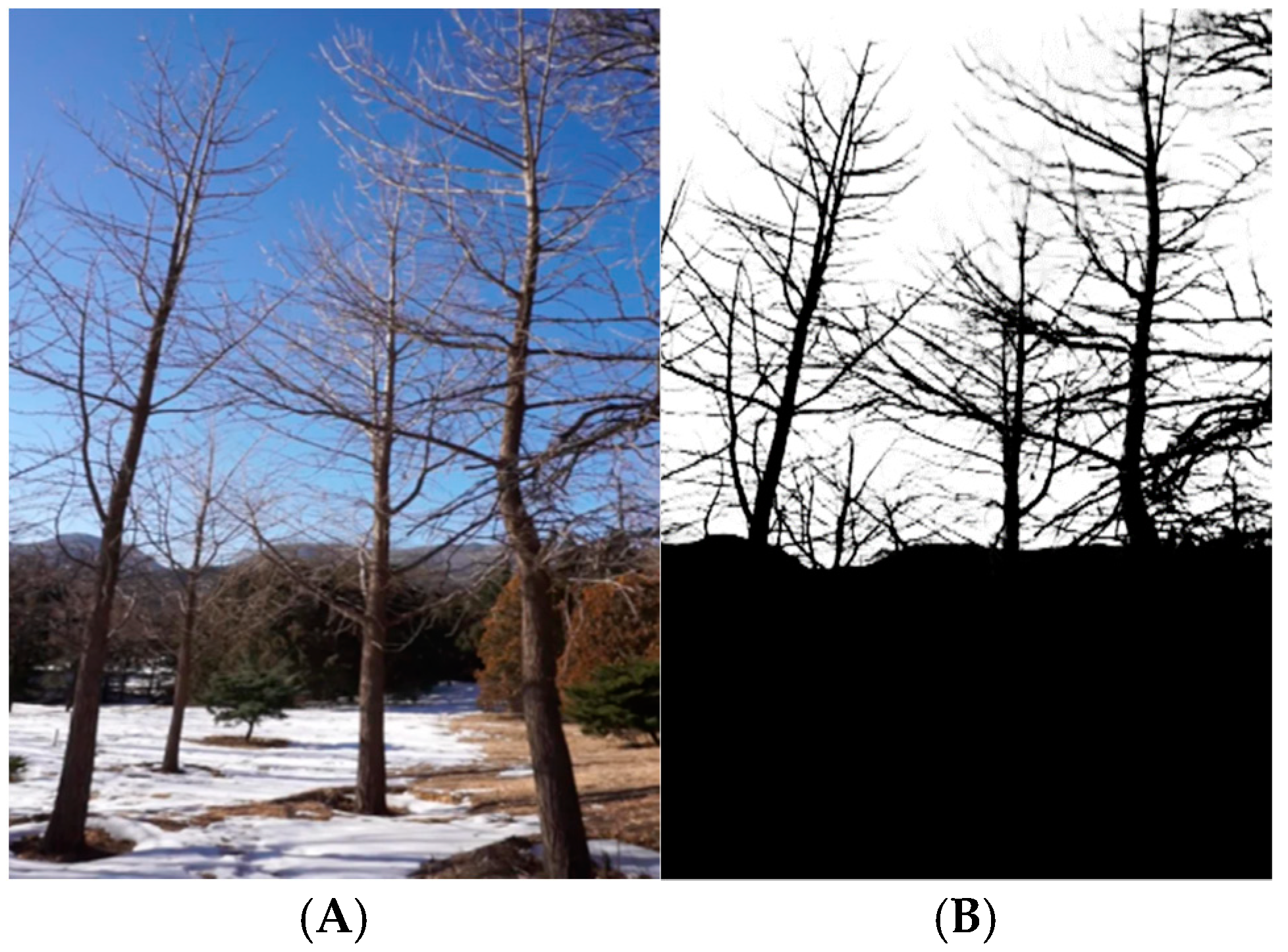
In block-matching algorithms, depth hypotheses are gathered from surrounding pixels, but the depth value of the sky is infinite and cannot be accurately estimated. These incorrect depth values can spread and merge with the depth values of nearby branches, ultimately causing these values to become very close to those of the surrounding canopy. As a result, the reconstructed canopy often contains incorrect sky information, leading to noise that severely impacts the visualization of forest land. To address this issue, we binarized the grayscale reference images, setting a threshold at a pixel value of 150 to segment the sky regions. These segmented sky regions were then matched with the corresponding depth maps, with the depth values in the identified sky regions set to 0. This approach ensures that the resulting depth maps, when fused, contain minimal sky-related noise in the point cloud. Figure 8 illustrates a ginkgo forest captured in the National Botanical Garden during the winter of 2023, where the selected forest plot has extremely fine branches and a significant amount of sky in the background. Despite this, the binarized grayscale images used for sky segmentation retained the completeness and clarity of the branches.
(5) Multi-Scale Layered Exploration
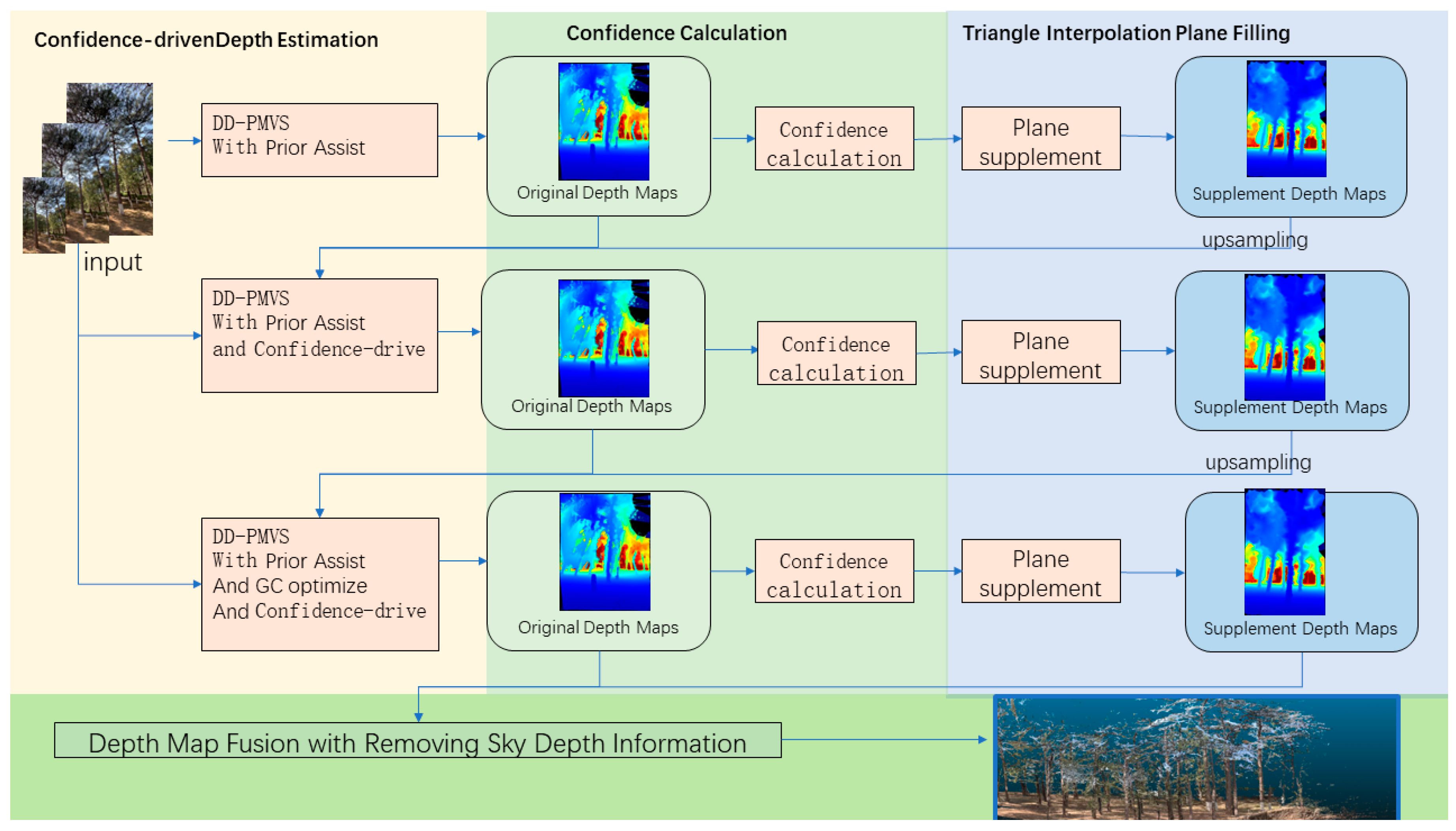
As shown in Figure 9, high-confidence pixels typically contain rich texture information and geometric structures, making the depth hypotheses extracted from these regions highly accurate and reliable. These pixels can effectively guide the depth estimation optimization in neighboring low-confidence areas. Therefore, after calculating the confidence of the plane hypotheses, we extract high-confidence pixels (with a confidence threshold set at 0.8) from the coarse depth map. The extracted high-confidence pixels serve as anchor points, and the image is segmented into triangular elements of varying sizes using Delaunay triangulation [29]. A local 3D plane is then constructed based on the depths of the three anchor points forming each triangular element. Low-confidence pixels within each triangular element are projected onto the local 3D plane to obtain new depth values, thereby generating an additional supplemental depth map.
In edge regions, the confidence of the coarse depth map, which relies on photometric consistency, is higher than that of the supplemental depth map. Conversely, in low-texture regions, the supplemental depth map shows greater confidence than the coarse depth map. Therefore, after generating the supplemental depth map, we recalculate the confidence of the plane hypotheses in the supplemental depth map and then compare them with the coarse depth map, retaining the plane hypotheses with higher confidence to assist in the next stage of depth estimation.
CDP-MVS retains the multi-scale layered exploration framework from ACMMP for depth information extraction, with the dynamic domain propagation block-matching algorithm named DD-PMVS, serving as the core module of CDP-MVS. Additionally, CDP-MVS includes a new confidence calculation module, a supplemental depth map comparison module, and a sky noise removal depth map fusion module. These three modules collectively form the layered exploration architecture, further enhancing the accuracy and robustness of depth estimation.
iii.
PatchMatchNet
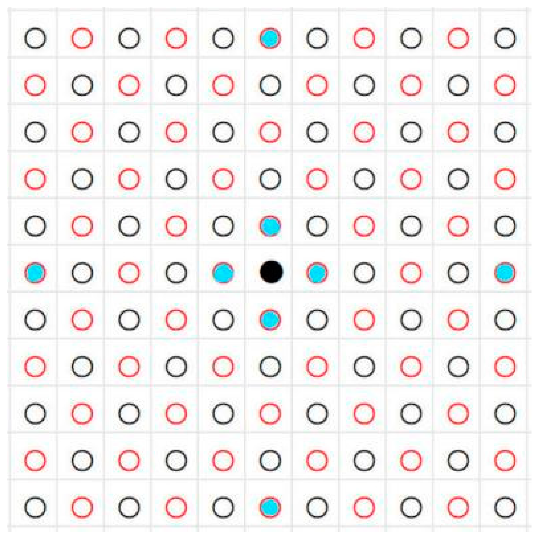
PatchMatchNet is the first to implement a multi-scale block-matching multi-view reconstruction deep learning network within an end-to-end training framework. It leverages neural networks to extract image features and enhances traditional block-matching propagation and cost evaluation steps with a learnable adaptive module, making it a trade-off between runtime and accuracy. Specifically, PatchMatchNet is a cascade structure with learning-based PatchMatch as the main body. It mainly includes multi-scale feature extraction based on FPN, learning-based PatchMatch embedded in the cascade structure, and a spatial refinement module (used for upsampling to the original image size). For the propagation mode, it adopts a fixed sampling strategy with eight points, as shown in Figure 10. Since PatchMatchNet is a model trained through deep learning, its robustness heavily depends on the quality and diversity of the training data. Its generalization ability is not as strong as that of traditional reconstruction algorithms [33].

2.2.3. Accuracy Validation

After completing the multi-view reconstruction, we obtained unscaled point clouds for nine plots. We selected reference objects within the plots and measured their actual sizes, then used CloudCompare software for calibration to acquire the true dimensions of the point cloud plots. Subsequently, we utilized LiDAR360 software to extract individual tree parameters from the dense point clouds, which involved steps such as denoising, ground point classification, ground point normalization, and individual tree segmentation. Finally, the extracted parameter values were compared and quantitatively analyzed against the field survey measurements. The quantitative metrics included reconstruction quantity accuracy (QAE), DBH accuracy (DAE), average Euclidean distance of tree positions (AED), and tree height accuracy (HAE). The formulas for the quantitative metrics are as follows:
Q A E = 1 N e x t r a c t i o n N t r u t h N t r u t h × 100 %
D A E = 1 i = 1 N t r u t h D e x t r a c t i o n D t r u t h D t r u t h n × 100 %
  A E D = 1 N t r u t h i = 1 N t r u t h ( X e x t r a c t i o n X t r u t h ) 2 ( Y e x t r a c t i o n Y t r u t h ) 2
      H A E = i = 1 N t r u t h H e x t r a c t i o n H t r u t h H t r u t h × 100 %

3. Results

3.1. Visualization Results

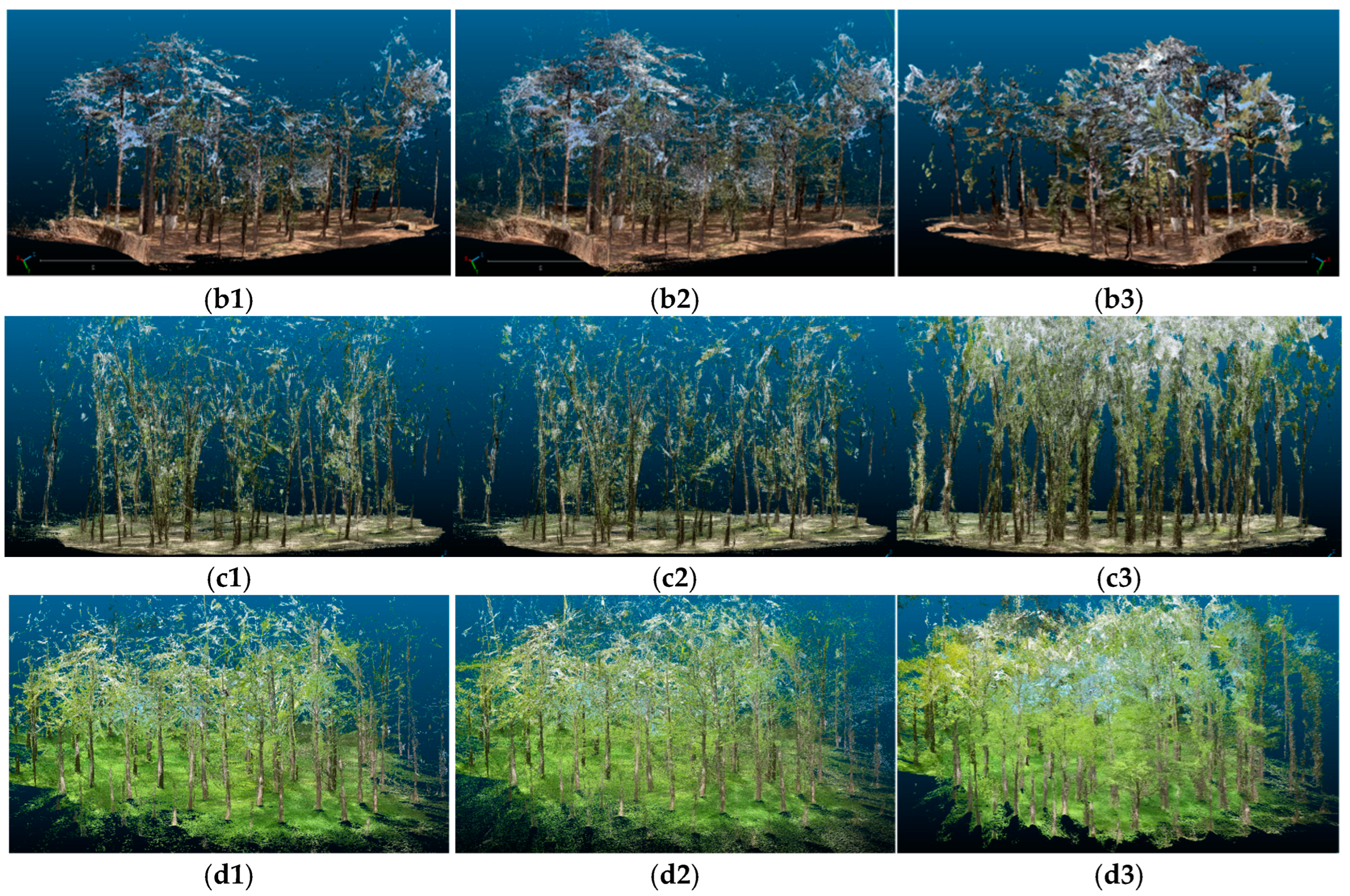
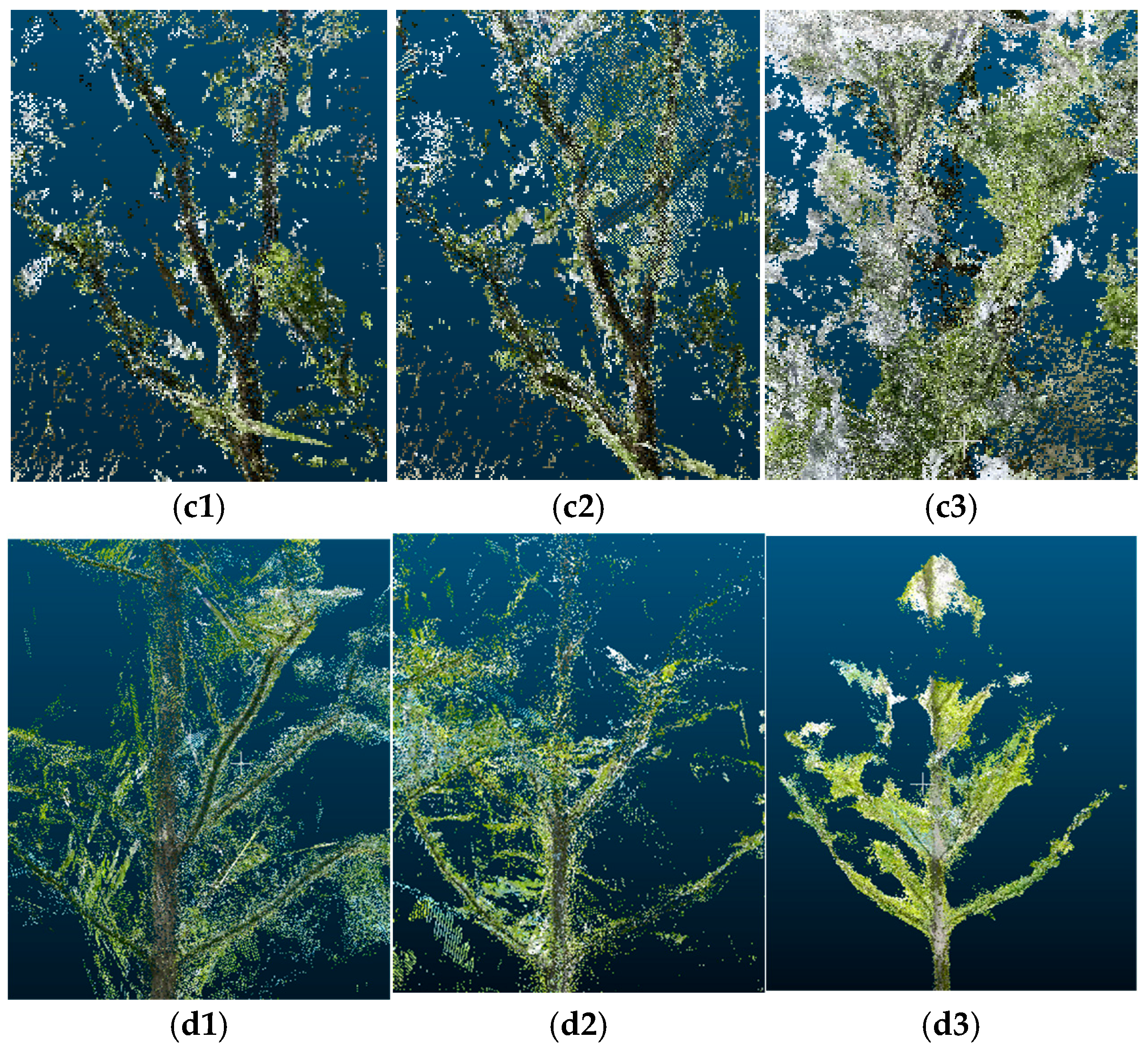
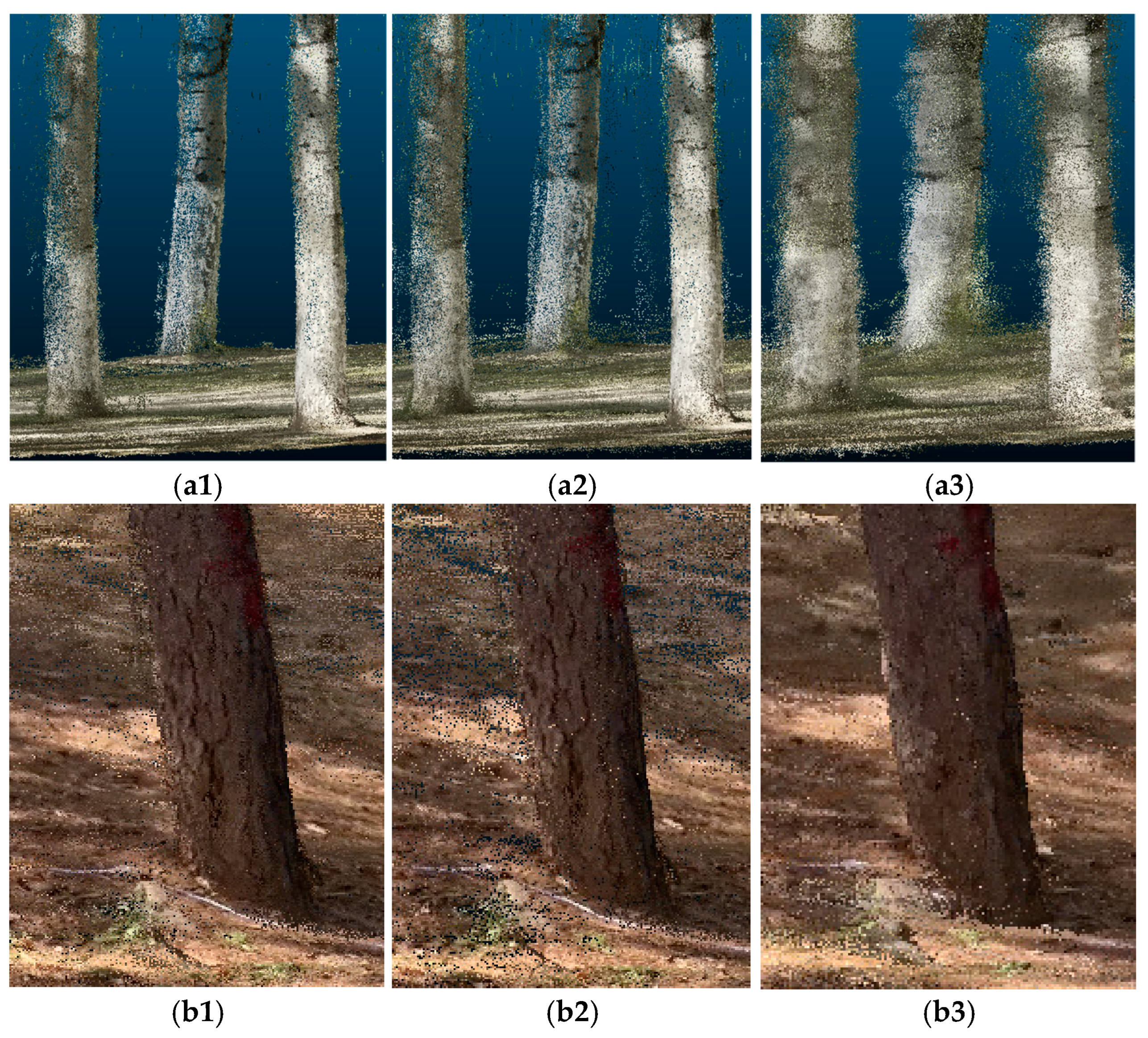
We compared the denoised point cloud visualization results across the plots (as shown in Figure 11). The point clouds reconstructed by PatchMatchNet exhibited dense and erroneous sky information in the canopy regions across all three plots, with almost no detailed branch structure. In contrast, CDP-MVS showed the least sky interference around the canopy, with the clearest and most complete branch reconstruction (as shown in Figure 12). For the trunk regions (as shown in Figure 13), CDP-MVS again outperformed the others, with fewer noise points and clearly defined trunk edges, free of ghosting, laying a solid foundation for subsequent extraction of individual tree DBH values.

3.2. Reconstruction Time Performance

Table 2 shows the runtime of different algorithms for reconstructing the three plots (measured in hours). In terms of reconstruction time, CDP-MVS offers a slight improvement over ACMMP. This enhancement is due to the dynamic domain propagation method, which enables the algorithm to find the correct depth estimates quicker, leading to fewer iterations and faster convergence. The deep learning-based PatchMatchNet model consumes the most computational resources, with reconstruction times far exceeding those of the other two algorithms. It is challenging to bridge this significant runtime gap by simply altering the neural network structure. This demonstrates that traditional algorithms still hold significant, irreplaceable advantages, particularly in terms of runtime and resource consumption.

3.3. Reconstructed Tree Quantity

In terms of the number of reconstructed trees (as shown in Table 3), CDP-MVS achieved zero-error reconstruction across all three plots, improving accuracy by 6.25%, 0%, 7.89% and 8.7% compared to ACMMP. This improvement is attributed to the new confidence measure, which effectively mitigates the issue of feature point mismatches caused by uneven lighting in forest plots, significantly reducing the probability of tree duplication in the model. Due to ACMMP’s use of geometric consistency and plane priors in depth estimation, it also outperforms PatchMatchNet in terms of reconstruction quantity accuracy.

3.4. Reconstructed Tree Positions

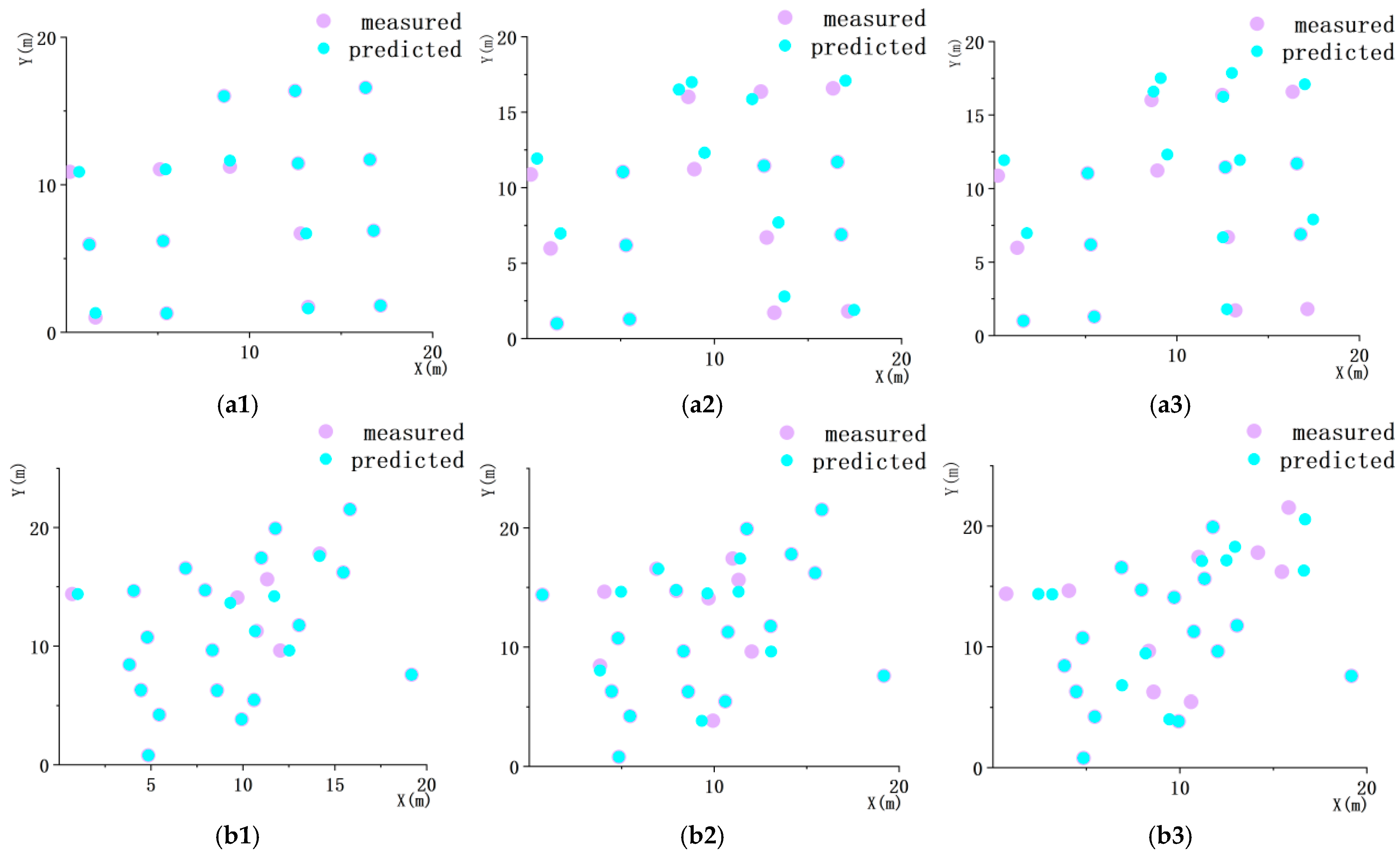
We manually removed duplicated trees to facilitate the quantitative analysis of position deviation, DBH deviation, and tree height deviation. Overall, the reconstruction accuracy is higher at the edges of the forest plots, with a lower probability of tree duplication (as shown in Figure 14). Among the different models, the Euclidean distance deviation between the reconstructed tree positions and the actual positions is smallest for CDP-MVS, converging within 0.25 m (as shown in Table 4). The position deviations for individual trees reconstructed by PatchMatchNet are larger in all plots compared to the other two algorithms.

3.5. Reconstructed Tree DBH

Table 5 shows the accuracy of reconstructed tree DBH. In terms of DBH accuracy, CDP-MVS improved the reconstruction precision by 0.42%, 0.24%, 2.09% and 3.37% compared to the ACMMP algorithm, which is within the measurement error range. The reconstruction accuracy of DBH of the three models meets our research requirements. However, in the pine plot, PatchMatchNet achieved the highest reconstruction accuracy, surpassing CDP-MVS by 3.78%. The average DBH values reconstructed by CDP-MVS and ACMMP were slightly lower than the measured DBH, whereas PatchMatchNet’s results were slightly higher than the measured values. This highlights the differences between the two types of algorithms.

3.6. Reconstructed Tree Height

As shown in Table 6, In terms of tree height, all models produced point clouds with tree heights lower than the actual measurements. The errors in tree height extraction between ACMMP and CDP-MVS were relatively close. There was no significant advantage or disadvantage among the three models across different plots. It is worth noting that as the actual tree height increases, the absolute deviation of all reconstruction models also increases. This indicates that close-range photogrammetry, due to the lack of overhead perspectives of forest trees, can only ensure accuracy for trees under ten meters in height. Among the tree species in our research, this defect currently cannot be overcome without providing additional data sources.

4. Discussion

Based on close-range photogrammetry, we designed a semi-automated method for generating forest plot image sequences and explored an efficient and accurate multi-view reconstruction algorithm. The new image sequence generation method effectively eliminated the negative impact of slope on image acquisition. The new multi-view reconstruction algorithm, CDP-MVS, successfully addressed issues such as tree duplication, prolonged reconstruction times, and unclear canopy reconstruction. The feasibility is demonstrated in four typical types of artificial forests in China. The high-quality point cloud data generated meet the requirements for forest plot visualization and accurate extraction of tree parameters.

4.1. Impact of Different Terrains on Reconstruction Results

Previous studies have suggested that steep plot slopes can negatively affect reconstruction results. This is primarily due to the difficulty in maintaining the stability of imaging equipment when moving across steep slopes, resulting in a higher proportion of blurred images, which are challenging to detect and retake in the field. Additionally, when capturing images of steeper plots from the same horizontal distance, the extra vertical movement reduces the overlap between images from different perspectives, hindering effective reconstruction. These factors typically lead to a negative correlation between reconstruction accuracy and plot slope. However, our newly proposed image sequence generation method effectively resolves this issue. First, forest plot videos provide a large number of frames for selection and extraction, allowing us to discard blurred and overexposed frames while still ensuring sufficient image overlap. Additionally, we can freely adjust the frame rate to ensure time efficiency during the reconstruction process. In our experiments, terrain factors did not significantly impact the reconstruction results. This indicates that the influence of terrain on reconstruction outcomes can be mitigated through the new image sequence generation method.

4.2. Comparison between Traditional Block-Matching Geometric Reconstruction Models and Deep Learning Models

Although deep learning-based reconstruction algorithms perform exceptionally well on small-scale datasets like DTU, traditional algorithms significantly outperform deep learning models in more challenging large-scale scenarios, such as ETH3D. From the results of forest land reconstruction, traditional algorithms demonstrate clear advantages in reconstruction time, canopy clarity, and reducing tree duplication compared to deep learning models. This disparity can be attributed to three main factors.
First, traditional algorithms consume fewer computational resources, whereas deep learning models require processing a vast amount of high-dimensional features and cost volumes, leading to extremely high computational complexity and significant GPU resource demands during inference. Second, traditional algorithms are highly flexible and can be manually adjusted to address specific issues in forest land, such as feature point mismatches caused by uneven lighting. These algorithms can modify matching costs and confidence calculations, incorporating geometric consistency and local coherence constraints to effectively mitigate such problems. In contrast, algorithms that rely on neural networks to automatically learn features and matching strategies have a black-box nature, preventing the manual addition of specific constraints. Additionally, this black-box nature means that the performance of deep learning models is highly dependent on the quality and diversity of the training data. If the training data do not cover all possible variations in the scenes, the model’s generalization ability will be limited, making it difficult to adapt to complex situations in new environments. Therefore, deep learning models exhibit clear limitations when dealing with complex and dynamic scenes like forest land.

4.3. Research Limitations

Close-range photogrammetry videos, due to the lack of overhead perspectives, are not conducive to accurate tree height reconstruction. In future filming, we need to extend the camera’s distance and elevate it to alleviate this issue. Currently, ACMMP shows excellent reconstruction performance in large-scale urban scenes captured by drones. In the future, the improved CDPMVS algorithm will be applied to videos captured by drones of forest plots for reconstruction, which is expected to generate higher-quality visualized point clouds and achieve more accurate parameter extraction.

5. Conclusions

To obtain clear images with high overlap and no redundant photos in forest plot image sequences, we used frame extraction from videos. To improve the accuracy of sparse reconstruction, we explored capturing forest plots using a two-circle method. The results showed that the completeness of sparse point clouds obtained with the two-circle method was higher than with the single-circle method. Additionally, we proposed an improved algorithm, CDP-MVS, to address the specific challenges of forest land. The algorithm introduces a new comprehensive confidence measure and multi-view matching cost calculation to address feature point mismatches caused by uneven lighting, achieving a 100% accuracy rate in tree reconstruction. To tackle the issue of excessive sky information in forest plots, the algorithm removes sky depth values during the depth map fusion stage, resulting in clearer and less noisy canopy reconstructions. Furthermore, the algorithm employs a decentralized dynamic domain propagation sampling method, enhancing the reliability of each sampled depth hypothesis and speeding up convergence, resulting in a slight improvement in time efficiency compared to CDP-MVS.

Author Contributions

Z.L. conducted the experiments and wrote the manuscript. S.C. edited the manuscript, and both contributed to field data collection in forestland. X.Z. provided guidance in planning the experimental design. Z.C. supervised the work and revised the manuscript. All authors have read and agreed to the published version of the manuscript.

Funding

This research was funded by the National Key Research and Development Program of China: Intelligent Forest Field Observation Equipment and Precision Extraction Technology for Tree Parameters, grant number 2023YFD2201701.

Data Availability Statement

As the data were collected by multiple individuals and involve privacy concerns, they are not publicly available. However, the algorithm model used in the paper has been made available on Gitee.

Acknowledgments

We would like to thank Dianchang Wang, Lishuo Huo, and Lingnan Dai for their contributions to data collection.

Conflicts of Interest

The authors declare no conflicts of interest.

References

  1. You, L.; Tang, S.; Song, X.; Lei, Y.; Zang, H.; Lou, M.; Zhuang, C. Precise Measurement of Stem Diameter by Simulating the Path of Diameter Tape from Terrestrial Laser Scanning Data. Remote Sens. 2016, 8, 717. [Google Scholar] [CrossRef]
  2. Zhu, R.; Guo, Z.; Zhang, X. Forest 3D Reconstruction and Individual Tree Parameter Extraction Combining Close-Range Photo Enhancement and Feature Matching. Remote Sens. 2021, 13, 1633. [Google Scholar] [CrossRef]
  3. Yu, R.; Ren, L.; Luo, Y. Early Detection of Pine Wilt Disease in Pinus Tabuliformis in North China Using a Field Portable Spectrometer and UAV-Based Hyperspectral Imagery. For. Ecosyst. 2021, 8, 44. [Google Scholar] [CrossRef]
  4. Akay, A.E.; Oğuz, H.; Karas, I.R.; Aruga, K. Using LiDAR Technology in Forestry Activities. Environ. Monit. Assess. 2009, 151, 117–125. [Google Scholar] [CrossRef] [PubMed]
  5. Zeng, J.; Zhang, X.; Zhou, X.; Yin, T. Extraction of topographic information of larch plantation by oblique photogrammetry. J. Beijing For. Univ. 2019, 41, 1–12. [Google Scholar] [CrossRef]
  6. Snavely, N.; Seitz, S.M.; Szeliski, R. Photo Tourism: Exploring Photo Collections in 3D. In Proceedings of the SIGGRAPH, Boston, MA, USA, 30 July–3 August 2006; pp. 835–846. [Google Scholar]
  7. Snavely, N.; Seitz, S.M.; Szeliski, R. Modeling the World from Internet Photo Collections. Int. J. Comput. Vis. 2008, 80, 189–210. [Google Scholar] [CrossRef]
  8. Heinly, J.; Schonberger, J.L.; Dunn, E.; Frahm, J.M. Reconstructing the World in Six Days (as Captured by the Yahoo 100 Million Image Dataset). In Proceedings of the IEEE Conference on Computer Vision and Pattern Recognition, Boston, MA, USA, 7–12 June 2015; pp. 3287–3295. [Google Scholar]
  9. Schönberger, J.L.; Frahm, J.M. Structure-from-Motion Revisited. In Proceedings of the IEEE Conference on Computer Vision and Pattern Recognition, Las Vegas, NV, USA, 27–30 June 2016; pp. 4104–4113. [Google Scholar]
  10. Cui, H. Fast and Robust Large-Scale 3D Reconstruction. Ph.D. Thesis, University of Chinese Academy of Sciences, Beijing, China, 2016. [Google Scholar]
  11. Slocum, R.K.; Parrish, C.E. Simulated Imagery Rendering Workflow for Uas-Based Photogrammetric 3d Reconstruction Accuracy Assessments. Remote Sens. 2017, 9, 396. [Google Scholar] [CrossRef]
  12. Moulon, P.; Monasse, P.; Marlet, R. Adaptive Structure from Motion with a Contrario Model Estimation. In Proceedings of the Asian Conference on Computer Vision (ACCV), Taipei, Taiwan, 20–24 November 2016; pp. 257–272. [Google Scholar] [CrossRef]
  13. Wu, C. Towards Linear-Time Incremental Structure from Motion. In Proceedings of the 3DV 2013—International Conference on 3D Vision, Seattle, WA, USA, 29 June–1 July 2013; pp. 127–134. [Google Scholar] [CrossRef]
  14. Xu, H.; Tao, W.; Gao, X. ACMMP: Adaptive Checkerboard Matching and Multi-scale Planar Prior for Multi-view Stereo. In Proceedings of the IEEE/CVF Conference on Computer Vision and Pattern Recognition (CVPR), Long Beach, CA, USA, 15–20 June 2019; pp. 6638–6647. [Google Scholar] [CrossRef]
  15. Yan, X.; Chai, G.; Han, X.; Lei, L.; Wang, G.; Jia, X.; Zhang, X. SA-Pmnet: Utilizing Close-Range Photogrammetry Combined with Image Enhancement and Self-Attention Mechanisms for 3D Reconstruction of Forests. Remote Sens. 2024, 16, 416. [Google Scholar] [CrossRef]
  16. Sun, J.; Li, Y.; Kang, S.B.; Shum, H.-Y. Symmetric Stereo Matching for Occlusion Handling. In Proceedings of the IEEE Conference on Computer Vision and Pattern Recognition, San Diego, CA, USA, 20–26 June 2005; pp. 399–406. [Google Scholar]
  17. Kang, S.B.; Szeliski, R.; Chai, J. Handling Occlusions in Dense Multi-view Stereo. In Proceedings of the IEEE Conference on Computer Vision and Pattern Recognition, Kauai, HI, USA, 8–14 December 2001; p. I-I. [Google Scholar]
  18. Strecha, C.; Fransens, R.; Van Gool, L. Wide-baseline Stereo from Multiple Views: A Probabilistic Account. In Proceedings of the IEEE Conference on Computer Vision and Pattern Recognition, Washington, WA, USA, 27 June–2 July 2004; p. I-I. [Google Scholar]
  19. Xu, Q.; Tao, W. Multi-Scale Geometric Consistency Guided Multi-View Stereo. In Proceedings of the IEEE Conference on Computer Vision and Pattern Recognition (CVPR), Long Beach, CA, USA, 15–20 June 2019. [Google Scholar]
  20. Cheng, S.; Xu, Z.; Zhu, S.; Li, Z.; Li, L.E.; Ramamoorthi, R.; Su, H. Deep Stereo using Adaptive Thin Volume Representation with Uncertainty Awareness. In Proceedings of the IEEE Conference on Computer Vision and Pattern Recognition, Seattle, WA, USA, 13–19 June 2020; pp. 2524–2534. [Google Scholar]
  21. Aanæs, H.; Jensen, R.R.; Vogiatzis, G.; Tola, E.; Dahl, A.B. Large-Scale Data for Multiple-View Stereopsis. Int. J. Comput. Vis. 2016, 120, 153–168. [Google Scholar] [CrossRef]
  22. Keskar, N.S.; Mudigere, D.; Nocedal, J.; Smelyanskiy, M.; Tang, P.T.P. On Large-batch Training for Deep Learning: Generalization Gap and Sharp Minima. arXiv 2016, arXiv:1609.04836. [Google Scholar]
  23. Collins, A.R. A space-sweep approach to true multi-image matching. In Proceedings of the IEEE Conference on Computer Vision and Pattern Recognition, San Francisco, CA, USA, 18–20 June 1996; pp. 358–363. [Google Scholar]
  24. Baillard, C.; Zisserman, A. A plane-sweepstrategy for the 3d reconstruction of buildings from multiple images. Int. Arch. Photogramm. Remote Sens. 2000, 33, 56–62. [Google Scholar]
  25. Gallup, D.; Frahm, J.-M.; Mordohai, P.; Yang, Q.; Pollefeys, M. Real-time planesweeping stereo with multiple sweeping directions. In Proceedings of the IEEE Conference on Computer Vision and Pattern Recognition, Minneapolis, MN, USA, 17–22 June 2007; pp. 1–8. [Google Scholar]
  26. Galliani, S.; Lasinger, K.; Schindler, K. Massively parallel multiview stereopsis by surface normal diffusion. In Proceedings of the IEEE International Conference on Computer Vision, Santiago, Chile, 7–13 December 2015; pp. 873–881. [Google Scholar]
  27. Schönberger, J.L.; Zheng, E.; Frahm, J.-M.; Pollefeys, M. Pixelwise View Selection for Unstructured Multi-View Stereo. In Proceedings of the IEEE European Conference on Computer Vision, Amsterdam, The Netherlands, 11–14 October 2016; pp. 501–518. [Google Scholar]
  28. Wang, Z.; Galliani, J.; Vogel, S.; Rhemann, C.; Tankovich, V.; Theobalt, C. PatchMatchNet: Learned Multi-View PatchMatch Stereo. In Proceedings of the IEEE/CVF Conference on Computer Vision and Pattern Recognition (CVPR), Nashville, TN, USA, 20–25 June 2021; pp. 14194–14203. [Google Scholar] [CrossRef]
  29. Hartley, R.; Zisserman, A. Multiple View Geometry in Computer Vision, 2nd ed.; Cambridge University Press: Cambridge, UK, 2004. [Google Scholar]
  30. Fu, C.; Huang, N.; Huang, Z.; Liao, Y.; Xiong, X.; Zhang, X.; Cai, S. Confidence-Guided Planar-Recovering Multiview Stereo for Weakly Textured Plane of High-Resolution Image Scenes. Remote Sens. 2023, 15, 2474. [Google Scholar] [CrossRef]
  31. Yu, A.; Bi, H.; Jing, L. Scene-aware refinement network for unsupervised monocular depth estimation in ultra-low altitude oblique photography of UAV. ISPRS J. Photogramm. Remote Sens. 2023, 205, 284–300. [Google Scholar] [CrossRef]
  32. Germain, H.; Lepetit, V.; Bourmaud, G. Neural Reprojection Error: Merging Feature Learning and Camera Pose Estimation. In Proceedings of the IEEE/CVF Conference on Computer Vision and Pattern Recognition, Nashville, TN, USA, 20–25 June 2021. [Google Scholar] [CrossRef]
  33. Ren, C.; Xu, Q.; Zhang, S.; Yang, J. Hierarchical Prior Mining for Non-local Multi-View Stereo. In Proceedings of the IEEE/CVF International Conference on Computer Vision (ICCV), Paris, France, 2–3 October 2023. [Google Scholar] [CrossRef]
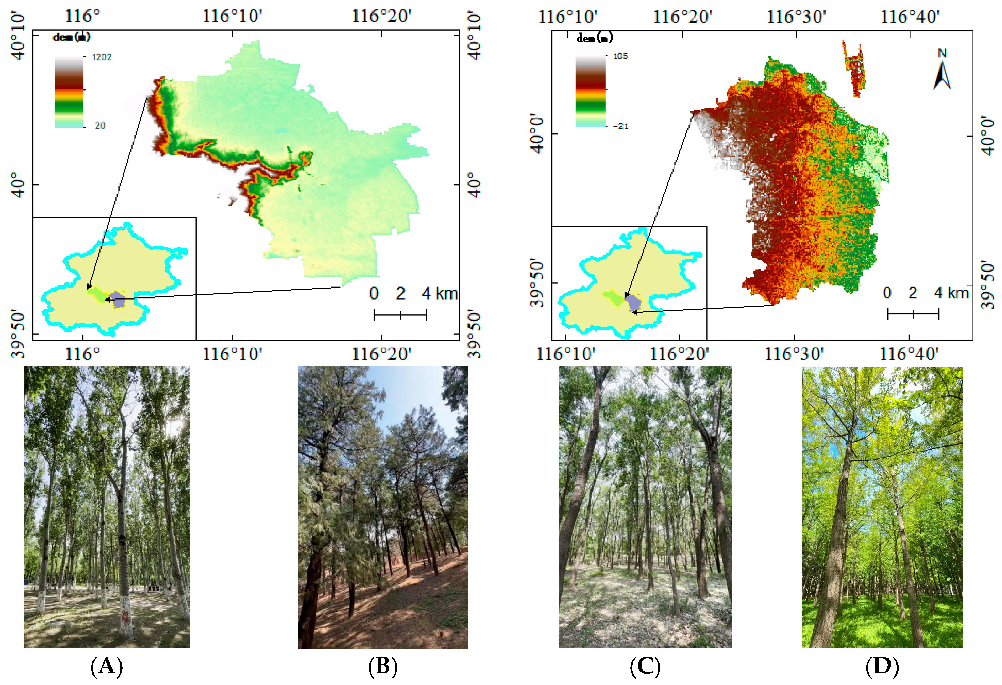
Figure 1. Overview of the study area. (A) Dongsheng Bajia Country Park—poplar; (B) Jiufeng—pine; (C) Olympic Forest Park—elm; (D) Olympic Forest Park—ginkgo.
Remotesensing 16 03845 g001
Figure 2. Comparison of camera position trajectories generated by Colmap. (A) Filming method with two circular paths. (B) Filming method with a single circular path around the forest plot.
Remotesensing 16 03845 g002
Figure 3. Technical framework.
Remotesensing 16 03845 g003
Figure 4. Comparison of sparse reconstruction point clouds under two filming methods. (A) Single circular path around the forest plot. (B) Two circular paths inside and outside the forest plot.
Remotesensing 16 03845 g004
Figure 5. Adaptive checkerboard propagation scheme of ACMMP. (Each V-shaped region contains 7 sampling pixels, and each strip region contains 11 sampling pixels. In the figure, Circles represent pixels. The black solid circle indicates the pixel to be estimated. The yellow circle represents the sampling point. During each propagation, the depth value of the red pixel is updated by the black pixel, and vice versa.).
Remotesensing 16 03845 g005
Figure 6. CDP-MVS dynamic domain propagation scheme (removing the central sample points and independently sampling in eight directions. Circles represent pixels. The black solid circle indicates the pixel to be estimated. During each propagation, the depth value of the red pixel is updated by the black pixel, and vice versa.).
Remotesensing 16 03845 g006
Figure 7. Reprojection flowchart. (The yellow line represents the process of projecting the pixel point p of the reference image to the point q in the adjacent image. The green line represents the process of re-projecting the point q back to the reference image.).
Remotesensing 16 03845 g007
Figure 8. Reference image (A) and its binarized grayscale image with sky segmentation (B).
Remotesensing 16 03845 g008
Figure 9. CDP-MVS algorithm flowchart.
Remotesensing 16 03845 g009
Figure 10. PatchMatchNet propagation sampling strategy. (Circles represent pixels. The black solid circle indicates the pixel to be estimated. During each propagation, the depth value of the red pixel is updated by the black pixel, and vice versa.).
Remotesensing 16 03845 g010
Figure 11. Dense point clouds reconstructed for three plots using different algorithms. (a) Poplar, (b) pine, (c) elm, (d) ginkgo. 1: CDP-MVS, 2: ACMMP, 3: PatchMatchNet.
Remotesensing 16 03845 g011aRemotesensing 16 03845 g011b
Figure 12. Comparison of canopy details reconstructed by different algorithms. (a) Poplar, (b) pine, (c) elm, (d) ginkgo. 1: CDP-MVS, 2: ACMMP, 3: PatchMatchNet.
Remotesensing 16 03845 g012aRemotesensing 16 03845 g012b
Figure 13. Comparison of trunk details reconstructed by different algorithms. (a) Poplar, (b) pine, (c) elm, (d) ginkgo. 1: CDP-MVS, 2: ACMMP, 3: PatchMatchNet.
Remotesensing 16 03845 g013aRemotesensing 16 03845 g013b
Figure 14. Scatter plot comparing reconstructed tree positions with actual positions (unit: meters). (a) Poplar, (b) pine, (c) elm, (d) ginkgo. 1: CDP-MVS, 2: ACMMP, 3: PatchMatchNet.
Remotesensing 16 03845 g014aRemotesensing 16 03845 g014b
Table 1. Plot information.
Sample PlotStand TypeRegionSlope (◦)Tree Count
APoplarDongsheng Bajia Park616
BPineJiufeng3624
CElmOlympic Forest Park1138
DGinkgoOlympic Forest Park2123
Table 2. Reconstruction time for three plots using different algorithms (unit: hours).
MethodPoplarPineElmGinkgo
CDP-MVS3.11.82.52.1
ACMMP3.21.82.682.23
PatchMatchNet8.356.436.036.57
Table 3. Accuracy of reconstructed tree quantity (unit: quantity).
Stand TypeMethodReconstructed Count Surveyed CountQAE
PoplarCDP-MVS1616100.00%
ACMMP1793.75%
PatchMatchNet1981.25%
PineCDP-MVS2424100.00%
ACMMP24100.00%
PatchMatchNet2595.83%
ElmCDP-MVS3838100.00%
ACMMP4192.11%
PatchMatchNet4484.21%
GinkgoCDP-MVS2323100.00%
ACMMP2591.30%
PatchMatchNet2686.97%
Table 4. Deviation between reconstructed and actual tree positions (index: AED, unit: meters).
MethodPoplarPineElmGinkgo
CDP-MVS0.140.250.190.13
ACMMP0.510.320.370.46
PatchMatchNet0.520.450.670.57
Table 5. Accuracy of reconstructed tree DBH (unit: centimeters).
Stand TypeMethodReconstructed Mean DBHMeasured Mean DBHAE
PoplarCDP-MVS22.1322.2396.27%
ACMMP22.0895.85%
PatchMatchNet23.1794.44%
PineCDP-MVS19.5220.6890.00%
ACMMP19.4389.76%
PatchMatchNet21.593.78%
ElmCDP-MVS21.319.6290.64%
ACMMP21.0788.55%
PatchMatchNet21.8290.09%
GinkgoCDP-MVS19.2720.3793.62%
ACMMP18.5890.25%
PatchMatchNet22.0589.27%
Table 6. Average relative error in tree height (unit: meters).
Stand TypeMethodReconstructed Mean HeightMeasured Mean HeightHAE
PoplarCDP-MVS17.8822.234.35
ACMMP18.074.16
PatchMatchNet17.674.56
PineCDP-MVS8.8911.052.16
ACMMP8.792.26
PatchMatchNet8.442.61
ElmCDP-MVS20.7626.315.55
ACMMP21.095.22
PatchMatchNet21.524.79
GinkgoCDP-MVS17.0721.654.58
ACMMP17.194.46
PatchMatchNet17.424.23
Disclaimer/Publisher’s Note: The statements, opinions and data contained in all publications are solely those of the individual author(s) and contributor(s) and not of MDPI and/or the editor(s). MDPI and/or the editor(s) disclaim responsibility for any injury to people or property resulting from any ideas, methods, instructions or products referred to in the content.