Abstract
The geographical location of Yunnan province is at the upstream area of water vapor transportation from the Bay of Bengal and the South China Sea to inland China. Understanding the spatiotemporal variations of water vapor over this region holds significant importance. We utilized the Global Navigation Satellite System (GNSS) data collected from 12 stations situated in Yunnan, which are part of the Crustal Movement Observation Network of China, to retrieve hourly precipitable water vapor (PWV) data from 2011 to 2022. The retrieved PWV data at Station KMIN were evaluated by the nearby radiosonde data, and the results show that the mean bias and RMS of the differences between the two datasets are 0.08 and 1.78 mm, respectively. Average PWV values at these stations are in the range of 11.77 to 33.53 mm, which decrease from the southwest to the north of Yunnan and are negatively correlated with the stations’ heights and latitudes. Differences between average PWV in the wet season and dry season range from 12 to 27 mm. These differences tend to increase as the average PWV increases. The yearly rates of PWV variations, averaging 0.18 mm/year, are all positive for the stations, indicating a year-by-year increase in water vapor. The amplitudes of the PWV annual cycles are 9.75–20.94 mm. The spatial variation of these amplitudes is similar to that of the average PWV over the region. Generally, monthly average PWV values increase from January to July and decrease from July to December, and the growth rate is less than the decline rate. Average diurnal PWV variations show unimodal PWV distributions over the course of the day at the stations except Station YNRL, where bimodal PWV distribution was observed.
1. Introduction
Water vapor in the atmosphere is a significant greenhouse gas [1,2] and it plays a crucial role in various atmospheric physical and chemical processes. Water vapor is the most active ingredient of the atmosphere. Its variations are closely associated with most weather phenomena. Additionally, water vapor exerts influence on the global water cycle and the heat balance between Earth and the atmosphere, as well as between the Earth–atmosphere system and outer space. It also facilitates the transport of heat from tropical regions to middle and high latitudes [3]. Thus, the observation of atmospheric water vapor content holds immense importance for weather, climate, and environment studies.
One term used to quantify the amount of water vapor is precipitable water vapor (PWV), which represents the depth of water in a column of the atmosphere if all the water in that column were precipitated as rain [4]. Atmospheric scientists have developed a variety of ways to measure PWV, but each has its limitations. Accurate PWV can be obtained by using radiosonde data, which include relative humidity, pressure, and temperature observations at different altitudes [5]. However, radiosondes are typically released only twice a day per site, and the distribution of these sites is relatively sparse. As a result, they cannot provide PWV data with high spatiotemporal resolution [6]. Ground-based water vapor radiometers are instruments that scan the sky and measure the microwave radiation emitted by atmospheric water vapor [7]. While they can provide PWV data with high temporal resolution, their spatial resolution is limited due to the limited number of these instruments in use. Satellite-based water vapor microwave radiometers can provide high-quality PWV data over oceans but face limitations over land. Although these microwave radiometers onboard low-earth-orbit satellites offer high spatial resolution, their temporal resolution is often compromised due to the long revisiting periods of the satellites. Infrared water vapor radiometers installed on geostationary satellites, e.g., Fengyun-4 satellites, retrieve PWV with high spatiotemporal resolutions (temporal resolution of 4–15 min and horizontal resolution of several kilometers) [8], but they are unable to accurately measure PWV on rainy or cloudy days.
Global Navigation Satellite System (GNSS) provides a cost-effective means of retrieving PWV with high temporal resolution, regardless of weather conditions [9]. The GNSS signals experience delays due to water vapor in the atmosphere. The relation between the zenith wet delay (ZWD) of the microwave signals and PWV was modeled by Askne and Nordius [10], establishing the basis for GNSS meteorology [11,12]. Since the usefulness of GNSS for water vapor retrieval was demonstrated [6,9], it has been widely used in meteorological and environmental studies. These include investigations into the relation between PWV and precipitation [13,14,15], deep convections [16,17,18], the effects of incorporating the GNSS-derived PWV into numerical weather prediction systems [19,20], summer monsoon and atmospheric rivers [21,22,23], and drought monitoring [24]. Moreover, the long-time and high temporal resolution GNSS-derived PWV data have been utilized to analyze secular trends and diurnal variations of PWV [25,26,27,28,29].
Yunnan province is situated in the southwestern region of China, bordering the southeastern side of the Tibetan Plateau. It occupies the headwater area of several major rivers, e.g., the Jinsha River and Nanpan River in Yunnan serve as the upper reaches of the Yangtze River and the Pearl River, respectively. Additionally, Yunnan is located in the upstream region of the water vapor transportation from the Bay of Bengal and the South China Sea to inland China. The variations in PWV across this area reflect changes in local weather patterns, climate conditions, and hydrological environment. Understanding these PWV variations is crucial for effective water resource and disaster management in Yunnan and downstream regions. Thus, many studies have focused on the PWV variations in this area. Fu et al. [30] and Hai et al. [31] utilized GPS data from 5–7 stations to analyze the PWV variations in Yunnan, but the PWV time series data used in their studies spanned only 1–3 years, which are insufficient for conducting secular PWV variation analyses. Shen and Duan [32] used the monthly NCEP/NCAR reanalysis data to examine the spatiotemporal variation of PWV in Yunnan, but the monthly data may not adequately capture short-term fluctuations, such as diurnal PWV variations. Li et al. [33] used GNSS data from 2010 to 2013 to analyze the multiscale temporal variations of PWV. Since their GNSS data were from a single station at Dali, their results and conclusions are confined to this small area rather than the entirety of Yunnan province. Hu et al. [34] investigated the variations of GNSS-derived PWV over the Yunnan-Guizhou Plateau. Their study focused on the relation between PWV and precipitation during convective weather in the summer season.
With the continuous advancements in both hardware and software of GNSS, the quality of GNSS observations has evidently improved. As the high-quality GNSS observations accumulate in Yunnan, it is of great importance to investigate PWV variations over this area with the recent GNSS observables and the latest data processing strategies. In this study, we adopted recent GNSS data over 11 years (2011–2022) from 12 stations located at Yunnan to derive hourly PWV data. First, we evaluated the GNSS-derived PWV data with radiosonde data. Then, we analyzed the geographical distributions of multiple-year-averaged PWV values across the region. Next, we determined and analyzed the secular trends and amplitudes of annual and semiannual cycles of PWV variations. At last, we investigated the monthly and diurnal variations of PWV at the individual stations. These analyses aim to provide a thorough understanding of the multiscale spatiotemporal variations of PWV and enhance our knowledge of the dynamic changes in PWV over Yunnan region.
2. Data and Methods
2.1. Data Description
The Crustal Movement Observation Network of China (CMONOC) has consistently conducted long-term observations of GNSS data, ensuring a reliable and high-quality dataset. In this study, we utilized GNSS data (sampling rate of 30 s) from CMONOC to retrieve hourly PWV data. The period of the used data extends from 1 July 2011 to 30 June 2022 (11 years). To ensure comprehensive coverage, we selected 12 stations located within Yunnan, spanning approximately 21°N to 29°N and 97°E to 107°E, to analyze PWV variations. The geographical distribution of the stations is shown in Figure 1 (red triangles). These stations are distributed with approximately even spacing. The longitudes, latitudes, and heights of the GNSS stations are shown in Table 1.
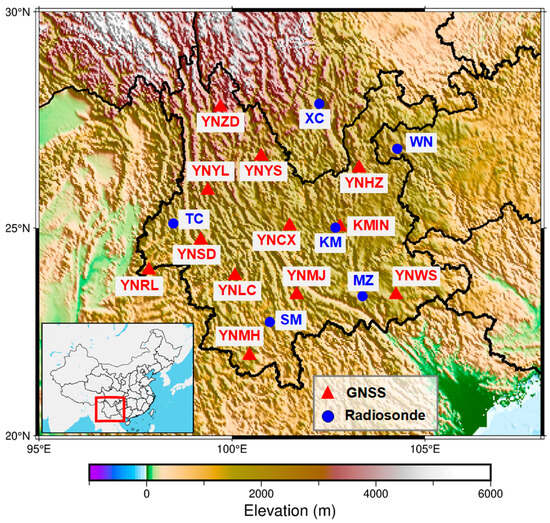
Figure 1.
Geographical distributions of GNSS and radiosonde stations. The red triangles mark the locations of the GNSS stations, and the blue dots denote the sites of radiosondes. The inset presents a zoomed-out map highlighting the province of Yunnan, enclosed by a distinct red rectangle.

Table 1.
The constructed Ts-Tm linear models and the coordinates of the related radiosonde sites and GNSS stations. The first column shows the coordinates and names of the radiosonde sites. Atmospheric profiles from these sites were utilized to construct Ts-Tm linear models shown in the second column. Each Ts-Tm linear model displayed on a row was used to calculate Tm for the GNSS stations presented on the same row, third column of the table.
Each GNSS station is equipped with a TRIMBLE NETR9 receiver that is connected to a TRM59800.00 or TRM59900.00 antenna. Additionally, there is a collocated meteorological sensor at each station to record air pressures and temperatures. The air pressures and temperatures are measured with accuracies of 0.3 mbar and 0.1 K, respectively. These measurements are essential for converting zenith tropospheric delay (ZTD) to PWV. During the conversion process, a key parameter is water vapor weighted mean temperature (Tm), which directly affects the accuracy of the converted PWV. Tm is usually estimated from the surface temperature (Ts) by using a simple linear model [9]. The linear relations between Ts and Tm are highly location dependent in the region of Yunnan [8,35,36], indicating that different Ts-Tm linear models may be adopted to calculate accurate Tm values at different GNSS stations. We used the atmospheric profile data (from 2005 to 2018) observed from 6 radiosonde stations to construct 6 site-specific Ts-Tm linear models, respectively. These radiosonde sites are within or near the region of Yunnan (blue dots in Figure 1). Table 1 shows the coordinates of the radiosonde stations, as well as their corresponding Ts-Tm linear models. Each constructed Ts-Tm linear model was utilized to calculate Tm for accurate PWV conversion at the nearby GNSS stations. The coordinates of these GNSS stations, along with their corresponding Ts-Tm linear models, are also shown in Table 1.
2.2. Retrieval of PWV
GNSS signals experience delays as they pass through the neutral atmosphere, resulting in the measured distances between satellites and receiving antennas to be longer than the actual distances. The slant path tropospheric delay (in length) can be calculated by
where SPD is the slant path delay in length, denotes the slant path passed by the GNSS signal, and is the refractive index of the atmosphere. The is not a constant and it varies based on several factors, including air pressures and temperature. Due to the challenges in obtaining accurate vertical profiles of in practice, Equation (1) is not commonly used to derive the SPD. In GNSS data processing, the tropospheric delay is estimated as an unknown quantity, and the ZTD instead of SPD is estimated to reduce the number of the unknowns. The relation between SPD and ZTD is
where MF is an elevation-angle-dependent mapping function. It can be written in continued fraction form as [37,38]
where is the elevation angle of site-to-satellite direction, and coefficients ,, and are derived from radiosonde data [39] or numerical weather models [38,40]. Equation (2) is suitable for the stations with azimuthal-symmetry local atmosphere. Under the circumstance of an unsymmetrical atmosphere, two gradient parameters are added into Equation (2) to compensate for the asymmetry [41].
The estimated ZTD can be partitioned into zenith hydrostatic delay (ZHD) and ZWD. By using the real observed surface air pressure, the ZHD can be modeled with an accuracy of several millimeters. The commonly used ZHD mode is [42]
where is the surface pressure (in mbar), is the latitude of the GNSS station, and is the height of the station (in meters). The ZWD can be acquired by ZTD minus ZHD. The conversion of ZWD to PWV is
where is a dimensionless coefficient, which is given by [9,43]
where is the density of liquid water (in Kg/m3); is the specific gas constant of water vapor (in J/(Kg·K)); ,, and are constants (in K/mbar) [9]; and are molar masses of water vapor and dry air, respectively (in g/mol); and Tm is the weighted mean temperature of atmosphere (in K). The definition of Tm is [44]
where is the partial pressure of water vapor (in mbar), and is the temperature (in K). The practical application of Equation (7) is limited because it relies on having accurate profiles of and , which are not readily available in many cases. Bevis et al. [9] used the radiosonde data to find the relation between Tm and surface temperature (Ts), and they fitted a linear Ts-Tm model. Thus, with this model, one can calculate the Tm from the observed surface temperature. We used a similar method to generate the Ts-Tm models specific for the study area (see Table 1 for the Ts-Tm models).
We used the Bernese GNSS software version 5.2 [45] to estimate ZTD. The data processing basically followed the default strategy of the Center for Orbit Determination in Europe (CODE) (Table 2).
Table 2.
Strategy of GNSS data processing.
The Bernese software always attempts to fix ambiguities to the maximum extent, but those ambiguities which do not satisfy the statistical threshold during ambiguity resolution are kept as floating-point numbers. In our data processing, on average, 70% of ambiguities were fixed as integers, the remaining were retained as floating-point values.
In this study, all the meteorological data used for converting GNSS ZTD to PWV (pressure for calculating ZHD and temperature for converting ZWD to PWV) are observed with the collocated meteorological equipment. We did not use other data (e.g., reanalysis data) or apply any interpolation to fill the gaps of the meteorological observations. Thus, the retrieved PWV time series are free of the potential biases caused by different meteorological data sources or by the interpolations.
3. Results
3.1. Continuity of GNSS ZTD and PWV Time Series
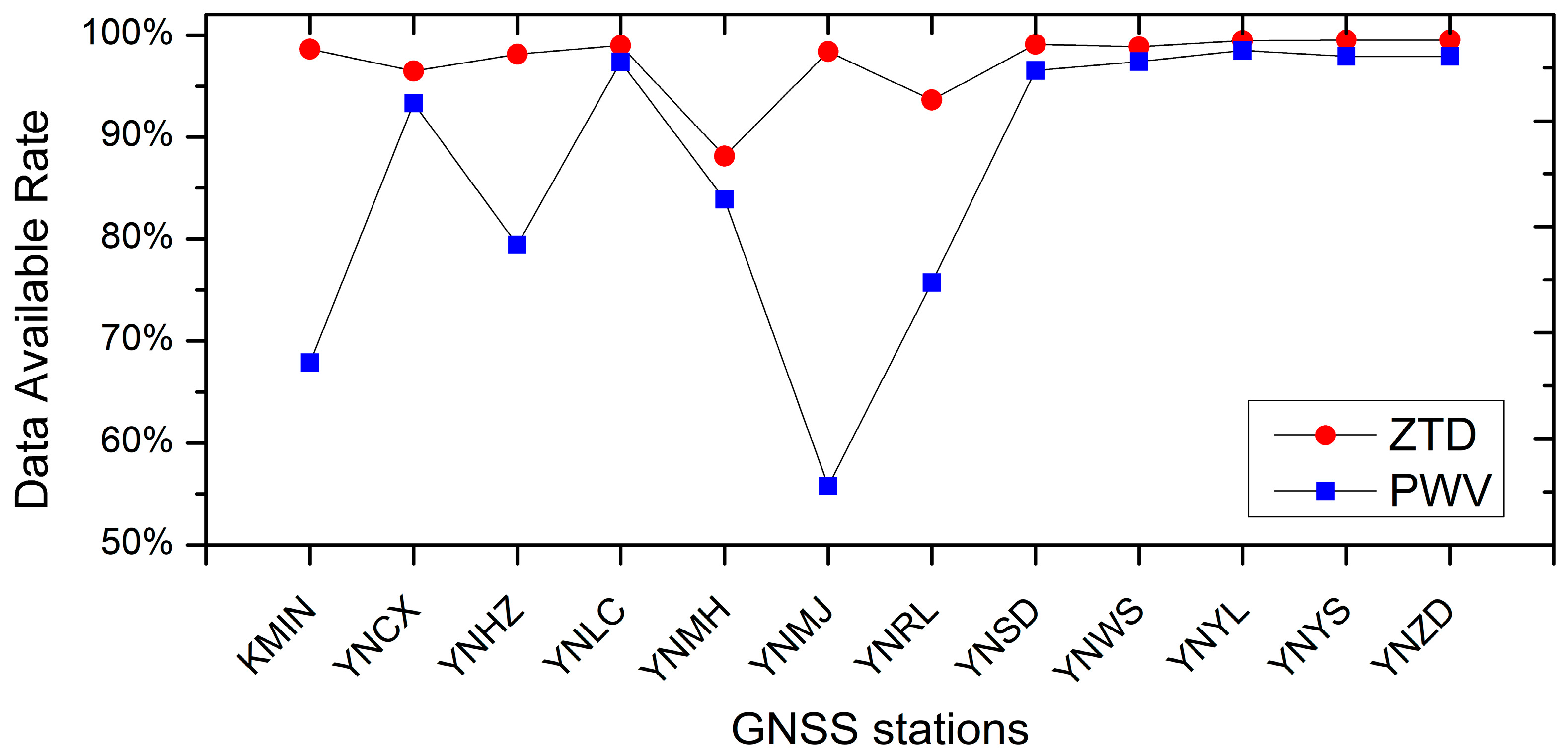
Using the 30 s-interval GNSS observations, we estimated ZTD on an hour-by-hour basis. Throughout the long-term observation period, the GNSS stations occasionally encounter some interruptions due to instrument and electrical failures. This causes the gaps in the observations. In addition, some noisy GNSS observations were eliminated in the phase of quality checking during data processing, which could further increase the gaps in the observations. As a result, ZTD on these corresponding epochs could not be estimated. For assessing the continuity of the derived ZTD and PWV time series, we set an evaluation index named Data Available Rate (DAR). The definition of DAR is the number of real retrieved data over the number of ideal continuous data. The DAR of ZTD for each station is shown in Figure 2 (red dots). The smallest DAR of ZTD is observed at Station YNMH, which is 88%. At the other 11 stations, DARs of ZTD are larger than 90%, with nine of them having a DAR greater than 98%. Regarding PWV, DAR values are comparable to those of ZTD at Stations YNCX, YNLC, YNMH, YNSD, YNWS, YNYL, YNYS, and YNZD. However, at the remaining stations, particularly at Station YNMJ, DARs of PWV are significantly lower than those of ZTD. These discrepancies arise due to a large number of missing meteorological observations at those stations and no interpolation being applied to fill the gaps of meteorological data for converting the corresponding ZTD into PWV.
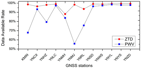
Figure 2.
Data available rates (DARs) of ZTD and PWV at each GNSS station. DAR = the number of real retrieved data/the number of ideal continuous data.
3.2. Evaluation of the GNSS PWV with Radiosonde Data
We evaluated GNSS-derived PWV with the radiosonde data. The GNSS station KMIN and radiosonde station Kunming are located in the same city, and the distance between them is less than 15 km. Thus, the two stations are well spatially matched. We retrieved the PWV from the radiosonde profiles (hereafter referred to as RDS-derived PWV). The PWV is calculated as
where is the specific humidity (in g/g), is the pressure of the atmosphere (in Pa), and is the gravitational acceleration (in m/s2). In the computation, is not regarded as a constant since its value is dependent on the latitude and height.
The temporal resolution of RDS-derived PWV is 12 h, while that of GNSS-derived PWV is 1 h. To ensure fair comparisons, we only chose data with the same epochs from the two datasets. This selection process resulted in a total of 4040 paired data points for the comparisons. Figure 3a shows both the time series of GNSS-derived PWV (red) and RDS-derived PWV (blue). The two datasets match each other very well. The average bias between them is 0.08 mm, and the RMS of the differences between them is 1.78 mm. There is a data gap of GNSS PWV with the period spanning from 2013 to 2015 at Station KMIN. An instrument failure at this station caused the missing of pressure and temperature observations. Without these meteorological observables, we were not able to convert the ZTD to PWV, which caused the data gap. Figure 3b shows the scatter points of the two datasets and also the linear fitting result. The slope of the linear fitted model is close to 1 (1.024) and the goodness of fit is 0.97, which all indicate that the two datasets are highly consistent. These comparisons demonstrate that the GNSS-derived PWV has similar accuracy to the RDS-derived one, and hence can be used for analyzing water vapor variations.
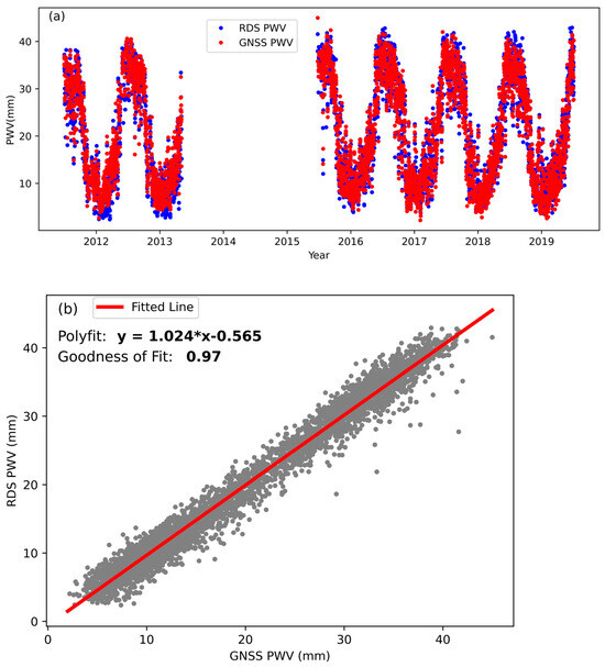
Figure 3.
Comparison of GNSS and radiosonde PWV at Station KMIN. (a) The time series of GNSS-PWV and RDS-PWV. (b) the goodness of fit between GNSS-PWV and RDS-PWV.
3.3. Average PWV and Spatial Distribution
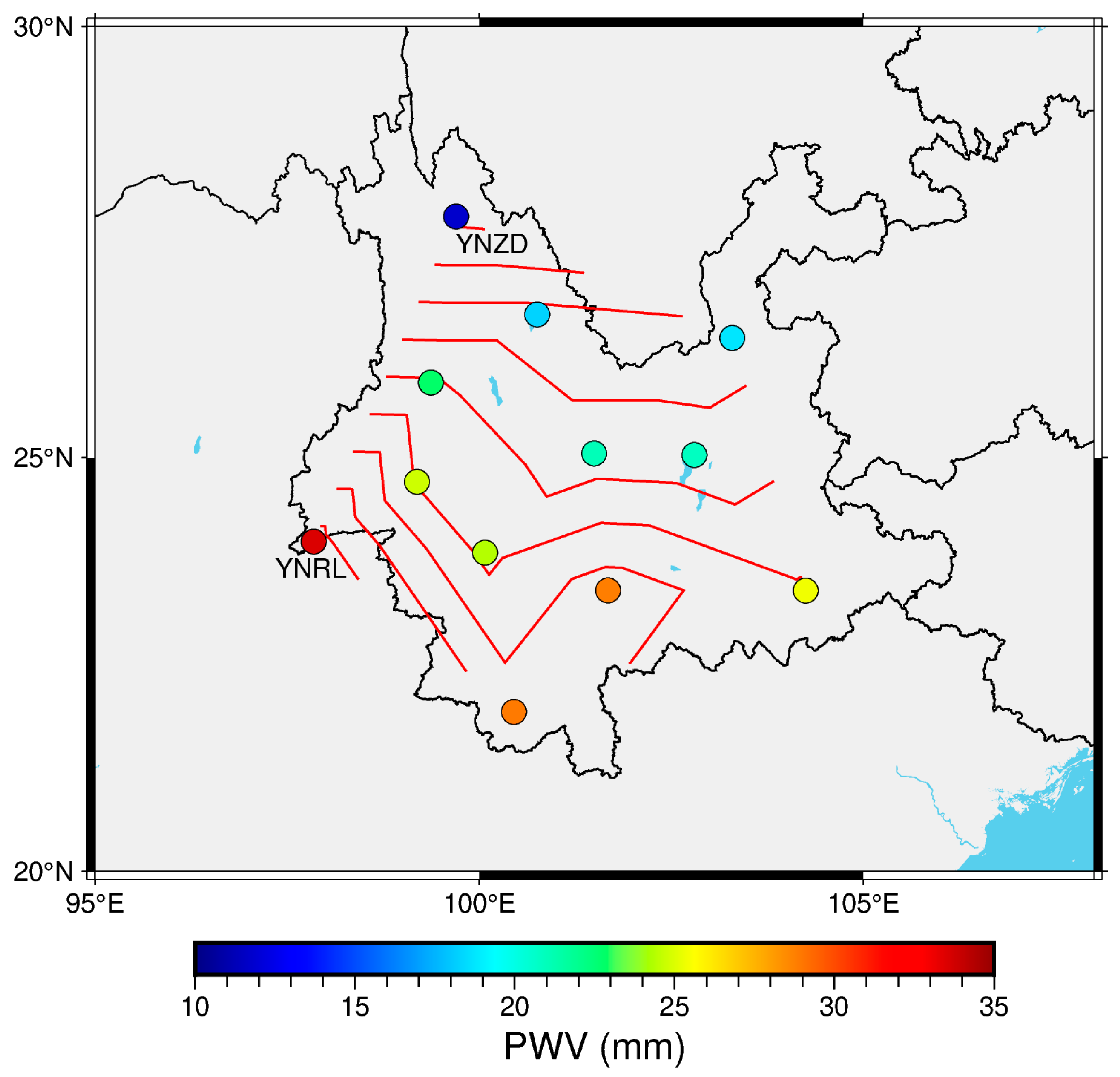
We averaged PWV values between 2011 and 2022 for each GNSS station. Figure 4 shows the geographical distribution of the average PWV. The largest average PWV is observed at Station YNRL located at the west boundary of Yunnan province, which is above 30 mm, while the smallest one is at Station YNZD located at the northwest of the area, which is only 11.8 mm (about 1/3 of the largest one). Average PWV values at the other stations are in the range of 18 to 29 mm. In general, the average PWV tends to decrease from southwest to the north of the area (Figure 4 contour lines). In addition to the all-season averaged PWV, we also calculated the average PWV in the wet season (June to October) and dry season (November to May) separately for the GNSS stations. The geographical distributions of wet-season and dry-season averaged PWV are similar to those of the all-season averaged PWV.
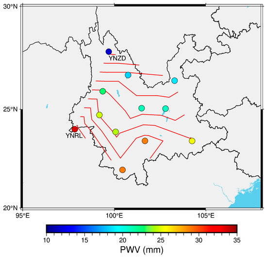
Figure 4.
Geographical distribution of 11-year-averaged PWV observed at the GNSS stations. The color on a circle indicates the value of average PWV at that station. The red lines are the contour lines of average PWV.
Figure 5 shows the relationship between the variation in average PWV and both the station height and latitude. The largest average PWV is observed at the station with the lowest height (YNRL: 723 m), while the smallest average PWV is at the highest station (YNZD: 3297). It clearly shows that the average PWV decreases as the height of the GNSS station increases. As for the latitudes, it shows that, in general, the average PWV decreases as the latitude of the station increases, except for Station YNRL. The latitude of Station YNRL is not the lowest one among the 12 GNSS stations; however, the average PWV observed at this station is the largest. This is probably subject to the special local climate of Station YNRL.
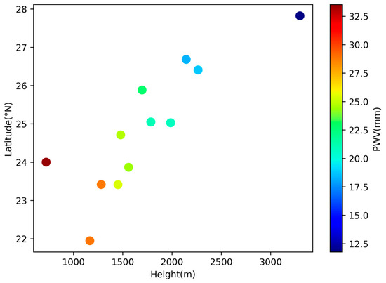
Figure 5.
Relation of the variation in average PWV with the station height and latitude. The color represents the value of average PWV.
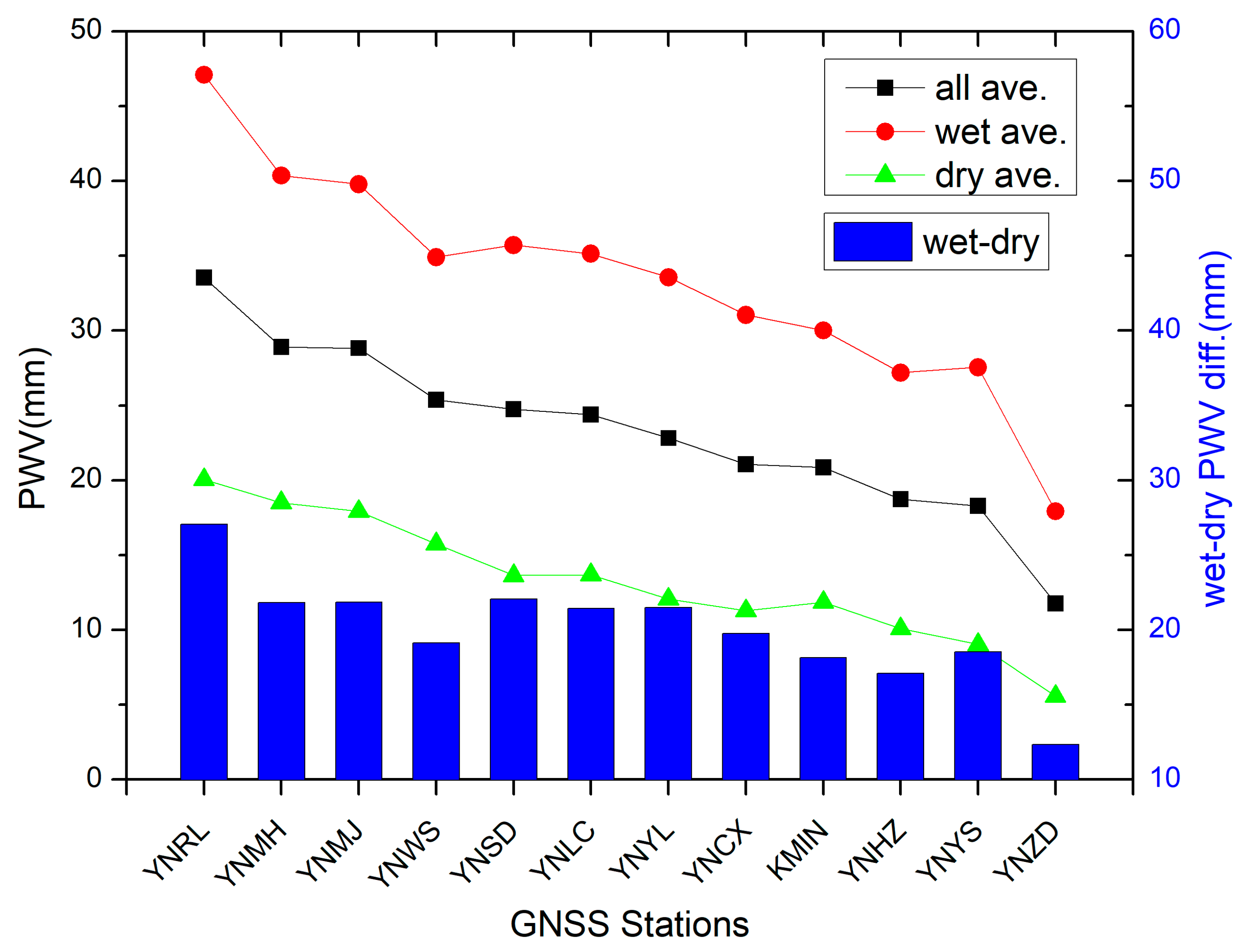
Figure 6 shows the all-season, wet-season, and dry-season averaged PWV for each station. At most stations, the average PWV values in the wet season are about 10 mm larger than those of the all-season averaged PWV, while the average PWV values in the dry season are smaller than those of the all-season averaged PWV by about 10 mm. The larger all-season averaged PWV values generally correspond to the larger average PWV values in both the wet season and dry season. The differences between average PWV in the wet season and dry season at these stations are in the range of 12 to 27 mm (Figure 6 blue bars). Overall, these differences tend to decease as the average PWV decreases.

Figure 6.
All-season (black), wet-season (red), and dry–season (green) averaged PWV for each GNSS station. A blue bar is the difference between the average PWV in wet season and dry season at the corresponding station. The stations are arranged in order of decreasing PWV.
3.4. Secular, Annual and Semiannual Variations of PWV
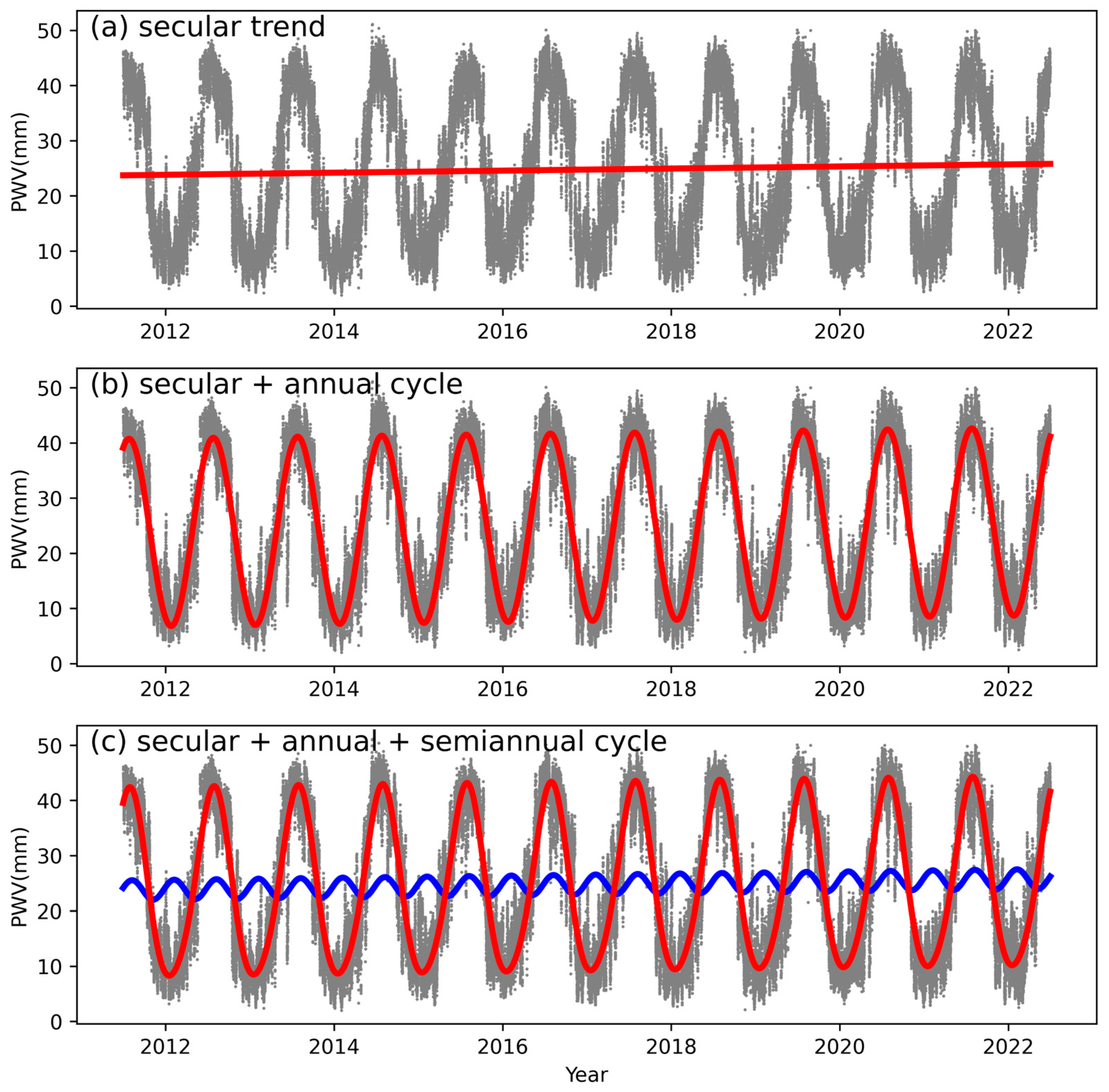
The time series of GNSS-derived PWV at these stations show significant annual cycles. Figure 7 shows the PWV variation at Station YNSD (other stations show similar variations). To quantitatively analyze the PWV time series at the stations, we modeled the PWV variations with a mathematical model that contains a secular trend, an annual cycle, and a semiannual cycle. The model is written as
where is the time in unit of year, and are the coefficients that describe the secular trend of PWV variation, and are the amplitudes of annual and semiannual PWV variations, and and are the initial phases.
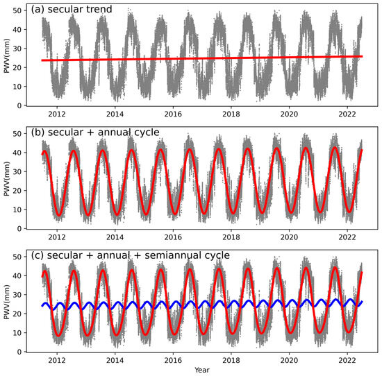
Figure 6.
GNSS-derived PWV time series at Station YNSD. The red solid line in (a) indicates the secular trend of PWV variations. The red sinusoid in (b) consists of the secular and the annual variation. In (c), the blue sinusoid is the semiannual variation superimposed on the secular trend, and the red sinusoid consists of the secular, annual, and semiannual variations.
We estimated the coefficients of Equation (9) by the least-squared method for each station. Figure 7a shows the secular trend of PWV variations at Station YNSD (red line). The secular trend is indistinctive, which indicates that the year-to-year change of PWV quantity is very slow. The superposition of the annual and secular variation for Station YNSD is shown in Figure 7b (red sinusoid), which well describes the magnitude of the fluctuation of PWV. When the term of semiannual variation (blue sinusoid in Figure 7c) is added, the model (red sinusoid in Figure 7c) fits the GNSS-derived PWV even better.
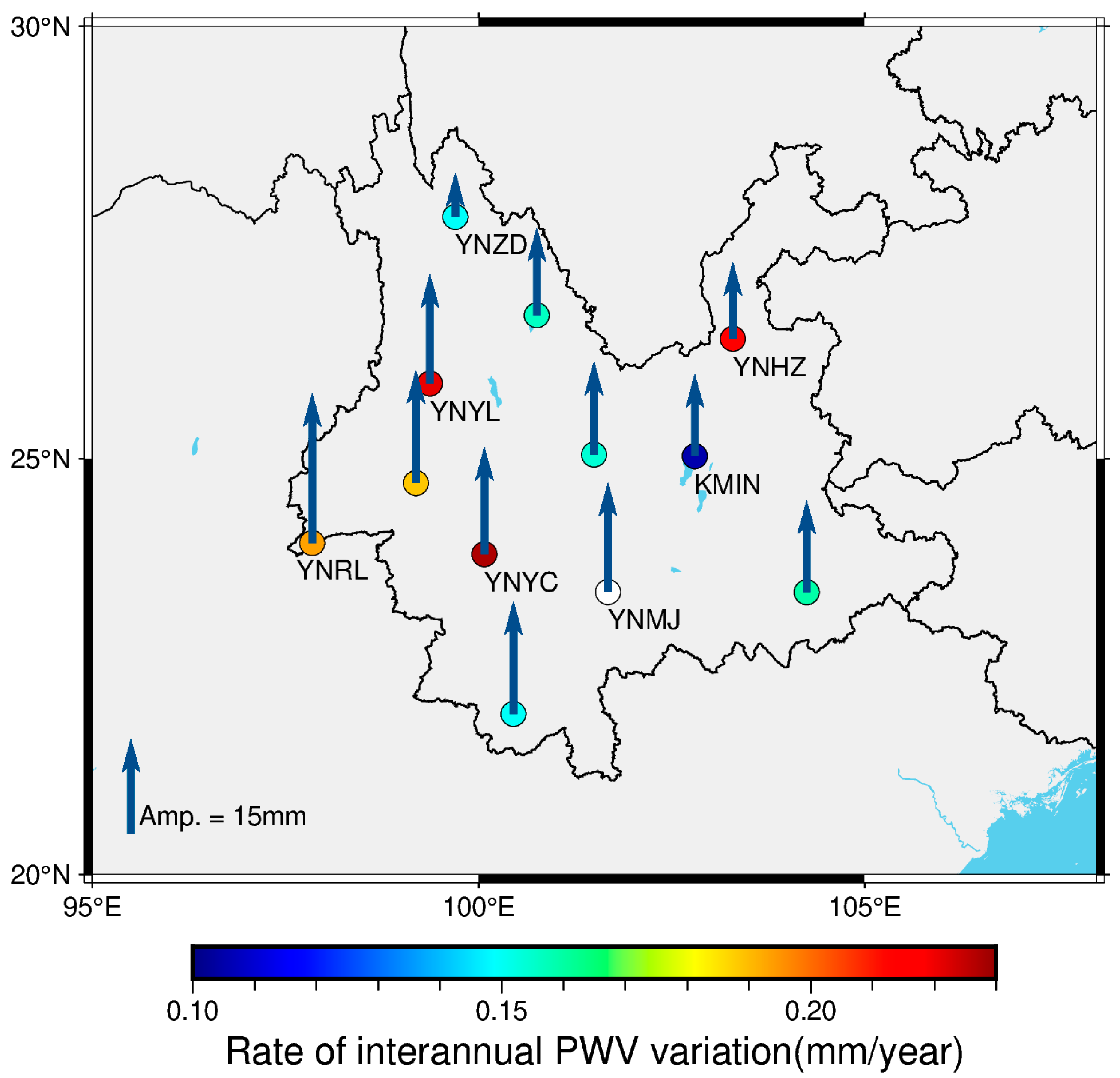
From the secular trends of PWV variations, we derived the rate of interannual PWV variations for each station. The rates are positive at all stations (Figure 8), averaging 0.18 mm/year, which indicates that the average PWV observed at each station increases yearly from 2011 to 2022. The minimal rate is observed at Station KMIN, which is 0.11 mm/year, while at Stations YNYC, YNYL, and YNHZ, the rates are up to or above 0.22 mm/year (twice the minimal rate). The derived rate of interannual PWV variations at Station YNMJ is 0.29 mm/year (not shown in Figure 8), which is significantly larger than the rates at the other stations. Due to the lack of collocated meteorological data before 2017 at Station YNMJ, the time span of the available GNSS-derived PWV data at this station (2017–2022) is much shorter than for the data from the other stations (2011–2022). Thus, we believe that the derived rate of interannual PWV variations at Station YNMJ is not as reliable as the derived rates at the other stations.
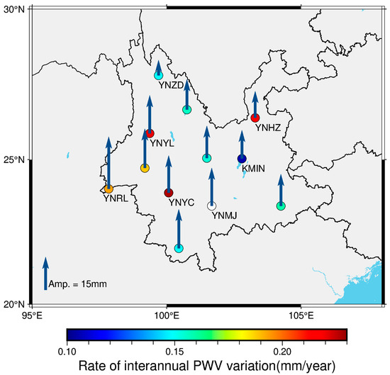
Figure 8.
Rate of interannual PWV variations and amplitude of annual PWV variations at each station. The colors filled in the circles indicate the rates of interannual PWV variations and the arrows denote the amplitudes of PWV annual variations.
Figure 8 also shows the amplitude of the annual cycle of PWV variations at each station. The average of the annual PWV variation amplitudes at these stations is 15 mm. The maximal amplitude is observed at Station YNRL, which reaches 20.9 mm, while the minimum is at Station YNZD, which is 9.7 mm. The distribution of the annual cycle amplitudes shows that the magnitude of the amplitude decreases from the southwest to the north of Yunnan region. This phenomenon is highly similar to the distribution of average PWV (refer to Figure 4 for the average PWV distribution), indicating that the larger average PWV values correspond to the greater amplitude of the annual cycle of PWV variations. The amplitudes of semiannual PWV variations, in the range of 0.3 to 2.5 mm, are much smaller than the annual amplitudes (compare the blue sinusoid in Figure 7c with red sinusoid in Figure 7b). On average, the semiannual amplitudes are about one tenth of the annual amplitudes.
3.5. Monthly and Diurnal Variations of PWV
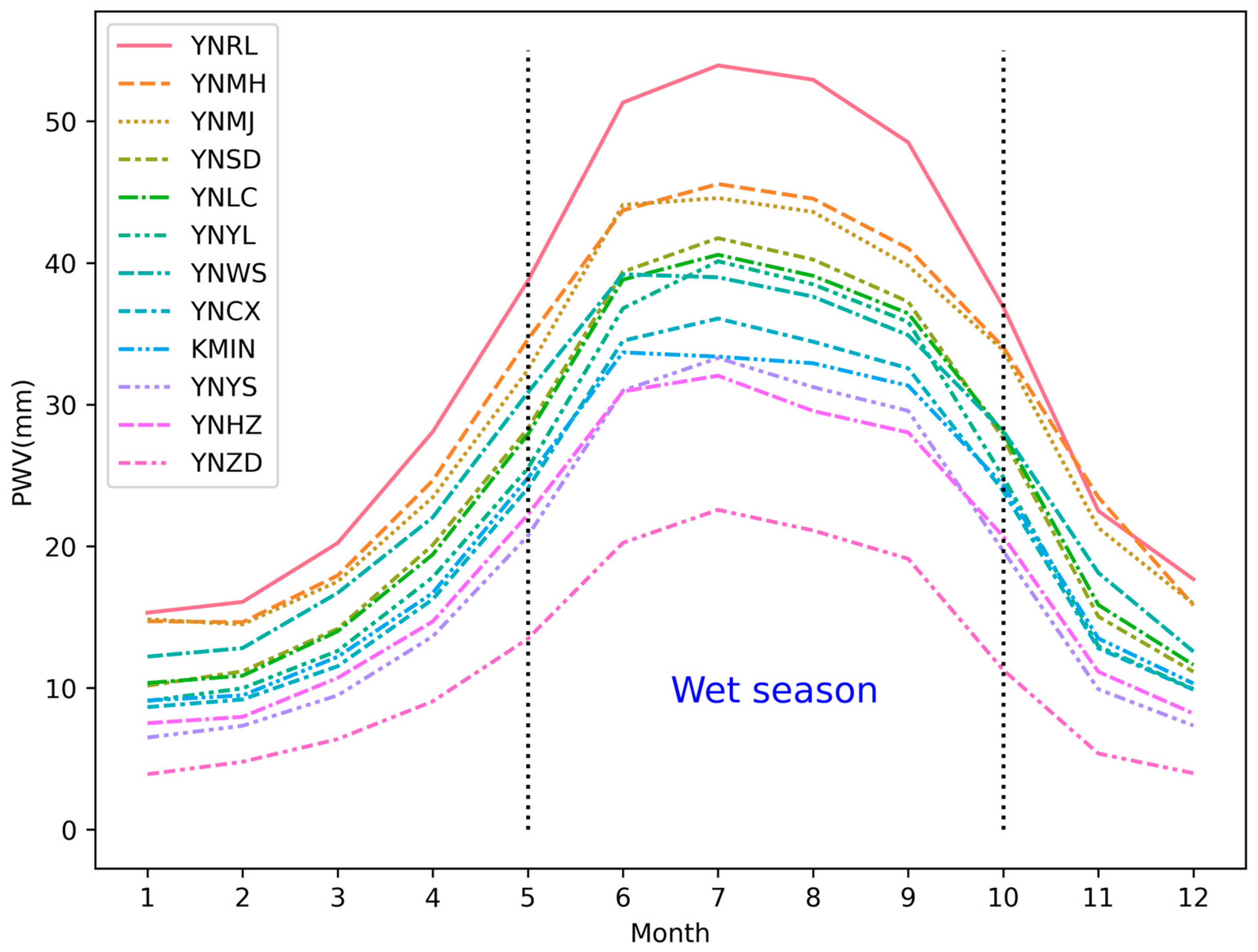
We averaged PWV values over the period from 2011 to 2022 for each individual month (January to December). Figure 9 shows the monthly variations in PWV at the 12 GNSS stations. The curves representing the month-to-month changes in PWV exhibit similar patterns across all stations. At most stations, the maximal monthly average PWV values are in July (Stations KMIN and YNWS in June), and the minimums are in January (Stations YNMH and YNMJ in February). The curves are not symmetric about the peaks: the increasing rates of PWV from January to July are less than the decreasing rates from July to December. The distribution of PWV is uneven among the seasons, with the wet season typically accounting for approximately 70% of the total PWV over the entire year on average.
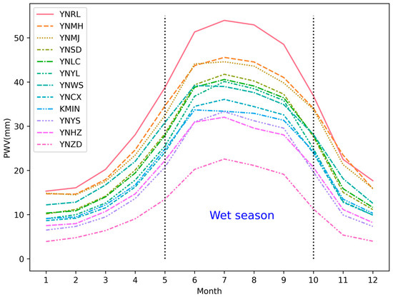
Figure 9.
Monthly PWV variation at each station.
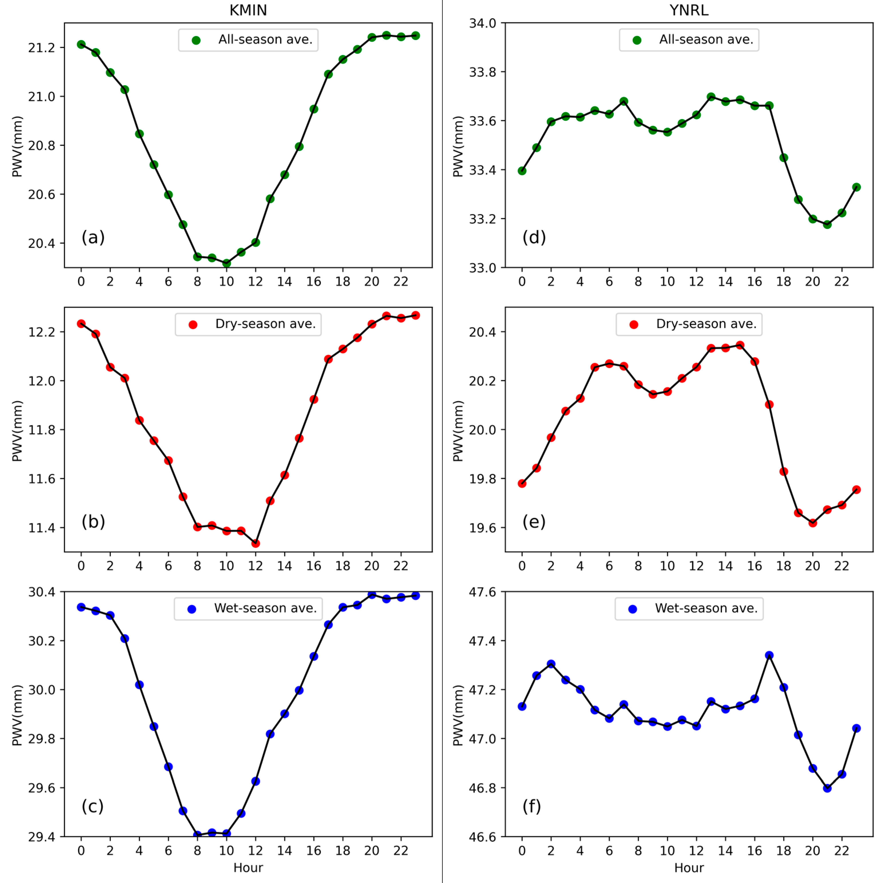
Using the hourly GNSS-derived PWV from 2011 to 2022, we calculated the all-season, wet-season, and dry-season average PWV values for each individual hour (0:00, 1:00, …, 23:00). Figure 10 shows the diurnal PWV variations at Stations KMIN and YNRL. The curves of all-season, wet-season, and dry-season averaged PWV diurnal variations are similar at the same station. Diurnal PWV variations at Station KMIN show the unimodal distribution pattern among the hours (Figure 10a–c). Data of the other stations show a similar pattern of PWV distribution as Station KMIN except for Station YNRL, where bimodal distribution of PWV is observed. At Station YNRL, the all-season, wet-season, and dry-season averaged diurnal variations of PWV all show that the high PWV values occur both in the afternoon and at night.
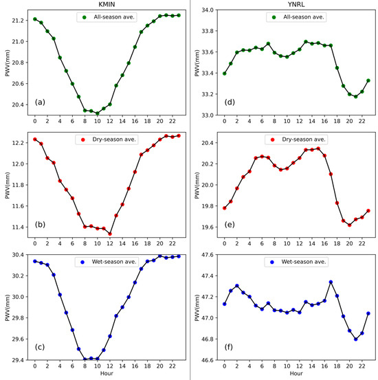
Figure 10.
Diurnal PWV variations at Stations KMIN (left) and YNRL (right): (a–c) are all-season, dry-season, and wet-season averaged diurnal PWV variations at Station KMIN, respectively, while (d–f) are for Station YNRL. The hours are local time.
Though diurnal PWV variations observed at 11 out of 12 GNSS stations show a similar unimodal distribution, the diurnal peaks (or valleys) of PWV values are asynchronous among different stations. Table 3 shows the time of diurnal peak and valley for the all-season, wet-season, and dry-season averaged PWV at each station (except Station YNRL). For these stations, the diurnal maximums (peaks) of the all-season averaged hourly PWV appear at 17:00–23:00 local time, most at 17:00–19:00 (late afternoon), while the diurnal minimums (valleys) occur at 8:00–10:00 (morning). The differences between the times of diurnal PWV peaks in the wet season and dry season are 0 to 5 h (most no more than 2 h). The times of diurnal PWV minimum in the dry season are 0 to 4 h later than those in the wet season (most no more than 1 h).
Table 3.
Hours (local time) of the diurnal PWV maximum (peak) and minimum (valley) at each station (except Station YNRL).
We calculated the magnitude of the diurnal PWV variation for each station. The magnitude, describing diurnal PWV fluctuation, is defined as the diurnal PWV peak minus valley. Figure 11 shows the geographical distribution of the magnitudes of diurnal PWV variations. The magnitudes of the diurnal PWV fluctuations, averaging 1.1 mm, are station dependent. The smallest magnitude (0.5 mm) is observed at Station YNRL, while at this station, both the average PWV and the amplitude of annual PWV variations are the largest among the other stations (refer to Figure 4 for the average PWV and Figure 8 for the amplitudes). The largest magnitude is at Station YNHZ (1.6 mm), which is about three times the magnitude at Station YNRL. However, Both the average PWV and the amplitude of annual PWV variations at Station YNHZ are much smaller than those at Station YNRL. The distribution of the magnitudes of diurnal PWV variations show no significant geographical pattern.
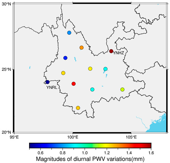
Figure 11.
Magnitude of diurnal PWV variation at each station. The magnitude is defined as the difference between the diurnal PWV maximum and minimum.
4. Discussion
We evaluated the GNSS-derived PWV with radiosonde data at Station KMIN, and the mean bias and RMS of the differences between the two datasets are 0.08 mm and 1.78 mm, respectively. Some previous studies also made similar comparisons in the region of Yunnan. Fu et al. [30] and Hai et al. [31] assessed the GNSS-derived PWV with RDS-derived PWV at 3–5 stations (including station KMIN) located at Yunnan. Their results show high correlations between the time series of GNSS-derived PWV and RDS-derived PWV (correlation coefficients larger than 0.9), which are consistent with our results. Nonetheless, their comparisons show 5–7 mm RMS of differences between the two datasets, which are much larger than the 1.78 mm RMS in this study. The results of Hai et al. [31] shows significant biases between the GNSS-derived PWV and RDS-derived PWV, while there are no evident biases observed in the current study and in the study of Fu et al. [30]. Hu et al. [34] used the ERA5 reanalysis dataset of the European Center for Medium-Range Weather Forecasts (ECMWF) to evaluate the GNSS-derived PWV, and their results show 2–6 mm biases and 4.5–7 mm RMS between GNSS-derived PWV and ERA5-derived PWV. There are many factors for the different evaluation results in these studies. Normally, the consistency of different-sourced PWV data in the wet season is poorer than that in the dry season. Hai et al. [31] and Hu et al. [34] exclusively used the summer data (in the wet season) for the evaluation, which is partly responsible for the large biases and RMS in their PWV assessments. We used the all-season data for the evaluation, and applied the latest mapping function to estimate the ZTD. Moreover, we generated the site-specific weighted mean temperature models for the region and used these customized models to convert the ZWD to PWV. All these contribute to the high consistency between GNSS-derived PWV and RDS-derived PWV in current study.
The distribution of all-season averaged PWV values show a clear southwest-to-north decreasing pattern in the region of Yunnan, and both the average PWV in wet season and dry season show a similar decreasing pattern. These results are consistent with the study of Shen and Duan [32]. In their study, the used PWV data were from a different source (NCEP/NCAR monthly reanalysis data), which further demonstrates the reliability of our derived PWV variation pattern. Their data are from 1981 to 2011, while ours are from 2011 to 2022, indicating that the PWV spatial variation pattern in Yunnan has not changed during the last four decades. Our results show that the content of PWV is highly dependent on the station height and latitude: a higher station height (or latitude) generally corresponds to less PWV. This negative correlation between PWV and station heights (or latitudes) was also found in the studies of Jin et al. [25] and Shi et al. [28]. These results are reasonable. The observed PWV is a quantity that integrated the water vapor from the station height to the top of the troposphere. It is inherently negatively correlated with the station height. Globally, high latitudes are colder than low latitudes. The ability of the atmosphere to hold water vapor decreases are the temperature decreases. These explain the negative correlation between the PWV value and the latitude.
The diurnal variations in PWV at the stations in Yunnan exhibit a predominantly unimodal distribution over the course of the day. However, it is worth noting that Station YNRL, located at the west boundary of Yunnan, displays a distinctive bimodal distribution of PWV. Hai et al. [31] found this bimodal diurnal PWV distribution at a different station in Mengla county, which is at the south boundary of Yunnan (see Figure A1 in Appendix A). These bimodal diurnal PWV distributions were observed at both the west (Station YNRL at Ruili county) and south (Mengla county) boundary of Yunnan, indicating the special local climate at these border areas.
5. Conclusions
Using GNSS data observed at 12 CMONOC stations located at Yunnan, China, we retrieved the hourly PWV from 2011 to 2022 and analyzed multiscale spatiotemporal PWV variations over the region. Evaluating the GNSS-derived PWV with radiosonde data at Station KMIN shows good consistency between the two datasets, indicating that the GNSS-derived PWV is as accurate as RDS-derived PWV and hence it can be reliably used in meteorological studies. In the study area, the average PWV values observed at different stations can be quite different: the maximum is three times as large as the minimum. Generally, the average PWV increases with the decrease in station height, and also with the decrease in station latitude (excluding Station YNRL). For these stations, the higher average PWV in the wet season corresponding to higher average PWV in the dry season, and the mean of the differences between average PWV in the wet season and dry season is 20 mm. We analyzed the secular trends and cycles of the PWV time series. The yearly rates of PWV variations are all positive at the 12 stations. This phenomenon of increasing PWV year by year is in line with the context of climate warming. The average amplitude of PWV annual cycles is 15 mm, which is about 10 times as large as the average amplitude of PWV semiannual cycles. Monthly PWV variations show that the maximal monthly average PWV occurs in July or June, and the minimum appears in January or February. The content of average PWV in the wet season accounts for 70% of the sum of PWV over the entire year. Average diurnal PWV variations show unimodal distributions over the course of the day at the stations, while Station YNRL is an exception, where two diurnal PWV peaks were observed. At most stations, the average diurnal PWV maximums occur in the late afternoon (17:00–19:00), and the minimums appear in the morning (8:00–10:00).
In this study, both the largest average PWV and the greatest amplitude of the annual PWV cycle were observed at Station YNRL. The diurnal PWV distribution of this station (bimodal) is different from that of the other stations (unimodal). Furthermore, the average PWV at this station did not follow the rule of negative correlation between PWV and latitude as the other stations do. All these indications suggest that the local climate at Station YNRL differs from that of the other stations, which deserves further investigation.
Author Contributions
Conceptualization, M.W.; methodology, M.W., Z.L., D.L., and W.W.; software, W.W. and Z.L.; Validation R.Z. and C.S.; formal analysis, M.W. and C.S.; data curation, W.W. and R.Z.; writing—original draft preparation, M.W.; writing—review and editing, W.W. All authors have read and agreed to the published version of the manuscript.
Funding
This research was funded by the National Natural Science Foundation of China (NO. 42374022; 42304008), the Opening Project of Shanghai Key Laboratory of Space Navigation and Positioning Techniques (NO. 202103), the Research Program of China Seismic Experimental Site (NO. CEAIEF20220403), the Open Fund of Key Laboratory of Marine Environmental Survey Technology and Application, Ministry of Natural Resources (NO. MESTA-2020-B011), the Guangdong Basic and Applied Basic Research Foundation (NO. 2019A1515011268), and the Guangzhou Science and Technology Plan Project (NO. 202102020380).
Data Availability Statement
The radiosonde data used in this study are available from http://weather.uwyo.edu/upperair/sounding.html (accessed on 1 January 2023). The generated ZTD and PWV data are available from the corresponding author on reasonable request.
Acknowledgments
The authors are grateful to the Crustal Movement Observation Network of China (CMONC) for providing the GNSS data and the collocated meteorological observables, and they would like to thank three anonymous reviewers for their constructive comments and useful suggestions to improve the manuscript.
Conflicts of Interest
The authors declare no conflict of interest.
Appendix A

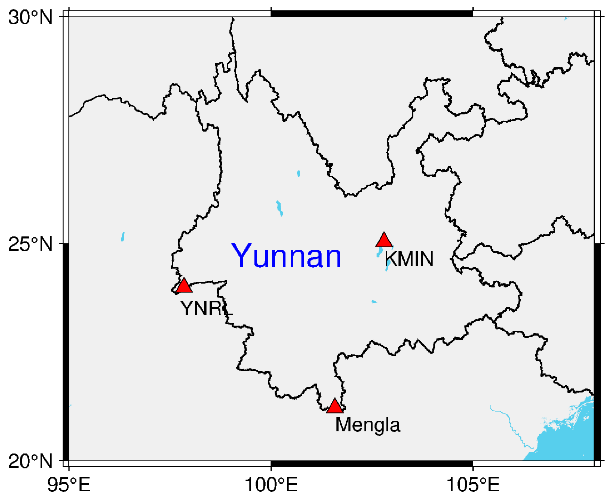
Figure A1.
Locations of Station Mengla, Station YNRL, and Station KMIN. The red triangles mark the locations of the GNSS stations.
Figure A1.
Locations of Station Mengla, Station YNRL, and Station KMIN. The red triangles mark the locations of the GNSS stations.
References
- Anand, K.; Inamdar, V.; Ramanathan, N.; Loeb, G. Satellite observations of the water vapor greenhouse effect and column longwave cooling rates: Relative roles of the continuum and vibration-rotation to pure rotation bands. J. Geophys. Res.-Atmos. 2004, 109, 1–9. [Google Scholar]
- Easterbrook, D. Greenhouse gases. In Evidence-Based Climate Science: Data Opposing CO2 Emissions as the Primary Source of Global Warming, 2nd ed.; Easterbrook, D., Ed.; Elsevier: Oxford, UK, 2016; pp. 163–173. [Google Scholar]
- Mills, E. Weather Studies: Introduction to Atmospheric Science, 6th ed.; American Meteorological Society: Boston, MA, USA, 2015. [Google Scholar]
- Salby, M. Fundamentals of Atmospheric Physics; Academic Press: San Diego, CA, USA, 1996; pp. 25–29. [Google Scholar]
- Wang, J.; Zhang, L.; Dai, A.; Immler, F.; Sommer, M.; Vomel, H. Radiation dry bias correction of Vaisala RS92 humidity data and its impacts on historical radiosonde data. J. Atmos. Ocean. Technol. 2013, 30, 197–214. [Google Scholar] [CrossRef]
- Rocken, C.; Ware, R.; Van Hove, T.; Solheim, F.; Alber, C.; Johnson, J.; Bevis, M.; Businger, S. Sensing atmospheric water vapor with the Global Positioning System. Geophy. Res. Lett. 1993, 20, 2631–2634. [Google Scholar] [CrossRef]
- Rocken, C.; Hove, T.; Johnson, J.; Solheim, F.; Ware, R.; Bevis, M.; Chiswell, S.; Businger, S. GPS/STORM—GPS sensing of atmospheric water vapor for meteorology. J. Atmos. Ocean Tech. 1995, 12, 468–478. [Google Scholar] [CrossRef]
- Wang, M. The Assessment and Meteorological Applications of High Spatiotemporal Resolution GPS ZTD/PW Derived by Precise Point Positioning. Ph.D. Thesis, Tong University, Shanghai, China, 2019. [Google Scholar]
- Bevis, M.; Businger, S.; Herring, T.; Rocken, C.; Anthes, R.; Ware, R. GPS meteorology: Remote sensing of atmospheric water vapor using the Global Positioning System. J. Geophys. Res. 1992, 97, 15787–15801. [Google Scholar] [CrossRef]
- Askne, J.; Nordius, H. Estimation of tropospheric delay for microwaves from surface weather data. Radio Sci. 1987, 22, 379–386. [Google Scholar] [CrossRef]
- Duan, J.; Bevis, M.; Fang, P.; Bock, Y.; Chiswell, S.; Businger, S.; Rochen, C.; Solheim, F.; Van Hove, T.; Ware, R.; et al. GPS meteorology: Direct estimation of the absolute value of precipitable water. J. Appl. Meteorol. 1996, 35, 830–838. [Google Scholar] [CrossRef]
- Fang, P.; Bevis, M.; Bock, Y.; Gutman, S.; Wolfe, D. GPS meteorology: Reducing systematic errors in geodetic estimates for zenith delay. Geophys. Res. Lett. 1998, 25, 3583–3586. [Google Scholar] [CrossRef]
- Cao, Y.; Fang, Z.; Xia, Q. Relationship between GPS precipitable water vapor and precipitation. J. Appl. Meteorol. Sci. 2005, 16, 54–59. [Google Scholar]
- Van Baelen, J.; Reverdy, M.; Tridon, F.; Labbouz, L.; Dick, G.; Bender, M.; Hagen, M. On the relationship between water vapour field evolution and the life cycle of precipitation systems. Q. J. R. Meteorol. Soc. 2011, 137, 204–223. [Google Scholar] [CrossRef]
- Huang, L.; Mo, Z.; Xie, S.; Liu, L.; Chen, J.; Kang, C.; Wang, S. Spatiotemporal characteristics of GNSS-derived precipitable water vapor during heavy rainfall events in Guilin, China. Satell. Navig. 2021, 2, 13. [Google Scholar] [CrossRef]
- Brenot, H.; Neméghaire, J.; Delobbe, L.; Clerbaux, N.; De Meutter, P.; Deckmyn, A.; Deckmyn, A.; Deleloo, A.; Frappez, L.; Roozendael, M. Preliminary signs of the initiation of deep convection by GNSS. Atmos. Chem. Phys. 2013, 13, 5425–5449. [Google Scholar] [CrossRef]
- Adams, D.; Barbosa, H.; Gaitán De Los Ríos, K. A spatiotemporal water vapor-deep convection correlation metric derived from the Amazon dense GNSS meteorological network. Mon. Weather Rev. 2017, 145, 279–288. [Google Scholar] [CrossRef]
- Shi, C.; Zhou, L.; Fan, L.; Zhang, W.; Cao, Y.; Wang, C.; Xiao, F.; Lv, G.; Liang, H. Analysis of ‘21·7’ extreme rainstorm process in Henan Province using BeiDou/GNSS observation. Chin. J. Geophys.-CH 2022, 65, 186–196. [Google Scholar]
- Vedel, H.; Huang, X. Impact of ground based GPS data on numerical weather prediction. J. Meteorol. Soc. JPN 2004, 82, 459–472. [Google Scholar] [CrossRef]
- Bennitt, G.; Jupp, A. Operational assimilation of GPS zenith total delay observations into the Met Office numerical weather prediction models. Mon. Weather Rev. 2012, 140, 2706–2719. [Google Scholar] [CrossRef]
- Means, J. GPS precipitable water as a diagnostic of the north American monsoon in California and Nevada. J. Clim. 2013, 26, 1432–1444. [Google Scholar] [CrossRef]
- Moore, A.; Small, I.; Gutman, S.; Bock, Y.; Dumas, J.; Fang, P.; Haase, J.; Jackson, M.; Laber, J. National weather service forecasters use GPS precipitable water vapor for enhanced situational awareness during the Southern California Summer Monsoon. Bull. Am. Meteorol. Soc. 2015, 96, 1867–1877. [Google Scholar] [CrossRef]
- Wang, M.; Wang, J.; Bock, Y.; Liang, H.; Dong, D.; Fang, P. Dynamic mapping of the movement of landfalling atmospheric rivers over southern California with GPS data. Geophys. Res. Lett. 2019, 46, 3551–3559. [Google Scholar] [CrossRef]
- Zhao, Q.; Ma, X.; Yao, W.; Liu, Y.; Yao, Y. A drought monitoring method based on precipitable water vapor and precipitation. J. Clim. 2020, 33, 10727–10741. [Google Scholar] [CrossRef]
- Jin, S.; Li, Z.; Cho, J. Integrated water vapor field and multiscale variations over China from GPS measurements. J. Appl. Meteorol. Clim. 2008, 47, 3008–3015. [Google Scholar] [CrossRef]
- Jin, S.; Luo, O. Variability and climatology of PWV from global 13-year GPS observations. IEEE Trans. Geosci. Remote 2009, 47, 1918–1924. [Google Scholar] [CrossRef]
- Wang, J.; Zhang, L. Climate applications of a global 2-hourly atmospheric precipitable water dataset derived from IGS tropospheric products. J. Geod. 2009, 83, 209–217. [Google Scholar] [CrossRef]
- Shi, C.; Zhang, W.; Cao, Y.; Lou, Y.; Liang, H.; Fan, L.; Satirapod, C.; Trakolkul, C. Atmospheric water vapor climatological characteristics over Indo-China region based on BeiDou/GNSS and relationships with precipitation. Acta Geod. Cartogr. Sin. 2020, 49, 1112–1119. [Google Scholar]
- Wu, M.; Jin, S.; Li, Z.; Cao, Y.; Ping, F.; Tang, X. High-precision GNSS PWV and its variation characteristics in China based on individual station meteorological data. Remote Sens. 2021, 13, 1296. [Google Scholar] [CrossRef]
- Fu, R.; Duan, X.; Liu, J.; Sun, J.; Wang, M.; Chen, X.; Liu, Y. Characteristics of ground-based GPS-retrieved PWV in Yunnan. Meteorol. Sci. Technol. 2010, 38, 456–462. [Google Scholar]
- Hai, Y.; Sun, J.; Chen, X. The analysis of GPS-retrieved PWV characteristic in Yunnan from 2007–2010. Yunnan Geogr. Environ. Res. 2011, 23, 78–84. [Google Scholar]
- Shen, Y.; Duan, W. Characteristics of temporal and spatial distribution of water vapor resource in Yunnan area. Environ. Sci. Surv. 2016, 35, 36–41. [Google Scholar]
- Li, Y.; Xu, A.; Dong, B. Variation characteristics of precipitable water volume observed by GPS in Dali. J. Meteorol. Res. Appl. 2020, 41, 32–37. [Google Scholar]
- Hu, H.; Cao, Y.; Shi, C.; Lei, Y.; Wen, H.; Liang, H.; Tu, M.; Wan, X.; Wang, H.; Liang, J.; et al. Analysis of the precipitable water vapor observation in Yunnan–Guizhou Plateau during the convective weather system in summer. Atmosphere 2021, 12, 1085. [Google Scholar] [CrossRef]
- Wang, M.; Cao, Y.; Liang, H.; Tu, M.; Liu, Z. On the accuracy of regional weighted mean temperature linear models over China. J. Nanjing Univ. Inf. Sci. Technol. (Nat. Sci. Ed.) 2021, 13, 161–169. [Google Scholar]
- Wang, M.; Chen, J.; Han, J.; Zhang, Y.; Fan, M.; Yu, M.; Sun, C.; Xie, T. Region-specific and weather-dependent characteristics of the relation between GNSS weighted mean temperature and surface temperature over China. Remote Sens. 2023, 15, 1538. [Google Scholar] [CrossRef]
- Niell, A. Preliminary evaluation of atmospheric mapping functions based on numerical weather models. Phys. Chem. Earth 2001, 26, 475–480. [Google Scholar] [CrossRef]
- Böhm, J.; Schuh, H. Vienna mapping functions in VLBI analyses. Geophy. Res. Lett. 2004, 31, L01603. [Google Scholar] [CrossRef]
- Neill, A. Global mapping functions for the atmosphere delay at radio wavelengths. J. Geophys. Res. 1996, 101, 3227–3246. [Google Scholar] [CrossRef]
- Böhm, J.; Niell, A.; Tregoning, P.; Schuh, H. Global mapping function (GMF): A new empirical mapping function based on data from numerical weather model data. Geophys. Res. Lett. 2006, 33, L07304. [Google Scholar] [CrossRef]
- Davis, J.; Elgered, G.; Niell, A.; Kuehn, C. Ground based measurement of gradients in the “wet” radio refractivity of air. Radio Sci. 1993, 28, 1003–1018. [Google Scholar] [CrossRef]
- Saastamoinen, J. Atmospheric correction for troposphere and stratosphere in radio ranging of satellites. In The Use of Artificial Satellites for Geodesy; Henriksen, S., Mancini, A., Chovitz, B., Eds.; William Byrd Press: Richmond, VA, USA, 1972; Volume 15, pp. 247–252. [Google Scholar]
- Bevis, M.; Businger, S.; Chiswell, S.; Herring, T.; Anthes, R.; Rocken, C.; Ware, R. GPS meteorology: Mapping zenith wet delays onto precipitable water. J. Appl. Meteorol. 1994, 33, 379–386. [Google Scholar] [CrossRef]
- Davis, J.; Herring, T.; Shapiro, I.; Rogers, A.; Elgered, G. Geodesy by radio interferometry: Effects of atmospheric modeling errors on estimates of baseline length. Radio Sci. 1985, 20, 1593–1607. [Google Scholar] [CrossRef]
- Dach, R.; Lutz, S.; Walser, P.; Fridez, P. Bernese GNSS Software Version 5.2; User Manual; Astronomical Institute, University of Bern, Bern Open Publishing: Bern, Switzerland, 2015; ISBN 978-3-906813-05-9. [Google Scholar] [CrossRef]
- Chen, G.; Herring, T. Effects of atmospheric azimuthal asymmetry on the analysis of space geodetic data. J. Geophy. Res. 1997, 102, 20489–20502. [Google Scholar] [CrossRef]


Disclaimer/Publisher’s Note: The statements, opinions and data contained in all publications are solely those of the individual author(s) and contributor(s) and not of MDPI and/or the editor(s). MDPI and/or the editor(s) disclaim responsibility for any injury to people or property resulting from any ideas, methods, instructions or products referred to in the content. |
© 2024 by the authors. Licensee MDPI, Basel, Switzerland. This article is an open access article distributed under the terms and conditions of the Creative Commons Attribution (CC BY) license (https://creativecommons.org/licenses/by/4.0/).