Abstract
The Yangtze River Basin (YZRB) and the Yellow River Basin (YRB), which are crucial for ecology and economy in China, face growing challenges to ecosystem service (ES) functions due to global population growth, urbanization, and climate change. This study assessed the spatiotemporal dynamics of ESs in the YZRB and the YRB between 2001 and 2021, comprehensively encompassing essential aspects such as water yield (WY), carbon sequestration (CS), soil conservation (SC), and habitat quality (HQ) while also analyzing the trade-offs and synergies among these ESs at the grid cells. The GeoDetector was employed to ascertain individual or interactive effects of natural and anthropogenic factors on these ESs and their trade-offs/synergies. The results showed that (1) from 2001 to 2021, the four ESs exhibited significant spatial disparities in the distribution within two basins, with the overall trend of ESs mainly increasing. YZRB consistently exhibited substantially higher ES values than the YRB. (2) Complex trade-offs and synergies among these ESs were apparent in both basins, characterized by distinct spatial heterogeneity. The spatial relationships of WY–CS, WY–SC, CS–SC, and CS–HQ were mainly synergistic. (3) Precipitation, potential evapotranspiration, elevation, land use and land cover (LULC), and slope influenced ESs in both basins. Notably, interactive factors, particularly the interactions involving LULC and other factors, demonstrated more robust explanatory power for ESs and their trade-offs/synergies than individual drivers. These findings significantly affect the refined ecosystem management and sustainable development decision-making in large rivers or regions.
1. Introduction
Ecosystems are the Earth’s support systems, playing key roles in the preservation of biodiversity, the provisioning of resources, climate regulation, the maintenance of soil health, pollution mitigation, habitat preservation, cultural enrichment, and the facilitation of sustainable development [1,2,3]. Ecosystem services (ESs), as derivations and benefits accrued directly or indirectly from the structure, processes, and functions of ecosystems by humanity [4,5], principally encompass provisioning, supporting, regulating, and cultural services [6]. However, with the increase in global population, the expansion of urbanization, and the threat of climate change to ecosystems, the supply capacity and quality of ESs are facing severe challenges (such as water scarcity, reduced food production, habitat loss, etc.) [7,8]. Moreover, anthropogenic activities marked by the overexploitation of natural resources perpetually disrupt the structural and functional aspects of ecosystems, leading to a range of ecological challenges, such as atmospheric pollution, water contamination, soil erosion, climate warming, land degradation, and biodiversity decline [9,10,11]. To address these challenges, researchers of geography, ecology, economics, and other disciplines have particularly focused on the diverse relationships among ESs and the impact of multiple factors on them, considering ESs key research priorities [12,13]. Therefore, a comprehensive and in-depth study of ES driving mechanisms, relationships, and conservation measures has become imperative.
The quantification of ESs is crucial in understanding the contributions of natural ecosystems to the societal system and is a primary task in achieving regional sustainability. Presently, ES assessments have transitioned from static evaluations (single points in time) to dynamic analyses (multi-scale) of ecological processes, with an augmented emphasis on the impact of ESs on human well-being [5,6,14]. The assessment methods predominantly employed include the value-based and the material-based approach. The former employs methodologies rooted in mathematics and economics to directly or indirectly assess ESs in monetary terms [5,15]. However, the quantification of the monetary value of ESs is a complex process with significant disparities in evaluation methodologies [16,17,18]. Conversely, the material-based approach encompasses the energy-based method and biophysical modeling, which offers a comprehensive quantitative evaluation of various ESs from a material perspective [19,20]. The energy-based method may encounter challenges in practical implementation due to difficulties in data acquisition. In contrast, biophysical modeling can provide a robust spatial representation of ESs and reveal the fundamental mechanisms behind their provision.
With the development of remote sensing and geographic information technologies, biophysical modeling methods based on multi-parameters, which provide dynamic spatial support for the assessment of ESs [8], have been realized. Currently, ES assessment models based on biophysical modeling mainly include Artificial Intelligence for ESs [21], Land Utilization and Capability Indicator [22], Spatial Evaluation for the Natural Capital Evidence [23], Social Values for the ESs [24], Toolkit for ES Site-based Assessments [25], and Integrated Valuation of ESs and Tradeoffs (InVEST) [26]. Each model with unique functionalities, varying simulation accuracy, and decision support should be selected comprehensively based on specific objectives, data availability, and regional requirements [27]. The InVEST model integrates ecological production functions, economic evaluation techniques, and versatile features like dynamic modeling, spatial analysis, multi-scale adaptability, modularity, and scenario assessment. It has been widely applied in diverse disciplines worldwide, including ecology, geography, and hydrology [28,29]. Although some studies have indicated that the Soil & Water Assessment Tool (SWAT) was accurate or reliable, the results obtained from the SWAT and InVEST models showed significant correlations [30,31]. Decsi et al. [32] argued that InVEST is the most efficient hydrological ES tool considering computational demand, result reliability, and data and expertise requirements. Moreover, one of its notable features is that all its modules are independent, allowing users to customize data according to their research needs. This has demonstrated effectiveness in assessing ESs such as water yield, water quality purification, soil retention, carbon storage, and biodiversity conservation [33,34,35].
However, the various ESs, environmental heterogeneity, and human preferences lead to interrelations characterized by trade-offs or synergies among these services [8,36]. Trade-offs involve consuming one ES to enhance another, while synergies refer to situations where two ESs increase or decrease simultaneously [36,37]. The trade-offs and synergies cannot be directly quantified but are analyzed through changes in ES quantities as an intermediary approach [38]. Statistical, spatial, and scenario analyses are common methods for studying trade-offs and synergies [39,40]. Scenario analysis, however, requires further improvement in terms of theoretical development and validation [40]. Statistical methods like correlation coefficients can effectively reveal the mechanisms of relationships between ESs and provide an intuitive analysis of the results but often focus on the overall difference of coefficients [41]. However, different regions have different environmental characteristics, and different areas and social groups have different demands and dependencies on ESs, resulting in heterogeneity of the spatial distribution of ES relationships [42,43]. Understanding the spatial heterogeneity of the trade-offs and synergies between ESs is essential for achieving a refined ecosystem management [44]. Then, correlation analysis based on grid cells combines spatial analysis methods and better represents the spatial relationships among ESs regarding trade-offs and synergies [37,45]. Furthermore, the trade-offs and synergies among ESs depend on the spatiotemporal scale [46]. However, previous studies on ESs at spatial scales were conducted at global, national, regional, and watershed scales, whereas ignoring the ESs relationships at the grid cells may affect these at large scales [46,47]. Time scales were selected based on a single year or discrete time series (years with a specific time interval) [12,46]. Although Local Indicators of Spatial Association (LISA) can identify spatial relationships between ESs [48], they are often used to analyze ESs in single or dual periods. Nevertheless, the relationships between ES systems are not static trade-offs or synergies but can change due to external factors such as natural variations, climate change, and human activities [8,49]. Focusing only on ESs for discrete years may overlook the impact of continuous trade-offs and synergies, thereby affecting the accuracy of the analysis results [50]. Therefore, it is necessary to investigate the relationships between ESs and their driving mechanisms of continuous long-time series at the grid cells, which can provide decision-makers with more specific and targeted information, formulating more effective environmental management and resource utilization strategies.
The Intergovernmental Science-Policy Platform on Biodiversity and Ecosystem Service (IPBES) [51] assessment of natural factors and human activities influencing changes in ecosystem functions and structures highlighted climate change as a primary driving factor in any ecosystem domain, including terrestrial and freshwater ecosystems. Climate change impacts the supply of ESs by altering ecosystem structures and functions. Global warming is predicted to increase extreme weather events, such as heavy rainfall and extreme heat, posing threats to ESs related to climate regulation, nutrient cycling, soil formation, and photosynthesis [12,52]. Land-use change, a result of human activities, directly modifies ecosystem structures and functions by altering land types for development and utilization [53]. Additionally, human activities such as population growth and urbanization expansion increase the demand for ESs, leading to changes in the functionality of food provision, habitat protection, soil conservation, and biodiversity [12]. Among various methods for analyzing drivers, traditional methods like principal component analysis and regression analysis face challenges in handling the spatial variability of driving factors. Geographically weighted regression model (GWR) and GeoDetector are the most commonly used methods for exploring the driving mechanism of ecosystem spatial heterogeneity. Most of the studies that have used the GWR model to investigate the factors affecting the spatial heterogeneity of variables have been statistical analyses of the correlations between variables and their effects, having lacked direct quantitative explorations of the relationships and ignoring the interactions between the factors [54]. GeoDetector, a spatial analysis method, adeptly identifies spatial variations and uncovers causal drivers, enabling the assessment of individual spatial variances and the interrelation of spatial patterns between two variables, thus facilitating the exploration of potential causal links between them [45,55]. It has been widely used to analyze the drivers of ESs, urban expansion, population distribution, vegetation change, extreme events, etc. [54,56,57].
The Yangtze River Basin (YZRB) and the Yellow River Basin (YRB) are China’s two most important rivers; they are paramount to socio-economic development. Despite its abundant natural resources, diverse economic and cultural activities, and significant geographical advantages, the YZRB faces challenges from intensive human activities, complex human-environment interactions, ecological fragility, and frequent droughts and floods [58]. The YRB encompasses several vital ecological functional zones, such as Three River Headwaters, Qilian Mountain, Qinling Mountain, etc. Still, it grapples with a poor ecological foundation, severe water scarcity, significant soil erosion, weak resource and environmental carrying capacity, and particularly prominent issues of imbalanced and insufficient development across its provinces and regions along the river [12,59]. Therefore, the YZRB and the YRB were selected as the study areas, and meteorological data, soil data, and multi-source remote sensing data were utilized as data sources, model simulations, statistical methods, and GIS spatial mapping techniques, which were employed to achieve the following specific objectives: (1) to explore the spatiotemporal trends in multiple ESs in the YZRB and the YRB from 2001 to 2021, (2) to analyze the trade-offs and synergies among these ESs at the grid cells of continuous time series, and (3) to reveal the influence of natural and human factors on each ES and the associated trade-offs and synergies. The findings not only provide policy recommendations for regional economic development and sustainable resource management in the YZRB and the YRB but also serve as a significant case study and profound insight for global efforts in managing large rivers, understanding the impacts of climate change, preserving biodiversity, and achieving sustainable development goals.
2. Materials and Methods
2.1. Study Area
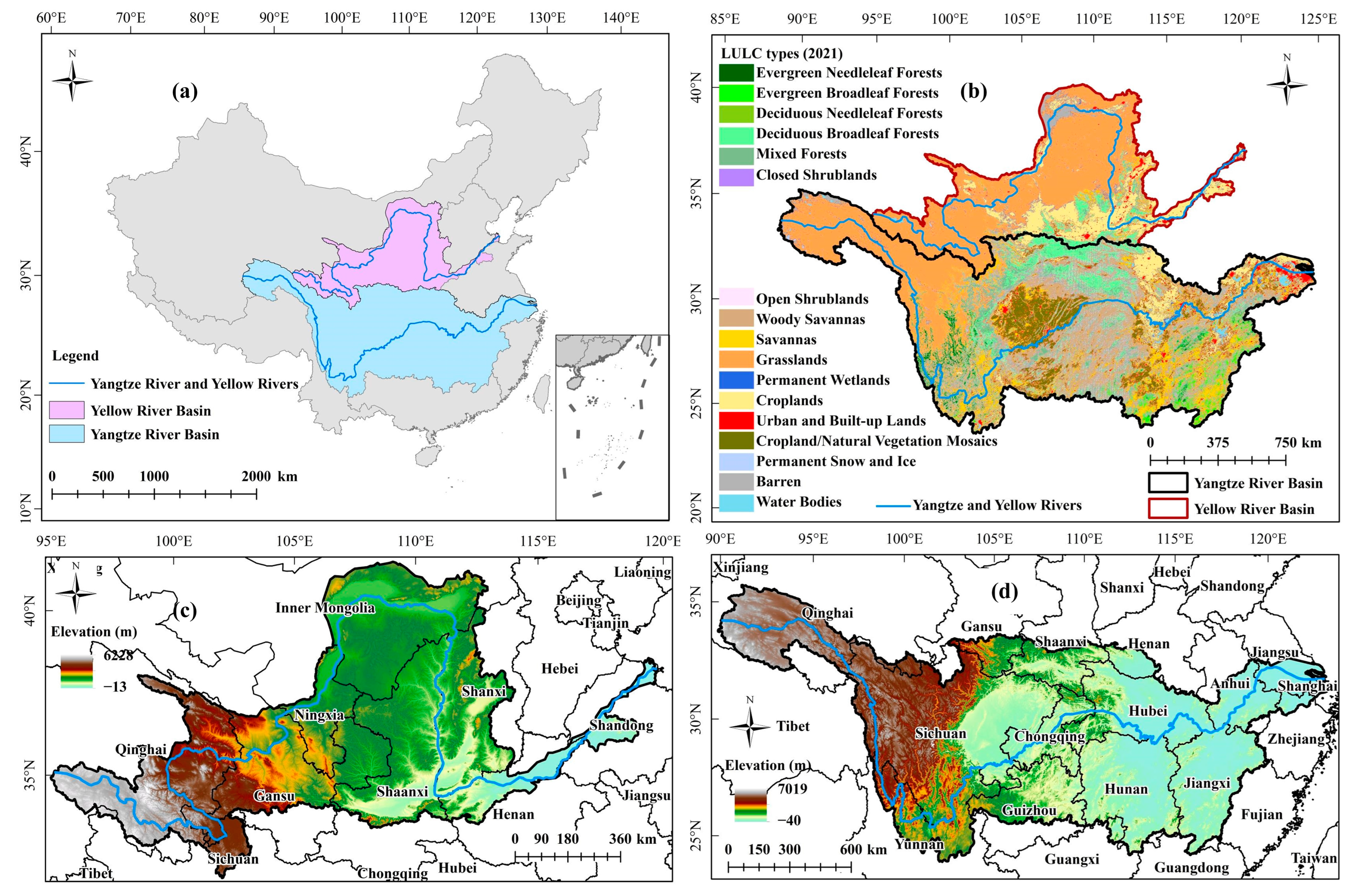
The Yangtze and Yellow Rivers, originating from the Qinghai–Tibet Plateau, have obvious differences in geographical environments, climatic characteristics, and water resources (Figure 1). The YZRB (24°30′–35°45′N, 90°33′–122°33′E) spans a total length of 6397 km, covering a total area of 1.8 million km2. The topography is three steps down from west to east: (1) the first step includes the Southern Qinghai Plateau, the Western Sichuan Plateau, and the Hengduan Mountains, with an elevation of 3500–5000 m; (2) the second step is composed of the Qinba Mountains, Sichuan Basin, Yunnan–Guizhou Plateau, and Hubei–Guizhou Mountains, with an elevation of 500–2000 m; and (3) the third step is the Huaiyang Mountains, Jiangnan Hills, and the Middle and Lower Reaches of the Yangtze River Plain, which are generally below 500 m above sea level. The geomorphological types are diverse and complex, with mountain areas covering about 80% (https://www.resdc.cn/, accessed on 1 June 2023). The climate is dominated by subtropical monsoons, which are characterized as being hot and humid in summer and cold and dry in winter. The average annual precipitation and temperature are about 1064 mm and 9.1 °C, respectively (https://www.nmic.cn/, accessed on 1 October 2022). The YRB (32°10′–41°50′N, 95°53′–119°05′E) flows a total length of 5464 km, covering a total of 795,000 km2. The terrain is distributed from west to east in lowered steps, with mountain areas accounting for about 70% (https://www.resdc.cn/, accessed on 1 June 2023). The YRB experiences a continental climate characterized by significant differences in precipitation and temperature, with the average precipitation and temperature of the whole basin over the past 20 years being 460.5 mm and 2.4 °C, respectively (https://www.nmic.cn/, accessed on 1 October 2022).
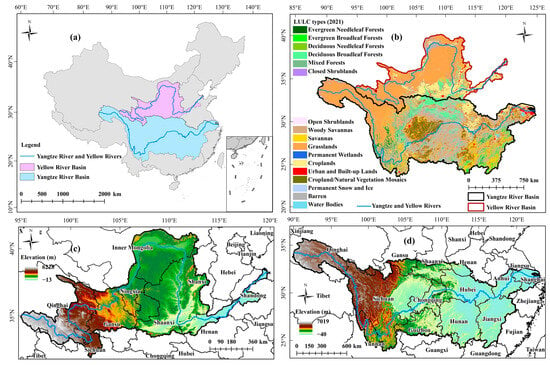
Figure 1.
Study area: (a) geographical location of two study areas; (b) LULC types; (c,d) elevation distributions.
The two basins also exhibit significant differences in human activities, such as land use and land cover (LULC), gross domestic product (GDP), and population density (POD) [12]. The YZRB features a diverse and complex land cover, primarily grassland, forestland, and cultivated land (Figure 1b). Regions with intense population activities, such as urban areas, are mainly distributed along the Yangtze River, forming continuous urban agglomerations with a relatively higher level of economic development [60]. In contrast, the YRB is predominantly grassland, with fewer forests (shrubland types) (Figure 1b). Urban areas in the YRB occupy less areas and are not obviously distributed along the Yellow River due to spatial and natural resource limitations, resulting in relatively lower POD and economic development [61]. These differences require a focus on sustainable economic development in the YZRB and point out the importance of ecological conservation and long-term environmentally friendly development in the YRB [12].
2.2. Data Source and Processing
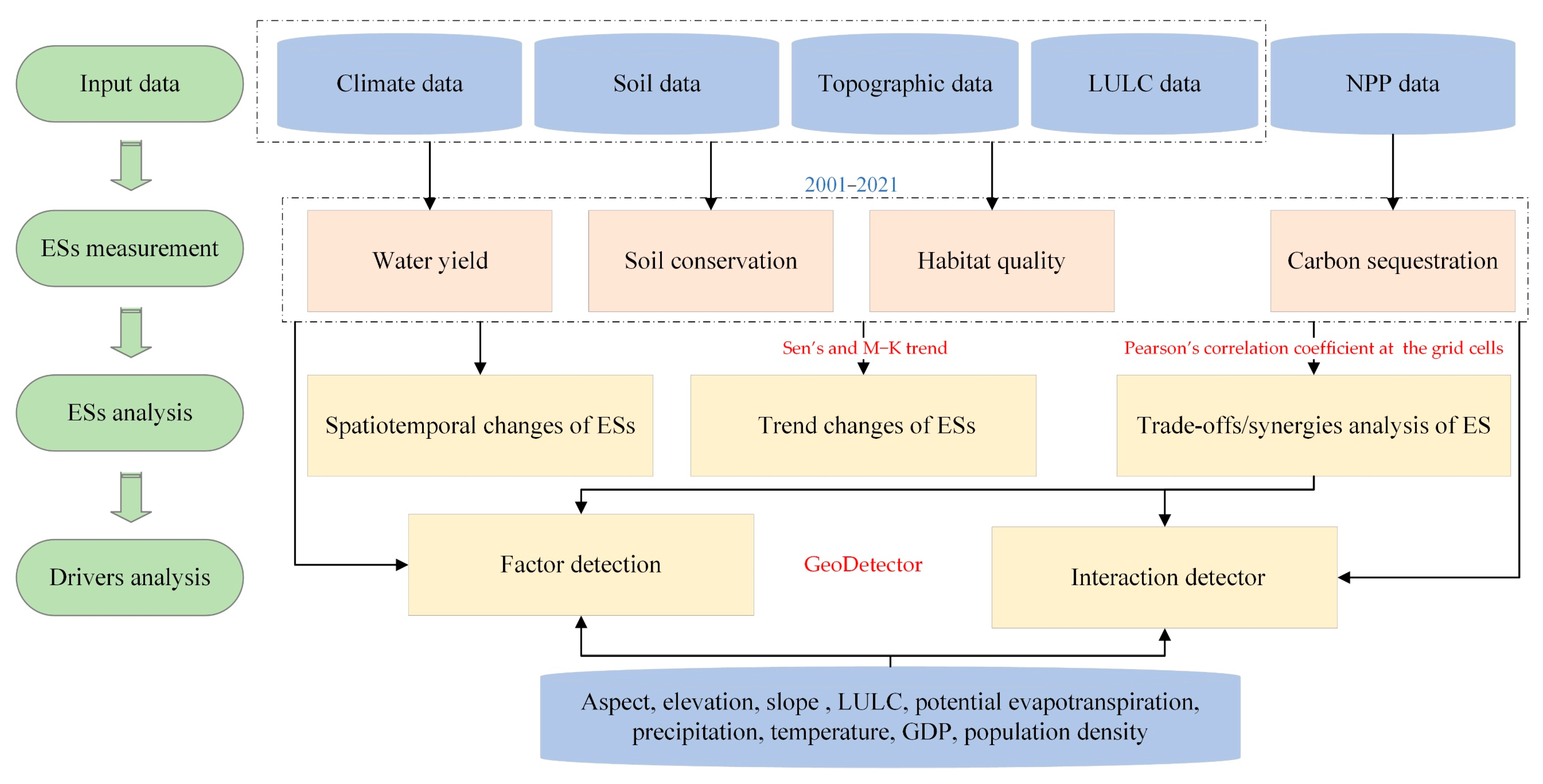
Meteorological, soil, LULC, digital terrain model (DTM), net primary productivity (NPP), and socio-economic datasets were selected in this study and developed using the unified geographic coordinate system with a spatial resolution of 1 km (Table 1). (1) The meteorological measurements were obtained from the CRU TS4.06 datasets after the accuracy test of the measured station data, including monthly precipitation, potential evapotranspiration, and mean temperature. The annual scale meteorological data between 2001 and 2021 were obtained from the monthly data (the correlation coefficients of annual precipitation and temperature data were more than 0.9 (Figure S1)). (2) Soil datasets were obtained from Harmonized World Soil Database (HWSD) version 1.2, including soil depth, soil sand content, silt content, clay content, and organic carbon content. (3) The MCD12Q1 datasets based on the IGBP classification scheme were used as LULC data containing 17 main land cover types. (4) The elevation, slope, and aspect DTM data were acquired from the Shuttle Radar Topography Mission Digital Elevation Model (SRTMDEM). (5) The net primary productivity (NPP) data acquired from MOD17A3HGF version 6.1 were preprocessed by HEG v2.15 (https://wiki.earthdata.nasa.gov/display/DAS/, last accessed 10 August 2023), MATLAB R2020b (https://it.mathworks.com/, last accessed 1 November 2023), and ArcGIS 10.5 (https://www.esri.com/, last accessed 11 January 2024) in terms of splicing, format conversion, re-projection, and resampling. (6) Socio-economic data, including GDP data in 2019 and POD data in 2020, were mainly used to analyze the driving factors of each ES. Figure 2 shows the study flow chart. All data were transformed to a uniform projection coordinate system (WGS_1984_UTM_Zone_48N) and were resampled to a spatial resolution of 1 km.

Table 1.
The essential data for this study.

Figure 2.
Flowchart of this study.
2.3. Methods
2.3.1. ES Assessment Methods
Water yield (WY), carbon sequestration (CS), soil conservation (SC), and habitat quality (HQ) were selected to evaluate ESs in the YZRB and the YRB. All ES models from 2001 to 2021 were output at the YZRB and the YRB grid cells with a spatial resolution of 1km.
(1) The InVEST WY model is a quantitative evaluation method based on the Budyko hydrothermal coupling equilibrium assumption [62], which provides an effective method for WY estimation at high spatial resolution and different scales [63]. The results can be presented as shapefiles, tables, and grid maps. The WY is obtained by subtracting the total actual evapotranspiration from the total precipitation per unit area [64]. The quantitative description is as follows:
where Equations (1)–(6), , , and are the total annual WY (mm), the annual evapotranspiration (mm), and the average annual precipitation (mm) of grid unit , respectively; is the ratio of annual evapotranspiration to average annual precipitation; represents the potential evapotranspiration; and represent the reference crop evapotranspiration and its coefficient, respectively; represents a nonphysical empirical fitting parameter of natural climate-soil properties; is the available water content of plants and is used to determine the amount of water stored and released by the soil for vegetation growth, which is calculated as the difference between the field water holding capacity and the wilting point; is the Zhang parameter that, when set as 7, aligns the average annual WY simulated by InVEST model with the runoff depth results published in the bulletin (http://www.cjw.gov.cn/zwzc/zjgb/cjlyjxnzhszygb/, accessed on 1 July 2022; http://www.yrcc.gov.cn/other/hhgb/, accessed on 1 July 2022; http://www.mwr.gov.cn/sj/tjgb/szygb/, accessed on 1 July 2022); is the plant available water content, which is determined by the mechanical composition of the soil and the root depth of the vegetation [65]; is the maximum soil depth; is the root depth; and , , , and are equal-weight additions of the upper (0–30 cm) and lower layer (30–100 cm) of the contents of sand (%), silt (%), clay (%), and organic matter (%) in the soil, respectively. In addition, the biophysical parameters of the annual WY module used are listed in Table S1, and the raster data input to the InVEST WY module is shown in Figure S2.
(2) NPP is used to evaluate CS services. Since vegetation captures an average of 1.63 units of carbon per unit of NPP, the following relationship exists between NPP and CS [66]:
where CS is the annual carbon sequestration capacity (unit: ) and NPP is the annual NPP data.
(3) SC reflects the different resistance of different land use types to soil erosion and the different soil retention capabilities under different conditions. SC () equals the difference between potential and actual soil erosion, and the study calculates soil conservation based on the InVEST Sediment Delivery Ratio model:
where in Equations from (8) to (10), RKLS and USLE represent potential soil erosion and actual soil erosion, respectively; R is the rainfall erosion factor (), which was calculated by the rainfall erosivity model based on the annual average rainfall estimation in China [67]; is the annual rainfall (mm) (Equation (11)); K is the soil erodibility factor (), which was calculated by erosion-productivity impact calculator proposed by Williams and Arnold [68] (Equation (12)); LS is the slope–slope length factor; C is the vegetation and management factor, which was calculated using the method proposed by Cai et al. [69], in which in Equation (13) is the vegetation cover; and P is the management factor (soil conservation measure factor), which was designed to the YZRB and the YRB concerning relevant studies and combination with the LULC (Table S2). In addition, in Equation (12), sand, , , and represent the content of sand, silt, clay, and organic carbon in the upper layer of soil (0–30 cm), respectively (unit: %).
(4) The InVEST HQ module combines information about land cover types and biodiversity threats to generate an HQ map, which can intuitively evaluate the regional HQ and the level of degradation. It is calculated as follows:
where is the HQ of grid x in land cover type j, with value ranges from 0 to 1, and the closer the value is to 1, the higher the HQ; indicates the habitat fitness of land cover type j. The k is the half-saturation constant, which is generally set to 1/2 of the maximum habitat degradation value. In this study, a consistent k value of 0.13828, representing 1/2 of the maximum degradation value of the habitat in 2001, was configured across all InVEST models for the same landscape. The z was a normalized constant, and the default value was 2.5. represents the habitat degradation degree of grid x in land cover type j. R represents the number of stress factors; indicates the number of grids occupied by stress factor r. represents the weight of the stress factor r, which is between 0 and 1; represents the stress factor value of the grid (0 or 1); represents the threat degree of grid x to stress factor y; represents the accessibility level of the grid; and represents the sensitivity of habitat type to stress factor. The parameters of HQ threat factors and sensitivity in the YZRB and the YRB are shown in Table S3 and Table S4, respectively.
2.3.2. Trend Analysis
The Sen’s Slope and Mann–Kendall (M–K) trend tests were utilized to identify annual trends and significance in the WY, CS, SC, and HQ. Sen’s and M–K trend tests are non-parametric methods that do not require a specific distribution test for sample data; thus, a combination of the two methods will not be affected by missing values and outliers. Moreover, they are flexible in trend analysis and provide significant tests for long-time series data. The Sen’s slope is calculated as follows:
where is the changing trend of each ES, and and are the ES values of time and , respectively; 0 indicates an increasing trend, and indicates a decreasing trend. After identifying the change trends using Sen’s slope method, the significance of the trend results was tested using the M–K method, which is calculated as follows:
where is the length of the time series. The significance tests of change trends were judged based on Z-value, i.e., |Z| ≥ 1.65, |Z| ≥ 1.96, and |Z| ≥ 2.58 indicated statistical significance at (slightly significant), (moderately significant), and (highly significant), respectively.
2.3.3. Trade-Offs/Synergies Analysis
This study used Pearson’s correlation coefficient (R) to measure the trade-offs and synergies relationship between the two ESs from 2001 to 2021:
where and are two different ESs, respectively; and are the mean values of the corresponding ES, respectively; and n represents the number of years (n = 21). R > 0 indicates a synergistic relationship, while R < 0 indicates a trade-off relationship.
2.3.4. GeoDetector Analysis
The GeoDetector [70,71] can detect spatial differences and reveal the driving forces behind statistical methods. It has been widely used in various research fields [72,73,74]. Therefore, the factor detector and interaction detector of GeoDetector were used to explore the degree of explanation of different driving factors to the spatial heterogeneity of ESs and whether the interaction factors increase or weaken the degree of interpretation of spatial heterogeneity of ESs, respectively. The calculation results of the factor detector include q-statistic and p-value, where the former is the influencing coefficient of the driving factor on the ES and the latter is the significance of the q-statistic results. The calculation of the factor detector is as follows:
where the value is strictly within [0,1] and the larger the q-statistic is, the stronger the impact of the driving factor on the ES. is the variance of the ES; (1, …, ) is the stratification of variable Y or factor X, i.e., classification or partition. and are units in layer and the whole area, respectively.
The interaction detector can identify the interpretation degree of ES by the interaction results between different driving factors, which was evaluated by first calculating the q-statistics of factors X1 and X2 on ES, and then calculating the q-statistics on ES during the interaction. The interaction relationships include nonlinear weakening (q(X1∩X) < Min(q(X1),q(X2))), single factor nonlinear weaken (Min(q(X1),q(X2)) < q(X1∩X) < Max(q(X1),q(X2))), bi-factor enhancement (q(X1∩X) > Max(q(X1),q(X2))), independent (q(X1∩X) = q(X1) + q(X2)), and nonlinear enhancement (q(X1∩X) > q(X1) + q(X2)).
In the study, nine driving factors of natural environmental factors and socio-economic factors were selected based on previous studies [12,63], specifically including aspect (ASPECT), elevation (DEM), slope (SLOPE), LULC, potential evapotranspiration (PET), precipitation (PRE), temperature (TEM), GDP, and POD. The GD package in R 4.3.1 (https://CRAN.R-project.org/package=GD, accessed on 26 August 2023) was used optimally to discretize continuous variables (nine driving factors) and to complete the analysis of ESs’ driving mechanisms.
3. Results
3.1. Spatiotemporal and Trend Changes of ESs
3.1.1. Spatiotemporal Changes of ESs
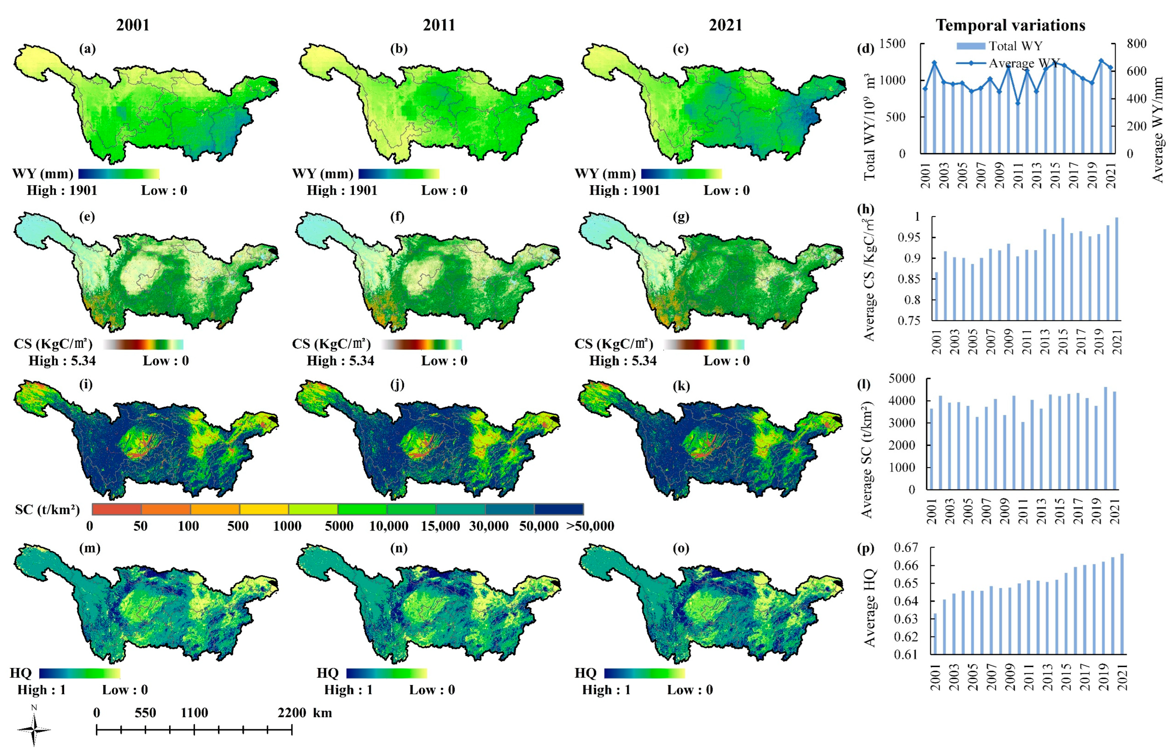
Figure 3 and Figure 4 show the spatial distribution and temporal changes of four ESs (WY, CS, SC, and HQ) in the YZRB and the YRB from 2001 to 2021. In the YZRB (Figure 3), the average annual WY gradually increased from west to east (upstream to downstream), with the eastern part of the basin reaching a high average WY of up to 1678 mm. The CS showed fluctuating increasing changes from 2001 to 2021, with a multi-year average CS of 0.935 KgC/m2 and the lowest and highest values mainly distributed in the northwest and southwest, respectively. High-SC values were predominantly in the central YZRB, with a multi-year average of 3952.38 t/km2. High-HQ areas were primarily located in the western region, with a multi-year average value of 0.652.
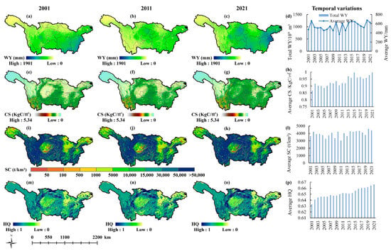
Figure 3.
Spatial distributions and temporal variations of average annual ESs in the YZRB. WY in (a) 2001, (b) 2011, and (c) 2021; CS in (e) 2001, (f) 2011, and (g) 2021; SC in (i) 2001, (j) 2011, and (k) 2021; HQ in (m) 2001, (n) 2011, and (o) 2021; Annual average changes of (d) WY, (h) CS, (l) SC, and (p) HQ from 2001 to 2021.
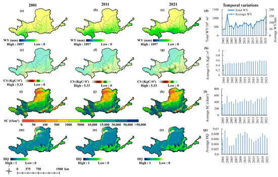
Figure 4.
Spatial distributions and temporal variations of average annual ESs in the YRB. WY in (a) 2001, (b) 2011, and (c) 2021; CS in (e) 2001, (f) 2011, and (g) 2021; SC in (i) 2001, (j) 2011, and (k) 2021; HQ in (m) 2001, (n) 2011, and (o) 2021; Annual average changes of (d) WY, (h) CS, (l) SC, and (p) HQ from 2001 to 2021.
In the YRB (Figure 4), the average WY increased from north to south, but the highest value was only 599 mm, which is much smaller than that in the YZRB. The CS decreased gradually from southeast to northwest, with a multi-year average value of 0.525 KgC/m2. The SC decreased mainly from southwest to northeast, with a multi-year average value of 443.37 t/km2. The average HQ was lowest in the northern regions with barren type, followed by the southern regions with croplands. Conversely, high-HQ areas were mainly located in the central areas where grasslands and some forests were distributed. In summary, the ESs displayed noticeable differences across different basins during the same period or within the same basin at other times.
3.1.2. Trend Changes of ESs
Significant spatial disparities of the four ESs were observed in both basins using the Sen’s slope and the M–K trend test (Figure 5). In the YZRB, the increasing trends of WY exhibited high () and moderate significance (), accounting for 9.24% and 12.74%, respectively, mainly in the central regions (e.g., eastern Sichuan, central Chongqing, and southern Jiangxi). Conversely, highly significant decreases were primarily distributed in the western YZRB (e.g., western Sichuan and northwest Yunnan). The CS increasing trends accounted for approximately 83.44%, with 38.15% exhibiting highly significant increases (e.g., eastern Sichuan and southern Qinghai). Nevertheless, the CS decreased across 14.83% of the YZRB, with highly and moderately significant decreases observed in only 1.40% and 1.52%, primarily in the southern YZRB. The SC increasing trends accounted for 79.12% of the YZRB, including highly (11.40%) and moderately (12.39%) significant increases, mainly in the central and eastern regions. However, 1.83% of the area exhibited a significant SC decrease, mainly in the northern part. The HQ increased in 47.72% of the YZRB, primarily in the central region (24.91% highly significant). However, approximately 33.62% of the YZRB exhibited decreasing HQ trends, with 11.96% experiencing highly significant decreases.
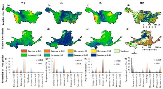
Figure 5.
Spatial trend changes of four ESs from 2001 to 2021. The trend changes of (a) WY, (b) CS, (c) SC, and (d) HQ in the YZRB; The trend changes of (e) WY, (f) CS, (g) SC, and (h) HQ in the YRB; The proportion of area for each trend grade in (i) WY, (j) CS, (k) SC, and (l) HQ.
In the YRB, the WY exhibited highly and moderately significant increases, totaling 10.11% and 22.06%, mainly in the south (e.g., southeastern Qinghai and southern Gansu). The CS of 94.84% area experienced increasing trends, with 62.88% showing highly significant () increases (e.g., Shaanxi, eastern Shanxi, and eastern Gansu). The SC increased across 89.29% of the YRB, with 7.28% displaying highly significant and 18.80% moderately significant increases, primarily in the southern regions. The HQ of 29.82% of the YRB displayed improvements, mainly in the north (18.10% highly significant), while 35.65% exhibited decreases, primarily in the southern urban and agricultural zones (21.86% highly significant). Four ESs of both basins showed an overall improvement trend.
3.2. Trade-Offs/Synergies Analysis of ES
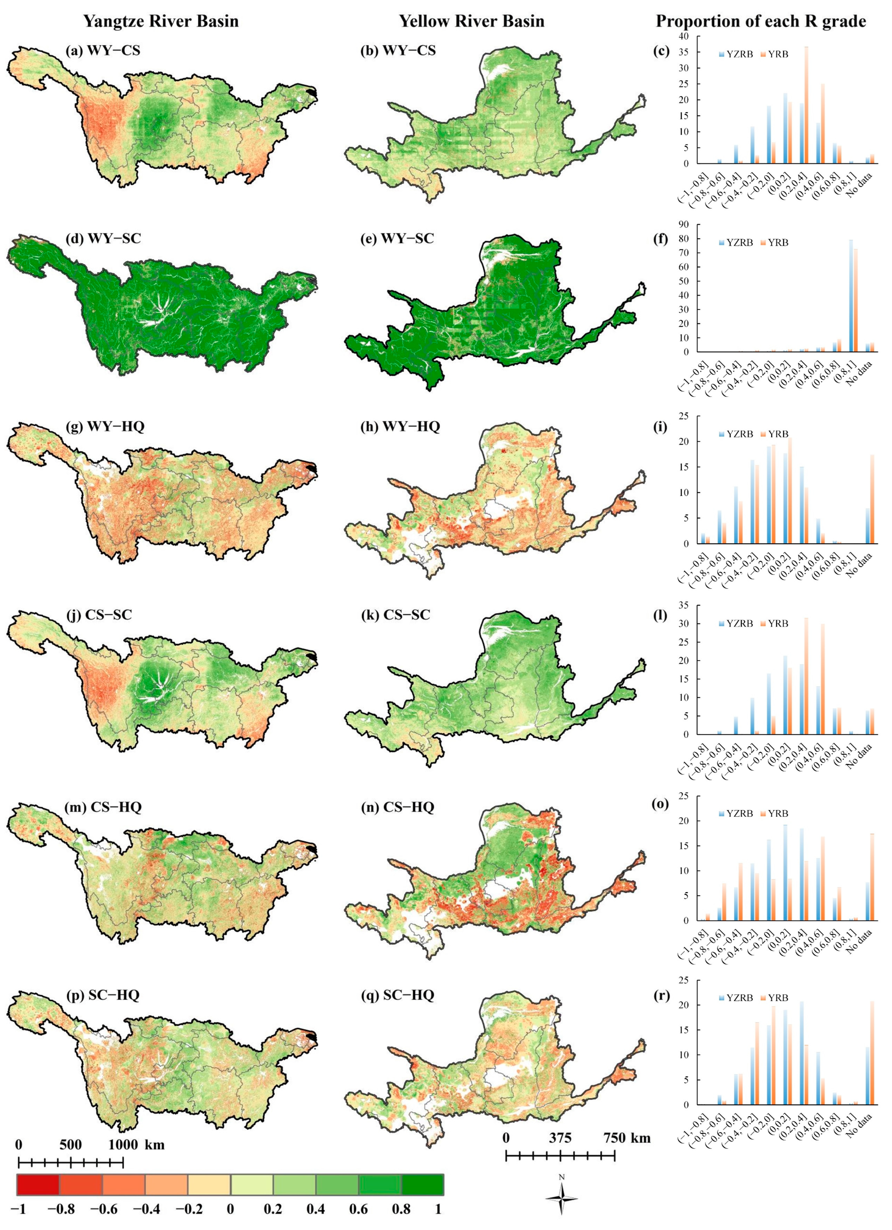
Figure 6 illustrates the trade-off and synergistic relations among ESs in the YZRB and the YRB. The relationship of WY–CS indicated coexistence synergy and trade-off dynamics. In the YZRB, synergies (61.04%) were mainly distributed in the central regions (e.g., eastern Sichuan, Chongqing, Hubei, and Jiangsu), whereas trade-offs (37.02%) were primarily concentrated in western Sichuan and southern Jiangxi. In the YRB, 86.69% of the area exhibited a positive correlation, with significant synergy regions mainly in the north and east. For WY–SC, the positively correlated areas covered 92.28% and 89.36% of the YZRB and the YRB, respectively, with the strongest correlation in the (0.8–1) range, signifying a robust synergy where an increase in one ES promoted the other. For WY–HQ, negatively correlated areas accounted for 55.04% and 48.31% of the YZRB and the YRB, respectively, whereas positively correlated areas constituted 38.11% and 34.29%, indicating a trade-off relationship as the primary interaction. Some regions exhibited an ineffective trade-off/synergy relationship, possibly attributed to stable land cover and unchanging HQ values. For CS–SC, negative correlations covered 32.25% and 6.18% of the YZRB and the YRB, respectively, distributed in the western regions (e.g., western Sichuan) and southeastern areas (e.g., Jiangxi) of YZRB. Positive correlations covered 61.26% and 86.81% of the YZRB and the YRB, respectively, mainly located in the northern and eastern regions of the YRB and eastern Sichuan, Chongqing, and Hubei of the YZRB. For CS–HQ, the YZRB featured an interplay of trade-off (37.19%) and synergy (55.12%) relationships, with a higher synergy in the central YZRB. In the YRB, synergy (44.45%) prevailed in the north, whereas trade-off (38.09%) dominated the south. For SC–HQ, trade-off areas comprised 35.48% (YZRB) and 43.29% (YRB) of their respective basin areas, whereas synergy areas covered 53.03% (YZRB) and 35.96% (YRB). However, these relationships in both basins were primarily characterized by weak trade-offs and synergies scattered across regions.

Figure 6.
The correlation coefficients (R) among multiple ESs from 2001 to 2021 (blank areas in the study area are invalid areas). The R of (a) WY–CS, (d) WY–SC, (g) WY–HQ, (j) CS–SC, (m) CS–HQ, and (p) SC–HQ in the YZRB; The R of (b) WY–CS, (e) WY–SC, (h) WY–HQ, (k) CS–SC, (n) CS–HQ, and (q) SC–HQ in the YRB; The proportion of each R grade (Unit: %) of (c) WY–CS, (f) WY–SC, (i) WY–HQ, (l) CS–SC, (o) CS–HQ, and (r) SC–HQ.
3.3. Driving Factors Analysis in Different ESs
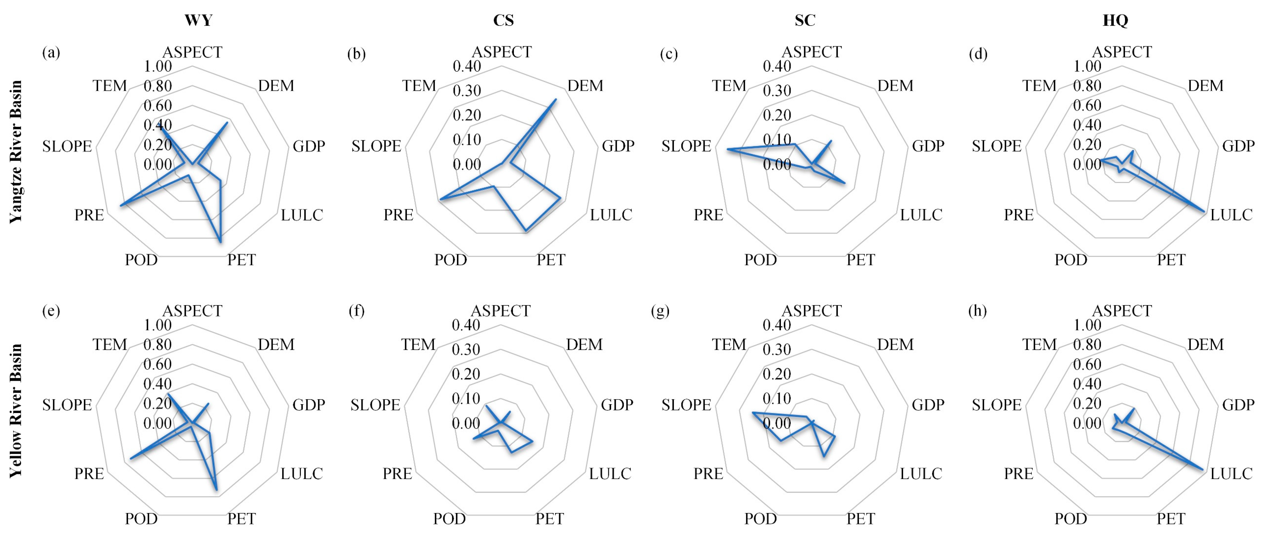
In this study, GeoDetector factor detection was employed to analyze the impact of nine dependent variables on four ESs (taking 2021 as an example), revealing effecting coefficients (q-statistic values) and significance levels (p-value, all < 0.0001) (Figure 7). For WY, PRE and PET remained the most influential driving factors in both basins, playing significant roles in WY services, whereas the contributions of SLOPE, GDP, and ASPECT to the WY in both basins were relatively limited. In addition, the overall influence of each driving factor on WY was more significant in the YZRB than in the YRB. For CS, DEM, PET, PRE, and LULC were the critical factors in the YZRB, with DEM having the most significant influence (q = 0.345), whereas other factors showed a slight impact (q < 0.1). LULC, PET, and PRE were primary factors in the YRB, but their influence was relatively low (q < 0.2), and other factors had small contributions (q < 0.1). For SC, SLOPE was the leading factor in both basins. In the YZRB, LULC, DEM, and TEM were also influenced factors, whereas other factors had a minor impact (q < 0.1). In the YRB, PET, PRE, and LULC played an influential role in SC, but their influence was limited (q < 0.2). For HQ, LULC was the dominant factor in the YZRB and the YRB, with high q-values (0.91 and 0.92, respectively). In summary, the factor detection results highlighted variations in dominant factors across ecosystems.
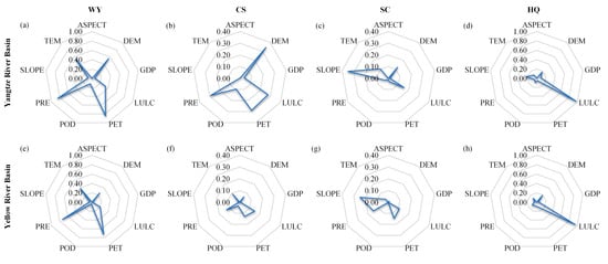
Figure 7.
Factor detection results of four ESs in the YZRB (a–d) and the YRB (e–h) in 2021. The values on the axis of each radar diagram represent the q-statistic values.
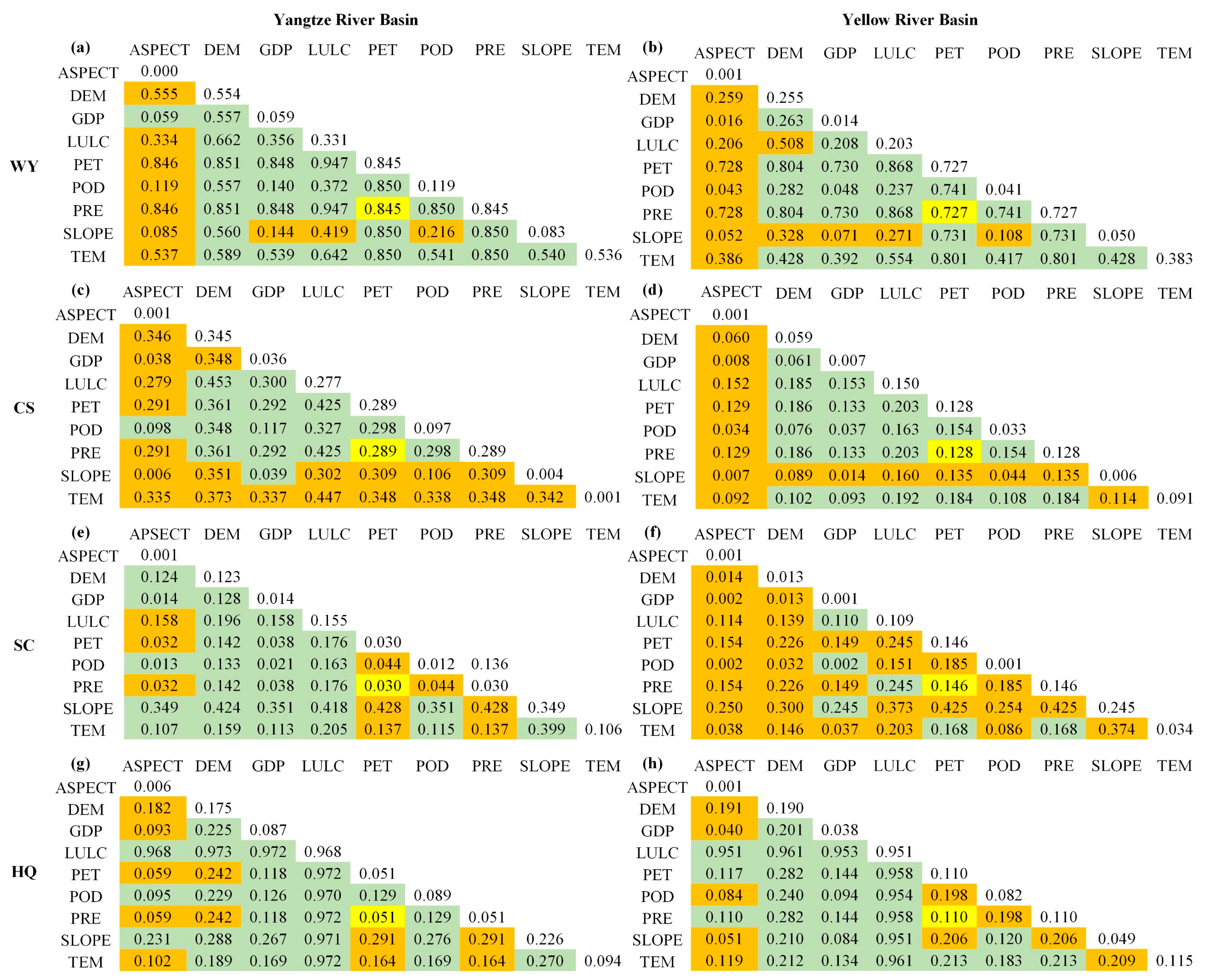
The interaction detection (Figure 8) revealed that pairs of driving factors had a more significant influence on ESs than individual factors. For WY, LULC∩PRE (LULC∩PET) had the most significant influence in the YZRB and the YRB, each with a q-value of 0.947 and 0.868, respectively, closely followed by DEM∩PRE (DEM∩PET). Additionally, 9 (YZRB) and 13 (YRB) pairs of driving factors exhibited nonlinear enhancement, primarily involving the interaction between aspect or slope and other factors. For CS in the YZRB, the most significant interaction was DEM∩LULC (q = 0.453), followed by LULC∩TEM (q = 0.447). Moreover, the interaction between TEM, ASPECT, or SLOPE and most factors significantly boosted CS services in a nonlinear enhancement. For CS in the YRB, LULC∩PRE and LULC∩PET had the most substantial interaction (q = 0.203), while interactions between SLOPE or ASPECT with any factor enhanced the explanatory power through nonlinear enhancement. For SC in the YZRB, interactions demonstrated nonlinear (9 pairs) and bio-factor (25 pairs) enhancements, among which SLOPE∩PRE and SLOPE∩PET had significant impacts with q-values of 0.428. For SC in the YRB, interactions were mainly nonlinear (29 pairs) or bio-factor (6 pairs) enhancements, with SLOPE∩PRE and SLOPE∩PET being the most robust driving factor pairs. For HQ in the YZRB, interactions mainly strengthen HQ by nonlinear (11 pairs) or bio-factor (24 pairs) enhancements, with LULC∩DEM having the most effective influence (q = 0.973), followed by interactions of LULC with PET, PRE, and TEM, each at q = 0.972. For HQ in the YRB (Figure 8h), the most potent interactions were LULC∩DEM and LULC∩TEM, both with q-values of 0.961, followed by LULC∩PET and LULC∩PRE, both at q = 0.958.
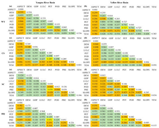
Figure 8.
Interaction detection results of four ESs in the YZRB (a,c,e,g) and the YRB (b,d,f,h) in 2021 using GeoDetector. The values in the table represent the q-statistic values of each ES pair. The orange, green, and yellow fillings represent nonlinear enhancement, bio-factor enhancement, and independence, respectively, and the unfilled numbers represent the single factor detection.
3.4. Driving Factors Analysis of Trade-Offs/Synergies in Different ESs
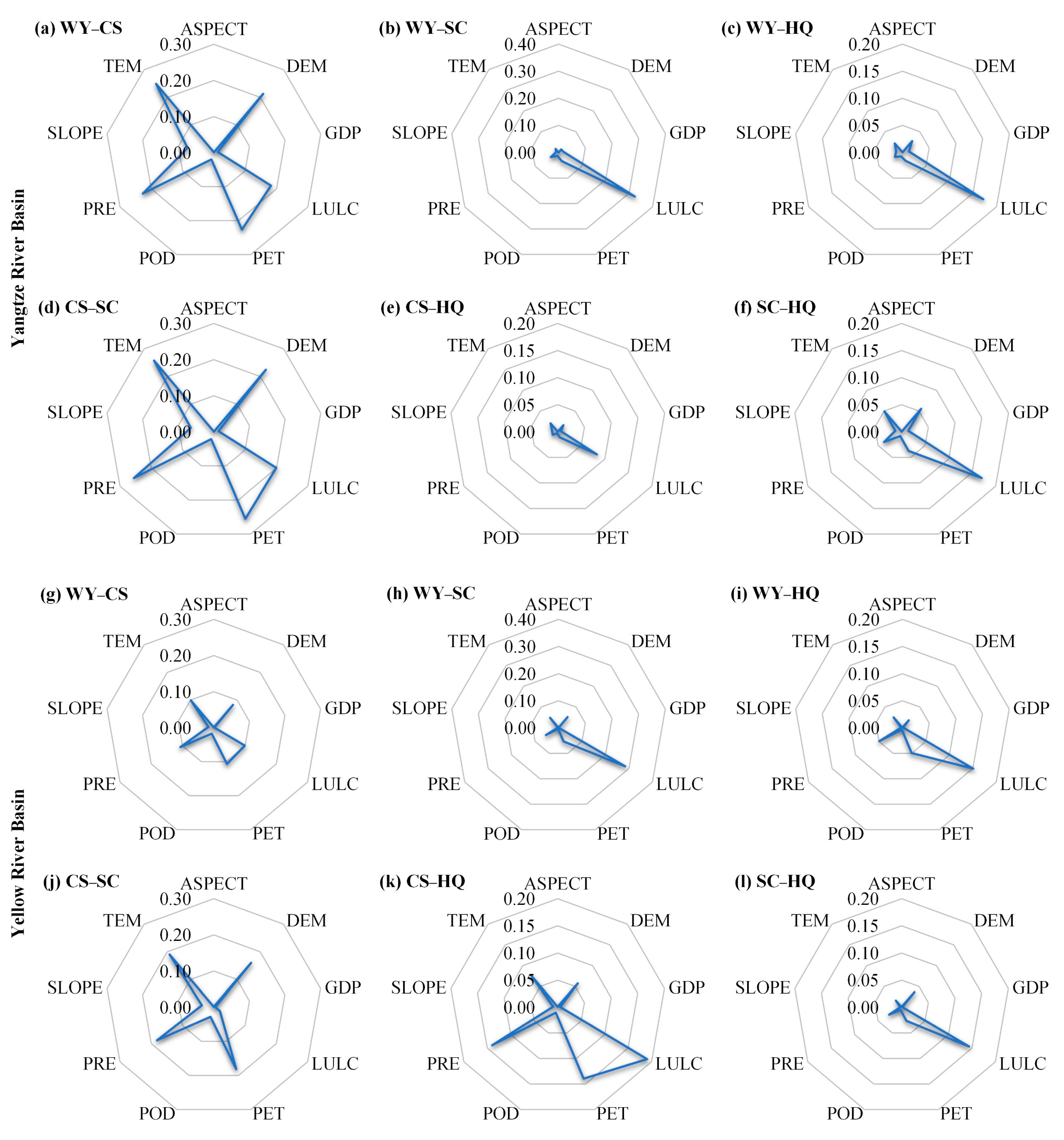
Factor detection results demonstrated that varying driving factors influence trade-off/synergy relationships between ESs in the YZRB and the YRB, with generally more notable impacts in the YZRB (Figure 9). For WY–CS in the YZRB, DEM, LULC, PET, PRE, and TEM played major roles, with respective q-values of 0.212, 0.182, 0.227, 0.227, and 0.249, while in the YRB, only PRE and PET had q-values exceeding 0.1. For WY–SC, WY–HQ, and SC–HQ, LULC had higher q-values than other factors in both basins. Specifically, q-values in the YZRB were 0.324, 0.172, and 0.170 for the three relationships, while in the YRB, they were 0.284, 0.151, and 0.144, respectively. For CS–SC, key factors were LULC, DEM, PET, PRE, and TEM, similar to those influencing the WY–CS relationship. However, for CS–HQ, driving factors had limited impact in the YZRB, with q-values all being below 0.1, whereas LULC, PRE, and PET were the primary drivers in the YRB. Typically, LULC emerged as a dominant factor shaping trade-offs and synergies among ESs in both basins, underscoring its crucial role in ES dynamics.
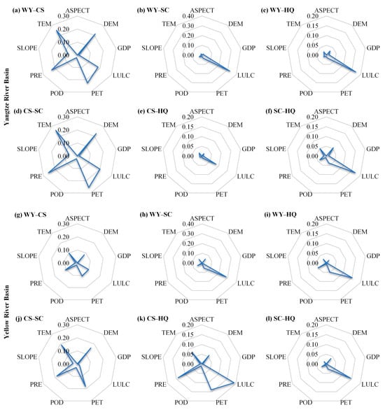
Figure 9.
Factor detection results of the trade-offs/synergies among 4 ESs in the YZRB (a–f) and the YRB (g–l) from 2001 to 2021. The values on the axis of each radar diagram represent the q-statistic values.
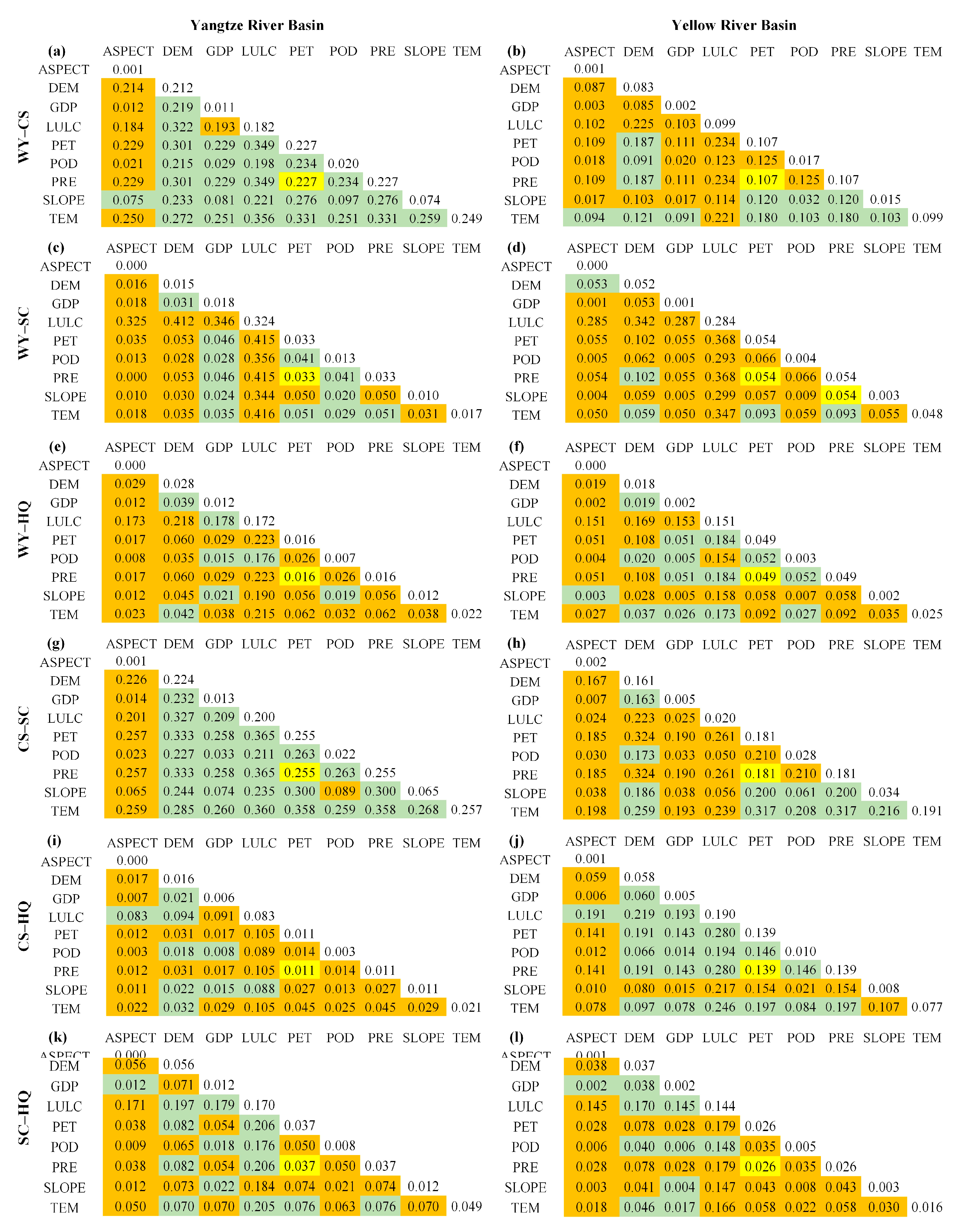
Interaction detection revealed that except for the PRE∩PET, which independently explained trade-offs/synergies in six ES pairs, interactions among other driving factors increased explanatory power for these pairs (Figure 10). For WY–CS, LULC∩TEM had the most significant influence in the YZRB (q = 0.356), while LULC∩PRE and LULC∩PET were dominant in the YRB (q = 0.234). The WY–SC in the YZRB showed 23 pairs of factors with nonlinear enhancements in explanatory power, primarily driven by influential LULC interactions, notably LULC∩TEM (q = 0.416). The WY–SC in the YRB had 30 pairs of factors’ nonlinear enhancements, the most significant being LULC∩PRE and LULC∩PET (q = 0.368). For WY–HQ, LULC∩PRE and LULC∩PET had the most significant explanatory power, with q-values of 0.223 (YZRB) and 0.184 (YRB). For CS–SC in the YZRB, most factor interactions, except for ASPECT and SLOPE∩POD, generally strengthened the explanation nonlinearly, with LULC∩PRE and LULC∩PET having the most significant influence (q = 0.356). For CS–SC in the YRB, DEM∩PET and DEM∩PRE had the most significant impact (q = 0.324). For CS–HQ, YZRB had 26 pairs increasing explanation nonlinearly, but the highest q-value was only 0.105 (LULC∩TEM). YRB had 14 pairs increasing explanation nonlinearly, with LULC∩PRE and LULC∩PET having the most considerable influence on CS–HQ (q = 0.280). For SC–HQ, LULC∩PRE and LULC∩PET were more explanatory, with q-values of 0.206 (YZRB) and 0.179 (YRB).
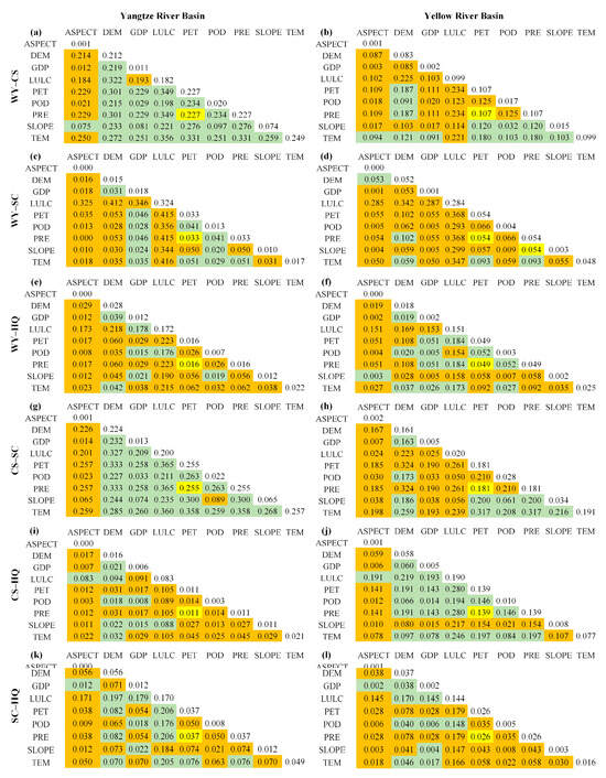
Figure 10.
Interaction detection results of 6 pairs of trade-offs/synergies between ESs in the YZRB (a,c,e,g,i,k) and the YRB (b,d,f,h,j,l) from 2001 to 2021. The values in the table represent the q-statistic values of each ES pair. The orange, green, and yellow fillings represent nonlinear enhancement, bio-factor enhancement, and independence, respectively, and the unfilled numbers represent the single factor detection.
4. Discussion
4.1. Explanation of Influencing Factors on Spatio-Temporal Dynamics of ESs
Factor detectors were used to analyze the driving forces of four ESs, revealing that different dominant factors influence each ES. In this study, the WY was influenced by multiple factors, including precipitation, potential evapotranspiration, elevation, temperature, and LULC (Figure 7), which constituted a complex process driven by the coupling of these various factors [64]. Climate factors had a more significant impact on WY services than anthropogenic factors [12,75], particularly the direct influence of precipitation on WY (Figure 7a,c). The WY from 2001 to 2021 all showed increasing changes with increasing precipitation grades (Figure S3), and both exhibited similar spatial distribution patterns, with regions receiving higher precipitation (e.g., eastern YZRB) generally having higher WY (Figure S2a). Furthermore, existing research has shown a close relationship between potential evapotranspiration and actual evapotranspiration, both of which influence WY services [64], corroborating the findings of our study. The influence of LULC on WY, while individually less significant than climate factors in both basins, was notably strengthened by its interaction with precipitation (Figure 8a), which is consistent with the findings of Yang et al. [76].
Elevation and LULC were the main factors affecting CS in the YZRB and the YRB, respectively. The distribution of CS in the YZRB exhibited an initially increasing trend and then a decreasing trend with rising elevation (Figure S4). Higher elevation in natural forests reduces human disturbance, resulting in longer vegetation growth, greater biomass, and increased CS capacity. However, in unaffected or secondary forests, higher elevations decline above-ground biomass and CS capacity [77]. Hu et al. [78] identified that elevation significantly impacted the CS in the Sichuan Basin. Regarding the YZRB, the interaction between LULC and elevation significantly improved the explanatory power for CS. Sha et al. [79] indicated that LULC significantly impacts CS and emissions. Kafy et al. [80] demonstrated that a decrease in vegetation cover reduces CS capacity, underscoring the importance of effective land use planning and management strategies to minimize the environmental impacts of human activities on CS capacity. In the YRB, increased CS was mainly observed in vegetation regions, with LULC changes from 2001 to 2021 showing growth in grasslands, forests, and croplands, among other vegetation cover types (Figure S5).
Slope emerged as the primary factor explaining SC, and the maximum SC capacity in both basins was observed in areas with slopes exceeding 25° (Figure S6), with SC capacity increasing with slope steepness [12,81]. The interaction between slope and precipitation held substantial explanatory power for SC, aligning with the results of Li et al. [82]. However, some studies suggested that soil erosion could intensify with steeper slopes [56], as high-slope areas were more susceptible to erosional forces, potentially affecting SC. Human activities, like land expansion, could disrupt soil and water conservation environments, altering spatial patterns of SC and impairing its effectiveness [83]. Therefore, ongoing support for ecological engineering initiatives, especially those targeting slope restoration, remained crucial to bolstering SC capabilities in priority conservation areas.
LULC wielded a dominant influence on HQ, with deciduous and broadleaf forests showing the highest quality, followed by water bodies, permanent wetlands, and grasslands, whereas cultivated land demonstrated the lowest quality (Figure S7). Previous research consistently affirmed that forests, shrublands, and grasslands were associated with higher HQ due to their favorable ecological conditions and reduced habitat fragmentation, making them suitable for diverse flora and fauna. Increasing the extent of these land types significantly enhanced HQ services [34]. However, human-induced land cover changes, like urban expansion and cultivation, reduced patch connectivity and landscape fragmentation, resulting in lower HQ in areas with intense human activities, especially in croplands [82]. Changes in LULC from 2001 to 2021 in both basins showed a significant expansion of forests and a slight cropland reduction in the YZRB (Figure S5), aligning with the overall upward trend in HQ.
4.2. Explanation of Trade-Offs/Synergies among ESs
Several ESs exhibited both synergistic and trade-off relationships in both basins. In the YRB, ESs like WY–CS, WY–SC, CS–SC, and CS–HQ exhibited stronger synergistic relationships, whereas trade-offs were dominant in WY–HQ and SC–HQ. Similarly, in the YZRB, most ESs primarily exhibited synergistic relationships, except for the trade-off dominance in WY–HQ. In the YRB, increased multi-year precipitation contributed to greater WY, promoting plant growth, biomass, and, subsequently, CS, indicating a synergistic relationship between WY and CS. In the YZRB, particularly in southern Sichuan, reduced multi-year precipitation decreased WY, leading to an increasing trade-off of WY–CS. Previous research indicated that expanding vegetation cover could enhance CS, but increasing evapotranspiration and decreasing available groundwater could reduce WY [84]. In addition, higher WY, through changes in land use or agricultural practices, may reduce carbon storage and increase carbon emissions. The synergistic relationship between WY and SC stemmed from similar biophysical linkages and soil-hydrological processes [12]. The increased vegetation cover from 2001 to 2021 improved HQ (Figure S7) and raised regional surface evaporation, intensifying the trade-off of HQ–WY [85]. The synergistic relationship of CS–SC corresponded with previous findings [49], as increased vegetation cover enhanced CS capacity and reduced rainfall erosion, improving SC capacity [86]. However, extensive afforestation could introduce a trade-off relationship for CS–SC [87]. Combining the spatial distribution and transition of LULC in the YRB (Figures S2e and S5), conversions of grasslands to croplands in the south reduced HQ and enhanced trade-offs of SC–HQ and WY–HQ. In addition, increasing SC measures often require changes in land use patterns (such as the construction of dams or shelterbelts), which lead to habitat fragmentation and adversely affect the migration and reproduction of wildlife, thereby reducing HQ. Conversely, in the northern YRB, conversions of bare lands into grasslands increased HQ and CS, fostering synergistic interactions. The YZRB transition from grasslands to forests promoted synergy in CS–HQ and SC–HQ.
The YZRB and the YRB displayed differences in trade-offs and synergies among ESs, guiding relevant management and policies. The YZRB, with diverse vegetation, abundant water resources, and a developed economy, fosters mutual ES enhancement. Collaborative efforts optimize resource allocation and ES provision, especially in regions with pronounced synergies. It is imperative to monitor the trade-off relationship between WY and HQ to ensure sustainable water resources and biodiversity conservation. Trade-offs, characterized by uniform land cover, water scarcity, and weaker economic development, especially in WY–HQ and SC–HQ, were more evident in the YRB. Ensuring adequate water resources during dry seasons is vital for maintaining HQ, while effective SC measures can reduce pollutants and improve HQ. Collaboration, especially in the northern and eastern YRB, supports sustainable ES supply and regional economic development.
4.3. Spatiotemporal Scale Effects
The relationships among ESs change over time [50]. However, most studies on ESs and their trade-offs/synergies have been static (single year) or discrete time series, which may lead to misinterpretation of the interrelationships between ESs. The correlation coefficient approach, which considers long-time data, can effectively investigate the dynamic evolution of ESs over time and avoid misjudging the unexpected factors and time lag effects in the long-time evolution of ecosystems [88]. Abundant remote sensing and reanalysis data provide critical data for ES spatial evaluation of continuous time series [89]. Therefore, this study explored the continuous long-time series analysis of ESs and their spatial relationship characteristics by combining multi-source remote sensing data and other fundamental data, which made the results more credible.
The relationships among ESs have been shown to vary at different spatial scales. Xu et al. [90] showed that most of the relationships between ESs were robust at all scales, but there may be a tendency for the correlations of ESs at the pixel scale to be more significant than at the county scale. Wang et al. [91] found that the significance of correlations among ESs varied with spatial scales, e.g., CS and HQ showed trade-offs at the pixel scale but synergies at the county scale. The interaction of LULC with other drivers was a major factor driving the relationship between ESs (Figure 10). In contrast, the change of LULC caused by increasing a specific area (such as forest land) at the pixel scale may lead to an increase in developed land in the same area, thus affecting the supply of ESs at the county scale [47]. The relationships among ESs at large scales could not represent these relationships at the more micro-scale. Therefore, the quantification of trade-offs and synergies of continuous time series at the grid cells was a further supplement to the overall trade-offs and synergies at a large scale, which was not only conducive to grasping the trade-offs and synergies across the entire study object but was also conducive to understanding their spatial relationships, which could provide a reference basis for the implementation of more accurate management measures in the basin areas.
4.4. Limitations and Suggestions
The accuracy of InVEST model outcomes relies highly on the input data’s precision and the module parameters’ configuration. Some parameters, such as the biophysical parameters for the WY and SC modules and the threat and sensitivity parameters for the HQ module, are based on existing research. The inherent uncertainties in these parameters can spread into the simulated ES results [36]. Validating these input parameters through field observations can reduce their potential uncertainties and obtain more reliable results, whereas field observations are expensive and typically cover only relatively small areas. The accuracy of this study’s results may also be affected by the LULC data of the MCD12 product, as previous research has shown that complex mountainous terrain and its associated terrain- and elevation-related pixel mixing challenges can introduce uncertainties in such data sets [92]. Although the changes in ESs and their driving mechanisms are explored based on the pixel scale, the spatial resolution of the output data is 1km × 1 km, and higher spatial resolution data should be collected in the future as the input data to InVEST to simulate ESs more accurately. The YZRB and the YRB span diverse climates, vegetation types, and landscapes, but four typical ESs cannot fully represent the overall ecological conditions. Furthermore, ESs are influenced by natural factors and human activities, and the omission of certain factors in current research may lead to variations in ESs. Finally, this study ignores the contribution of human activities to climate factors in analyzing ES drivers. Frequent human activities (such as fossil fuels, greenhouse gases from agricultural and industrial activities, and aerosol emissions) increase the frequency and severity of extreme precipitation events [93], further affecting ESs [94]. Therefore, in the future, it is essential to explore additional factors to understand the drivers (including anthropogenic climate change) behind the trade-offs and synergies of ESs.
Some suggestions are as follows: (1) Emphasize integrated land use planning to balance ecological, productive, and residential spaces, optimize urban land use efficiency, and consider the ecological impact of urban expansion. (2) Conduct scenario analyses to assess the potential impacts of various land use and management strategies on ESs, facilitating informed decision-making and sustainable land use planning. (3) Understand how urban green networks improve landscape connectivity and can enhance ecosystem functions, biodiversity, and related aspects. (4) Encourage interdisciplinary research involving ecologists, geographers, economists, and policymakers to provide a holistic understanding of the complex relationships within ESs.
5. Conclusions
This study employed the InVEST model to estimate WY, SC, and HQ, as well as NPP to calculate CS. Then, it examined their spatiotemporal changes between 2001 and 2021 in the Yangtze and Yellow River Basins. Using GeoDetector for factor and interaction detection, we identified the influence of natural factors and human activities on the four ESs and their trade-offs/synergies. The main conclusions are as follows:
(1) From 2001 to 2021, except for HQ in the YRB, the ESs in both basins showed an overall increasing trend, and the spatial analysis of the ESs revealed different patterns, with ES values being consistently higher in the YZRB. The highest values of WY, CS, SC, and HQ in the YZRB were concentrated in the eastern, southwestern, central, and western regions, whereas the highest values of WY, CS, SC, and HQ in the YRB were concentrated in the southern, southeastern, southwestern and central grass-covered areas, respectively.
(2) Complex trade-off and synergy relationships were observed among the four ESs, with distinct spatial heterogeneity. WY–HQ and SC–HQ in the YRB and WY–HQ in the YZRB were mainly trade-offs, whereas other ESs exhibited synergistic primary relationships. Notably, the most pronounced synergy was shown between WY and SC, with 90% of the study area exhibiting a positive correlation.
(3) Precipitation and potential evapotranspiration were the dominant factors influencing WY. Elevation and LULC were the primary drivers of CS in the YZRB and the YRB, respectively. Slope and LULC played leading factors in SC and HQ in both basins, respectively. Interactions with slope enhanced the explanatory power for SC. The most crucial aspect is that LULC and its interaction with other factors strengthened the explanatory power for WY, CS, HQ, and six pairs of ES trade-off/synergy relationships.
Supplementary Materials
The following supporting information can be downloaded at https://www.mdpi.com/article/10.3390/rs16020411/s1, Figure S1: Accuracy of CRU precipitation and temperature from 2000 to 2020 (n = 7098); Figure S2: The raster data input to the InVEST water yield module; Figure S3: The annual average changes of WY in the YZRB (a) and the YRB (b) under different precipitation gradient grades (unit: m); Figure S4: The annual average changes of CS in the YZRB (a) and the YRB (b) under different elevation gradient levels (unit: m); Figure S5: The transition of LULC based on MCD12Q1 in the YZRB and the YRB from 2001 to 2021; Figure S6: The annual average changes of SC in the YZRB (a) and the YRB (b) under different slope gradient levels (unit: °); Figure S7: The annual average changes of HQ in the YZRB (a) and the YRB (b) under different LULC types. Table S1: Biophysical parameters used in the InVEST water yield model; Table S2: Biophysical parameters used in the InVEST Sediment Delivery Ratio model; Table S3: The threat factor parameters of habitat quality (HQ); Table S4: The sensitive parameters of habitat quality (HQ).
Author Contributions
Conceptualization, Y.Y.; methodology, Y.Y.; software, Y.Y.; validation, Y.Y.; formal analysis, Y.Y.; investigation, Y.Y.; resources, Y.Y. and L.B.; data curation, Y.Y.; writing—original draft preparation, Y.Y.; writing—review and editing, Z.X., L.B. and H.D.; visualization, Z.X.; supervision, L.B.; project administration, H.D.; funding acquisition, Y.Y. and H.D. All authors have read and agreed to the published version of the manuscript.
Funding
This research was supported by the Scientific Research Foundation Project of Yunnan Provincial Department of Education, grant number 2022J0977, the Nanjing Normal University Doctoral Dissertation Excellent Topic Funding Program, grant number YXXT21-042, and the China Scholarship Council, grant number 202206860014.
Data Availability Statement
The data presented in this study are contained within the article.
Acknowledgments
We are greatly grateful for the support of the funds and projects. We are also very grateful to the anonymous reviewers and editors for their thoughtful review comments and suggestions which have significantly improved this article.
Conflicts of Interest
The authors declare no conflicts of interest.
Abbreviation
| ASPECT | aspect |
| CS | carbon sequestration |
| DEM | elevation |
| ES | ecosystem service |
| GDP | gross domestic product |
| GWR | geographically weighted regression |
| HQ | habitat quality |
| HWSD | Harmonized World Soil Database |
| InVEST | Integrated Valuation of ESs and Tradeoffs |
| LISA | Local Indicators of Spatial Association |
| LULC | land use and land cover |
| M–K | Mann–Kendall |
| NPP | net primary productivity |
| PET | potential evapotranspiration |
| POD | population density |
| PRE | precipitation |
| R | Pearson’s correlation coefficient |
| SC | soil conservation |
| SLOPE | slope |
| SWAT | Soil & Water Assessment Tool |
| TEM | temperature |
| WY | water yield |
| YRB | Yellow River Basin |
| YZRB | Yangtze River Basin |
References
- Scherer-Lorenzen, M.; Gessner, M.O.; Beisner, B.E.; Messier, C.; Paquette, A.; Petermann, J.S.; Soininen, J.; Nock, C.A. Pathways for Cross-Boundary Effects of Biodiversity on Ecosystem Functioning. Trends Ecol. Evol. 2022, 37, 454–467. [Google Scholar] [CrossRef] [PubMed]
- Oteros-Rozas, E.; Martín-López, B.; Fagerholm, N.; Bieling, C.; Plieninger, T. Using Social Media Photos to Explore the Relation between Cultural Ecosystem Services and Landscape Features across Five European Sites. Ecol. Indic. 2018, 94, 74–86. [Google Scholar] [CrossRef]
- Piczak, M.L.; Perry, D.; Cooke, S.J.; Harrison, I.; Benitez, S.; Koning, A.; Peng, L.; Limbu, P.; Smokorowski, K.E.; Salinas-Rodriguez, S.; et al. Protecting and Restoring Habitats to Benefit Freshwater Biodiversity. Environ. Rev. 2023, 00, 1–19. [Google Scholar] [CrossRef]
- Costanza, R. Valuing Natural Capital and Ecosystem Services toward the Goals of Efficiency, Fairness, and Sustainability. Ecosyst. Serv. 2020, 43, 101096. [Google Scholar] [CrossRef]
- De Groot, R.; Brander, L.; van der Ploeg, S.; Costanza, R.; Bernard, F.; Braat, L.; Christie, M.; Crossman, N.; Ghermandi, A.; Hein, L.; et al. Global Estimates of the Value of Ecosystems and Their Services in Monetary Units. Ecosyst. Serv. 2012, 1, 50–61. [Google Scholar] [CrossRef]
- Reid, W.V.; Mooney, H.A.; Cropper, A.; Capistrano, D.; Carpenter, S.R.; Chopra, K.; Dasgupta, P.; Dietz, T.; Duraiappah, A.K.; Hassan, R.; et al. Ecosystems and Human Well-Being: Synthesis; Millennium Ecosystem Assessment (Program), Ed.; Island Press: Washington, DC, USA, 2005; ISBN 978-1-59726-040-4. [Google Scholar]
- Ma, Y.; Jiang, Y. Ecosystem-Based Adaptation to Address Urbanization and Climate Change Challenges: The Case of China’s Sponge City Initiative. Clim. Policy 2023, 23, 268–284. [Google Scholar] [CrossRef]
- Cao, S.; Hu, X.; Wang, Y.; Chen, C.; Xu, D.; Bai, T. Understanding Spatial-Temporal Interactions of Ecosystem Services and Their Drivers in a Multi-Scale Perspective of Miluo Using Multi-Source Remote Sensing Data. Remote Sens. 2023, 15, 3479. [Google Scholar] [CrossRef]
- Hein, L.; White, L.; Miles, A.; Roberts, P. Analysing the Impacts of Air Quality Policies on Ecosystem Services; a Case Study for Telemark, Norway. J. Environ. Manag. 2018, 206, 650–663. [Google Scholar] [CrossRef]
- Rendon, P.; Steinhoff-Knopp, B.; Burkhard, B. Linking Ecosystem Condition and Ecosystem Services: A Methodological Approach Applied to European Agroecosystems. Ecosyst. Serv. 2022, 53, 101387. [Google Scholar] [CrossRef]
- Han, W.; Su, X.; Lu, H.; Li, T.; Jin, T.; Zhang, M.; Liu, G. Impacts of Human Activity Intensity on Ecosystem Services for Conservation in the Lhasa River Basin. Ecosyst. Health Sustain. 2023, 9, 88. [Google Scholar] [CrossRef]
- Fang, L.; Wang, L.; Chen, W.; Sun, J.; Cao, Q.; Wang, S.; Wang, L. Identifying the Impacts of Natural and Human Factors on Ecosystem Service in the Yangtze and Yellow River Basins. J. Clean. Prod. 2021, 314, 127995. [Google Scholar] [CrossRef]
- Zhang, Y.; Lu, X.; Liu, B.; Wu, D.; Fu, G.; Zhao, Y.; Sun, P. Spatial Relationships between Ecosystem Services and Socioecological Drivers across a Large-Scale Region: A Case Study in the Yellow River Basin. Sci. Total Environ. 2021, 766, 142480. [Google Scholar] [CrossRef] [PubMed]
- Dang, A.N.; Jackson, B.M.; Benavidez, R.; Tomscha, S.A. Review of Ecosystem Service Assessments: Pathways for Policy Integration in Southeast Asia. Ecosyst. Serv. 2021, 49, 101266. [Google Scholar] [CrossRef]
- Farley, J. The Role of Prices in Conserving Critical Natural Capital. Conserv. Biol. 2008, 22, 1399–1408. [Google Scholar] [CrossRef] [PubMed]
- Cheng, X.; Van Damme, S.; Uyttenhove, P. A Review of Empirical Studies of Cultural Ecosystem Services in Urban Green Infrastructure. J. Environ. Manag. 2021, 293, 112895. [Google Scholar] [CrossRef] [PubMed]
- Christie, M.; Fazey, I.; Cooper, R.; Hyde, T.; Kenter, J.O. An Evaluation of Monetary and Non-Monetary Techniques for Assessing the Importance of Biodiversity and Ecosystem Services to People in Countries with Developing Economies. Ecol. Econ. 2012, 83, 67–78. [Google Scholar] [CrossRef]
- D’Amato, D.; Rekola, M.; Li, N.; Toppinen, A. Monetary Valuation of Forest Ecosystem Services in China: A Literature Review and Identification of Future Research Needs. Ecol. Econ. 2016, 121, 75–84. [Google Scholar] [CrossRef]
- Campbell, D.E.; Garmestani, A.S. An Energy Systems View of Sustainability: Emergy Evaluation of the San Luis Basin, Colorado. J. Environ. Manag. 2012, 95, 72–97. [Google Scholar] [CrossRef]
- Xu, Z.; Wei, H.; Fan, W.; Wang, X.; Huang, B.; Lu, N.; Ren, J.; Dong, X. Energy Modeling Simulation of Changes in Ecosystem Services before and after the Implementation of a Grain-for-Green Program on the Loess Plateau—A Case Study of the Zhifanggou Valley in Ansai County, Shaanxi Province, China. Ecosyst. Serv. 2018, 31, 32–43. [Google Scholar] [CrossRef]
- Villa, F.; Bagstad, K.; Johnson, G.; Voigt, B. Scientific Instruments for Climate Change Adaptation: Estimating and Optimizing the Efficiency of Ecosystem Service Provision. Econ. Agrar. Recur. Nat. 2011, 11, 83–98. [Google Scholar] [CrossRef]
- Jackson, B.; Pagella, T.; Sinclair, F.; Orellana, B.; Henshaw, A.; Reynolds, B.; Mcintyre, N.; Wheater, H.; Eycott, A. Polyscape: A GIS Mapping Framework Providing Efficient and Spatially Explicit Landscape-Scale Valuation of Multiple Ecosystem Services. Landsc. Urban Plan. 2013, 112, 74–88. [Google Scholar] [CrossRef]
- Vorstius, A.C.; Spray, C.J. A Comparison of Ecosystem Services Mapping Tools for Their Potential to Support Planning and Decision-Making on a Local Scale. Ecosyst. Serv. 2015, 15, 75–83. [Google Scholar] [CrossRef]
- Sherrouse, B.C.; Clement, J.M.; Semmens, D.J. A GIS Application for Assessing, Mapping, and Quantifying the Social Values of Ecosystem Services. Appl. Geogr. 2011, 31, 748–760. [Google Scholar] [CrossRef]
- Peh, K.S.-H.; Balmford, A.; Bradbury, R.B.; Brown, C.; Butchart, S.H.M.; Hughes, F.M.R.; Stattersfield, A.; Thomas, D.H.L.; Walpole, M.; Bayliss, J.; et al. TESSA: A Toolkit for Rapid Assessment of Ecosystem Services at Sites of Biodiversity Conservation Importance. Ecosyst. Serv. 2013, 5, 51–57. [Google Scholar] [CrossRef]
- Zaks, I. InVEST. Available online: https://naturalcapitalproject.stanford.edu/software/invest (accessed on 14 September 2023).
- Sharps, K.; Masante, D.; Thomas, A.; Jackson, B.; Redhead, J.; May, L.; Prosser, H.; Cosby, B.; Emmett, B.; Jones, L. Comparing Strengths and Weaknesses of Three Ecosystem Services Modelling Tools in a Diverse UK River Catchment. Sci. Total Environ. 2017, 584–585, 118–130. [Google Scholar] [CrossRef] [PubMed]
- Hamel, P.; Chaplin-Kramer, R.; Sim, S.; Mueller, C. A New Approach to Modeling the Sediment Retention Service (InVEST 3.0): Case Study of the Cape Fear Catchment, North Carolina, USA. Sci. Total Environ. 2015, 524–525, 166–177. [Google Scholar] [CrossRef]
- McMahon, J.M.; Hasan, S.; Brooks, A.; Curwen, G.; Dyke, J.; Ange, C.S.; Smart, J.C.R. Challenges in Modelling the Sediment Retention Ecosystem Service to Inform an Ecosystem Account—Examples from the Mitchell Catchment in Northern Australia. J. Environ. Manag. 2022, 314, 115102. [Google Scholar] [CrossRef]
- Cong, W.; Sun, X.; Guo, H.; Shan, R. Comparison of the SWAT and InVEST Models to Determine Hydrological Ecosystem Service Spatial Patterns, Priorities and Trade-Offs in a Complex Basin. Ecol. Indic. 2020, 112, 106089. [Google Scholar] [CrossRef]
- Dennedy-Frank, P.J.; Muenich, R.L.; Chaubey, I.; Ziv, G. Comparing Two Tools for Ecosystem Service Assessments Regarding Water Resources Decisions. J. Environ. Manag. 2016, 177, 331–340. [Google Scholar] [CrossRef]
- Decsi, B.; Ács, T.; Jolánkai, Z.; Kardos, M.K.; Koncsos, L.; Vári, Á.; Kozma, Z. From Simple to Complex—Comparing Four Modelling Tools for Quantifying Hydrologic Ecosystem Services. Ecol. Indic. 2022, 141, 109143. [Google Scholar] [CrossRef]
- Zeng, J.; Xu, J.; Li, W.; Dai, X.; Zhou, J.; Shan, Y.; Zhang, J.; Li, W.; Lu, H.; Ye, Y.; et al. Evaluating Trade-Off and Synergies of Ecosystem Services Values of a Representative Resources-Based Urban Ecosystem: A Coupled Modeling Framework Applied to Panzhihua City, China. Remote Sens. 2022, 14, 5282. [Google Scholar] [CrossRef]
- Yan, K.; Wang, W.; Li, Y.; Wang, X.; Jin, J.; Jiang, J.; Yang, H.; Wang, L. Identifying Priority Conservation Areas Based on Ecosystem Services Change Driven by Natural Forest Protection Project in Qinghai Province, China. J. Clean. Prod. 2022, 362, 132453. [Google Scholar] [CrossRef]
- Yu, Y.; Sun, X.; Wang, J.; Zhang, J. Using InVEST to Evaluate Water Yield Services in Shangri-La, Northwestern Yunnan, China. PeerJ 2022, 10, e12804. [Google Scholar] [CrossRef] [PubMed]
- Hu, X.; Hou, Y.; Li, D.; Hua, T.; Marchi, M.; Paola Forero Urrego, J.; Huang, B.; Zhao, W.; Cherubini, F. Changes in Multiple Ecosystem Services and Their Influencing Factors in Nordic Countries. Ecol. Indic. 2023, 146, 109847. [Google Scholar] [CrossRef]
- Huang, F.; Zuo, L.; Gao, J.; Jiang, Y.; Du, F.; Zhang, Y. Exploring the Driving Factors of Trade-Offs and Synergies among Ecological Functional Zones Based on Ecosystem Service Bundles. Ecol. Indic. 2023, 146, 109827. [Google Scholar] [CrossRef]
- Zhou, Z.; Robinson, G.M.; Song, B. Experimental Research on Trade-Offs in Ecosystem Services: The Agro-Ecosystem Functional Spectrum. Ecol. Indic. 2019, 106, 105536. [Google Scholar] [CrossRef]
- Wu, F.; Liang, Y.; Peng, S.; Huang, J.; Liu, L. Challenges in Trade-off Governance of Ecosystem Services: Evidence from the Loess Plateau in China. Ecol. Indic. 2022, 145, 109686. [Google Scholar] [CrossRef]
- Li, B.; Chen, N.; Wang, Y.; Wang, W. Spatio-Temporal Quantification of the Trade-Offs and Synergies among Ecosystem Services Based on Grid-Cells: A Case Study of Guanzhong Basin, NW China. Ecol. Indic. 2018, 94, 246–253. [Google Scholar] [CrossRef]
- Yuan, J.; Li, R.; Huang, K. Driving Factors of the Variation of Ecosystem Service and the Trade-off and Synergistic Relationships in Typical Karst Basin. Ecol. Indic. 2022, 142, 109253. [Google Scholar] [CrossRef]
- Yang, J.; Li, J.; Fu, G.; Liu, B.; Pan, L.; Hao, H.; Guan, X. Spatial and Temporal Patterns of Ecosystem Services and Trade-Offs/Synergies in Wujiang River Basin, China. Remote Sens. 2023, 15, 4099. [Google Scholar] [CrossRef]
- Jia, Z.; Wang, X.; Feng, X.; Ma, J.; Wang, X.; Zhang, X.; Zhou, J.; Sun, Z.; Yao, W.; Tu, Y. Exploring the Spatial Heterogeneity of Ecosystem Services and Influencing Factors on the Qinghai Tibet Plateau. Ecol. Indic. 2023, 154, 110521. [Google Scholar] [CrossRef]
- Wang, Y.; Dai, E.; Ge, Q.; Zhang, X.; Yu, C. Spatial Heterogeneity of Ecosystem Services and Their Trade-Offs in the Hengduan Mountain Region, Southwest China. Catena 2021, 207, 105632. [Google Scholar] [CrossRef]
- Li, Y.; Luo, H. Trade-off/Synergistic Changes in Ecosystem Services and Geographical Detection of Its Driving Factors in Typical Karst Areas in Southern China. Ecol. Indic. 2023, 154, 110811. [Google Scholar] [CrossRef]
- Qiao, X.; Gu, Y.; Zou, C.; Xu, D.; Wang, L.; Ye, X.; Yang, Y.; Huang, X. Temporal Variation and Spatial Scale Dependency of the Trade-Offs and Synergies among Multiple Ecosystem Services in the Taihu Lake Basin of China. Sci. Total Environ. 2019, 651, 218–229. [Google Scholar] [CrossRef] [PubMed]
- Bai, Y.; Chen, Y.; Alatalo, J.M.; Yang, Z.; Jiang, B. Scale Effects on the Relationships between Land Characteristics and Ecosystem Services- a Case Study in Taihu Lake Basin, China. Sci. Total Environ. 2020, 716, 137083. [Google Scholar] [CrossRef] [PubMed]
- Wu, X.; Zhang, L.; Gao, L.; Li, Y.; Liu, X. Change and Tradeoff/Synergy Analysis of Watershed Ecosystem Services: A Case Study of Qinghai Lake Basin. Sustainability 2023, 15, 11711. [Google Scholar] [CrossRef]
- Li, G.; Jiang, C.; Gao, Y.; Du, J. Natural Driving Mechanism and Trade-off and Synergy Analysis of the Spatiotemporal Dynamics of Multiple Typical Ecosystem Services in Northeast Qinghai-Tibet Plateau. J. Clean. Prod. 2022, 374, 134075. [Google Scholar] [CrossRef]
- Wang, Z.; Yang, H.; Hu, Y.; Peng, Y.; Liu, L.; Su, S.; Wang, W.; Wu, J. Multifunctional Trade-off/Synergy Relationship of Cultivated Land in Guangdong: A Long Time Series Analysis from 2010 to 2030. Ecol. Indic. 2023, 154, 110700. [Google Scholar] [CrossRef]
- IPBES 2019 Global Assessment on Biodiversity and Ecosystem Services. Available online: https://earthlobbyist.com/ipbes-2019-global-assessment-on-biodiversity-and-ecosystems/ (accessed on 14 September 2023).
- Yu, Y.; Shen, Y.; Wang, J.; Wei, Y.; Nong, L.; Deng, H. Assessing the Response of Vegetation Change to Drought during 2009–2018 in Yunnan Province, China. Environ. Sci. Pollut. Res. 2021, 28, 47066–47082. [Google Scholar] [CrossRef]
- Hasan, S.S.; Zhen, L.; Miah, M.G.; Ahamed, T.; Samie, A. Impact of Land Use Change on Ecosystem Services: A Review. Environ. Dev. 2020, 34, 100527. [Google Scholar] [CrossRef]
- Yu, Y.; Fang, S.; Zhuo, W. Revealing the Driving Mechanisms of Land Surface Temperature Spatial Heterogeneity and Its Sensitive Regions in China Based on GeoDetector. Remote Sens. 2023, 15, 2814. [Google Scholar] [CrossRef]
- Pan, H.; Wang, J.; Du, Z.; Wu, Z.; Zhang, H.; Ma, K. Spatiotemporal Evolution of Ecosystem Services and Its Potential Drivers in Coalfields of Shanxi Province, China. Ecol. Indic. 2023, 148, 110109. [Google Scholar] [CrossRef]
- Wang, H.; Gao, J.; Hou, W. Quantitative Attribution Analysis of Soil Erosion in Different Geomorphological Types in Karst Areas: Based on the Geodetector Method. J. Geogr. Sci. 2019, 29, 271–286. [Google Scholar] [CrossRef]
- Liang, Y.; Xu, C. Knowledge Diffusion of Geodetector: A Perspective of the Literature Review and Geotree. Heliyon 2023, 9, e19651. [Google Scholar] [CrossRef] [PubMed]
- Yang, H.; Zhong, X.; Deng, S.; Xu, H. Assessment of the Impact of LUCC on NPP and Its Influencing Factors in the Yangtze River Basin, China. Catena 2021, 206, 105542. [Google Scholar] [CrossRef]
- Zhang, Y.; Zhao, Z.; Fu, B.; Ma, R.; Yang, Y.; Lü, Y.; Wu, X. Identifying Ecological Security Patterns Based on the Supply, Demand and Sensitivity of Ecosystem Service: A Case Study in the Yellow River Basin, China. J. Environ. Manag. 2022, 315, 115158. [Google Scholar] [CrossRef] [PubMed]
- Kong, L.; Zheng, H.; Rao, E.; Xiao, Y.; Ouyang, Z.; Li, C. Evaluating Indirect and Direct Effects of Eco-Restoration Policy on Soil Conservation Service in Yangtze River Basin. Sci. Total Environ. 2018, 631–632, 887–894. [Google Scholar] [CrossRef]
- Wu, C.; Ma, G.; Yang, W.; Zhou, Y.; Peng, F.; Wang, J.; Yu, F. Assessment of Ecosystem Service Value and Its Differences in the Yellow River Basin and Yangtze River Basin. Sustainability 2021, 13, 3822. [Google Scholar] [CrossRef]
- Budyko, M.I. Climate and Life; International Geophysics Series; Academic Press: New York, NY, USA, 1974; ISBN 978-0-12-139450-9. [Google Scholar]
- Zhang, X.; Zhang, G.; Long, X.; Zhang, Q.; Liu, D.; Wu, H.; Li, S. Identifying the Drivers of Water Yield Ecosystem Service: A Case Study in the Yangtze River Basin, China. Ecol. Indic. 2021, 132, 108304. [Google Scholar] [CrossRef]
- Li, M.; Liang, D.; Xia, J.; Song, J.; Cheng, D.; Wu, J.; Cao, Y.; Sun, H.; Li, Q. Evaluation of Water Conservation Function of Danjiang River Basin in Qinling Mountains, China Based on InVEST Model. J. Environ. Manag. 2021, 286, 112212. [Google Scholar] [CrossRef]
- Zhou, W.; Liu, G.; Pan, J.; Feng, X. Distribution of Available Soil Water Capacity in China. J. Geogr. Sci. 2005, 15, 3–12. [Google Scholar] [CrossRef]
- Hua, T.; Zhao, W.; Cherubini, F.; Hu, X.; Pereira, P. Sensitivity and Future Exposure of Ecosystem Services to Climate Change on the Tibetan Plateau of China. Landsc. Ecol. 2021, 36, 3451–3471. [Google Scholar] [CrossRef]
- Zhang, W.; Fu, J. Rainfall Erosivity Estimation under Different Rainfall Amount. Resour. Sci. 2003, 1, 35–41. [Google Scholar]
- Williams, J.R.; Arnold, J.G. A System of Erosion—Sediment Yield Models. Soil Technol. 1997, 11, 43–55. [Google Scholar] [CrossRef]
- Cai, C.; Ding, S.; Shi, Z.; Huang, L.; Zhang, G. Study of Applying USLE and Geographical Information System IDRISI to Predict Soil Erosion in Small Watershed. J. Soil Water Conserv. 2000, 2, 19–24. [Google Scholar]
- Wang, J.; Li, X.; Christakos, G.; Liao, Y.; Zhang, T.; Gu, X.; Zheng, X. Geographical Detectors-Based Health Risk Assessment and Its Application in the Neural Tube Defects Study of the Heshun Region, China. Int. J. Geogr. Inf. Sci. 2010, 24, 107–127. [Google Scholar] [CrossRef]
- Wang, J.-F.; Zhang, T.-L.; Fu, B.-J. A Measure of Spatial Stratified Heterogeneity. Ecol. Indic. 2016, 67, 250–256. [Google Scholar] [CrossRef]
- Aizizi, Y.; Kasimu, A.; Liang, H.; Zhang, X.; Zhao, Y.; Wei, B. Evaluation of Ecological Space and Ecological Quality Changes in Urban Agglomeration on the Northern Slope of the Tianshan Mountains. Ecol. Indic. 2023, 146, 109896. [Google Scholar] [CrossRef]
- Du, L.; Dong, C.; Kang, X.; Qian, X.; Gu, L. Spatiotemporal Evolution of Land Cover Changes and Landscape Ecological Risk Assessment in the Yellow River Basin, 2015–2020. J. Environ. Manag. 2023, 332, 117149. [Google Scholar] [CrossRef]
- Han, H.; Jian, H.; Liu, M.; Lei, S.; Yao, S.; Yan, F. Impacts of Drought and Heat Events on Vegetative Growth in a Typical Humid Zone of the Middle and Lower Reaches of the Yangtze River, China. J. Hydrol. 2023, 620, 129452. [Google Scholar] [CrossRef]
- Bai, Y.; Ochuodho, T.O.; Yang, J. Impact of Land Use and Climate Change on Water-Related Ecosystem Services in Kentucky, USA. Ecol. Indic. 2019, 102, 51–64. [Google Scholar] [CrossRef]
- Yang, H.; Nie, S.; Deng, S.; Zhou, H.; Zhou, X. Evaluation of Water Yield and Its Driving Factors in the Yangtze River Basin, China. Environ. Earth Sci. 2023, 82, 429. [Google Scholar] [CrossRef]
- Wang, X.; Liu, W. Factors affecting carbon sequestration in forests. For. Ecol. 2021, 40–41. [Google Scholar] [CrossRef]
- Hu, C.; Wang, Z.; Li, J.; Liu, H.; Sun, D. Quantifying the Temporal and Spatial Patterns of Ecosystem Services and Exploring the Spatial Differentiation of Driving Factors: A Case Study of Sichuan Basin, China. Front. Environ. Sci. 2022, 10, 927818. [Google Scholar] [CrossRef]
- Sha, Z.; Bai, Y.; Li, R.; Lan, H.; Zhang, X.; Li, J.; Liu, X.; Chang, S.; Xie, Y. The Global Carbon Sink Potential of Terrestrial Vegetation Can Be Increased Substantially by Optimal Land Management. Commun Earth Environ. 2022, 3, 8. [Google Scholar] [CrossRef]
- Kafy, A.-A.; Saha, M.; Fattah, M.A.; Rahman, M.T.; Duti, B.M.; Rahaman, Z.A.; Bakshi, A.; Kalaivani, S.; Nafiz Rahaman, S.; Sattar, G.S. Integrating Forest Cover Change and Carbon Storage Dynamics: Leveraging Google Earth Engine and InVEST Model to Inform Conservation in Hilly Regions. Ecol. Indic. 2023, 152, 110374. [Google Scholar] [CrossRef]
- Lu, R.; Dai, E.; Wu, C. Spatial and Temporal Evolution Characteristics and Driving Factors of Soil Conservation Services on the Qinghai-Tibet Plateau. Catena 2023, 221, 106766. [Google Scholar] [CrossRef]
- Li, H.; He, R.; Hu, J.; Zhou, Y.; Xie, M.; Deng, W.; Wang, J.; Zhao, W.; Zhang, S.; Jiang, Y.; et al. Identifying Conservation Priority Zones and Their Driving Factors Regarding Regional Ecosystem Services. Environ. Dev. Sustain. 2023, 1–23. [Google Scholar] [CrossRef]
- Xiao, Q.; Hu, D.; Xiao, Y. Assessing Changes in Soil Conservation Ecosystem Services and Causal Factors in the Three Gorges Reservoir Region of China. J. Clean. Prod. 2017, 163, S172–S180. [Google Scholar] [CrossRef]
- Filoso, S.; Bezerra, M.O.; Weiss, K.C.B.; Palmer, M.A. Impacts of Forest Restoration on Water Yield: A Systematic Review. PLoS ONE 2017, 12, e0183210. [Google Scholar] [CrossRef]
- Shao, Y.; Liu, Y.; Li, Y.; Yuan, X. Regional Ecosystem Services Relationships and Their Potential Driving Factors in the Yellow River Basin, China. J. Geogr. Sci. 2023, 33, 863–884. [Google Scholar] [CrossRef]
- Feng, X.; Zhang, T.; Feng, P.; Li, J. Evaluation and Tradeoff-Synergy Analysis of Ecosystem Services in Luanhe River Basin. Ecohydrology 2022, 15, e2473. [Google Scholar] [CrossRef]
- Wang, C.; Wang, S.; Fu, B.; Li, Z.; Wu, X.; Tang, Q. Precipitation Gradient Determines the Tradeoff between Soil Moisture and Soil Organic Carbon, Total Nitrogen, and Species Richness in the Loess Plateau, China. Sci. Total Environ. 2017, 575, 1538–1545. [Google Scholar] [CrossRef] [PubMed]
- Dallimer, M.; Davies, Z.G.; Diaz-Porras, D.F.; Irvine, K.N.; Maltby, L.; Warren, P.H.; Armsworth, P.R.; Gaston, K.J. Historical Influences on the Current Provision of Multiple Ecosystem Services. Glob. Environ. Change 2015, 31, 307–317. [Google Scholar] [CrossRef]
- Braun, D.; Damm, A.; Hein, L.; Petchey, O.L.; Schaepman, M.E. Spatio-Temporal Trends and Trade-Offs in Ecosystem Services: An Earth Observation Based Assessment for Switzerland between 2004 and 2014. Ecol. Indic. 2018, 89, 828–839. [Google Scholar] [CrossRef]
- Xu, S.; Liu, Y.; Wang, X.; Zhang, G. Scale Effect on Spatial Patterns of Ecosystem Services and Associations among Them in Semi-Arid Area: A Case Study in Ningxia Hui Autonomous Region, China. Sci. Total Environ. 2017, 598, 297–306. [Google Scholar] [CrossRef] [PubMed]
- Wang, L.-J.; Gong, J.-W.; Ma, S.; Wu, S.; Zhang, X.; Jiang, J. Ecosystem Service Supply–Demand and Socioecological Drivers at Different Spatial Scales in Zhejiang Province, China. Ecol. Indic. 2022, 140, 109058. [Google Scholar] [CrossRef]
- Shao, Q.; Han, L.; Lv, L.; Shao, H.; Qi, J. Spatiotemporal Variation and Factors Influencing Water Yield Services in the Hengduan Mountains, China. Remote Sens. 2023, 15, 4087. [Google Scholar] [CrossRef]
- Gao, L.; Huang, J.; Chen, X.; Chen, Y.; Liu, M. Contributions of Natural Climate Changes and Human Activities to the Trend of Extreme Precipitation. Atmos. Res. 2018, 205, 60–69. [Google Scholar] [CrossRef]
- Liu, L.; Jiang, Y.; Gao, J.; Feng, A.; Jiao, K.; Wu, S.; Zuo, L.; Li, Y.; Yan, R. Concurrent Climate Extremes and Impacts on Ecosystems in Southwest China. Remote Sens. 2022, 14, 1678. [Google Scholar] [CrossRef]
Disclaimer/Publisher’s Note: The statements, opinions and data contained in all publications are solely those of the individual author(s) and contributor(s) and not of MDPI and/or the editor(s). MDPI and/or the editor(s) disclaim responsibility for any injury to people or property resulting from any ideas, methods, instructions or products referred to in the content. |
© 2024 by the authors. Licensee MDPI, Basel, Switzerland. This article is an open access article distributed under the terms and conditions of the Creative Commons Attribution (CC BY) license (https://creativecommons.org/licenses/by/4.0/).

