Convolutional Neural Network-Based Method for Agriculture Plot Segmentation in Remote Sensing Images

Abstract

Accurate delineation of individual agricultural plots, the foundational units for agriculture-based activities, is crucial for effective government oversight of agricultural productivity and land utilization. To improve the accuracy of plot segmentation in high-resolution remote sensing images, the paper collects GF-2 satellite remote sensing images, uses ArcGIS10.3.1 software to establish datasets, and builds UNet, SegNet, DeeplabV3+, and TransUNet neural network frameworks, respectively, for experimental analysis. Then, the TransUNet network with the best segmentation effects is optimized in both the residual module and the skip connection to further improve its performance for plot segmentation in high-resolution remote sensing images. This article introduces Deformable ConvNets in the residual module to improve the original ResNet50 feature extraction network and combines the convolutional block attention module (CBAM) at the skip connection to calculate and improve the skip connection steps. Experimental results indicate that the optimized remote sensing plot segmentation algorithm based on the TransUNet network achieves an Accuracy of 86.02%, a Recall of 83.32%, an F1-score of 84.67%, and an Intersection over Union (IOU) of 86.90%. Compared to the original TransUNet network for remote sensing land parcel segmentation, whose F1-S is 81.94% and whose IoU is 69.41%, the optimized TransUNet network has significantly improved the performance of remote sensing land parcel segmentation, which verifies the effectiveness and reliability of the plot segmentation algorithm.

1. Introduction

A plot refers to a completely enclosed piece of farmland with the same tenure subject and is the smallest unit of a farmer’s production operation. Generally, individual plots cultivate a single crop and have stable boundaries in the long term. It is also the basic unit for obtaining information on the spatial distribution of crops and for realizing crop production planning, management, and benefit evaluation. It is clearly stipulated in the Rural Land Contracting Law of the People’s Republic of China that farmland can only be used for agricultural production operations and that any non-agricultural projects are prohibited on farmland. It is also clearly stated in the Regulations on the Protection of Basic Farmland that the use of farmland plots for tree planting, ponding, landscaping, and reselling the earth is strictly prohibited. What is more, the Land Administration Law of the People’s Republic of China proposes the strictest protection system for farmland plots, stipulating that the occupation of farmland plots by county and township roads is not allowed to exceed 3 m, that other roads are not allowed to exceed 5 m, and that any over occupation must be rectified and restored to cultivation in a timely manner. Therefore, the timely collection of information on changes in the size and location of farmland plots is of regulatory importance [1].

Remote sensing is a non-contact method of obtaining long-distance target information, mainly using artificial satellites, aircraft, drones, and other equipment for data collection. Remote sensing equipment can propagate and receive specific electromagnetic wave information of ground targets at high altitudes and analyze and apply it [2]. In practical applications, remote sensing technology can be used in fields such as environmental detection, agricultural monitoring, forestry monitoring, and atmospheric environment investigation [3]. Among them, applying remote sensing technology to agricultural production can aid in quickly and accurately understanding the distribution status, area size, and spatial geographic location information of farmland plots, providing important basic data for land supervision and agricultural production [4]. China’s independently developed remote sensing satellites are advanced and stable, with a wide collection area and high-quality and reliable information captured, and the ability to repeatedly obtain data in a short period of time is very conducive to the periodic monitoring and research of large-scale open-air farmland plots [5].

The initial farmland plot identification, mainly based on manual processing data using theodolite and GPS, requires high labor costs, and its data processing cycle is long, leading to low accuracy [6]. With the development of computer technology, computer-aided classification methods have been widely studied and applied to the semantic segmentation of remote sensing images in order to liberate productivity and improve objective accuracy. There are mainly three types: threshold segmentation [7], edge detection [8], and region segmentation [9].

Threshold segmentation is a method of segmenting targets in an image that differ in light and darkness by using the difference in grey values between pixel points. Segmentation methods based on threshold selection have the advantage of being computationally fast. But they also have the disadvantage of it being difficult to implement thresholding for complex images, their not being able to control global and edge pixel contextual information, and their being susceptible to interference [10]. Therefore, this method cannot meet the segmentation needs of high-resolution remote sensing images. The edge detection method determines the boundary of each pixel in the image and connects pixels with grey value changes or pixels with abrupt structural differences at the junction of the target and non-target regions into lines to achieve semantic segmentation. However, this method has limited effectiveness in segmenting remote sensing images with obscure contours or complex content, and it is difficult to distinguish between plots with complex features and non-plot features with a similar morphology. The region segmentation methods take advantage of the strong similarity of texture, color, and grey values of pixels within regions of the same semantic attributes in an image to classified pixels. Its anti-interference ability is strong, but the processing of feature boundaries is not ideal and cannot meet the basic requirements of remote sensing plot segmentation.

With the further development of convolutional neural networks in the field of image processing, the application of convolutional neural networks to the semantic segmentation of farmland plots can obtain more accurate and intuitive segmentation results [11,12,13]. Chen and his colleagues [14] proposed an extraction method that combines the ideas of CNN and regularization, exploiting the fact that edge features in remote sensing images are often non-linear, which achieved good results on datasets such as Indian Pines. Maggiori and his colleagues [15] proposed a dual-scale feature extraction method based on full convolutional neural networks, which achieved good performance in their remote sensing image dataset. The network combining conditional random field and FCN, proposed by Li Yu [16], achieved 91.9% segmentation accuracy in the remote sensing image datasets NWPU and UC Merced Land-Us. Su Jianmin [17] adapted the UNet network originally applied to medical image segmentation to achieve accurate segmentation results in remote sensing image segmentation tasks. Chen Tianhua [18] added the InceptionV2 module to the DeepLab network, which enabled it to achieve better results than the original network on the INRIA Aerial Image Datasets, a remote sensing image dataset.

The emergence of convolutional neural networks (CNNs) has brought a new direction for the semantic segmentation of remote sensing images. However, with the rise of digital agriculture and smart farming in recent years, the previously roughly segmented farm plot data no longer meet the needs of current agricultural technology development. The plot segmentation with conventional CNNs usually has the overall coverage of a large area of arable land, and there are few precedents for the detailed segmentation of unit farmland plots in remote sensing images. There are even fewer examples of practical research based on datasets that can be constructed considering the characteristics of our farmland. Compared to previous plot segmentation using neural networks, fine-grained plot segmentation not only requires more time and effort to produce fine-grained plot datasets but also requires a significantly better ability of the neural network to segment plot details. It takes 500 to 600 h, cumulatively, to label the data for each satellite standard view area, and the discrimination of small features (e.g., building shadows, ponds, and field monopolies) in high-resolution remote sensing imagery needs to be more precise to prevent subtle data errors from amplifying errors in the neural network training process. Correspondingly, the large increase in the fineness of the dataset results in richer detailed information, which places greater demands on the neural network’s ability to capture information about narrow roads, tiny plots, irregular plot edges, etc. To improve the efficiency and automation of plot segmentation and broaden the application scenarios, this paper uses ArcGIS10.3.1 software to manually annotate the target images and construct a dataset of target farmland plots. Then, the dataset is used to train UNet, SegNet, DeeplabV3+, and TransUNet [19]. Finally, TransUNet, which is the best-performing network among the four mainstream neural networks for plot segmentation, is improved and optimized. This article introduces Deformable ConvNets in the residual module to improve the original ResNet50 feature extraction network and combines the convolutional block attention module at the skip connection to calculate and improve the skip connection steps to further enhance the segmentation results. The main steps include satellite remote sensing image data acquisition, plot annotation and data pre-processing, training the four neural network models, respectively, and outputting visual segmentation results.

The improved TransUNet network can fully utilize the global information of the image while maintaining higher accuracy in detail processing. This not only reduces the number of other remote sensing features mistakenly segmented into parcels but also increases the number of parcels correctly segmented, achieving an overall enhancement in segmentation performance.

The main research content of this article is based on convolutional neural network segmentation of land parcels in remote sensing images. By improving convolutional neural networks to improve the accuracy of remote sensing land parcel segmentation and designing lower-cost land parcel segmentation methods based on the characteristics of remote sensing images, we provide important data for the dynamic monitoring of land spatiotemporal changes and efficient management of agricultural production.

The paper is organized as follows: The Related Works Section 2 provides a literature review of the relevant research and literature in this paper. Next, the Materials and Methods Section 3 introduces the software and hardware facilities used in the experiment, as well as data processing. Then, Section 4 introduces the improvements made to the TransUNet network in this article. At the same time, the developed software is also validated. The Results Section 5 demonstrates the advantages of improving the TransUNet network through comparison.

2. Related Works

After Full Convolutional Networks (FCN) were proposed by Long and his colleagues [20], research on the semantic segmentation of complex images began to develop rapidly in a real sense. The fully convolutional neural network changes the fully connected layer of the original convolutional network to a convolutional layer. It not only reduces the number of model parameters but also improves operational efficiency and can achieve pixel level classification and output intuitive image results. As an end-to-end classification method, FCN has the advantage of not only retaining image spatial information but also of not limiting the size of input data. It has strong application potential in the field of large-scale remote sensing image segmentation.

Chen and his colleagues proposed an extraction method that combines CNN and regularization ideas, taking advantage of the fact that the edge features of ground objects in remote sensing images are often nonlinear. The method achieved good results on Indian Pines and other datasets. Maggiori and his colleagues proposed a dual-scale feature extraction method based on fully convolutional neural networks and achieved good performance in their remote sensing image datasets. The network proposed by Li Yu and his colleagues, combining conditional random fields and FCN, achieved segmentation accuracy of 91.9% in the remote sensing image datasets NWPU and UC Merced Land Use. The SegNet network [21] additionally records feature position information during the pooling process and restores it during upsampling, which can make the segmentation result boundaries smoother and clearer. Therefore, Yang Jianyu and his colleagues [22] utilized the excellent segmentation performance of the SegNet network on the edge of ground objects to achieve the extraction of buildings in remote sensing images. Jiejiang and his colleagues [23] proposed an RWSNet segmentation model by combining SegNet networks with random walks. This network can improve the overall segmentation accuracy while ensuring the clarity of segmentation boundaries. Ronneberger and his colleagues [24] proposed the UNet network structure, which uses a completely symmetric U-shaped network structure to obtain contextual and positional information. By using an innovative skip connection method, the feature map information in the encoder is directly copied and concatenated with the corresponding upsampling feature map at the corresponding position. This enables the decoder to have both high-level and low-level feature map information, increasing the amount of feature fusion information. Su Jianmin and his colleagues modified the UNet network originally used for medical image segmentation to achieve accurate segmentation results in remote sensing image segmentation tasks. The DeepLab series of network models can increase the receptive field without increasing parameters. This series of networks uses Atrus convolution and fully connected CRF and implements Atrus spatial pyramid pooling (ASPP) in the spatial dimension, further improving segmentation speed and prediction accuracy. Chen Tianhua and his colleagues [18] added the InceptionV2 module to the DeepLab network, which achieved better performance than the original network in the remote sensing image dataset INRIA Aerial Image Dataset.

Overall, the emergence of convolutional neural networks has opened up new directions in the semantic segmentation of remote sensing images. But to this day, there are still few precedents for the semantic segmentation of farmland parcels in remote sensing images using convolutional neural networks. There are fewer examples of practical research that can be conducted based on the characteristics of farmland in China and combined with the multi-resolution characteristics of remote sensing images in the same region. Therefore, this article collects high-resolution and low-resolution remote sensing images of typical agricultural cultivated areas in China to establish a dataset. We build various convolutional neural network frameworks for training, analyzing, and further optimizing segmentation algorithms to improve the segmentation performance of high-resolution remote sensing land images. On this basis, this article designs a vectorization post-processing step that combines the multi-resolution characteristics and spatial position invariance of remote sensing images to study low-cost and high-quality remote sensing land segmentation methods.

3. Materials and Methods

3.1. Software and Hardware Configuration

Choosing hardware with high arithmetic power can speed up the training process, and choosing the right deep learning framework can make network constructing, modification, and training more efficient. The main experimental configuration is as follows: dual processor Inter(R) Xeon E5-2687W (3.10 GHz) (Santa Clara, CA, USA), 128 GB RAM, and dual NVIDIA GeForce GTX 2080Ti (Santa Clara, CA, USA) graphics cards. The software includes a 64-bit Windows 10 operating system, the PyTorch 1.5.0 deep learning framework, CUDA10.1, cuDNN 7.6.5 acceleration package, PyCharm2020.3.2 software, and GDAL library.

3.2. Evaluation Indicators

In this paper, the plots of typical remote sensing images of farmland in Zhejiang Province and Anhui Province are segmented, with a focus on the accuracy, recall, and intersection ratio of the segmentation results. In binary classification problems, the category in which the model predicts a positive example that is actually positive is usually called True Positive (TP). The category in which the model predicts a positive example that is actually negative is called False Positive (FP). The category in which the model predicts a negative example that is actually positive is called False Negative (FN). The category in which the model predicts a negative example that is actually negative is called True Negative (TN).

Based on the above discriminant definition, in the evaluation of semantic segmentation models, the ratio of the number of correctly predicted pixels to the total number of pixels in the result can be called Pixel Accuracy (PA), as shown in Equation (1):

$$PixelAccuracy=\frac{TP+TN}{FP+FN+TP+TN}.$$

(1)

Pixel Accuracy (PA) represents the proportion of plots and non-plots correctly predicted in all pixels, while the proportion of plots correctly predicted as plots in the segmentation result is called Recall, as shown in Equation (2):

$$Recall=\frac{TP}{TP+FN}.$$

(2)

Recall is equivalent to the search completion rate in retrieval tasks and represents the ratio of the number of correctly detected positive pixels to the total number of positive pixels. In addition, the ratio of the intersection of the predicted area and the actual area of the segmentation result to its merged set is called the Intersection over Union (IoU), as shown in Equation (3):

$$IoU=\frac{TP}{TP+FP+FN}.$$

(3)

As shown in Equation (4), the F1-score is a reconciled evaluation metric of precision and recall, and it combines these two parameters to visually evaluate the segmentation performance of the model:

$$F1-S=\frac{2\times Precision\times Recall}{Precision+Recall}.$$

(4)

where Precision represents the proportion of correct pixels out of all pixels predicted to be plots in the prediction results, also known as the accuracy rate, as shown in Equation (5):

$$Precision=\frac{TP}{TP+FP}.$$

(5)

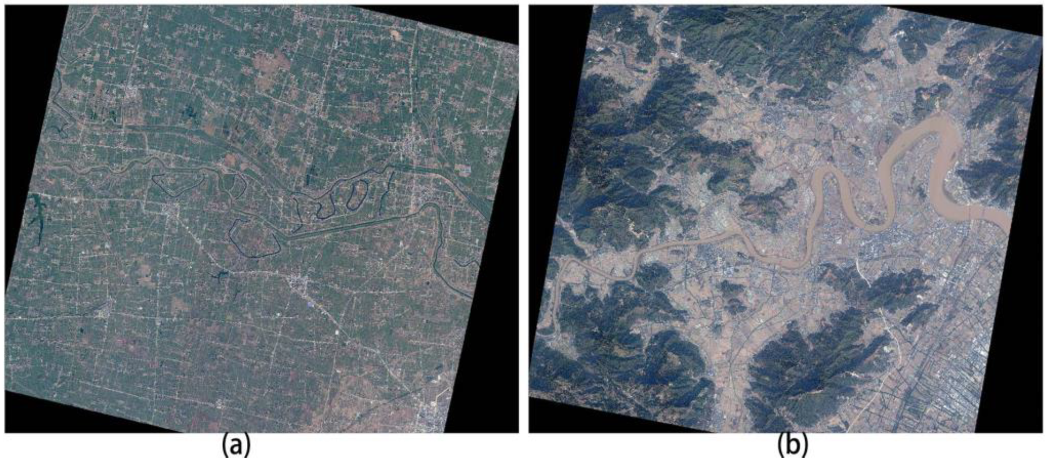
3.3. Experimental Data

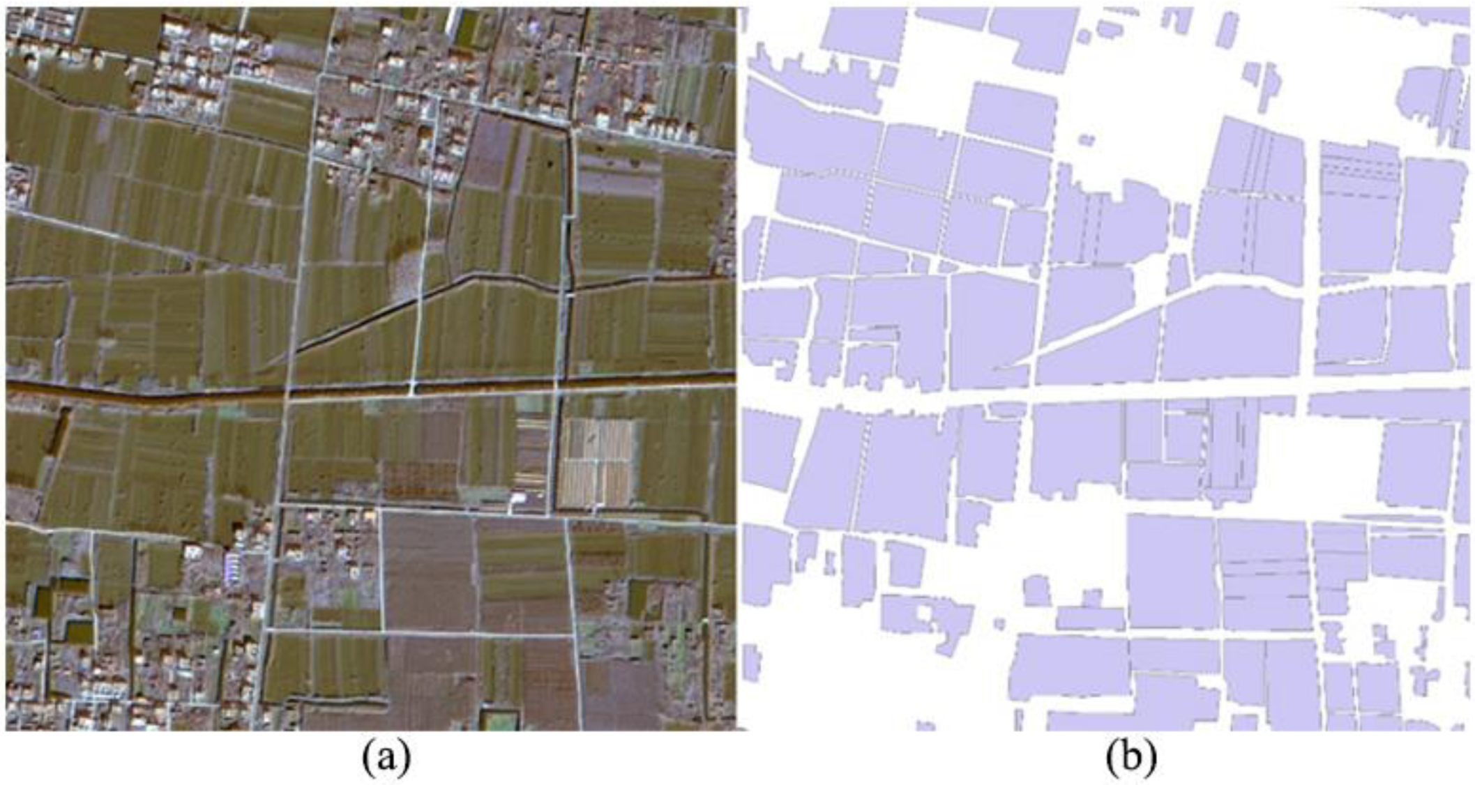
3.3.1. Data Labeling

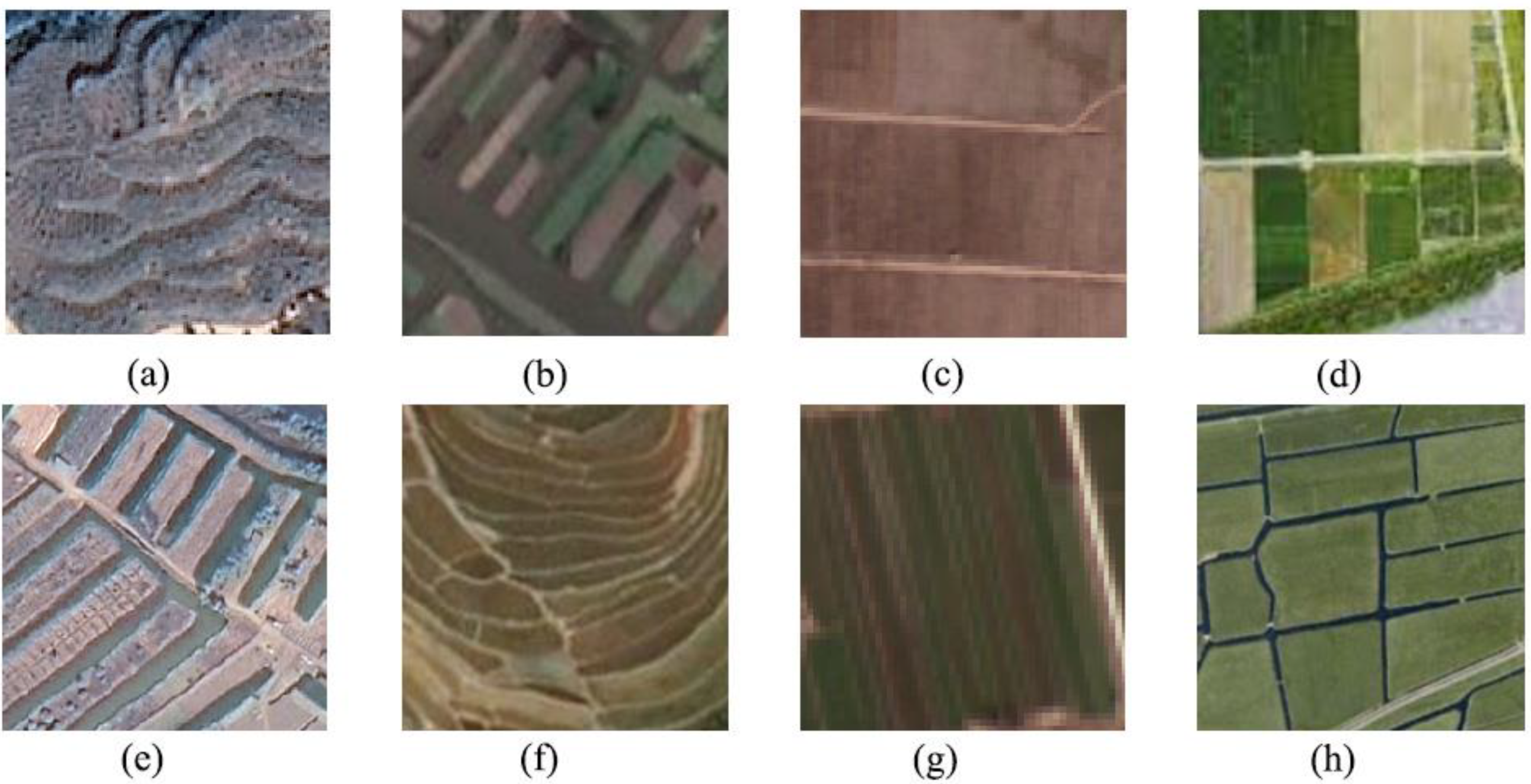
China has a vast territory and abundant resources, spanning 62 degrees and five time zones from east to west. China almost includes all terrains, including mountains, plateaus, hills, basins, plains, and deserts. In the long history of Chinese farmers gradually adapting to the geographical environment and living in harmony with it, spring plowing and autumn harvest have continued to this day. They have developed complex and diverse forms of arable land. In addition, with the continuous expansion of China’s population, the agricultural production mode has also shifted from extensive management to intensive management. The intensive farming agricultural production model is widely used to improve labor productivity per unit of land. This further leads to the concentration and density of agricultural cultivated land distribution. The diverse forms and distribution of arable land mean that the work of land parcel labeling is complex and extensive. For remote sensing land parcel image training data, there are significant differences between different land parcel types with the same semantic attribute, such as terraced fields and dry lands, terraced fields, and stacked fields. In addition, all kinds of plots exist in plains, mudflat, mountain slopes, and coastal tidal areas and are distributed intensively and widely. Even in the same remote sensing image, the vastly different planting environments, scattered and irregular distribution, alternating crop types, and the concealment of similar features in adjacent plots all bring difficulties for manual recognition. Therefore, it is necessary to organize and summarize typical plot types within the study area before manual annotation. The plot type is shown in Figure 1.

The basic characteristics of each type of land parcel are described as follows:

(a)

Dam field: A farmland formed by building a dam in a ravine to block soil washed down from the mountain.

(b)

Stacked fields: In the low-lying areas with dense river networks in southern China, farmers excavate soil from rivers and canals to adapt to seasonal floods and rising water levels and use it to build stacked high fields. Its high terrain and good drainage make it easy for crop irrigation, which is conducive to planting various dry land crops, especially suitable for the production of fruits and vegetables.

(c)

Dry land: This refers to a field that relies on natural precipitation for irrigation and does not hold water on its surface. Most plants are drought tolerant, such as wheat, cotton, and corn.

(d)

Paddy field: This refers to flooded farmland. Mainly concentrated in plain and basin hilly areas, with flat terrain and deep soil layers, it is suitable for planting semi aquatic crops such as rice and taro.

(e)

Taitian: A farmland formed as a platform above the ground and surrounded by ditches. The purpose is to eliminate waterlogging and improve alkaline land. It is beneficial for planting crops such as cotton, vegetables, and grain, and is a product of effective utilization of arable land resources in barren areas.

(f)

Terrace: A stepped cultivated land that slopes downwards at a certain slope. This type of land can effectively utilize the arable land resources of slopes and hills, making it easy to cultivate crops such as rice and wheat.

(g)

Striped fields: Fields surrounded by agricultural ditches and windbreak forests. Their land utilization rate is high, making it easy for machine farming and irrigation.

(h)

Dike field: Waterfront farmland formed by farmers building embankments along the river, near the sea, or by the lake for reclamation. It is an effective farming method for transforming lowlands and fully utilizing land resources.

Image datasets are the foundation of deep learning, and high-quality datasets help neural networks to understand the common features of segmented targets more completely and efficiently. So far, most publicly available remote sensing datasets have been constructed for road traffic, buildings, or natural scenes, and very few semantic segmentation datasets have been constructed for agricultural plots. Therefore, this paper selects two representative agricultural production areas in Anhui and Zhejiang as the study area and then collects high-resolution agricultural remote sensing satellite images with research significance in the region to construct a dataset.

Different satellites have different usage scenarios and characteristics. The data in this article are sourced from the Gaofen-2(GF-2) satellite [25] as shown in Figure 2. This is the first civilian optical remote sensing satellite independently developed by China with a spatial resolution better than 1 m. It is equipped with 0.8 m panchromatic and 3.2 m multispectral cameras and has characteristics such as sub-meter-level spatial resolution, high positioning accuracy, and fast attitude maneuverability. The specific characteristics are shown in

Table 1. Key parameters of the Gaofen-2 satellite.

Sensor	Band Number	Wavelength Range	Spatial Resolution	Width
Panchromatic	1	0.45–0.90 μm	0.8 m	45 km
Multispectral	2	0.45–0.52 μm	3.2 m
	3	0.52–0.59 μm	3.2 m
	4	0.63–0.69 μm	3.2 m
	5	0.77–0.89 μm	3.2 m

.

The excellent performance of the GF-2 satellite has effectively improved the comprehensive observation efficiency of the satellite, making its remote sensing image acquisition quality reach an internationally advanced level. Within the same agricultural production area, the GF-2 satellite can obtain images of both high and low resolutions. Therefore, this article can use high- and low-resolution images from the same region to create a dataset. Similarly, thanks to the multi-channel image acquisition capability of the GF-2 satellite, different channel combinations can be used to highlight land features during annotation, improving the efficiency and accuracy of dataset annotation work.

To efficiently label images in the same space at different times and in different bands, the geographic coordinate system of the ArcGIS software can be used to interpret and mark farm plots manually visually and save them as vector graphics [26].

The annotation work of the remote sensing land dataset in this article requires the manual classification of all land pixels in the image, one by one, and defining them as a basic land unit by circling the edges. Commonly used image annotation software includes LabelImg and Labelme. These kinds of annotation software belong to the type of first cropping and then annotating. They usually need, first, to cut the complete remote sensing image into 512 × 512 sized images for individual annotation and generate a corresponding label file to save after each annotation. They will generate a corresponding label file after each annotation and save it. This annotation method is usually suitable for situations where each small image contains complete target content, such as handwritten numbers, plant leaves, or transportation vehicles. The target content in these images is displayed completely in a single image. After annotation, the annotation content on each small image is also complete. The annotation of large-scale remote sensing images in such annotation software requires a method of first cutting and then annotating. This will inevitably lead to a single large plot being split, labeled, and saved in multiple small images, resulting in the inevitable edge errors that accumulate as the number of annotations increases. If you choose to directly annotate the large-sized image first and then crop the dataset, you can avoid this error and reduce the workload to a certain extent.

Using ArcGIS as the annotation software in this article can avoid the edge errors caused by cropping before annotation. As a professional geographic information processing software, ArcGIS can fully annotate remote sensing images and generate corresponding rasterization labels as a whole. Due to the fact that the annotation object is a complete geographical image within the target area, using a holistic annotation method can scale according to the size and distribution of the target plot during the annotation process. It is convenient to improve the accuracy of labeling the edges of the land parcel and to improve the accuracy of labeling by referring to the characteristics of the surrounding environment of the target land parcel.

First, the original remote sensing image to be processed is opened in ArcGIS and scaled to an appropriate scale for labeling; then, a *.shp vector layer is created as a marker mask and set as a face element to make it easier to outline the shape of the plot. Benefiting from ArcGIS’s ability to analyze geolocation information from remote sensing images, it is possible to set the projection coordinate system for remote sensing images according to the actual geolocation information collected by the satellite. For instance, the remote sensing image of Anhui Province can be set as WGS_1984_UTM_Zone_50N. Once set up, the plot vector labels can be fixed in an absolute position in the projection coordinate system. By fixing the original remote sensing image in the same approach, the coordinates of the original image and the label can be fixed relative to each other.

After setting the projection coordinates, the vector label layer is opened as a mask. Next, the plot is found according to the geographic features of the original map, and ArcGIS’s editing tools are adopted to outline the edges of the plot in the form of curves. These edges are saved when the outlined vector polygon fits the original plot perfectly.

To improve annotation accuracy and efficiency, the multi-channel information of remote sensing images can be reasonably used for plot annotation. By combining different bands in a specific arrangement, certain features can be highlighted, and the discrimination of specific features in the image can be improved as shown in

Table 2. The characteristics of remote sensing images in different wavebands.

Band No.	Band	Wave Length (μm)	Highlighting Features
Band1	Blue	0.45–0.52	Water bodies, soils, and vegetation
Band2	Green	0.52–0.59	Vegetation and trees
Band3	Red	0.63–0.69	Easy to observe bare ground and plant density
Band4	Near-infrared	0.77–0.89	Estimate biomass and distinguish paths

.

The focus of this article is the plot, which mainly consists of bare plots, plots that have already been shown, plots in the fallow period, and irregular plots such as terraces and pallets. To highlight the features of the plots, the near-infrared, red, and green bands are combined into a standard false-color image; plots with vegetation cover are shown in red, similar features such as ponds and open spaces are shown in blue, and plots without vegetation cover are shown in light grey. Visual sensitivity can be enhanced by highlighting target information and excluding distractions from similar features.

Once the labeling work is complete, the vector graphics are assigned farmland attribute values and rasterized, and finally, the entire image is cropped row by row and column by column with an overlap ratio of 0.1. Afterward, a 512 × 512 binary label file suitable for training is generated as shown in Figure 3.

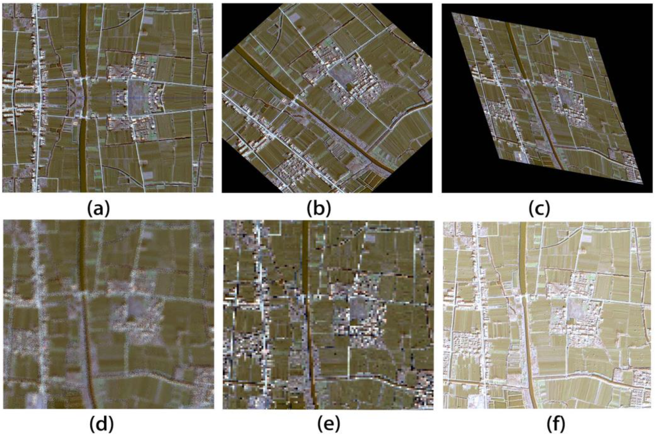
3.3.2. Data Augmentation

If the shape and texture of the image are complex and the amount of data is not sufficient, the network model generated in training will not reflect the common features between the plots well. Therefore, to expand the dataset and improve the generalization ability of the model, the existing dataset is pre-processed as shown in Figure 4.

In the figure, (a–f) show the effect of data enhancement, which is implemented as follows. (a) Horizontal mirroring: the top half of the original drawing is mirrored along the horizontal axis so that the bottom half of the image is replaced by the top half. (b) Center rotation: the original drawing is rotated 45° clockwise around its center to produce the rotated drawing. In practice, the resulting size will be partially outside the original frame. (c) Imitation transformations: a coordinate system is set up for the original figure to linearly transform and translate the coordinates of each pixel. The essence of the transformation is to multiply the original figure by a matrix and then add a vector; after the transformation, the lines in the figure remain straight, and the relative position of the lines remains unchanged. (d) Fuzzy processing: a random number is generated, the original pixel points are read row by row and column by column, and the pixel values around the point are extracted by filling the new image blur matrix with a random number. After traversing all the pixels in the original image, a new post-blur image is created. (e) Mosaic treatment: all the pixels in the original image are divided into small 4 × 4 blocks, then all 16 pixel values are changed to the value of the first pixel in the upper left corner of the block. The mosaic effect can be achieved by modifying small blocks of pixels in the full image one by one. (f) Brightness enhancement: brightness enhancement can be achieved by increasing the RGB value of each pixel in the original image by a suitable proportion.

4. Improved TransUNet Network Remote Sensing Plot Segmentation Experiment

To further improve the performance of remote sensing plot segmentation based on CNNs, the TransUNet network with the best segmentation results in the segmentation experiments is selected as the research object. The key structures of the TransUNet network, namely, the residual module and the jump connection, are analyzed and improved.

Overall, the improved network structure still adopts the classic U-shaped symmetrical structure, with the encoder section on the left, the decoder section on the right, and a jump connection in the middle to provide upsampling cascade data as shown in Figure 5.

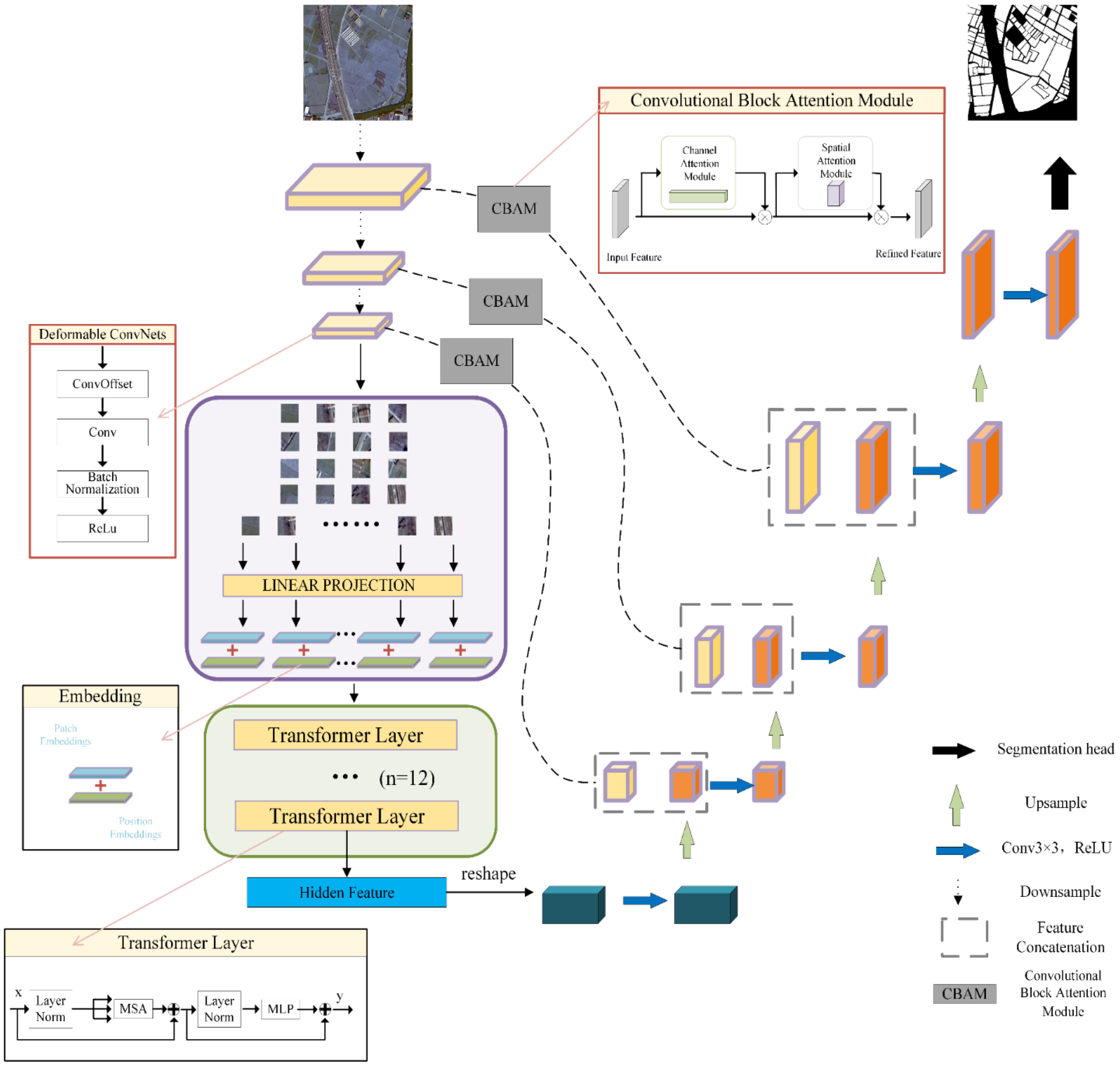
4.1. Residual Module Improvements

The encoder module uses the classical ResNet network framework for feature extraction. The ResNet framework is an outstanding CNN network proposed by Kai Ming He’s [27] team at Microsoft Asia Research in 2015, and it won first place in the ILSVRC and COCO competition. To improve the performance of CNNs, the ResNet network innovatively proposes a residual structure, which enables the neural network to not rely entirely on the overall mapping in the learning process, to directly refer to the residual results of the previous layer for learning where redundancy is too high, and to solve the gradient disappearance problem that occurs as the network deepens.

Depending on the depth of the network, the ResNet networks can be divided into different derivatives of ResNet18, ResNet34, ResNet50, ResNet101, and ResNet152. The deeper the network, the more complex the structure, and the greater the number of operational parameters. Considering that increasing the number of layers of the network can bring better learning results, and that reducing the computation amount can improve training efficiency and reduce time consumption, this paper still uses ResNet50 as the backbone of the original TransUNet network. Meanwhile, to better extract the features of plots with different scales and very different shapes in remote sensing images and to alleviate the problem of adhesive patches between different plots, Deformable ConvNets [28] is introduced to improve the original ResNet50 feature extraction network.

The most distinctive features of deformable convolution are its offset convolution layer and variable receptive fields. The offset learned by the offset convolution layer allows the position of the convolution sampling points to be adjusted accordingly, thereby providing the receptive field the ability to adapt to the scaling of the extracted target shape. This type of convolutional sampling point differs from the traditional regularly arranged rectangular sampling points in that it can change according to the content of the target image. The offsets generated by active learning can be calculated to change the shape and size of the receptive field according to the scale of the target plot, the shape of the edges, and other features. Thus, nine residual blocks in the last convolutional layer of the ResNet50 feature extraction network are improved by modifying all the 3 × 3 convolutions in the residual blocks to 3 × 3 deformable convolutions. Being able to adjust the sampling points of the deformable convolution, the feature extraction network can focus more on the target area and reduce the collection of features from irrelevant areas, further improving the network’s ability to extract plots in small crevices and complex terrains.

4.2. Jump Connection Improvements

After continuously extracting low-level features by the encoder convolution operation, embedding and labeling feature information by the embedding layer, as well as capturing global information context by the transformer coding layer, the feature extraction network has fully captured the feature information of the remotely sensing plot images. To restore this abstract feature information more fully to the input image dimensions, the decoder cascades the low-level feature information output from the encoder feature extraction process when performing the upsampling operation.

This type of connection is called a jump connection. To combine texture information with abstract features and improve the network’s ability to extract features from the plot, the original network uses three jump connections. However, the jump connections in the original network are a simple copy and paste of the feature information, and no further processing of the feature information is conducted. Therefore, this section computes and improves the jump–join step in conjunction with the convolutional block attention module (CBAM) [29] so that the cascade information output from this step can better represent the important target features and suppresses other background feature information.

The CBAM is a lightweight attention module and has little effect on the number of training parameters. However, it combines the channel attention module (CAM) and the spatial attention module (SAM) to adjust the weighting of the effective semantic and positional information of the target region with less computational overhead and a small number of additional parameters. This enables the jump connection step to output a more comprehensive feature map with more important details.

Therefore, the improved network proposed in this paper embeds a convolutional attention module on top of the original three-jump connection, and it performs channel attention and spatial attention on the feature information extracted from the encoder part, in turn. This can further improve the segmentation network’s ability to focus on the target plot features and reduce the interference of background features such as ponds and woods on the target plot. The feature information processed by the convolutional attention module is eventually used in the decoder to recover the image, enabling the network to cascade more deep and shallow feature information comprehensively.

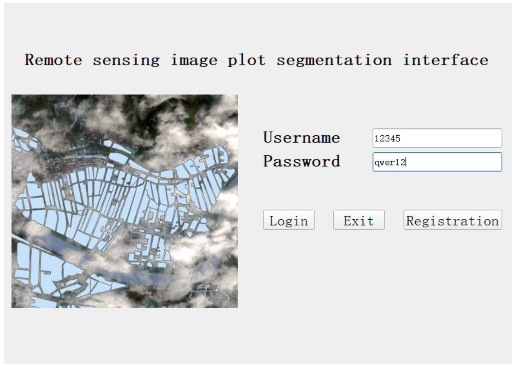
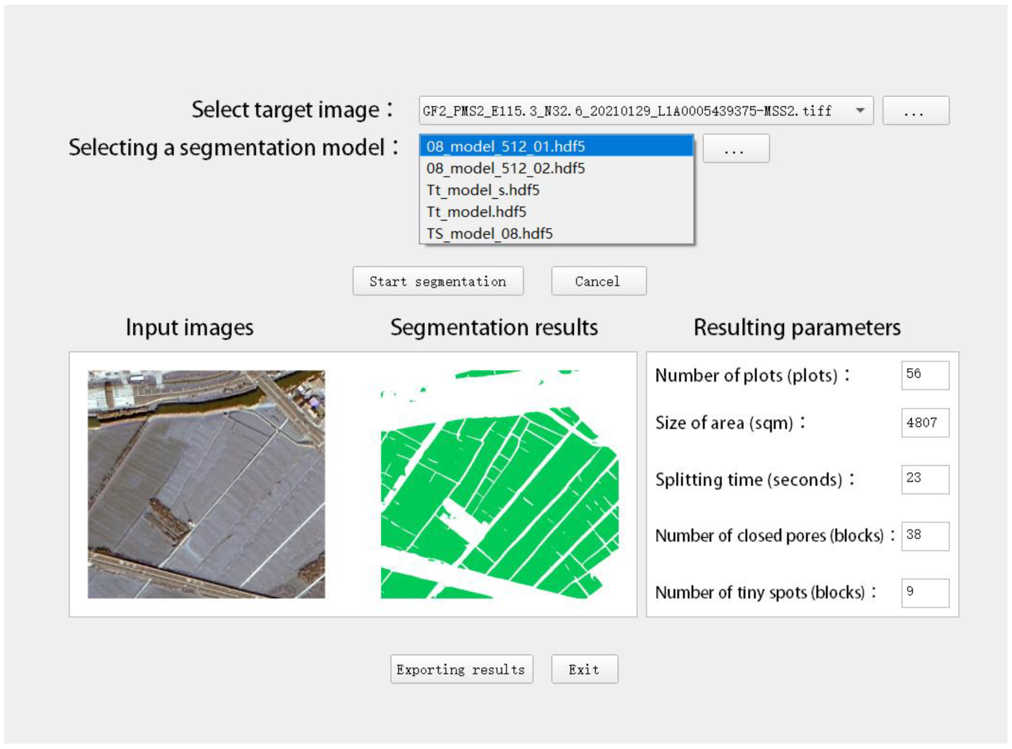
4.3. High-Resolution Remote Sensing Image Land Segmentation Software

To facilitate the use of the trained neural network model for plot segmentation of the acquired remote sensing images, this section uses PyQt5 to build a UI interface [30] to call a Python program for human–computer interaction in the segmentation process.

4.3.1. Development Environment

The operating system is Windows 10, the development tools are PyCharm, Python, and PyQt5. The QtWidgets module is used to create the main windows, the QtCore module handles file directories, and the QtGui module handles fonts and images, etc.

4.3.2. Interface Design

The segmentation interface design process includes the reading and presentation of the target image, as well as the presentation and saving of the segmentation results. The login screen provides different permissions for different users for plot splitting, exporting data, and viewing data only. Users can access the segmentation screen by entering the corresponding user name and password as shown in Figure 6.

In addition to the login and logout buttons, the login screen also provides a registration window for new users and assigns different rights to different users. Once you have followed the text instructions to register you can jump back to the login screen, enter the correct user name and password in the login screen to jump directly to the Remote Sensing Plot Segmentation page to perform plot segmentation on high-resolution remote sensing images.

Select the target image, enter this image address into the Python segmentation code, and then select the trained neural network model for plot segmentation. Finally, as shown in Figure 7, the segmentation result is output and displayed on the segmentation page. In the figure, the original image of the target remote sensing image is displayed in the left pane, and the segmentation result predicted by the current neural network model is displayed in the right pane. The output result is in a raster map format by default.

The Export button allows users to choose whether to save the target result image as a raster image or as a vector result. If the result is saved as a raster image, the result file path is opened directly in the segmentation code for manipulation. Selecting the format of the vectored result will call the GDAL library to vectorize the current raster image result before saving it.

5. Results

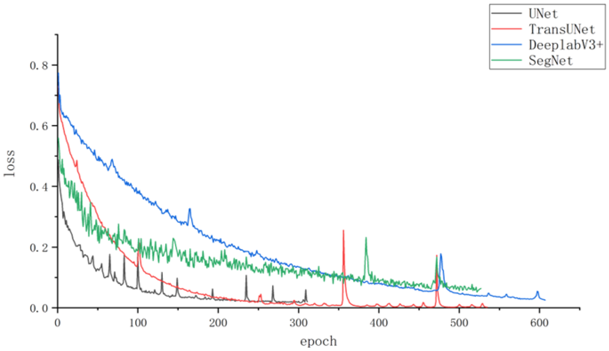
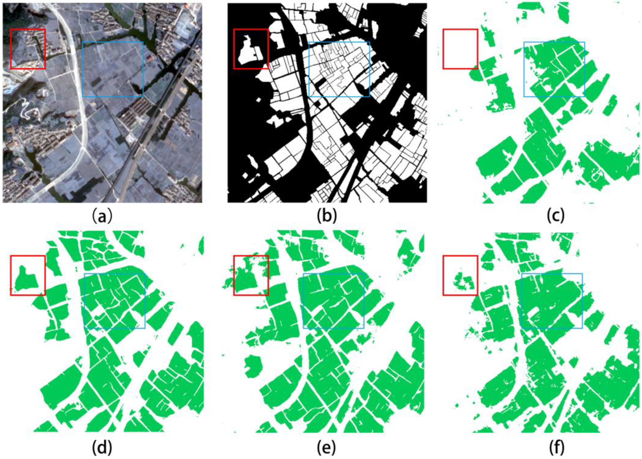
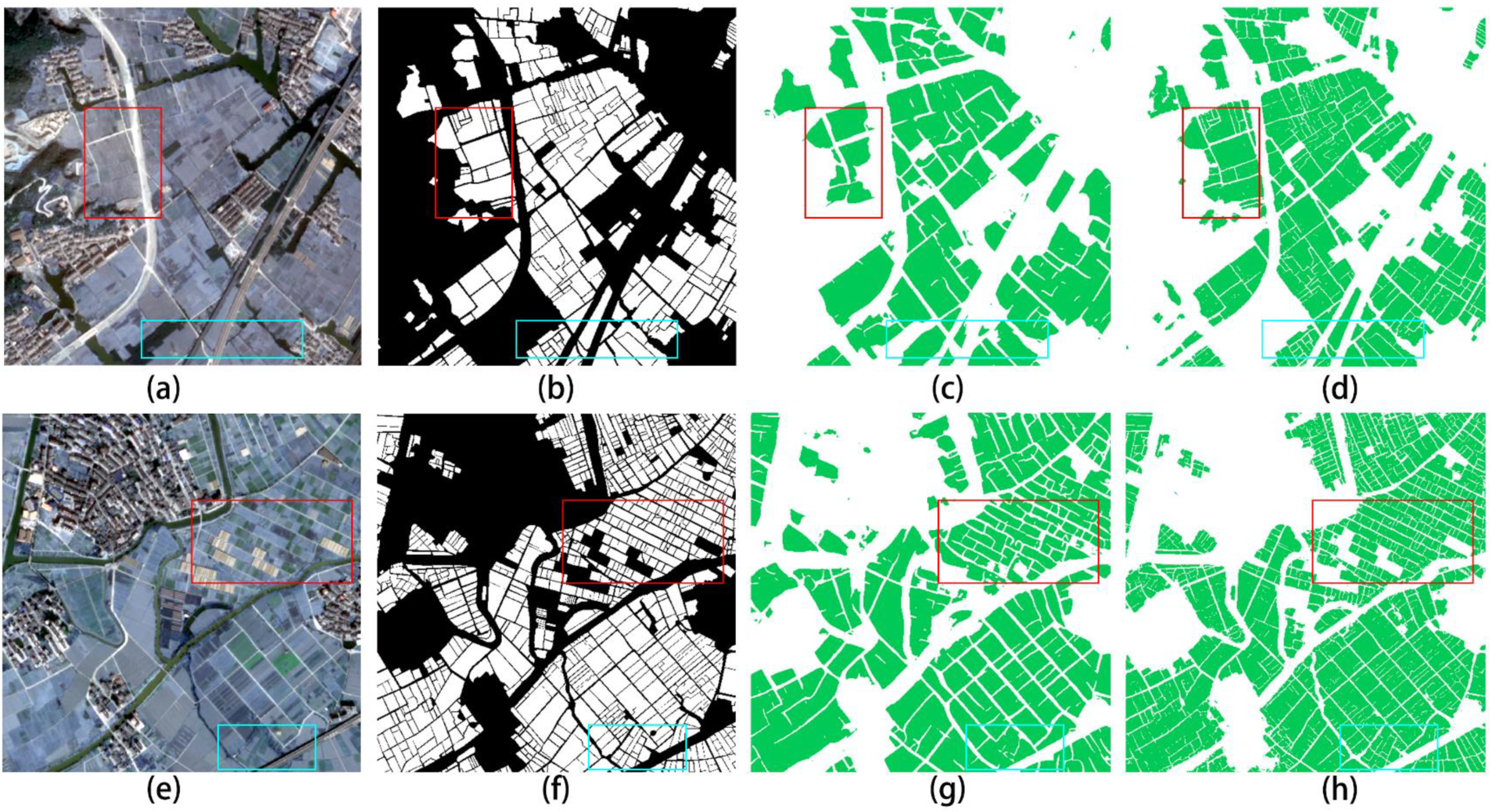
5.1. Mainstream Neural Network Remote Sensing Plot Segmentation Experiments Results

Using the data enhancement method can increase the amount of training data, prevent over-fitting of the training model, and improve the generalization ability of the trained model without providing new data samples.

The dataset used in this section is derived from remote sensing images of Zhejiang Province and Anhui Province with a resolution of 0.8 m, and it contains remote sensing images of various typical dam fields, drylands, and paddy fields in China. After eliminating the image data with no training value, a total of 7366 images were used for training as shown in

Table 3. The datasets used in the experiments.

Source	Training Set	Validation Set	Test Set	Total by Location	Total
Zhejiang Province	2550	737	368	3655	5136
Anhui Province	2586	750	375	3711

.

After configuring the training environment and training parameters, the four convolutional neural networks mentioned above, including SegNet, UNet, DeeplabV3+, and TransUNet, were built for training. The learning rate is adjusted automatically according to the current loss value during the experiment. In the training process, the validation loss value is checked every three epochs, and if it does not drop, the learning rate is adjusted to 80% of the current one. If the loss value does not drop for 30 consecutive rounds, the training process is completed, and the current model is retained as shown in Figure 8.

The initial batch size was set to four, the epoch was set to 500, the initial learning rate was set to $1\times {10}^{-4}$, and training was performed using a homemade remote sensing plot dataset with a resolution of 0.8 m.

The figure shows that the loss functions of the four CNNs converged as the training epoch gradually increased, and the training performance of each network differed.

To visually evaluate the segmentation effect of each network, Figure 9 shows the semantic segmentation results of the four networks for the same region of remote sensing images presented for comparison.

In the figure, (a) shows the remote sensing image of the plot, (b) shows the corresponding tag image, and these two images are taken as the evaluation criteria. (c) shows the segmentation results obtained by SegNet, from which it can be seen that the SegNet network can segment the overall distribution of plots, but fine plots and larger plots near the image edges are not correctly segmented. The fine plots near the mountain in the red box are not correctly divided, nor are the plots lines in the blue box. (d) shows the segmentation results of the TransUNet network, from which it can be seen that the TransUNet network has a better ability to capture details than the SegNet network. The fine plots in the red box are correctly segmented, and the fine plots in the outer part of the box are also well represented. Compared to SegNet, TransUNet identified significantly more plots correctly. Meanwhile, the number of divisions of the fine plots in the blue box is also higher. (e) shows the segmentation results of a plot by the UNet, and it performs similarly to TransUNet. However, its segmentation of local fine plots is slightly worse, and there are obviously mis-segmented plots. The fine plots in the red box that follow the hills are correctly segmented, but the green vegetation on the nearby hills is incorrectly segmented into plots. The segmentation of the tiny plots in the blue boxes is also represented, which is similar to the segmentation result of the TransUNet network. However, there are several places on the map where mountains and lakes are incorrectly segmented as cropland, which affects the overall segmentation results. Finally, the segmentation results of the DeeplabV3+ network are shown in (f). The tiny plots in the red boxes are identified but not segmented with the correct contours. The edges of the segmentation results in the blue boxes are messy and poorly connected. Overall, DeeplabV3+ has an inferior ability to segment plot details to TransUNet and UNet with U-shaped structures.

Overall, the TransUNet network performed better in terms of detail than the SegNet and DeeplabV3+ networks, and it correctly segmented more concrete pavement and houses between plots. Also, it segmented most large plots correctly, with fewer areas of plots being incorrectly segmented. Moreover, TransUNet is better at segmenting the ridges between plots than UNet and the other two networks, and the resulting plots have more regular edges in the segmentation maps. The number of mis-segmented trivial plots and the number of pores within plots were also significantly lower than those of the other networks. So, the TransUNet network outperformed the other three networks in the remote sensing plot segmentation experiment on the dataset constructed in this paper.

To compare the segmentation performance of different networks in more detail, parameters such as pixel accuracy and IoU were calculated separately for analysis.

It can be seen from

Table 4. Evaluation of the prediction results of the four networks.

Methods	PA (%)	Recall (%)	F1-S (%)	IoU (%)
SegNet	77.07	80.56	65.29	48.47
TransUNet	86.07	83.56	81.94	69.41
UNet	83.22	76.42	79.50	65.98
DeeplabV3+	80.65	84.04	71.79	56.00

that the comparison results and the visualization of the segmentation results are consistent. The SegNet network achieves the lowest accuracy rate, which is 9% less than the TransUNet network and 6.15% less than the UNet network, indicating that the area of cultivated land not identified as plots in the segmentation results of the SegNet network is larger and the area of incorrectly identified plots is larger than that of TransUNet and UNet. The pixel accuracy of the UNet and TransUNet networks is high, and the results are relatively close at 83.22% and 86.07%, respectively. This indicates that both have better performance in terms of overall plot segmentation accuracy.

To sum up, the TransUNet network is slightly better than the other networks in terms of PA, IoU, and F1-score. Compared to the UNet network, which is the best-performing among the other three networks, the accuracy is 2.85% higher, the F1-score is 2.44% higher, and the IoU is 3.43% higher. It demonstrates that the TransUNet network trained with the dataset constructed in this paper performs better in the semantic segmentation of remote sensing image plots, and it shows fewer recognition errors and more correct detail segmentation.

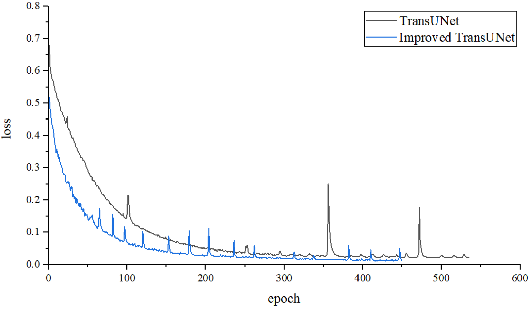
5.2. Improved TransUNet Network Remote Sensing Plot Segmentation Experiment Results

As shown in Figure 10, the TransUNet and modified TransUNet networks were constructed separately, and the experimental environment, experimental dataset, and evaluation metrics consistent with the previous segmentation comparison experiments were used for training and analysis.

The change in the loss value shows that the improved network converges faster and can reduce the loss value to within 0.1 in a shorter period. Meanwhile, the improved network has less fluctuation in the overall loss value decrease process, and no significant fluctuation occurs. This indicates that the improved network is more stable and faster than the original network in terms of gradient descent.

In Figure 11, (a,b) and (e,f) show the original remotely sensing images of the farmland plots and the corresponding labeled images, respectively. (c,g) and (d,h) correspond to the segmentation results of the TransUNet network and its modified network. It can be seen from the segmentation results (c,d) before and after the improvement in the first row that the improved network has more detail in the segmentation results, and the number of correctly segmented plots has improved. The narrow rows of monopolies and roads between the plots in the red box in (d) are more specifically segmented than those in (c). The strip of plots next to the highway in the blue box in (d) is also more complete than the resultant split in (c). Therefore, compared to the original network, the improved network allows a more complete and correct segmentation of plots.

The segmentation results in (g,h) obtained by the TransUNet network before and after optimization indicate that the thin field ridges in the blue boxes in both plots are only correctly segmented by the improved network, rather than being presented as gaps in plot (g). As for the segmentation result in (h) obtained by the improved network, the factory shed in the red box is not incorrectly segmented into plots as in (g). This indicates that the correctness of the segmentation result of the improved algorithm has been enhanced compared with that of the original algorithm.

Comparing the segmentation results of the improved network with the original map labels reveals some defects. First, some of the green vegetation close to the residential buildings in the original plan (a) is incorrectly divided into plots in plan (d). Second, in the original map (h), there are also small blocks of residential buildings that are split into plots by the improved network. Third, there is still a gap between the improved network segmentation results and the original map labels in terms of the clarity of the row monopoly and road segmentation between the plots.

Overall, the improved network can segment plots in greater detail than the original network, with a smaller area of error segmentation. Nevertheless, for error-prone feature targets such as green bushes and green ponds, there are still subtle errors in the segmentation results of the improved network, and the level of detail in the segmentation of plots, rows of monopolies, and roads can be further increased.

By comparing the evaluation parameters such as pixel accuracy and intersection ratio, the differences between the original and the improved algorithms can be specifically analyzed.

It can be found from

Table 5. Segmentation results of the TransUNet network and the improved TransUNet network.

Methods	PA (%)	Recall (%)	F1-S (%)	IoU (%)
TransUNet	86.07	83.56	81.94	69.41
Improvements to TransUNet	92.39	91.41	92.63	86.28

that the improved TransUNet network obtains more accurate prediction results than the original network. In the prediction results for the dataset in this paper, the segmentation results of the improved network show a 6.32% increase in PA and a 7.85% increase in Recall. This indicates that the improved network correctly segmented the plots while also ensuring the accurate identification of other features, thereby reducing the number of non-plot features that were incorrectly segmented as plots. The most significant improvement in the evaluation metric was the F1-score, which improved by 10.69%. This further demonstrates that the improved TransUNet network has fewer errors in plot segmentation of remote sensing images, and the segmented plot area is closer to the actual annotated area. These results show that the improved network performs better in segmenting the dataset established in this paper and can segment the plot targets in remote sensing images more accurately and effectively.

Through ablation experiments, the robustness of the model can be verified after removing certain specific parts. This is crucial for confirming whether the model is overly dependent on certain features or structure, and it can determine which components contribute the most to model performance, providing guidance for model improvement. This helps to optimize the model structure, improving its efficiency and performance. When deep learning models become too complex, ablation experiments can help simplify the model, remove unnecessary parts, and improve the interpretability and manageability of the model.

5.3. Ablation Experiments

In order to verify the effectiveness of Deformable ConvNets and CBAM, ablation experiments were conducted on datasets in Zhejiang. On the basis of the improved TransUNet network, we remove Deformable ConvNets and CBAM, respectively. The results of the experiments are shown in Figure 12.

In Figure 12, ‘Remove CBAM’ refers to TransUNet with residual module improvement. ‘Remove Deformable Convnets’ refers to TransUNet with jump connection improvement. The improved TransUNet reaches a good accuracy of 92.39%. TransUNet networks with residual module improvement and jump connection improvement, respectively, reach an accuracy of 92.06% and 91.81%. The results of experiments indicate that adding Deformable ConvNets and CBAM to TransUNet network improves the performance of network recognition.

6. Discussion

Compared to traditional land parcel segmentation methods and existing segmentation methods based on convolutional neural networks, the remote sensing land parcel segmentation method proposed in this paper has higher accuracy and stronger practicality. Overall, it involves collecting cultivated land images captured by GF-2 remote sensing satellite and establishing a dataset, conducting experiments to evaluate the performance of mainstream neural networks in land segmentation, constructing and improving TransUNet neural networks for segmentation experiments, and optimizing low-resolution segmentation results by combining vectorization post-processing technology.

This paper uses typical farmland image data collected by the Gaofen-2 satellite to create a dataset. The data source is relatively unique, and the number of farmlands with various characteristics is uneven. The proportion of uncommon farmland such as terraced fields, polder fields, and stacked fields is relatively small. Additional data sources should be added, and more remote sensing images of farmland from different regions should be collected as basic data. Adding remote sensing images collected by QuickBird satellite for dataset production will effectively improve data diversity.

Also, the length of shadows cast by buildings under different lighting environments varies over time, resulting in significant differences in the characteristics of land parcels near buildings under shadow cover. For areas with significant variations in such differences, such as land parcels with shadow coverage, tidal changes, and cloud cover, efforts should be made to collect remote sensing images from different time periods to enrich training data or to optimize algorithms for such image features.

The block segmentation results based on low-resolution data have rough edges and numerous internal pores. The reason may be poor clarity of low-resolution images and the large jagged edges of the images. Adopting appropriate preprocessing methods on the original image before segmentation may further improve the segmentation effect and broaden the application scenarios to enhance image quality.

In addition, based on this, a vectorization post-processing step can be designed to remove fine patches from the low-resolution segmentation results, fill the pores inside the plot, and smooth the edges of the plot. This approach saves a significant amount of time, computing power, and data costs. Thanks to the vector map results output by this method, not only does the data occupy less space, making it easy to efficiently call and analyze in geographic information software, but it can also be reused on remote sensing images obtained at other times in the same region or at other resolutions.

7. Conclusions

Until now, remote sensing has been the only means of providing dynamic observational data on a global scale, characterized by spatial continuity, repeatability, and time series. However, the image information is complex and massive. It is a difficult and time-consuming to process data, and it is hard to guarantee efficiency and cost using manual recognition or machine learning methods.

This paper conducts training and segmentation experiments on high-resolution remote sensing plots with mainstream neural networks such as SegNet, UNet, DeepLabV3+, and TransUNet. The effectiveness and practical advantages of the TransUNet network in remote sensing plot segmentation are verified through a cross-sectional comparison of the practical remote sensing plot segmentation performance of different models. Based on this, the original TransUNet network is improved in terms of the residual module and the jump connection to enhance the semantic segmentation effect. Finally, experiments are carried out to compare and analyze the segmentation results of the improved network before and after optimization. The experimental results indicate that the TransUNet network with improved residual modules and jump connections can fully utilize the global information of the image while maintaining higher accuracy in detail processing. Segmentation result parameters for the improved TransUNet network have been comprehensively improved. It both reduces the number of other remotely sensed features that are incorrectly segmented as plots and increases the number of plots that are correctly segmented out, leading to higher overall segmentation performance.

Nevertheless, there are still shortcomings in this paper. The length of the shadows cast by buildings under different lighting environments varies over time, resulting in significant variations in the characteristics of land parcels near buildings under shadow cover. For areas with significant variations in such differences, such as land parcels with shadow coverage, tidal changes, and cloud cover, we should try to collect remote sensing images from different time periods to enrich training data or optimize algorithms for such image features.

References

1. Thenkabail, P.S. Global croplands and their importance for water and food security in the twenty-first century: Towards an ever green revolution that combines a second green revolution with a blue revolution. Remote Sens. 2010, 2, 2305–2312. [Google Scholar] [CrossRef]
2. Zhai, T.; Du, Q. Research on Augmented Reality Software Technology in Remote Sensing. Wirel. Internet Technol. 2017, 20, 52–53. [Google Scholar]
3. Li, Y.; Zhao, X.; Tan, S. Remote sensing monitoring of mine development environment based on high resolution Satellite imagery. J. Neijiang Norm. Univ. 2021, 36, 68–72. [Google Scholar]
4. Meng, J.; Wu, B.; Du, X.; Zhang, F.; Zhang, M.; Dong, T. Application progress and prospect of remote sensing in Precision agriculture. Remote Sens. Land Resour. 2011, 3, 1–7. [Google Scholar]
5. Atzberger, C. Advances in remote sensing of agriculture: Context description, existing operational monitoring systems and major information needs. Remote Sens. 2013, 5, 949–981. [Google Scholar]
6. Leo, O.; Lemoine, G. Land Parcel Identification Systems in the Frame of Regulation (ec) 1593, 2000 Version; Report; Publications Office of the European Union: Brussels, Belgium, 2000. [Google Scholar]
7. Guo, Z.; Chen, Y. Image thresholding algorithm. J. Commun. Univ. China (Nat. Sci. Ed.) 2008, 2, 77–82. [Google Scholar]
8. Duan, R.; Li, Q.; Li, Y. A review of image edge detection methods. Opt. Technol. 2005, 3, 415–419. [Google Scholar]
9. Li, H.; Guo, L.; Liu, H. Remote sensing image fusion method based on region segmentation. J. Photonics 2005, 12, 1901–1905. [Google Scholar]
10. Qi, L.; Chen, P.H.; Wang, D.; Chen, L.K.; Wang, W.; Dong, L. A ship target detection method based on SRM segmentation and hierarchical line segment features. J. Jiangsu Univ. Sci. Technol. (Nat. Sci. Ed.) 2020, 34, 34–40. [Google Scholar]
11. Qin, Y.; Ji, M. A semantic segmentation method for high-resolution remote sensing images combining scene classification data. Comput. Appl. Softw. 2020, 37, 126–129+134. [Google Scholar]
12. Shang, J.D.; Liu, Y.Q.; Gao, Q.D. Semantic segmentation of road scenes with multi-scale feature extraction. Comput. Appl. Softw. 2021, 38, 174–178. [Google Scholar]
13. Qi, L.; Li, B.Y.; Chen, L.K. Improved Faster R-CNN based ship target detection algorithm. China Shipbuild. 2020, 61 (Suppl. S1), 40–51. [Google Scholar] [CrossRef]
14. Chen, Y.; Jiang, H.; Li, C.; Jia, X.; Ghamisi, P. Deep feature extraction and classification of hyperspectral images based on convolutional neural networks. IEEE Trans. Geosci. Remote Sens. 2016, 54, 6232–6251. [Google Scholar]
15. Maggiori, E.; Tarabalka, Y.; Charpiat, G.; Alliez, P. Convolutional neural networks for large-scale remote-sensing image classification. IEEE Trans. Geosci. Remote Sens. 2016, 55, 645–657. [Google Scholar] [CrossRef]
16. Li, Y.; Xiao, C.; Zhang, H.; Li, X.; Chen, J. Semantic segmentation of remote sensing images by deep convolutional fusion of conditional random fields. Remote Sens. Land Resour. 2020, 32, 15–22. [Google Scholar]
17. Su, J.; Yang, L.; Jing, W. A semantic segmentation method for high-resolution remote sensing images based on U-Net. Comput. Eng. Appl. 2019, 55, 207–213. [Google Scholar]
18. Chen, T.H.; Zheng, S.Q.; Yu, J. Remote sensing image segmentation using improved DeepLab network. Meas. Control. Technol. 2018, 37, 34–39. [Google Scholar]
19. Chen, L.C.; Zhu, Y.; Papandreou, G.; Schroff, F.; Adam, H. Encoder-decoder with atrous separable convolution for semantic image segmentation. In Proceedings of the European conference on computer vision (ECCV), Munich, Germany, 8–14 September 2018; pp. 801–818. [Google Scholar]
20. Shelhamer, E.; Long, J.; Darrell, T. Fully convolutional networks for semantic segmentation. IEEE Trans. Pattern Anal. Mach. Intell. 2016, 39, 640–651. [Google Scholar] [CrossRef] [PubMed]
21. Badrinarayanan, V.; Kendall, A.; Cipolla, R. Segnet: A deep convolutional encoder-decoder architecture for image segmentation. IEEE Trans. Pattern Anal. Mach. Intell. 2017, 39, 2481–2495. [Google Scholar]
22. Yang, J.; Zhou, Z.; Du, Z.; Xu, Q.; Yin, H.; Liu, R. High resolution remote sensing image extraction of rural construction land based on SegNet semantic model. J. Agric. Eng. 2019, 35, 251–258. [Google Scholar]
23. Jiang, J.; Lyu, C.; Liu, S.; He, Y.; Hao, X. RWSNet: A semantic segmentation network based on SegNet combined with random walk for remote sensing. Int. J. Remote Sens. 2020, 41, 487–505. [Google Scholar] [CrossRef]
24. Ronneberger, O.; Fischer, P.; Brox, T. U-net: Convolutional networks for biomedical image segmentation. In Proceedings of the International Conference on Medical Image Computing and Computer-Assisted Intervention, Munich, Germany, 5–9 October 2015; Springer: Berlin/Heidelberg, Germany, 2015. [Google Scholar]
25. Pan, T. Technical characteristics of Gaofen-2 satellite. China Aerosp. 2015, 1, 3–9. [Google Scholar]
26. Wu, H.F. Research on the application of ARCGIS in the calculation and statistics of the area of land acquisition measurement. Sichuan Archit. 2022, 42, 73–75. [Google Scholar]
27. He, K.; Zhang, X.; Ren, S.; Sun, J. Deep Residual Learning for Image Recognition. Microsoft Res. 2015, 770–778. [Google Scholar] [CrossRef]
28. Dai, J.; Qi, H.; Xiong, Y.; Li, Y.; Zhang, G.; Hu, H.; Wei, Y. Deformable convolutional networks. In Proceedings of the IEEE International Conference on Computer Vision, Venice, Italy, 22–29 October 2017; pp. 764–773. [Google Scholar]
29. Woo, S.; Park, J.; Lee, J.Y.; Kweon, I.S. Cbam: Convolutional block attention module. In Proceedings of the European Conference on Computer Vision (ECCV), Munich, Germany, 8–14 September 2018; pp. 3–19. [Google Scholar]
30. Huang, R. AI image recognition tool based on PYQT5. Mod. Ind. Econ. Informatiz. 2023, 13, 90–91+94. [Google Scholar] [CrossRef]
Figure 1. Example of a remote sensing image of a typical plot of land. (ah) represent the dam field, stacked fields, dry land, paddy field, taitian, terrace, striped fields and dike field, respectively.
Remotesensing 16 00346 g001
Figure 2. Remote sensing images acquired by satellite. Both images above have a resolution of 0.8 m. (a) shows a 27,844 × 26,864 four-band remote sensing image of the farmland in Anhui Province, which can generate 3711 effective training images of 512 × 512 pixels. (b) shows a 27,500 × 26,760 four-band remote sensing image of the farmland in Zhejiang Province, which can generate 3655 effective training images.
Remotesensing 16 00346 g002
Figure 3. An example of a labeled and cropped original image and the corresponding label. (a) shows a cropped image of a remote sensing image of farmland in Anhui province, and (b) shows the plot labels at the corresponding locations. The purple part in (b) indicates farmland, and the white part indicates other features. After cropping the annotated images and corresponding labels to a suitable size for training, the entire dataset is divided into training, validation, and test datasets according to 7:2:1.
Remotesensing 16 00346 g003
Figure 4. Data pre-processing results. The methods of enhancement of (af) are horizontal mirroring, center rotation, imitation transformations, fuzzy processing, mosaic treatment and brightness enhancement, respectively.
Remotesensing 16 00346 g004
Figure 5. The structure of the improved TransUNet network.
Remotesensing 16 00346 g005
Figure 6. Login screen.
Remotesensing 16 00346 g006
Figure 7. The remote sensing image segmentation interface.
Remotesensing 16 00346 g007
Figure 8. Loss curves for the training of four types of neural networks.
Remotesensing 16 00346 g008
Figure 9. Plot of prediction results of four neural networks. (a) is a remote sensing image of the land parcel. (b) is the corresponding label image. (c) shows the segmentation results of SegNet network. (d) shows the segmentation results of the TransUNet network. (e) shows the segmentation results of UNet. (f) is the results of DeeplabV3+Network segmentation.
Remotesensing 16 00346 g009
Figure 10. The loss curve of the TransUNet network and the improved TransUNet network.
Remotesensing 16 00346 g010
Figure 11. Graph of segmentation results for TransUNet network and improved TransUNet network. (a,b,e,f) are the original remote sensing images and corresponding label images of farmland plots, respectively. (c,d,g,h) correspond to the segmentation results of the TransUNet network and its improved network.
Remotesensing 16 00346 g011
Figure 12. The ablation experiment’s results.
Remotesensing 16 00346 g012