Article

Examining the Dynamics of Vegetation in South Korea: An Integrated Analysis Using Remote Sensing and In Situ Data

1
Centre for Advanced Modelling and Geospatial Information Systems (CAMGIS), School of Civil & Environmental Engineering, Faculty of Engineering and IT, University of Technology Sydney, Sydney, NSW 2007, Australia
2
Earth Observation Centre, Institute of Climate Change, Universiti Kebangsaan Malaysia, Bangi 43600 UKM, Selangor, Malaysia
3
Ecological Information Team, National Institute of Ecology, 1210 Geumgang-ro, Maseo-myeon, Seocheon-gun 33657, Republic of Korea
*
Author to whom correspondence should be addressed.
Remote Sens. 2024, 16(2), 300; https://doi.org/10.3390/rs16020300
Submission received: 28 November 2023 / Revised: 2 January 2024 / Accepted: 9 January 2024 / Published: 11 January 2024

Abstract

:
Vegetation constitutes the primary component of terrestrial ecosystems and plays a crucial role in examining global climate change and its impacts. Assessing vegetation dynamics over significant periods of time can provide critical information on changes in vegetation cover and regional climate. Satellite-based remote sensing products offer a unique opportunity to analyze these changes at a country scale. South Korea has a unique history of forest regeneration, and studying this relationship provides an opportunity to examine its impact. To achieve this, we employ the vegetation–precipitation relationship using time series segmentation on residual trends (TSS-RESTREND), a statistical method that calculates the correlation between the annual maximum vegetation index and cumulative rainfall. This method helps identify time-step changes related to structural changes in the ecosystem. Using the enhanced vegetation index (EVI) and rainfall, this study aims to uncover the underlying dynamics and driving forces behind observed ecosystem changes, facilitating a deeper comprehension of the intricate interactions between vegetation and precipitation through the application of TSS-RESTREND. The findings increase knowledge of the complex relationship between vegetation growth and rainfall, given the country’s commendable forest regeneration program, even in the face of rapid urbanization. Moreover, the integration of finer resolution land cover images derived from in situ data not only provides a nuanced understanding of vegetation dynamics across diverse regions, but also underscores the critical need for continued collection of in situ data to provide more accurate and comprehensive analyses. The findings underline the pivotal role played by land resource management practices and underscores the significance of implementing adaptive conservation strategies, thereby contributing to the preservation of a stable and sustainable vegetation cover. The findings serve as a call for the ecosystem monitoring and strategic adaptation required to examine the environmental and ecosystem structural changes in the region. This study sheds light on the critical relationship between land management practices, environmental sustainability, and the resilience of the region’s vegetation amidst an ever-changing landscape.

1. Introduction

Vegetation plays a crucial role in maintaining the structural and functional integrity of terrestrial ecosystems on Earth. It is a key component in regulating the water cycle, energy exchange processes, and biogeochemical cycles that shape terrestrial surfaces [1,2,3]. Vegetation also plays a significant role in regulating terrestrial carbon cycles, providing ecosystem services, and influencing surface energy exchange and the water balance at both regional and global scales [4,5,6,7]. Alterations in vegetation patterns and dynamics can provide broad insight into the structural transformations occurring in a region. Vegetation changes are predominantly related to changes in climatic variables such as rainfall and temperature [8]. Examining vegetation dynamics is important for understanding vegetation–climate relationships at regional scales and to guide sustainable management and the conservation of natural resources [9].
Satellite-based remote sensing datasets provide a reliable and accurate means of examining vegetation dynamics and vegetation–climatic relationships [10]. Spectral vegetation indices are one of the most widely used forms of satellite data for evaluating [11] and monitoring vegetation cover [12], vegetation conditions [13], vegetation dynamics [14], and vegetation changes [15]. Long-term Moderate Resolution Imaging Spectroradiometer (MODIS) datasets provide consistent and long-term information related to vegetation characteristics. The two most used vegetation indices are the Normalized Difference Vegetation Index (NDVI) and the Enhanced Vegetation Index (EVI), widely accepted remote sensing metrics for monitoring vegetation growth and coverage change [10,12,15]. They utilize the sensitivity of vegetation to the red and near-infrared bands of the electromagnetic spectrum to provide an estimation of vegetation biomass and health. The NDVI is chlorophyll-sensitive, whereas the EVI is more responsive to canopy structural variations. The two vegetation indices complement each other in global/regional vegetation studies. The EVI was developed to optimize the vegetation signal with improved sensitivity in high biomass regions and improved vegetation monitoring through a de-coupling of the canopy background signal and a reduction in atmosphere influences.
Both the NDVI and EVI have been used for various purposes including monitoring long-term vegetation trends [16], studying vegetation dynamics [17,18], and identifying relationships between vegetation and climate factors [19]. For example, Bao et al. [16] studied vegetation responses to regional climate change between 1982 and 2010 on the Mongolian Plateau. Their trend analysis showed a shift in trends from the 1990s. Before the mid-to-late 1990s, an upward trend in the NDVI with a rise in rainfall and temperature was observed; however, after the mid-to-late 1990s, a reversal pattern was found with a decrease in rainfall. Lamchin et al. [20] studied the correlation between vegetation greenness and climatic variables for Asia using the Mann–Kendall test and found temperature to be a key variable in impacting vegetation greenness across the continent, including South Korea.
Research on vegetation dynamics utilizing satellite-based spectral indices often uses statistical techniques to understand various facets of vegetation changes. This study focuses on understanding the long-term vegetation trends and vegetation–climate relationships in South Korea at a country scale. Studying the country-scale vegetation patterns of South Korea is important for two reasons: (1) It has a long history of reforestation programmes beginning in 1973 and accelerating thereafter. The forest volume increased from 11.3 m3/ha in 1973 to 125.6 m3/ha in 2010 and 150.2 m3/ha in 2016 (Korea Forest Service 2017). This increase in forest volume had substantial co-benefits, such as a 43% rise in water yield and an 87% reduction in soil losses from 1971 to 2010 [21]. (2) Examining the relationship between climatic and land cover variables is essential for understanding their influence on different vegetation types. Climatic variables, including but not limited to rainfall, air temperature, land surface temperature (LST), and several others, can serve as a proxy to explain the variances exhibited by vegetation indices. For instance, Ukasha et al. [22] examined the relationship of the NDVI and Leaf Area Index (LAI) with hydroclimatic variables for two river basins in California. Their results suggested that the LAI was correlated with atmospheric demand for water, whereas the NDVI was correlated with water availability.
The most frequently used statistical approaches for assessing vegetation dynamics are correlation analysis [22], linear regression [23], the Breaks For Additive Season and Trend (BFAST) approach [24], the TIMESAT software package for time series processing and assessment of vegetation dynamics [25], the Mann–Kendall trend test [26], time series segmentation on residual trends (TSS-RESTREND) [27], wavelet transform analysis, and several others. Liu and Menzel [28] used a combination of the wavelet transform test, the Mann–Kendall trend test, and correlation analysis to examine the relationship between the NDVI and climatic variables in Southwest Germany. Ghebrezgabher et al. [23] used several statistical techniques including ordinary least squares, slope, linear regression, and correlation coefficients to study the relationship between climatic factors and the NDVI in the Horn of Africa. The advantage of using TSS-RESTREND over other trend methods is due to its utilization of residuals rather than actual values to calculate trends. The residuals result from the linear regression analysis between vegetation and climatic variables. Residuals remove the impact of climatic factors on vegetation change and detect more significant change pixels. Although numerous studies have examined vegetation trends at both regional and global scales, few have analyzed this relationship at a national scale, especially with the aim of corroborating the findings using high resolution in situ vegetation data.
This study provides the first country-level understanding of vegetation changes in South Korea using both remote-sensing-based satellite and in situ survey data. This study focuses on examining the vegetation–precipitation relationship using TSS-RESTREND and a comprehensive analysis conducted across different land covers. Subsequently, land cover dynamics based on the MODIS landcover product and in situ data collected by the National Institute of Ecology (NIE), South Korea was analyzed. A flowchart depicting the conducted study is presented in Figure 1.

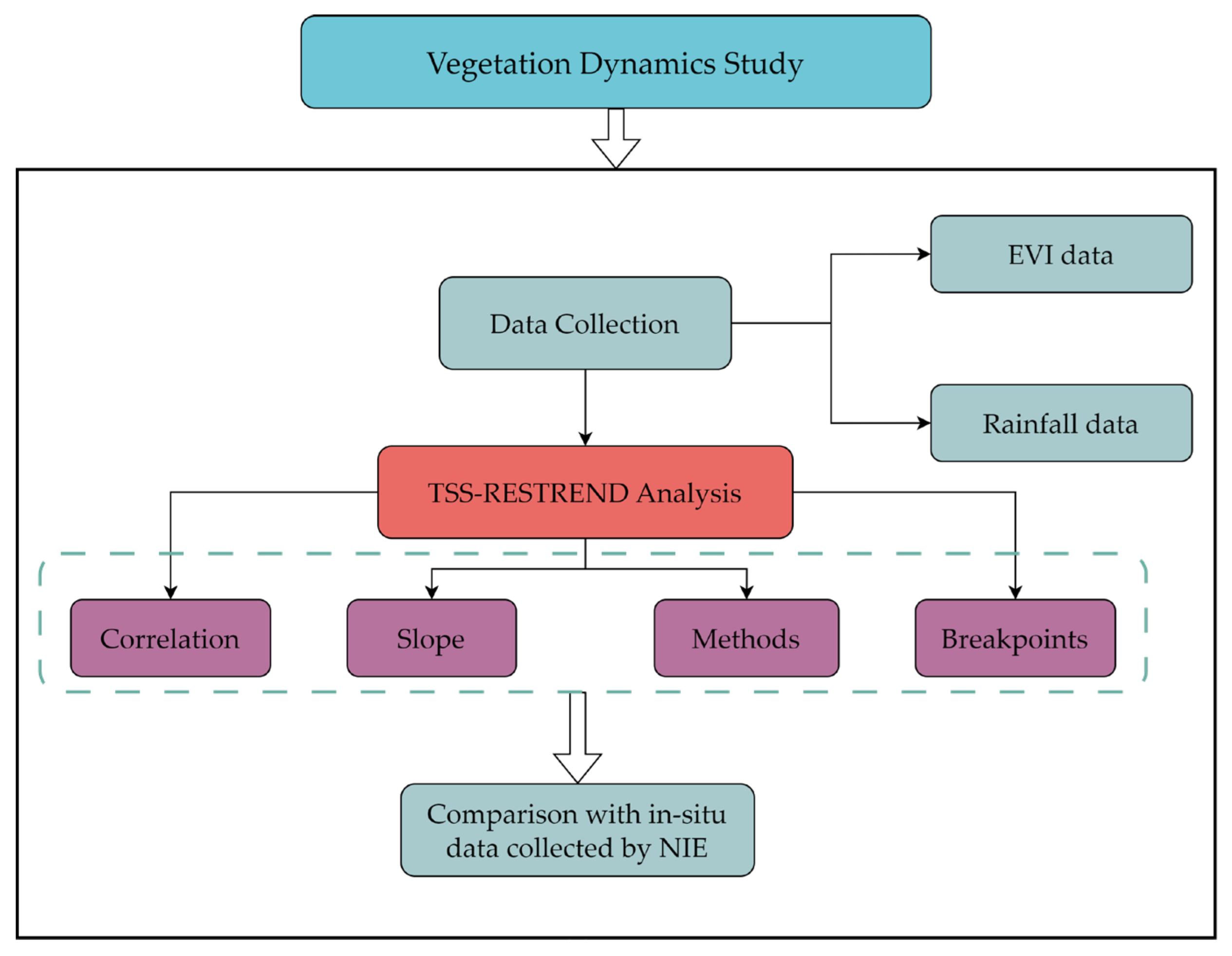
2. Materials and Methods

2.1. Study Area and Data

The research area covered the entire country of South Korea (Figure 2 and Figure 3), which has undergone major changes impacting vegetation cover and vegetation dynamics [29]. The region has experienced significant impacts due to climate change and to sustain urbanization and industrialization [30]. According to Köppen–Geiger climate classification (Figure 2), most of the country (57.2%) falls under the ‘Dwa’ category, indicating a dry winter and hot summer climate. Along the coast, the climate is temperate with hot summers and no dry season (Cfa).
One of the most notable changes in the country’s climate is the increase in air temperature fluctuations throughout the seasons. There has been a rapid decrease in the number of days with record low temperatures and a corresponding increase in maximum precipitation during the summer [21,31,32]. The Korean Ministry of Environment has published several climate change assessment reports, including the most recent one in 2020. These reports cover the ecological impacts of climate change and adaptation policies and plans in various sectors such as water resources, ecosystem services, forestry, agriculture, energy, health, human settlement, and welfare.
To study the dominant land covers in the country, the MODIS landcover product (MCD12Q1) from 2001 to 2020 with a spatial resolution of 500 m was used. The analysis of land cover data during the twenty-year period showed the four most prevalent land covers were deciduous broadleaf forests, mixed forests, wood savannas, and croplands as per IGBP (International Geosphere–Biosphere Programme) classification. On average, these land cover types accounted for more than 80% of the country’s land area over the last 20 years (Figure 4). There has been a sharp rise in deciduous broadleaf forests from 29.4% in 2001 to 34.25% in 2008, whereas the other land cover types have generally been unchanged, with a slight decrease of approximately 10% in croplands (20.8% in 2001 to 18.3% in 2020).
The in situ vegetation data utilized in this study was collected by the National Ecosystem Survey (NES) from 2006 to 2018. The NES covers the entire mountainous areas in South Korea during the predefined survey periods, excluding nationally protected or access-limited areas such as national parks and the Korean Demilitarized Zone. This data was collected in two distinct survey periods: 2006–2013 and 2014–2018. In situ vegetation data, which represents the top canopy layer and was confirmed by the field observations, was retrieved from EcoBank (https://www.nie-ecobank.kr; Access: 16 August 2023). The NES collected vegetation data in the mountains located in the assigned grids in a 1:25,000 scale map of South Korea each year using 20 m × 20 m quadrats. Field researchers of the NES initially recorded the top canopy layer into two categories based on dominant species: (1) single-species dominant vegetation, where a species covers more than 70% of the top canopy layer (e.g., Quercus variabilis forest); (2) two-species dominant vegetation, where a single species cannot cover more than 70% of the top canopy layer (e.g., Quercus variabilis–Quercus mongolica forest). The top canopy layer categories, which cover more than 90% of the entire survey area, were used for further analysis. We applied the land use class definitions of the IGBP to utilize the NES vegetation data as high-resolution ground truth data.
We analyzed rainfall data to examine whether there are shifts in rainfall related to the changes in the cover of deciduous broadleaf forests. Daily rainfall data, with a spatial resolution of 0.01°, from 1 January 2001 to 31 December 2019, was collected from the Korean Meteorological Department (Figure 5). Figure 5 shows the annual variation in monthly rainfall calculated for the entire country, revealing significant variability, with a substantial range in rainfall values across different months. Some months, such as May, July, August, October, and November exhibit a wider spread between the quartiles, indicating potential seasonal variations in the rainfall pattern during these months.
The highest monthly rainfall was recorded in July 2011, while the lowest was recorded in January 2011 (Figure 6). The difference between these two months exceeded 550 mm, suggesting the presence of extreme events. Such events could significantly impact the forests, affecting vegetation health. In the context of air temperature, the highest temperature was recorded in August 2011 (24.5 °C) and the lowest was recorded in January 2015 (−8.7 °C). The temperature data appears to follow a pattern similar to that of the rainfall; however, there are some irregularities, such as the high temperatures in July 2006. Such deviations might have implications for the phenological cycles and health of the deciduous broadleaf forests, potentially leading to shifts in their growth patterns and ecosystem dynamics. These significant temperature fluctuations could pose challenges to the resilience of deciduous broadleaf forests. Understanding how these ecosystems adapt to such variations and identifying vulnerable periods is crucial in developing effective conservation and management strategies, thus prompting the need to study the vegetation–precipitation relationship (VPR). All the datasets used in this study are presented in Table 1.
The study used EVI data collected from the MODIS product, MOD13Q1, which is produced in sixteen-day intervals with a spatial resolution of 250 m. Rainfall data were collected from the Korean Meteorological Department, provided as a daily product with a spatial resolution of approximately 100 m. To match the vegetation data, daily rainfall values were converted to those for 16 days by summing up the values. The EVI and aggregated rainfall data were used for a TSS-RESTREND approach, which is elaborated upon in the subsequent section.

2.2. TSS-RESTREND

The TSS-RESTREND approach involves establishing a statistical relationship between climate and vegetation, building upon the foundational residual trend (RESTREND) method used to assess seasonal phenological patterns for detecting structural alterations. To provide a more comprehensive understanding, the method integrates a modified version of the Breaks for Additive Seasonal and Trend (BFAST) technique, enabling the identification of structural modifications within ecosystems that may otherwise go unnoticed [27]. Given the prevalence of dense vegetation in the study area, a non-linear relationship exists between vegetation and climate [33]. However, a linear relationship can be expected between vegetation and the natural logarithm of rainfall, thereby enhancing the efficacy of RESTREND in forested environments [27,33]. Overall, the method has five steps:
(1)
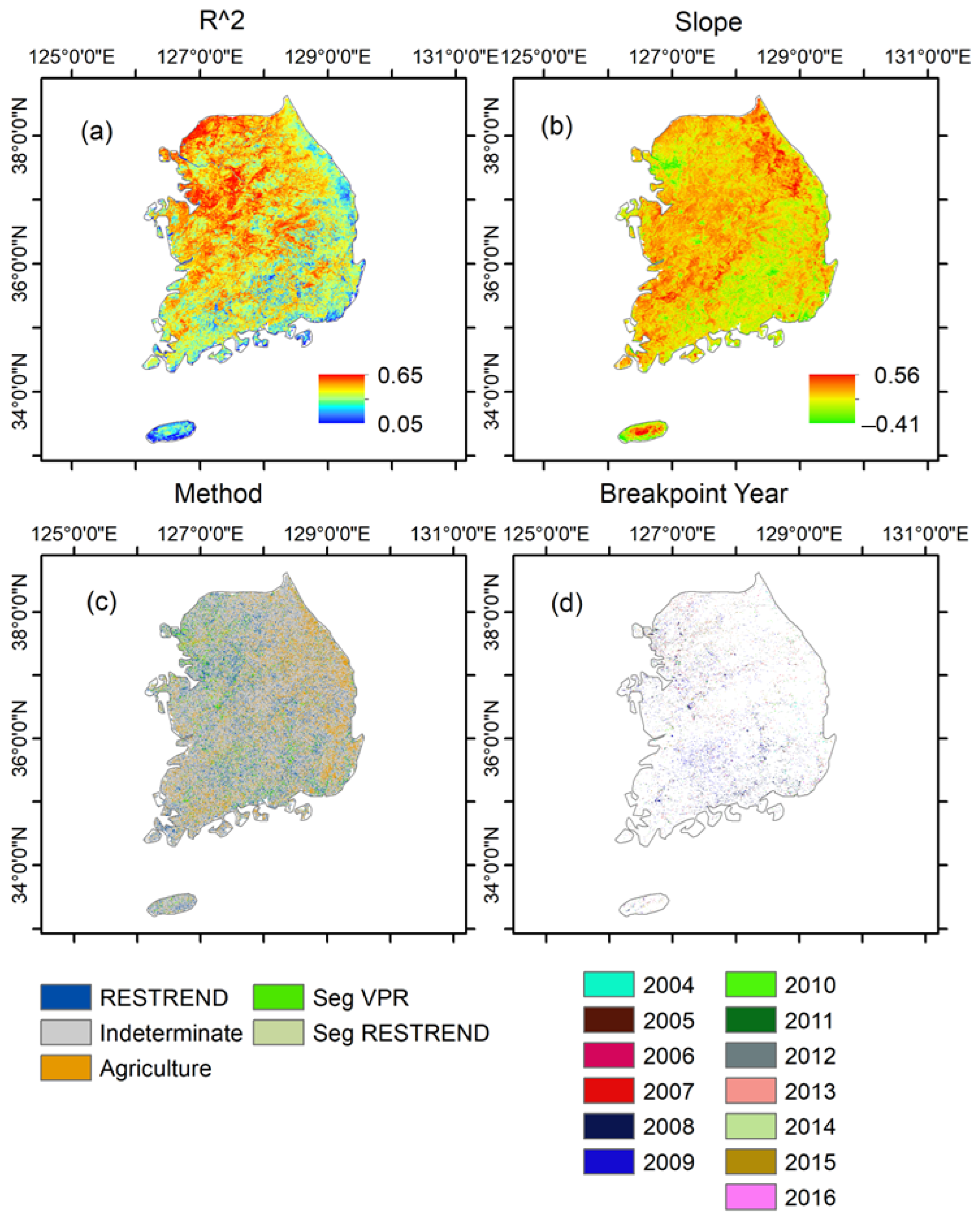
VPR computation involves ordinary least squares regression, which models the association between the annual EVI and the logarithm of the optimal accumulated precipitation. Optimal accumulated precipitation is determined on a per-pixel basis, identifying the accumulation period (1–24 time periods) and off-set period (1–3 time periods) that yield the highest correlation coefficients with EVImax in a calendar year. The disparity between the observed EVI and the EVI predicted by the identified VPR at each time step is recognized as the VPR residual.
(2)
BFAST is employed on the VPR residuals, now regulated for rainfall. The statistically significant breakpoints detected by the BFAST method throughout the time series necessitate further testing of their impact on primary productivity (EVImax). For pixels with a significant VPR (α = 0.05), a Chow Test [34] is utilized on the VPR residuals for this purpose.
(3)
The segmented RESTREND procedure involves conducting a multivariate regression among the VPR residuals, time, and a dummy variable, which is 0 before the breakpoint and 1 after it. The significance of the model is evaluated using the Chow test F statistic, while the direction of the change is determined by the discrepancy in the anticipated values between the beginning and end of the time series. Although its impacts are substantial, they are not significant enough to alter the ecosystem structure and disrupt VPR consistency. The significance of a VPR breakpoint is also assessed for pixels that did not pass the VPR significance test (p < 0.05).
(4)
A significant VPR breakpoint in a pixel suggests that there may have been notable structural changes to the ecosystem during the time series [35]. Hence, it cannot be assumed that the accumulation period and offset period utilized to calculate the optimal accumulated precipitation remain equivalent on either side of the breakpoint. To address this, the EVImax time series is partitioned, and VPR is recalculated separately on each side of the breakpoint.
The model produces four different outputs: (a) the correlation coefficient between the EVImax and cumulative rainfall, (b) the linear regression slope, (c) the method, and (d) the breakpoints, which highlight significant fluctuations in the relationship between the variables. The term “method” refers to the specific algorithmic procedures involved in determining the significant correlations and breakpoints within the dataset. The calculation techniques rely on the importance of VPR and breakpoints and are categorized into five distinctive groups, as follows: (1) indeterminate cases lacking significant VPR and significant breakpoints; (2) agricultural regions characterized by negative VPR values often associated with changes in agricultural practices; (3) RESTREND values indicating significant VPR without notable breakpoints in either the residual change trend or VPR; (4) segmented VPR values encompassing pixels exhibiting changes in both VPR and the residual trend; and (5) segmented RESTREND values emphasizing significant breakpoints solely within the residual trend [36].

3. Results

3.1. TSS-RESTREND Results

Figure 7 shows the different outputs of the overall trend pixel-wise using EVI and log rainfall from 2001–2020. Figure 7a shows the coefficient correlation and Figure 7b shows the slope of the VPR. The correlation is high in the northern part of the country, and gradually decreases toward the western boundaries. Similar patterns can be observed for the slope, indicating a strong relationship between vegetation and rainfall. In Figure 7c, the dominant method is ‘Indeterminate’, indicating that the relationship between vegetation and rainfall is not solely explained by each other, given the complex influence of other environmental factors.
A considerable portion, accounting for 14% of the area, represents agricultural regions characterized by negative VPR values (Table 2). These negative VPR values are often linked to changes such as the introduction of new crop varieties, innovative farming practices, and irrigation systems. The prevalence of this category emphasizes the significant impact of agricultural activities on the local environment, contributing to noteworthy modifications in the vegetation–climate relationship. Additionally, the areas classified under the Seg VPR and Seg RESTREND categories are relatively smaller, constituting 4.62% and 0.74% of the total area, respectively. These categories highlight significant changes in the VPR and breakpoints, with segmented VPR encompassing pixels exhibiting noteworthy alterations in both the VPR and the residual trend and segmented RESTREND emphasizing significant breakpoints solely within the residual trend. The variations in TSS-RESTREND methods underscore localized environmental variations and structural modifications within specific regions, signifying critical areas where the vegetation–climate relationship has undergone substantial changes.
Out of the 5,692,023 pixels comprising the study area, over 5.36% of the region had breakpoints at different points during the studied time period. The year-wise percentage of breakpoints (Table 3) demonstrates notable fluctuations, indicating periods of significant environmental changes within the study region.
However, the degree of environmental changes can differ based on the breakpoint percentage. For example, the years 2009 and 2012 stand out, constituting 23.38% and 22.79% of the total breakpoints, respectively. These findings suggest that substantial ecosystem shifts and alterations occurred during these years, highlighting the heightened vulnerability and sensitivity of the region to external factors during these specific periods. Likewise, the year 2008 displays a significant proportion of breakpoints, amounting to 16.59%. This observation accentuates the pivotal role of the environmental conditions prevalent during this year, possibly indicating critical shifts or disturbances within the ecosystem. Similarly, the years 2007 and 2015 also exhibit noteworthy percentages of breakpoints, accounting for 5.92% and 6.38% of the total breakpoints, respectively. These findings emphasize the significance of these years in terms of environmental changes and potential disturbances impacting the vegetation and climate relationship. The remaining years demonstrate relatively lower percentages of breakpoints, ranging from 2.46% to 3.53%. Although these years indicate comparatively fewer significant structural alterations, they provide insights into periods of relative stability and consistency within the ecosystem.
In 2012, the Korean forest area damaged by wildfires was at its lowest. Additionally, despite a yearly decrease of 1.3% in the total agricultural area, 2009 and 2012 stand out as the two years with the most significant proportional increases in the total dry crop field area compared to their respective preceding years. This is due to the major disturbances in rainfall and air temperature during this period, resulting in frequent occurrences of hydrometeorological hazards such as floods and droughts. For example, the country experienced extreme drought after 5–6 years, with the worst drought occurring in 2014–2015 [37]. This phenomenon can also be explained using box-and-whisker plot, which shows variations in monthly rainfall for the deciduous broadleaf forest region. Large variations in rainfall, especially in the months of January and October, indicate signs of extreme changes in climatic variables.

3.2. Comparison with In Situ Data

The premier ecological agency of South Korea, the National Institute of Ecology, collects in situ vegetation data which comprehensively surveys the entire country in a period of pre-defined years and provides various vegetation and plant data. The previous surveys were conducted from 2006–2013 and from 2014–2018. Based on the limited available data, deciduous broadleaf forests for these two different time periods were examined (Figure 8). As Figure 8 shows, there was an increase in forests from 2014–2018 compared to 2006–2013, as seen from the NIE data. Hence, to analyze the changes, high resolution vegetation images are needed to provide a better understanding of the vegetation dynamics in the region.
When comparing the in situ vegetation data of South Korea with the MCD12Q1 land cover product from the MODIS, a noticeable difference in the spatial coverage becomes apparent. Several factors contribute to this contrast; for example, the in situ data collection process involves manual or localized measurements, resulting in limited spatial representation, especially across heterogeneous and diverse landscapes such as South Korea. On the other hand, the MODIS product, derived from satellite imagery, offers extensive coverage and captures data from a broader perspective, encompassing various land cover types and regional variations. Additionally, the differences between the in situ data and the MODIS product could arise due to variations in the sampling methodologies, data processing techniques, and the categorization techniques.

4. Discussion

TSS-RESTREND, an innovative method for assessing vegetation dynamics in relation to climate variables, has emerged as a crucial tool in the realm of environmental monitoring and ecosystem analysis. By integrating EVI and rainfall data, the TSS-RESTREND method enables the identification and characterization of structural changes within the vegetation cover, offering valuable insights into the complex interactions between climate patterns and ecological systems. In the context of South Korea, a region characterized by diverse topography, distinct seasonal variations, and significant land cover heterogeneity, the application of the TSS-RESTREND method assumes significant importance for regeneration programs. This technique not only facilitates the comprehensive understanding of the intricate relationships between vegetation dynamics and climatic influences but also holds the potential to unravel the impacts of environmental changes on the country’s diverse ecosystems and natural landscapes. Furthermore, the utilization of TSS-RESTREND in South Korea aids in elucidating the implications of climate variability and land cover transformations for various ecological processes, thus contributing to informed decision-making, sustainable resource management, and the preservation of the country’s rich biodiversity.
The application of the TSS-RESTREND method revealed distinctive insights into vegetation dynamics and their relationship with climatic variables across the region. The dominance of the ‘Indeterminate’ category (69.21%) suggests the prevalence of areas where the vegetation–climate relationship lacks significant breakpoints, possibly indicating a stable ecological system or the influence of multiple confounding factors. Additionally, the notable presence of ‘Agricultural Regions’ (14.04%) underscores the sensitivity of certain areas to anthropogenic activities, including evolving agricultural practices and land-use changes. The relatively low prevalence of ‘Seg RESTREND’ (0.74%) signifies the limited occurrences of significant breakpoints solely in the residual, hinting at the relatively stable nature of the ecosystem across large portions of the region. Notably, our analysis identified a compelling spatial trend: the correlation strength is most pronounced in the northern territories and gradually diminishes as we traverse towards the western boundaries. A similar pattern is discerned for the slope, signifying a robust association between vegetation dynamics and rainfall. It is important to note that the eastern areas of South Korea are predominantly covered by vegetation in mountainous terrains, whereas the western regions are characterized by lowlands, with significant anthropogenic activities such as agriculture and urbanization. Therefore, our results underscore the regional heterogeneity—in terms of topography, climate zones, and other land use factors—and its profound influence on the vegetation–climate interplay in South Korea.
The discrepancies observed between the in situ vegetation data and the MODIS land cover product underscore the significant disparities in spatial coverage across South Korea. The stark differences between the two datasets accentuate the crucial role played by in situ data in capturing nuanced ecological variations and local intricacies, especially within heterogeneous landscapes such as South Korea. Given the pronounced variations in land cover types and their spatial distribution, the utilization of in situ data becomes indispensable in providing detailed insights into the localized ecological changes, particularly within regions where the MODIS data may fail to capture subtle shifts or unique ecosystem characteristics.
Although the country has seen a population growth of almost 10% during this period, its impact on land cover has been minimal. Cho et al. [29] studied ecosystem management in the country from 1918–2005. The study found an increase of over 70% (~7000 ha) in the vegetation cover during this period alongside a simultaneous increase in infrastructure development. The authors attributed this phenomenon to the country’s land management policy. Shah et al. [38] conducted spatio-temporal analysis of precipitation variation across the Han River basin, South Korea and found an increase in rainfall from south to north, suggesting the region suffers from extreme floods during the summer and severe droughts in winter. In the case of air temperature, the difference is less than 10% across all land covers. A previous study by Jung et al. [31] which studied the air temperature trends of 12 stations in South Korea from 1954–1999 found an upward trend of 0.23 °C per decade. The minimal impact on temperature can be attributed to expanding vegetated areas, especially in areas which have seen rapid rise in urbanization. Hwang et al. [39] studied the NDVI trends in Seoul, South Korea and found an increasing trend, which resulted from planting trees in impervious regions, such as streets, and found an increase in vegetation growth in forests. This trait can be extrapolated for the entire country, as can be seen in the trends of vegetation (Figure 4).
The comprehensive TSS-RESTREND analysis has shown the critical role played by both in situ data and remote sensing products in understanding the dynamic landscape changes within South Korea. The comparative analysis of these datasets has highlighted the necessity of using in situ data to capture local ecological intricacies and its significant contribution towards validating and refining remote sensing-based observations. The use of in situ data along with the TSS-RESTREND framework serves as a valuable tool for monitoring the efficacy of ecological restoration initiatives, particularly within regions characterized by diverse vegetation and heterogeneous landscapes. These findings emphasize the necessity of a multi-faceted approach that combines both ground-based observations and satellite-derived data to comprehensively assess and manage the intricate ecological dynamics of South Korea’s diverse landscapes. This analysis is particularly pertinent in the context of South Korea’s extensive forest regeneration program, which has significantly influenced the landscape and vegetation patterns in various regions, further emphasizing the critical role of in situ data in monitoring and assessing the outcomes of large-scale ecological restoration initiatives.

5. Conclusions

South Korea has experienced a significant surge in urbanization over the last 50 years which has greatly impacted the region’s land cover and land use and, subsequently, the regional climate and ecohydrological balance. In this study, TSS-RESTREND analysis integrated with in situ vegetation data and MODIS remote sensing products provided valuable insights into the spatiotemporal dynamics of South Korea’s vegetation. The comprehensive analysis of the vegetation’s response to rainfall variability has not only facilitated the identification of structural changes in the ecosystem but has also underscored the critical role played by both ground-based observations and satellite-derived data in monitoring and managing ecological landscapes. The findings from this study emphasize the significance of integrating multi-sourced data to enhance our understanding of complex ecological processes, thereby facilitating more effective and targeted conservation and restoration efforts. The comparison between in situ data and MODIS observations has highlighted the necessity of continuous ground-level data collection to validate and complement remote sensing data, especially in regions characterized by diverse landscapes and varying ecological patterns. Moreover, the examination of the spatial coverage disparities has reinforced the need for sustained efforts in data collection to bridge the gaps between ground-based and satellite observations, thereby facilitating more accurate and holistic assessments of landscape dynamics. The country has plans for targeted forest regeneration activities, and this comprehensive analysis provides a quantifiable metric to examine the climatic impacts and changes in land use. The insights learned from this research can inform and guide future conservation strategies and policy frameworks aimed at promoting sustainable land management and ecosystem preservation in South Korea.

Author Contributions

Conceptualization, B.P., S.Y. and S.L.; methodology, B.P., S.Y. and S.L.; software, B.P.; validation, B.P., S.Y. and S.L.; formal analysis, B.P.; investigation, B.P. and S.Y.; resources, B.P. and S.Y.; data curation, B.P. and S.Y.; writing—original draft preparation, B.P., S.Y. and S.L.; writing—review and editing, B.P., S.Y. and S.L.; visualization, S.L.; supervision, B.P., S.Y. and S.L.; project administration, B.P., S.Y. and S.L.; funding acquisition, B.P., S.Y. and S.L. All authors have read and agreed to the published version of the manuscript.

Funding

This research was funded by the National Institute of Ecology (NIE), grant number NIE-B-2024-01.

Data Availability Statement

No new data were created or analyzed in this study. Data are contained within the article.

Conflicts of Interest

The authors declare no conflict of interest.

References

  1. Foley, J.A.; Levis, S.; Costa, M.H.; Cramer, W.; Pollard, D. Incorporating dynamic vegetation cover within global climate models. Ecol. Appl. 2000, 10, 1620–1632. [Google Scholar] [CrossRef]
  2. Chu, H.S.; Venevsky, S.; Wu, C.; Wang, M. NDVI-based vegetation dynamics and its response to climate changes at Amur-Heilongjiang River Basin from 1982 to 2015. Sci. Total Environ. 2019, 650, 2051–2062. [Google Scholar] [CrossRef] [PubMed]
  3. Pan, N.; Feng, X.; Fu, B.J.; Wang, S.; Ji, F.; Pan, S. Increasing global vegetation browning hidden in overall vegetation greening: Insights from time-varying trends. Remote Sens. Environ. 2018, 214, 59–72. [Google Scholar] [CrossRef]
  4. Yang, D.; Shao, W.; Yeh, P.J.-F.; Yang, H.; Kanae, S.; Oki, T. Impact of vegetation coverage on regional water balance in the nonhumid regions of China. Water Resour. Res. 2009, 45. [Google Scholar] [CrossRef]
  5. Franklin, J.; Serra-Diaz, J.M.; Syphard, A.D.; Regan, H.M. Global change and terrestrial plant community dynamics. Proc. Natl. Acad. Sci. USA 2016, 113, 3725–3734. [Google Scholar] [CrossRef]
  6. Sun, G.; Hallema, D.; Asbjornsen, H. Ecohydrological processes and ecosystem services in the Anthropocene: A review. Ecol. Process. 2017, 6, 35. [Google Scholar] [CrossRef]
  7. Dikshit, A.; Pradhan, B.; Huete, A.; Park, H.J. Spatial based drought assessment: Where are we heading? A review on the current status and future. Sci. Total Environ. 2022, 844, 157239. [Google Scholar] [CrossRef]
  8. Yang, S.; Liu, J.; Wang, C.; Zhang, T.; Dong, X.; Liu, Y. Vegetation dynamics influenced by climate change and human activities in the Hanjiang River Basin, central China. Ecol. Indic. 2022, 145, 109586. [Google Scholar] [CrossRef]
  9. Zhao, C.; Yan, Y.; Ma, W.; Shang, X.; Chen, J.; Rong, Y.; Xie, T.; Quan, Y. RESTREND-based assessment of factors affecting vegetation dynamics on the Mongolian Plateau. Ecol. Model. 2021, 440, 109415. [Google Scholar] [CrossRef]
  10. Frappart, F.; Wigneron, J.-P.; Li, X.; Liu, X.; Al-Yaari, A.; Fan, L.; Wang, M.; Moisy, C.; Le Masson, E.; Lafkih, Z.A.; et al. Global Monitoring of the Vegetation Dynamics from the Vegetation Optical Depth (VOD): A Review. Remote Sens. 2020, 12, 2915. [Google Scholar] [CrossRef]
  11. Wen, L.; Mason, T.J.; Ryan, S.; Ling, J.E.; Saintilan, N.; Rodriguez, J. Monitoring long-term vegetation condition dynamics in persistent semi-arid wetland communities using time series of Landsat data. Sci. Total Environ. 2023, 905, 167212. [Google Scholar] [CrossRef] [PubMed]
  12. Li, S.; Xu, L.; Chen, J.; Jiang, Y.; Sun, S.; Yu, S.; Tan, Z.; Li, X. Monitoring vegetation dynamics (2010–2020) in Shengnongjia Forestry District with cloud-removed MODIS NDVI series by a spatio-temporal reconstruction method. Egypt. J. Remote Sens. Space Sci. 2023, 26, 527–543. [Google Scholar] [CrossRef]
  13. Abbas, S.; Qamer, F.M.; Ali, H.; Usman, M.; Ahmad, A.; Salman, A.; Akhter, A.M. Monitoring of large-scale forest restoration: Evidence of vegetation recovery and reversing chronic ecosystem degradation in the mountain region of Pakistan. Ecol. Inform. 2023, 77, 102277. [Google Scholar] [CrossRef]
  14. Caparros-Santiago, J.A.; Quesada-Ruiz, L.C.; Rodriguez-Galiano, V. Can land surface phenology from Sentinel-2 time-series be used as an indicator of Macaronesian ecosystem dynamics? Ecol. Inform. 2023, 77, 102239. [Google Scholar] [CrossRef]
  15. Huete, A.; Didan, K.; Miura, T.; Rodriguez, E.P.; Gao, X.; Ferreira, L.G. Overview of the radiometric and biophysical performance of the MODIS vegetation indices. Remote Sens. Environ. 2002, 83, 195–213. [Google Scholar] [CrossRef]
  16. Wang, X.; Piao, S.; Ciais, P. Spring temperature change and its implication in the change of vegetation growth in North America from 1982 to 2006. Proc. Natl. Acad. Sci. USA 2011, 108, 1240–1245. [Google Scholar] [CrossRef]
  17. Bao, G.; Qin, Z.; Bao, Y.; Zhou, Y.; Li, W.; Sanjjav, A. NDVI-Based Long-Term Vegetation Dynamics and Its Response to Climatic Change in the Mongolian Plateau. Remote Sens. 2014, 6, 8337–8358. [Google Scholar] [CrossRef]
  18. Verger, A.; Filella, I.; Baret, F.; Peñuelas, J. Vegetation baseline phenology from kilometric global LAI satellite products. Remote Sens. Environ. 2016, 178, 1–14. [Google Scholar] [CrossRef]
  19. Yang, Q.; Zhang, H.; Peng, W.; Lan, Y.; Luo, S.; Shao, J.; Chen, D.; Wang, G. Assessing Climate Impact on forest Cover in Areas Undergoing Substantial Land Cover Change Using Landsat Imagery. Sci. Total Environ. 2019, 659, 732–774. [Google Scholar] [CrossRef]
  20. Lamchin, M.; Lee, W.-K.; Jeon, S.W.; Wang, A.W.; Lim, C.H.; Song, X.; Sung, M. Long-term trend of and correlation between vegetation greenness and climate variables in Asia based on satellite data. MethodsX 2018, 5, 803–807. [Google Scholar] [CrossRef]
  21. Kim, G.S.; Lim, C.-H.; Kim, S.J.; Lee, J.; Son, Y.; Lee, W.-K. Effect of national-scale afforestation on forest water supply and soil loss in South Korea, 1971–2010. Sustainability 2017, 9, 1017. [Google Scholar] [CrossRef]
  22. Ukasha, M.; Ramirez, J.A.; Niemann, J.D. Temporal variations of NDVI and LAI and interactions with hydroclimatic variables in a large and agro-ecologically diverse region. J. Geophys. Res. Biogeosci. 2022, 127, e2021JG006395. [Google Scholar] [CrossRef]
  23. Ghebrezgabher, M.G.; Yang, T.; Yang, X.; Sereke, T.E. Assessment of NDVI variations in responses to climate change in the Horn of Africa. Egypt. J. Remote Sens. Space Sci. 2020, 23, 249–261. [Google Scholar] [CrossRef]
  24. Verbesselt, J.; Hyndman, R.; Newnham, G.; Culvenor, D. Detecting trend and seasonal changes in satellite image time series. Remote. Sens. Environ. 2010, 114, 106–115. [Google Scholar] [CrossRef]
  25. Jönsson, P.; Eklundh, L. TIMESAT—A program for analyzing time-series of satellite sensor data. Comput. Geosci. 2004, 30, 833–845. [Google Scholar] [CrossRef]
  26. Guo, M.; Li, J.; He, H.; Jiawei, X.; Yinghua, J. Detecting Global Vegetation Changes Using Mann-Kendal (MK) Trend Test for 1982–2015 Time Period. Chin. Geogr. Sci. 2018, 28, 907–919. [Google Scholar] [CrossRef]
  27. Wessels, K.J.; van den Bergh, F.; Scholes, R.J. Limits to detectability of land degradation by trend analysis of vegetation index data. Remote Sens. Environ. 2012, 125, 10–22. [Google Scholar] [CrossRef]
  28. Liu, Z.; Menzel, L. Identifying long-term variations in vegetation and climatic variables and their scale-dependent relationships: A case study in Southwest Germany. Glob. Chang. Biol. 2016, 147, 54–66. [Google Scholar] [CrossRef]
  29. Cho, Y.-C.; Kim, N.-S.; Koo, B.-Y. Changed land management policy and the emergence of a novel forest ecosystem in South Korea: Landscape dynamics in Pohang over 90 years. Ecol. Res. 2018, 33, 351–361. [Google Scholar] [CrossRef]
  30. Korea Meteorological Administration (KMA). Summary of Korea Global Atmosphere Watch 2011 Report. KMA, Seoul, Republic of Korea, 2012; Volume 201, p. 10. [Google Scholar]
  31. Jung, H.-S.; Choi, Y.; Lim, G.-H. Recent Trends in Temperature and Precipitation over South Korea. Int. J. Clim. 2022, 22, 1327–1337. [Google Scholar] [CrossRef]
  32. Choi, S.W.; Kong, W.S.; Hwang, G.-Y.; Ah Koo, K. Trends in the effects of climate change on terrestrial ecosystems in the Republic of Korea. J Ecol. Environ. 2021, 45, 13. [Google Scholar] [CrossRef]
  33. Wessels, K.J.; Prince, S.D.; Malherbe, J.; Small, J.; Frost, P.E.; VanZyl, D. Can human-induced land degradation be distinguished from the effects of rainfall variability? A case study in South Africa. J. Arid Environ. 2007, 68, 271–297. [Google Scholar] [CrossRef]
  34. Chow, G.C. Tests of equality between sets of coefficients in two linear regressions. Econometrica 1960, 28, 591–605. [Google Scholar] [CrossRef]
  35. Fensholt, R.; Horion, S.; Tagesson, T.; Ehammer, A.; Grogan, K.; Tian, F.; Huber, S.; Verbesselt, J.; Prince, S.D.; Tucker, C.J.; et al. Assessing drivers of vegetation changes in drylands from time series of earth observation data. In Remote Sensing Time Series, Remote Sensing and Digital Image Processing; Kuenzer, C., Dech, S., Wagner, W., Eds.; Springer International Publishing: Berlin/Heidelberg, Germany, 2015; pp. 183–202. [Google Scholar]
  36. Li, Z.; Wang, S.; Song, S.; Wang, Y.; Musakwa, W. Detecting land degradation in Southern Africa using Time Series Segment and Residual Trend (TSS-RESTREND). J. Arid Environ. 2021, 184, 104314. [Google Scholar] [CrossRef]
  37. Hong, I.; Lee, J.-H.; Cho, H.-S. National drought management framework for drought preparedness in Korea (lessons from the 2014–2015 drought). Water Policy 2016, 18, 89–106. [Google Scholar] [CrossRef]
  38. Shah, A.A.; Jehanzaib, M.; Kim, J.I.; Kwak, D.-Y.; Kim, T.-W. Spatial and Temporal Variation of Annual and Categorized Precipitation in the Han River Basin, South Korea. KSCE J. Civ. Eng. 2022, 26, 1990–2001. [Google Scholar] [CrossRef]
  39. Hwang, Y.; Ryu, Y.; Qu, S. Expanding vegetated areas by human activities and strengthening vegetation growth concurrently explain the greening of Seoul. Landsc. Urban Plan. 2022, 227, 104518. [Google Scholar] [CrossRef]
Figure 1. Flowchart of the present study.
Remotesensing 16 00300 g001
Figure 2. Köppen–Geiger climate classification map of South Korea.
Remotesensing 16 00300 g002
Figure 3. (a) Average rainfall and (b) average air temperature for South Korea from January 2001–December 2019 (Source: South Korean Meteorological Department).
Remotesensing 16 00300 g003
Figure 4. The percentage of area covered by the three most important vegetation types (deciduous broadleaf forests, mixed forests, woody savannas, and croplands) in South Korea (Source: MODIS—MCD12Q1).
Remotesensing 16 00300 g004
Figure 5. Box and whisker plots showing the annual variation in monthly rainfall measures in deciduous broadleaf forests for 2001–2019. The bottom and top of the rectangular boxes are the 25th and 75th percentiles, respectively; the horizontal thick lines inside the boxes are the 50th percentiles (median values); the whiskers show 1.5 times the interquartile range; the points represent outliers.
Remotesensing 16 00300 g005
Figure 6. Monthly variation in the rainfall and temperature of deciduous broadleaf forests from January 2001 to December 2019.
Remotesensing 16 00300 g006
Figure 7. Vegetation–precipitation relationship results from the TSS-RESTREND method: (a) R2, (b) slope, (c) method, and (d) breakpoint year.
Remotesensing 16 00300 g007
Figure 8. Comparison of high spatial resolution images of deciduous broadleaf forests captured by the NIE and MODIS from 2006 to 2018.
Remotesensing 16 00300 g008
Table 1. Different satellite and in situ datasets used in this study.
Data TypeSourceSpatial ResolutionTime Period
Land coverMODIS (MCD12Q1)500 m2001–2019
EVIMODIS (MOD13Q1)250 m2001–2019
RainfallSouth Korean Meteorological Department0.01° × 0.01°
Air temperatureSouth Korean Meteorological Department0.01° × 0.01°
In situ vegetationNational Institute of Ecology20 m
Table 2. Percentage of pixels showing different TSS-RESTREND methods.
Method% of Area
RESTREND11.37
Indeterminate69.21
Agricultural Regions14.04
Seg VPR4.62
Seg RESTREND0.74
Table 3. Year-wise percentage of breakpoints.
Year% of PointsYear% of Points
20042.4920112.48
20053201222.79
20062.8320135.06
20075.9220142.46
200816.5920156.38
200923.3820163.04
20103.53
Disclaimer/Publisher’s Note: The statements, opinions and data contained in all publications are solely those of the individual author(s) and contributor(s) and not of MDPI and/or the editor(s). MDPI and/or the editor(s) disclaim responsibility for any injury to people or property resulting from any ideas, methods, instructions or products referred to in the content.

