Abstract
A unique End-of-Life (EOL) Deep Space View Test (DSVT) was performed on 27 November 2021 for the Advanced Microwave Sounding Unit-A (AMSU-A) and the Microwave Humidity Sounder (MHS) onboard the first EUMETSAT MetOp-A satellite in the deorbiting process. The purpose of this test is to recalibrate the antenna sidelobe, to derive antenna emission, and to quantify the in-orbit asymmetric scan biases of AMSU-A and MHS to, ultimately, improve Near Real-Time (NRT) products for MetOp-B and -C and the entire Fundamental Climate Data Records (FCDR). In this study, MetOp-A AMSU-A and MHS EOL DSVT data on 27 November 2021 have been analyzed. The deep space scene antenna temperatures were first applied for the antenna pattern correction; then, the antenna reflector channel emissivity values were derived from the corrected temperatures. For the MHS, the observed scan-angle-dependent brightness temperatures (BTs) for all channels were well behaved after the antenna pattern correction, except for channel 1. The derived antenna reflector emissivity values from this test are 0.0016, 0.0036, 0.0036, and 0.0019 for channels 1, 3, 4, and 5, respectively. For AMSU-A, the deep space view counts were not homogeneous during the test period, exhibiting large variations in the along-track and cross-track directions, mainly due to the instrument temperature’s rapid change during the test period. The large relative noise in the deep space view observations negatively impacted the data quality and limits the value of this test. The large relative noise may contribute to the different emissivity values derived from the same frequency for channels 9 to 14. We also found unexpected scan-angle-dependent BT after antenna pattern correction for quasi-vertical (QV) channels 1 and 2 when compared to the emission model. Further investigation using a simulation confirmed that channels 1 and 2 are QV channels, as designed.
1. Introduction
Since 1998 and continuing into the present day, the Advanced Microwave Sounding (AMSU, including Unit-A and Unit-B) and Microwave Humidity Sounder (MHS) have replaced the Microwave Sounding Unit (MSU) on various satellites, including the NOAA Polar Operational Environmental Satellite (POES) NOAA-15 through NOAA-19, NASA Aqua, and the EUMETSAT Polar System (EPS) Meteorological Operational Satellites (MetOp) series (MetOp-A/B/C). The AMSU-A offers enhanced capabilities, providing global temperature profile observations with 15 channels and higher vertical and horizontal resolutions, while the MHS, which replaced AMSU-B, provides humidity profile sounding capability with 5 channels [1]. The Advanced Technology Microwave Sounder (ATMS), currently onboard the Suomi National Polar-Orbiting Partnership (SNPP) and the NOAA Joint Polar Satellite System (JPSS) 1 and 2 (renamed to NOAA-20 and NOAA-21), represents the third generation of microwave sounders. The ATMS shares most of its channel frequencies with AMSU-A/MHS for temperature and humidity sounding and will continue NOAA’s microwave sounding capabilities with future JPSS satellites [2]. For nearly a quarter century, the observations from these microwave instruments have been pivotal for numerical weather prediction (NWP) and environmental monitoring [3]. Despite their primary focus on weather observations, these instruments are also essential for maintaining vital long-term global fundamental climate data records (FCDR) due to their extended operational periods, insensitivity to clouds, and global coverage [4].
These microwave instruments typically provide antenna temperature data records (TDR) in which the calibration equation assumes a weakly nonlinear sensor response and often neglects radiance contributions from antenna sidelobes [5,6,7,8,9], nonzero reflector antenna emissivity [10,11,12,13,14], and other uncertainties, such as a warm load temperature and emissivity [15]. Microwave sounding instruments often meet design specifications (which are primarily for weather applications) without correcting for these neglected contributions. However, the user community needs brightness temperature (BT) sensor data records (SDR) data to correct these neglected radiance contributions, which are instrument dependent and have impacts on instrument measurement biases and variability, as well as on numerical weather predication, environmental monitoring, and climate analysis. The conversion from TDR data to SDR data has been previously explored and applied to various space-borne radiometers to some degree. Notably, this conversion has been employed for the AMSU-A/MHS instruments on NOAA-15 to -19, as well as MetOp-A/B/C satellites [8,9,16]. While the legacy AMSU-A/MHS conversion algorithm primarily addressed sidelobe contributions based on prelaunch measurements, the ATMS conversion algorithm includes an additional correction for antenna emission contributions, utilizing data obtained during deep space pitch maneuvers for TDR to SDR corrections [13]. The SNPP was the first satellite to perform such a deep space pitch maneuver. The measurements demonstrated that the ATMS antenna plane reflector has small but nonnegligible emissions, especially for the cold calibration target (i.e., deep space) at a temperature of 2.728 K [12,13].
Launched on 19 October 2006, MetOp-A was placed into a sun-synchronous orbit and operated in tandem with MetOp-B and MetOp-C to form the EUMETSAT Polar System. After delivering vital meteorological data to a global user base for an impressive fifteen-year duration, surpassing its initial projected lifespan by three times, EUMETSAT made the decision to initiate its deorbiting process in November 2021. As part of its deorbiting procedure, MetOp-A underwent an End-of-Life (EOL) Deep Space View Test (DSVT) on 27 November 2021, based on insights from previous ATMS deep space pitch maneuvers conducted during the postlaunch test from the SNPP and NOAA-20 missions. It is noteworthy that no measurements of polarized emission from the AMSU-A/MHS antenna reflector were made on the ground prior to its launch. The primary objective of the DSVT was to quantify in-orbit asymmetric scan biases and perform on-orbit pitch-over maneuvers, essential for determining the actual polarized antenna emission. These efforts were carried out with the ultimate goal of improving Near Real-Time (NRT) products for both MetOp-B and MetOp-C, as well as enhancing the entire FCDR derived from microwave instruments.
This study focused on deriving the antenna reflector emissivity for MetOp-A AMSU-A and MHS instruments based on the Deep Space View Test data. Section 2 introduces the DSVT data, providing essential context for the subsequent analysis. In Section 3, we analyze the instrument noise and present the DSVT data after applying antenna pattern correction techniques and detail the process of deriving antenna reflector emissivity. Finally, Section 4 provides discussions and summaries of the study.
2. Deep Space View Test Data
The AMSU-A instrument operates in a cross-scan mode, with each scan lasting 8 s and comprising 30 Field of Views (FOVs) for Earth views (ES), 2 cold calibration target (DS) views, and 2 on-board warm target (ICT) views. Similarly, the MHS instrument also operates in a cross-scan mode and consists of 5 channels. Each scan lasts approximately 8/3 s and includes 90 FOVs for ES, along with four DS views and four ICT views.
The DSVT had a specific timeline outlined in Table 1. It started at UTC 10:30:09 and ended at UTC 10:36:35 on 27 November 2021, with a total duration of 386 s. During the analysis of the DSVT data, it was determined that extending the test duration slightly could mitigate the noise and variation presented in the data. The data used in this study were collected from 10:21 UTC to 10:40 UTC, just after the nadir limb and before commencement of the electromagnetic interference (EMI) test. This dataset consists of a total of 143 scan lines for AMSU-A and 428 scan lines for the MHS.

Table 1.
Deep space view test timeline. PSO (Position Sur l’Orbite, or position on the orbit) is the angular position of the spacecraft on its orbit. PSO is 0° at the ascending node and 180° at the descending node.
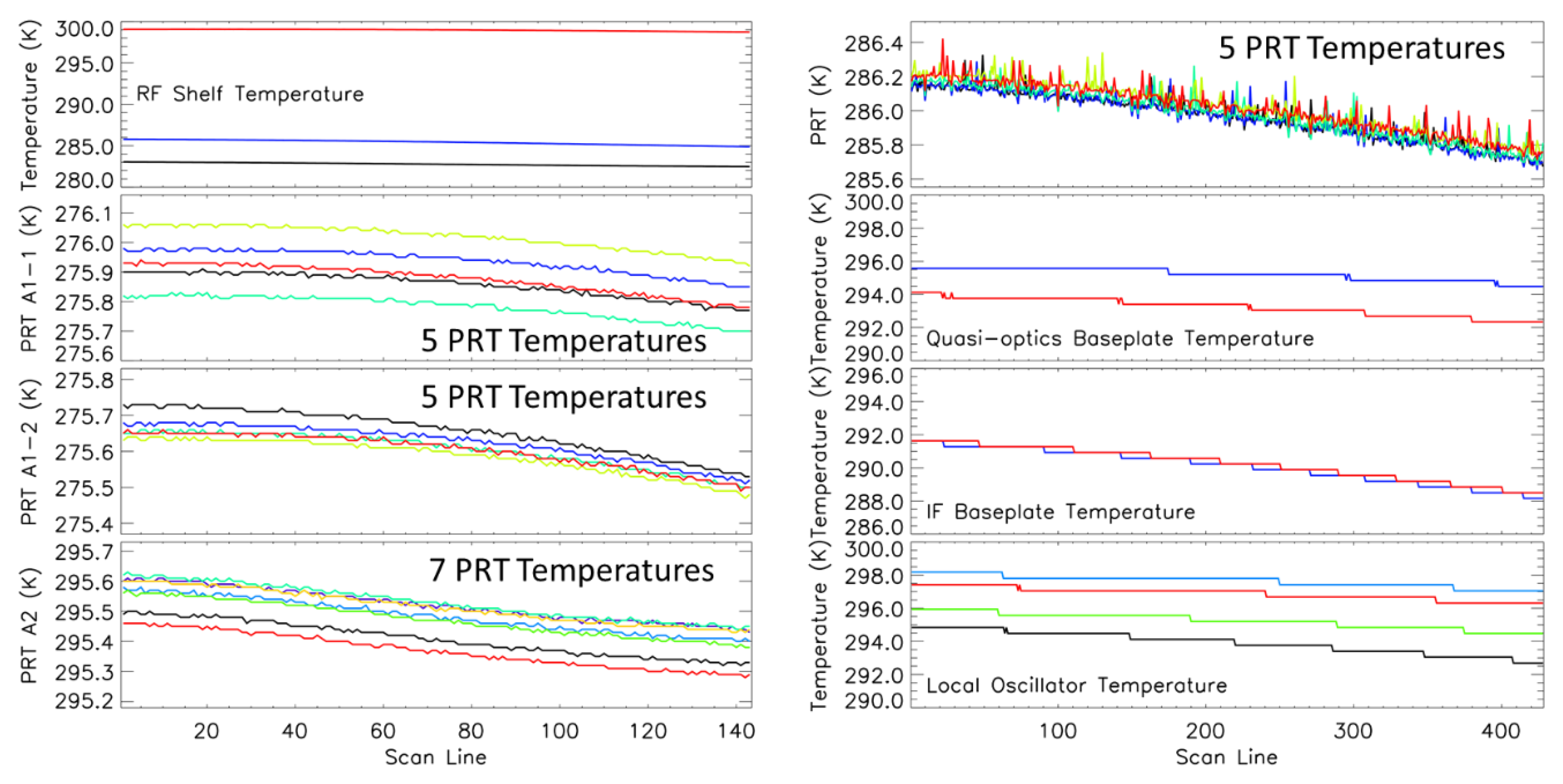
We initiated our analysis by examining the instrument temperatures for both AMSU-A and MHS during the specified period. Notably, AMSU-A comprises three separate units: AMSU-A2 is responsible for providing channels 1 and 2 at 23.8 and 31.4 GHz; AMSU-A1-2 includes channels 3–5 and 8; and AMSU-A1-1 furnishes channels 6, 7, and 9–15. In the left panel of Figure 1, we present the AMSU-A instrument temperatures, including the Radio Frequency (RF) Shelf Temperature for the various units (indicated by the black line for A1-1, blue line for A1-2, and red line for A-2), as well as the Platinum Resistance Thermometer (PRT) temperature for A1-1 (comprising a total of 5 PRTs), A1-2 (comprising a total of 5 PRTs), and A2 (comprising a total of 7 PRTs). It clearly shows that the RF shelf temperature and PRT temperatures gradually decreased over the course of the data collection period. In the right panel of Figure 1, we illustrate the MHS instrument temperatures, including the PRT temperatures (a total of 5 PRTs), temperatures of the quasi-optics baseplates (a total of 2), temperatures of the intermediate frequency (IF) baseplates (a total of 2), and the local oscillator temperature for each channel (with channels 3 and 4 sharing a single oscillator). A similar trend of decreasing temperatures is observed, notably in the IF baseplate temperature and PRT temperatures, during the data collection period. It is worth mentioning that small periodic spikes are evident in the PRT temperatures for the MHS during this period. We also analyzed other instrument-related temperatures, such as scan motor temperature, feed horn temperature, mixer/IF amplifier temperature, and detector/preamp assembly temperature. All of these temperatures decreased more rapidly and significantly during this period than under the normal Earth scan conditions.
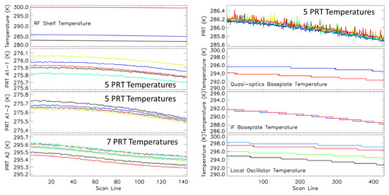
Figure 1.
AMSU-A (left) and MHS (right) instrument temperature during the DSVT period. Different colors in the RF shelf temperature are for the various AMSU-A units (black line for A1-1, blue line for A1-2, and red line for A-2); Different colors in PRT temperatures are for different individual PRT thermometer; There are two quasi-optics baseplate temperatures and two IF baseplate temperatures; and Different colors in local oscillator temperature are for different channels (black line for channel 1, blue line for channel 2, green line for channels 3 and 4, and red line for channel 5).
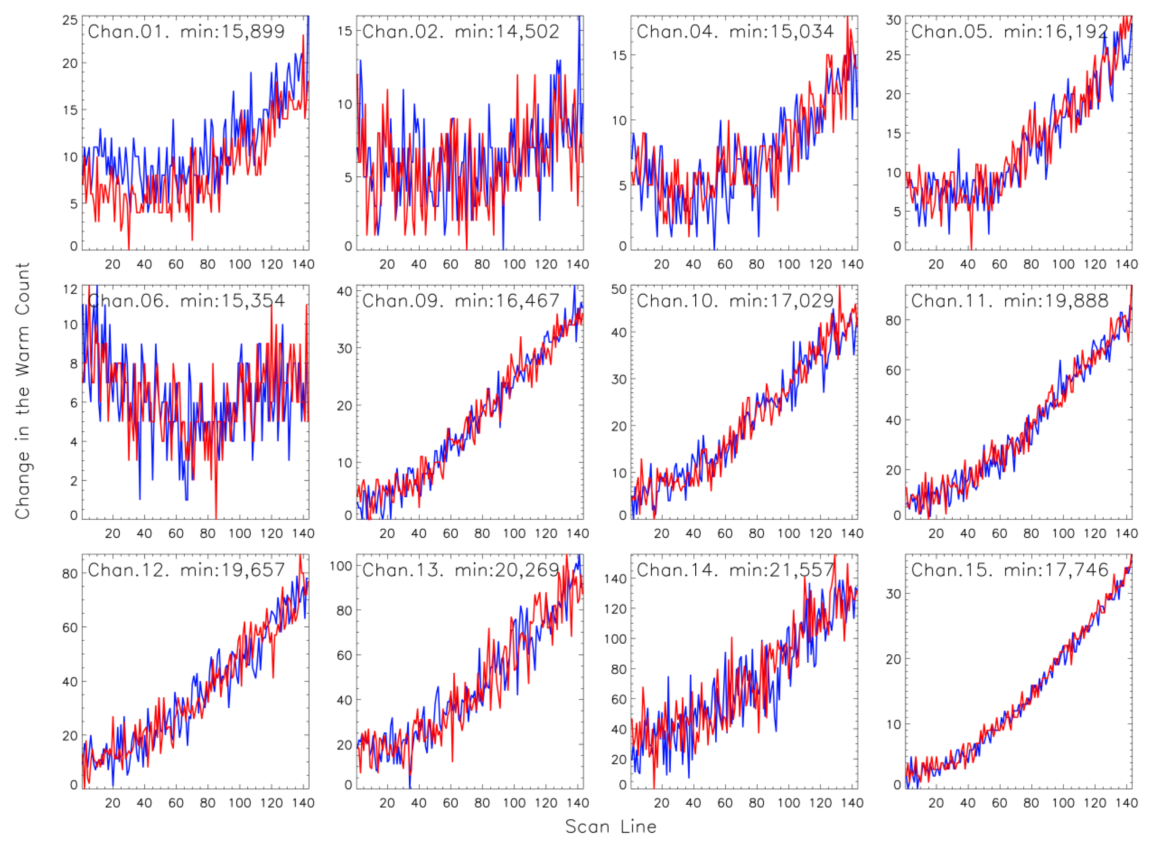
The examination of the AMSU-A’s performance during the test period involved an analysis of the cold counts and warm counts, which represent the cold calibration targets and warm calibration targets, respectively, in the radiometric calibration, as shown in Figure 2 and Figure 3, respectively. It is important to note that only the data from the good AMSU-A channels are presented here. Channels 7 and 8 experienced failure on 1 December 2009 and 18 April 2016, respectively. Additionally, channel 3 exhibited noise level consistently above the specification requirement (0.4 K) after 15 July 2013. Therefore, data from these three channels were excluded from our study. In Figure 2 and Figure 3, distinct colors, such as blue for target 1 and red for target 2, represent data from different calibration targets. For each channel, the y-axis represents the change in the count relative to its minimum count during the period. Both the cold counts and warm counts from the two calibration targets displayed significant fluctuations, with no distinct period of relative stability observed throughout the test period.
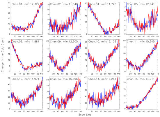
Figure 2.
Cold counts from AMSU-A channels during the DSVT period. Only good AMSU-A channels are shown here. Channels 7 and 8 failed, and the noise from channel 3 was well above the specification requirement. Different cold targets are shown separately using different colors (blue for target 1 and red for target 2). Note that for each channel the y-axis represents the change in the cold count related to its minimum count during the period.

Figure 3.
Same as Figure 2 but for warm counts from the warm calibration targets.
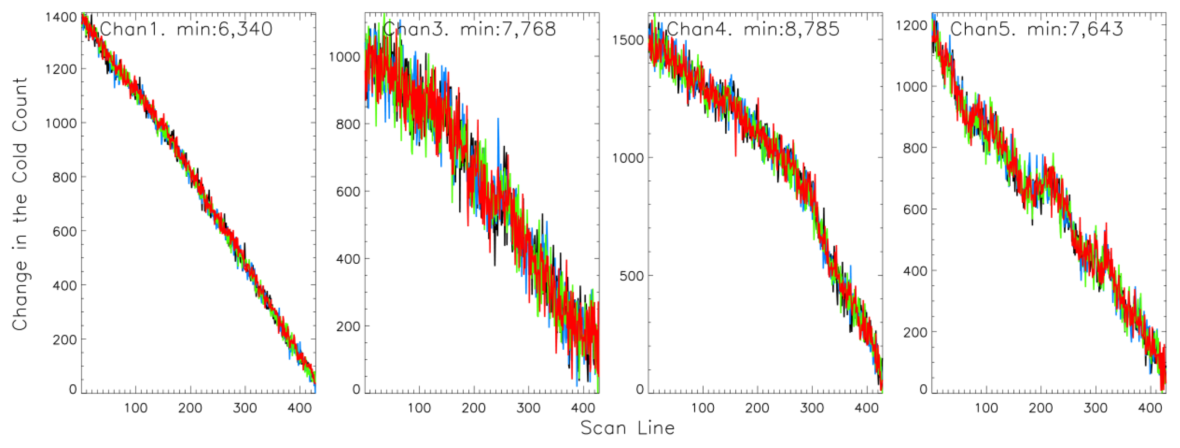
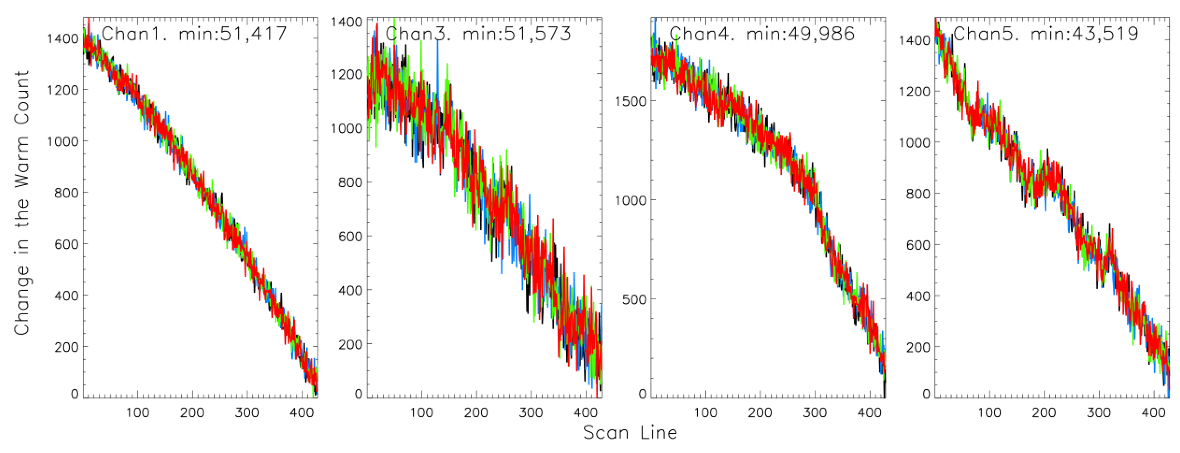
Figure 4 provides a similar analysis but for the MHS instrument. In this case, only the data from the four good channels are included, as channel 2 was declared failed on 26 February 2020. In contrast to AMSU-A’s results, the cold counts and warm counts from the two calibration targets for the MHS exhibited a gradual reduction over time. Like AMSU-A, there was no discernible period of relative stability in the data throughout the test period.
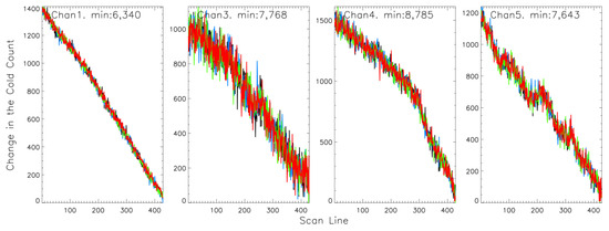
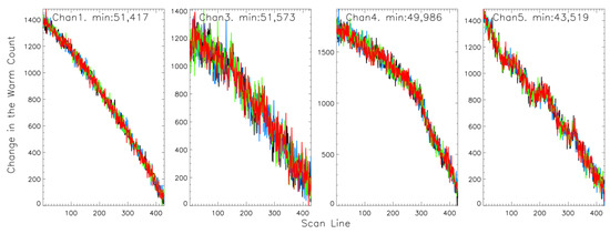
Figure 4.
Cold counts (top panel) and warm counts (bottom panel) from the MHS channels during the DSVT period. Only good MHS channels are shown here. Channel 2 failed (declared on 26 February 2020). Different targets are shown separately using different colors (black for target 1, blue for target 2, green for target 3, and red for target 4). Note that for each channel the y-axis represents the change in the cold (warm) count related to its minimum count during the period.
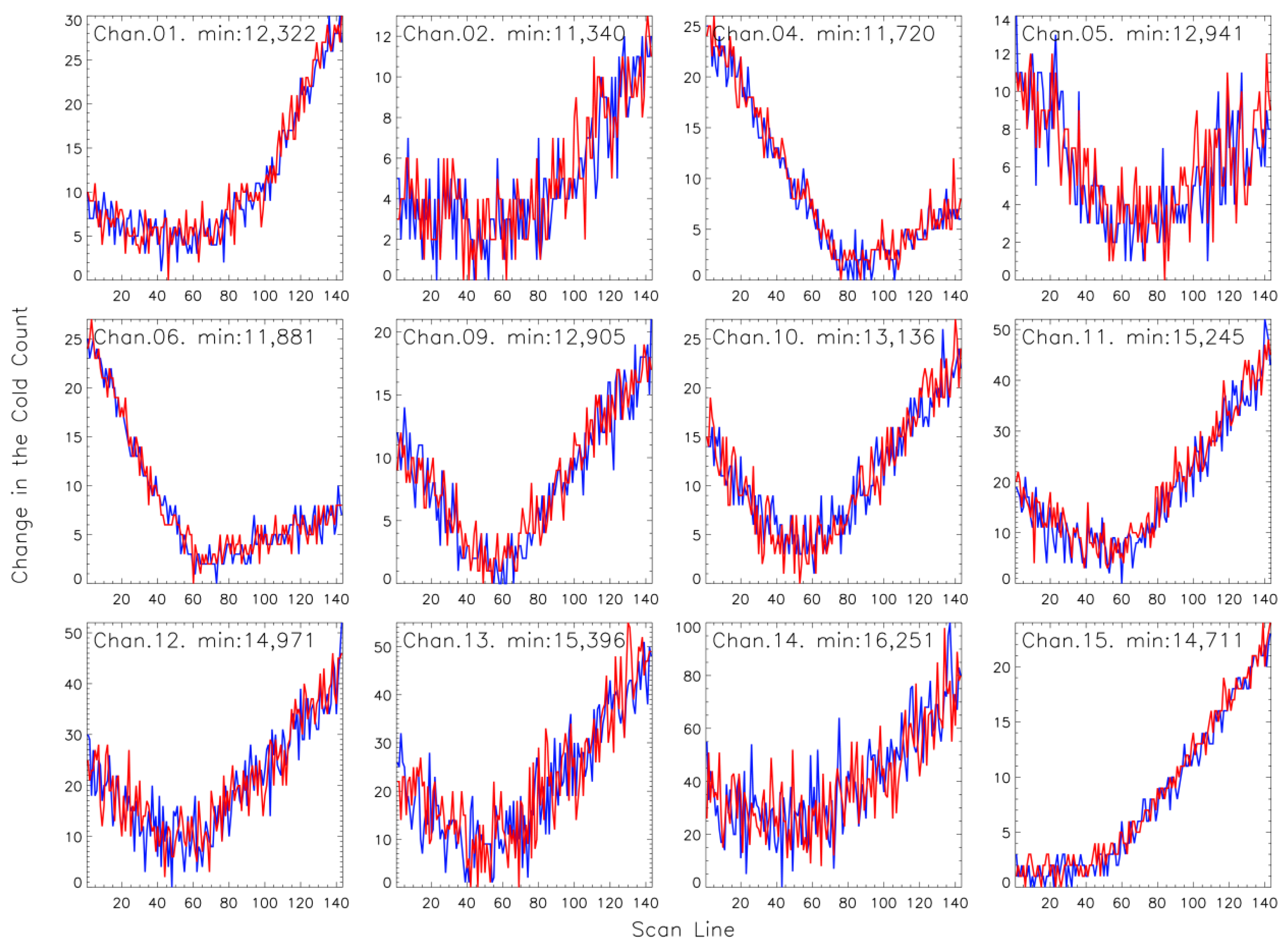
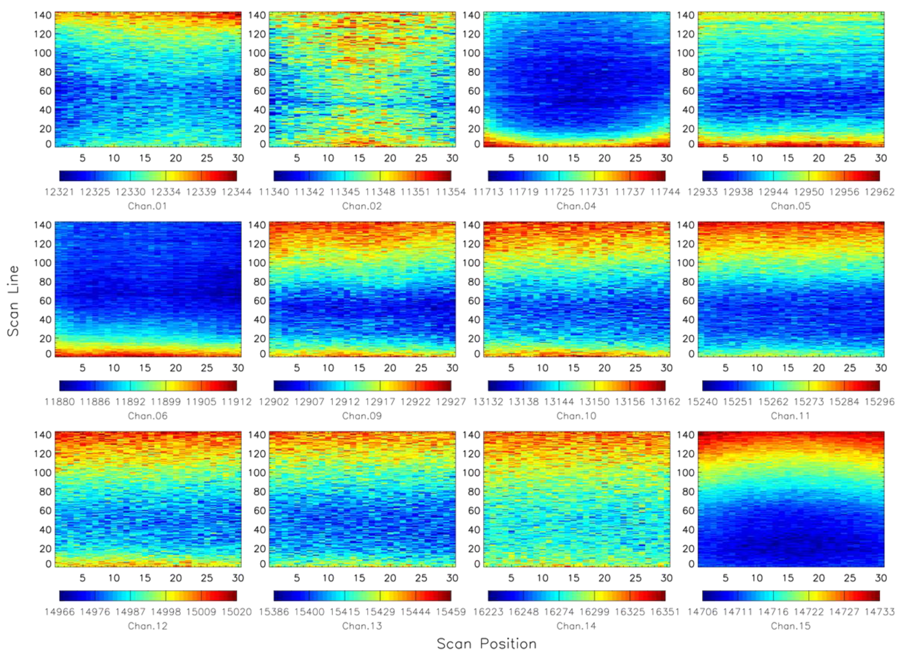
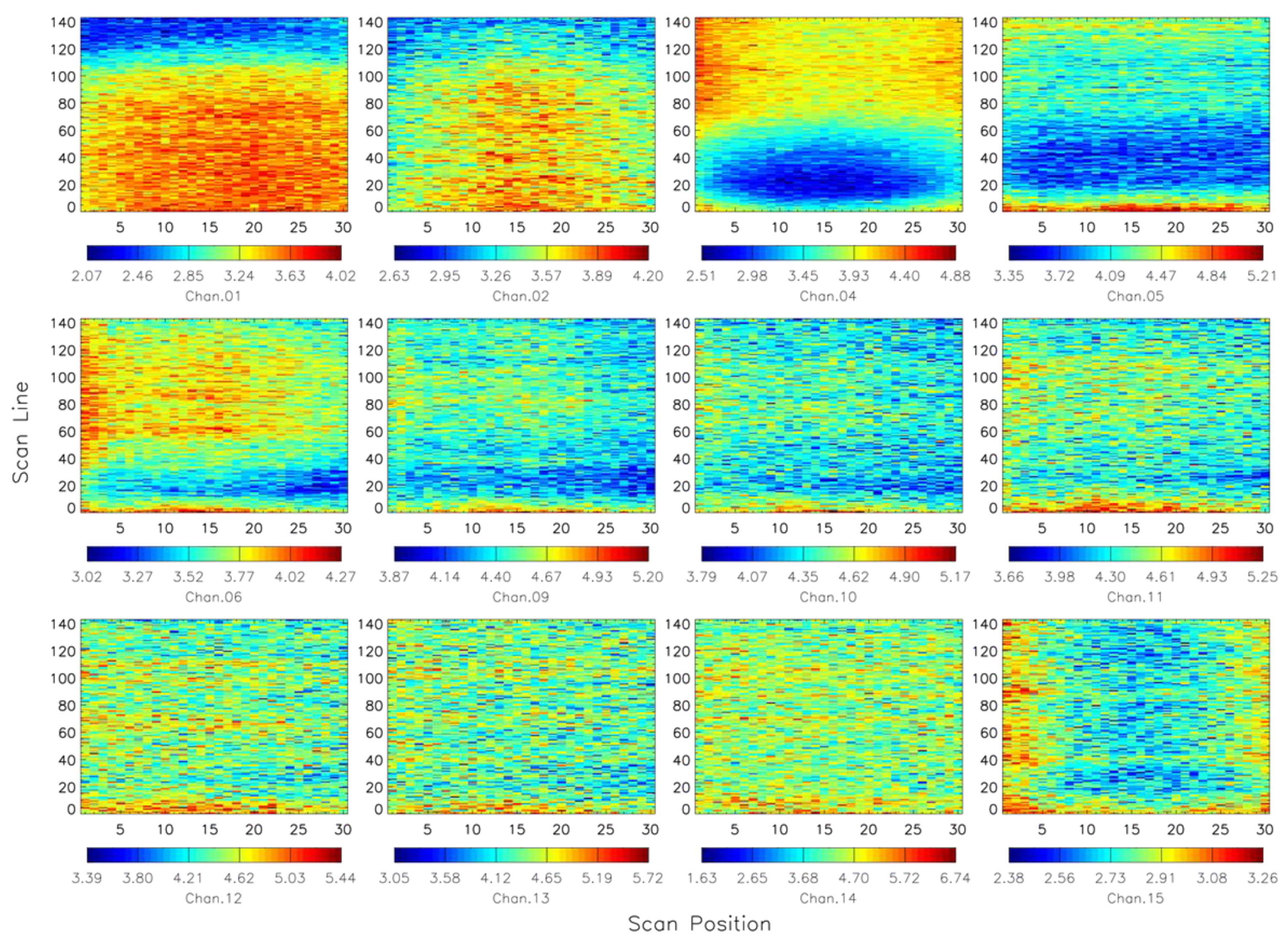
Figure 5 provides a comprehensive visualization of the AMSU-A deep space view (Earth view under normal scan conditions) counts, showing their variation across scan positions (corresponding to the 30 FOVs). What becomes immediately apparent is that the deep space view counts were far from homogeneous throughout the entire test period. There were substantial fluctuations along both the along-track (y-axis) and cross-track (x-axis) dimensions. It is worth highlighting that the count changes along the scan lines (along the track) exhibited a magnitude similar to the cold counts displayed in Figure 2. In principle, if there were no other contributing factors, the counts from the Earth view (deep space view) should ideally match those from the cold view, as both views observed the same deep space with a temperature of 2.728 K (but with different scan view angles).
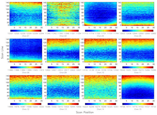
Figure 5.
Scene counts (deep space view) from the AMSU-A channels during the DSVT period. The deep space view counts were not homogeneous during the test period, exhibiting large variations in the along-track and cross-track directions.
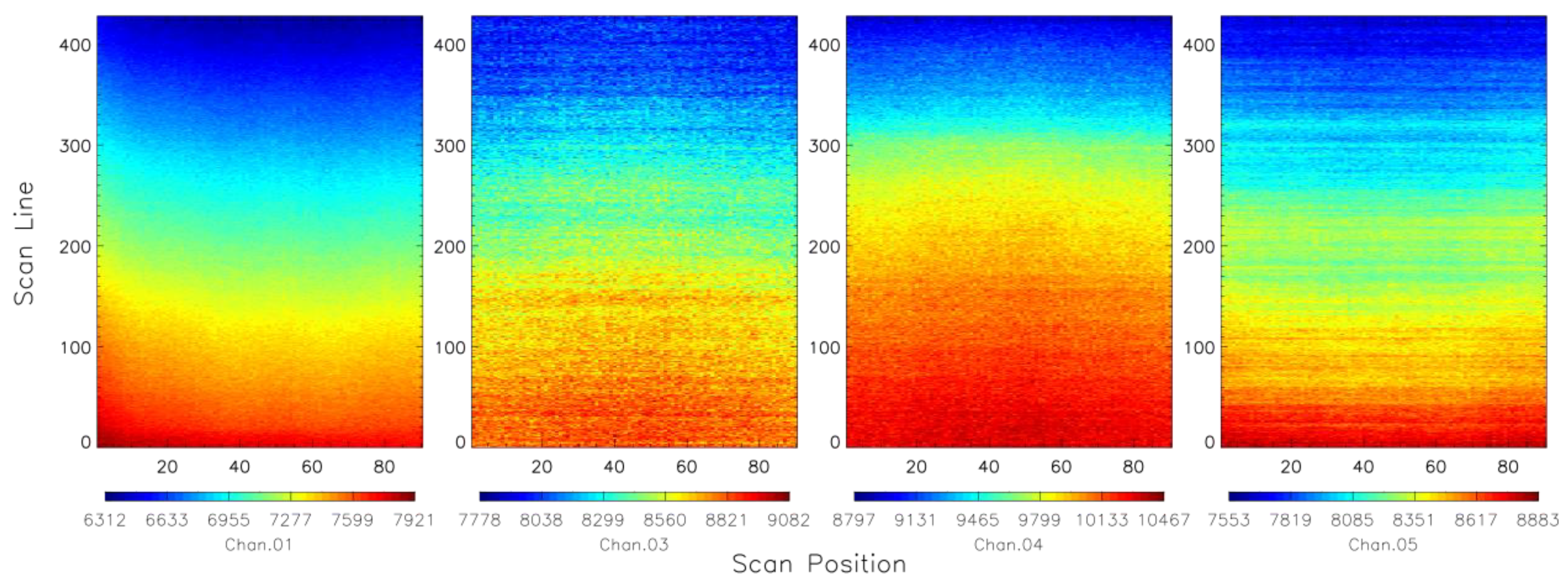
Figure 6 shows the MHS instrument’s deep space view counts change as a function of the scan lines against the scan positions (corresponding to 90 FOVs). Because of the three-times faster scan time and three-times greater number of scan positions in comparison to the AMSU-A, the MHS’s deep space view counts exhibited a smoother change pattern. However, similar to the AMSU-A, these counts also displayed a lack of homogeneity, with substantial variations observed in both the along-track and cross-track directions. Particularly evident is the asymmetrical scan pattern, notably in channel 1, which featured higher values at the starting scan positions.
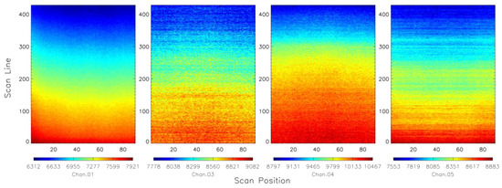
Figure 6.
Scene counts (deep space view) from the MHS channels during the DSVT period. The deep space view counts were not homogeneous during the test period, exhibiting large variation in the along-track and cross-track directions.
These visualizations of the test data provide valuable insight into the behavior of both the AMSU-A and MHS deep space view counts, underscoring their nonuniform nature and highlighting the presence of certain systematic patterns, such as the observed asymmetry in the scan patterns. Understanding and interpreting these variations in the DSVT data collection is crucial for understanding the instruments’ performance characteristics and performing the data analysis.
3. Data Analysis and Results
3.1. Instrument Noise Analysis
We performed noise estimation from the counts of cold targets and warm targets using the Allan deviation method [17,18] to account for the rapid temperature changes. The results show that both the AMSU-A and MHS instruments’ noise was maintained at the same level as under the normal Earth scan conditions. These values of noise equivalent differential temperature (NEΔT) derived from the test period are given in Table 2. They show that the noise values from the cold target views were smaller than those from the warm target views for all of the AMSU-A and MHS channels. Under the normal Earth scan conditions, it is difficult to carry out a noise analysis using the Earth counts due to their natural variability when scanning over different scenes on the Earth. During the space view test, the antenna temperature is very close to the cold target temperature (~2.73 K), it would be expected that the scene noise should be very close to that of the cold targets. This test provides a unique opportunity to prove that. We further performed the noise estimation from the scene counts (deep space view counts in this study). The results show that the noise derived from the scene counts (NEΔTscene) is actually very close to that of the cold targets. The values NEΔTscene presented in Table 2 were derived by averaging over 30 FOVs for the AMSU-A and over 90 FOVs for the MHS during the DSVT test period. As a result, we could use the noise derived from the cold targets to represent the instrument measurement noise in this study. Although the absolute instrument noise (NEΔTcold) was smaller than that of the normal Earth scan conditions (represented by NEΔTwarm, with the scene temperature approximately above 200 K), the relative noise in the observed data (with a scene temperature of ~2.73 K) significantly increased for the deep space view data that were used in this study.
Table 2.
AMSU-A and MHS instrument noise for cold targets, warm targets, and scenes (averaged over 30 FOVs for the AMSU-A and over 90 FOVs for the MHS) during the DSVT test period.
3.2. Antenna Temperature and Brightness Temperature
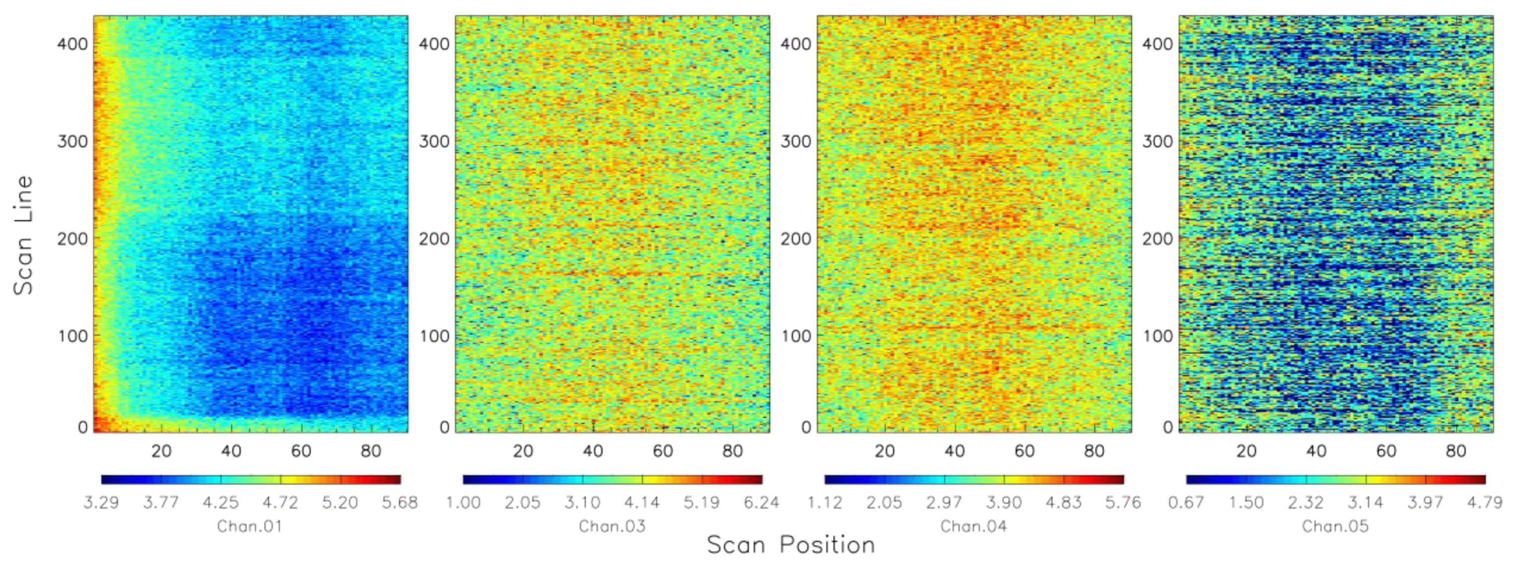
The observed counts from all channels of both the AMSU-A and MHS were converted to the antenna temperature after calibration using the data shown in Section 2. The correction of the cosmic background temperature via Planck’s radiation law was used in the conversion by adding a frequency-dependent correction temperature. The resulting AMSU-A and MHS antenna temperatures, shown as a function of the scan position during the test period, are presented in Figure 7 and Figure 8, respectively. The antenna temperatures derived from deep space views are ideally expected to capture only the microwave radiance emanating from the cosmic background. Consequently, they should exhibit relative cleanliness and stability, with a theoretical value of approximately 2.73 K if there are no other radiance sources. However, the observed deep space view antenna temperatures reveal significant variability and dispersion, both along the cross-track (scan position) and along-track directions for each channel. For example, the antenna temperatures from AMSU-A channel 9 range from 3.87 K to 5.20 K, with no uniform distribution observed along the scan positions. Similarly, the antenna temperatures from MHS channel 1 span a range from 3.29 K to 5.68 K, with the variations also not evenly distributed across the scan positions. Significantly larger along-track variations are observed in the AMSU-A data compared to the MHS data. The notable variations in the AMSU-A antenna temperature data can be attributed to its higher rate of temperature change per scan compared to the MHS, given that the scan time for the AMSU-A is three times longer than that of the MHS (8 s and 8/3 s, respectively). For example, the averaged PRT temperature changes per scan during the test period are −1.05 mk, −1.40 mk, −1.19 mk, and −1.0 mk for the AMSU-A11, AMSU-A12, AMSU-A2, and MHS, respectively (see Figure 1). For the AMSU-A and MHS, the calibration is performed at each scan using the averaged temperatures for the warm calibration target (PRT) and cold calibration target (deep space) from the corresponding scan. The along-track variation observed in the scene BTs does not necessarily indicate that the calibrations are ineffective. Instead, it reflects the dynamic nature of the space view and instrumental conditions during the satellite’s backflip maneuver. It is important to note that despite the periodic calibrations, the rapid temperature changes in the PRTs and fluctuations in the instrument components can still introduce scan-to-scan variations. We want to emphasize that the AMSU-A and MHS calibrations were carefully designed and implemented to guarantee the reliability of these data. While along-track variations may be observed in scene BTs, the aggregated data from the DSVT test remain accurate for their intended purpose in our study. These observations underscore the complexities of achieving precise and stable measurements in the microwave radiance domain, necessitating a careful understanding of instrument characteristics and factors that may influence data quality.

Figure 7.
Scene antenna temperature from AMSU-A channels during the DSVT period as a function of scan positions. The deep space view temperatures were not homogeneous during the test period, exhibiting large variations in the along-track (noise and contaminations) and cross-track (asymmetric scan biases due to antenna sidelobe contributions) directions.
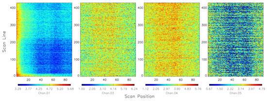
Figure 8.
Scene antenna temperature from the MHS channels during the DSVT period as a function of the scan positions. The deep space view temperatures were not homogeneous during the test period, exhibiting large variations in the along-track (noise and contaminations) and cross-track (asymmetric scan biases due to antenna sidelobe contributions) directions.
To mitigate the along-track variation and enhance the data quality, we averaged the AMSU-A and MHS antenna temperatures using all of the available scan lines obtained during the test period. Figure 9, Figure 10 and Figure 11 show the mean antenna temperatures for the AMSU-A (represented by red dots) as a function of the scan position, while Figure 12 presents the mean antenna temperatures for the MHS (also represented by red dots). These averaged antenna temperatures exhibited notable asymmetry and a strong dependence on scan positions. These characteristics suggest the presence of radiance contributions originating from both the antenna sidelobe and antenna emissions. To address these contributions and refine the data, we applied an antenna pattern correction (APC) to the MetOp-a AMUSA and MHS instruments. This APC primarily accounted for the antenna sidelobe contribution and was derived from the data obtained during the prelaunch thermal vacuum test (TVAC), as referenced in the works of [8,9]. Following [9,16], the brightness temperature, , can be derived from the antenna temperature, , by applying the APC coefficients at the scan position, :
with:
where , , and are the three antenna efficiency values for the Earth, cold space, and satellite platform, respectively. In addition, is the scale factor to account for the approximation of the near-field effect of the satellite platform due to the use of the far-field pattern function data; and are the brightness temperature of the cold space seen by the sidelobes and brightness temperature of the antenna on the satellite, respectively. The value of from the antenna reflector is not measured for the MetOp-A AMSU-A and MHS instruments. It can be replaced by the RF shelf temperature for the AMSU-A and the IF baseplate temperature for the MHS (see Figure 1) that are measured onboard. It is important to clarify that the antenna reflector temperature mentioned here differs from the receiver temperature. Furthermore, it is important to note that the antenna reflector is exposed to the external space environment, whereas the receiver is internal to the instrument shielded from the external radiation, leading to a substantial temperature difference between the two. It is assumed that the APC coefficients remain constant throughout whole mission. With this assumption, we can derive the brightness temperature, effectively removing the contribution from the antenna sidelobe. These steps were crucial for ensuring the accuracy and reliability of the brightness temperature data by correcting for extraneous radiance sources and factors impacting the observations.
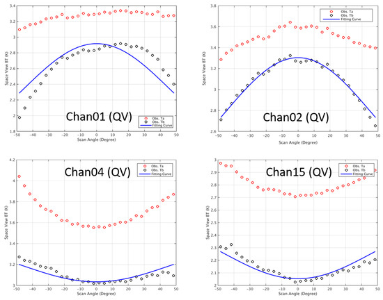
Figure 9.
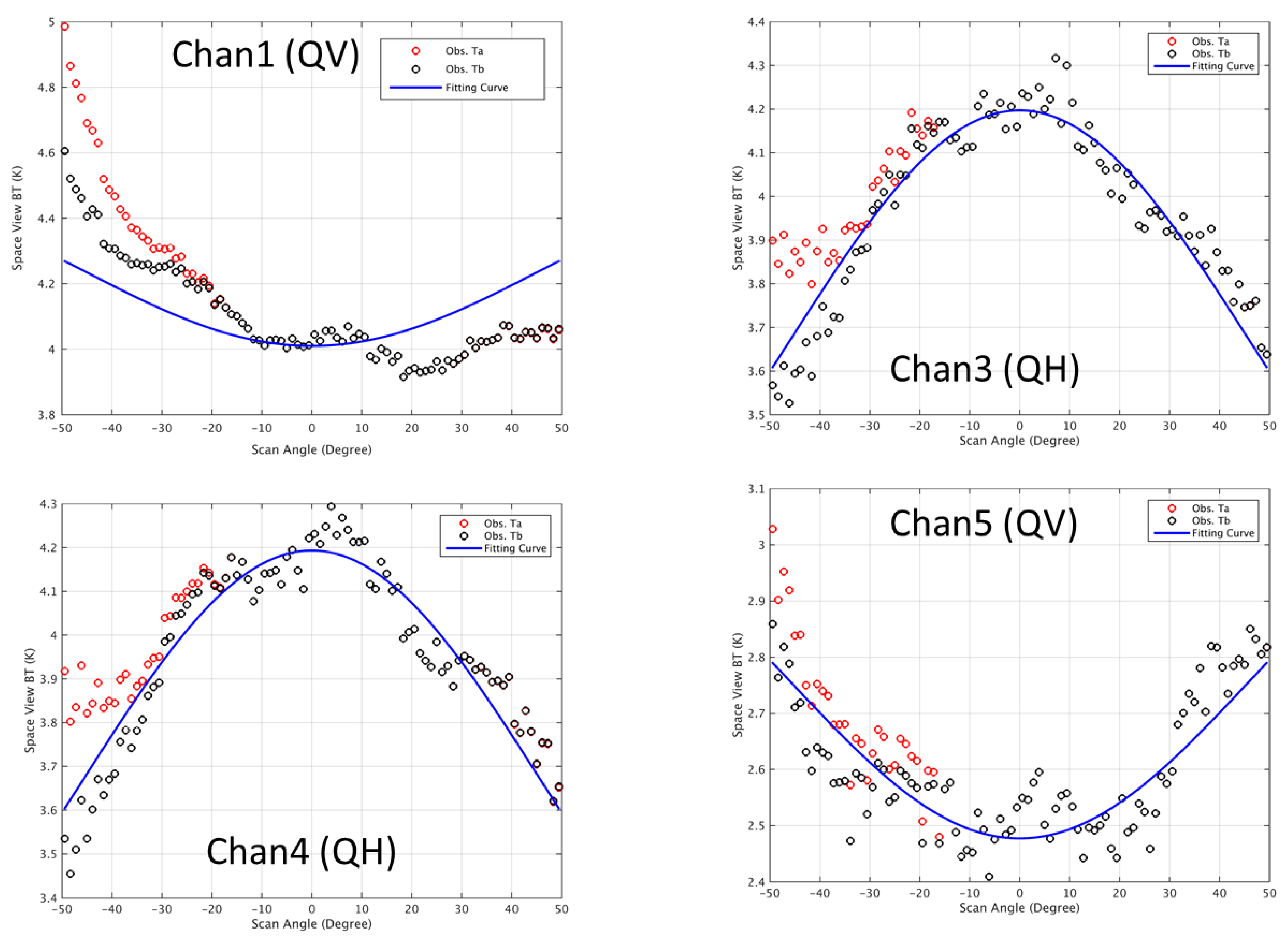
AMSU-A quasi-vertical polarized channels 1, 2, 4, and 15 mean antenna temperature (red dots) and brightness temperature after antenna pattern correction (black dots), as well as the fitting curve (blue line, used to derive the antenna emissivity) versus scan angle. Note that the curve patterns from channels 1 and 2 are different from those from channels 4 and 15. The observed scan-angle-dependent BTs for QV channels 1 and 2 were not expected compared to the emission model.
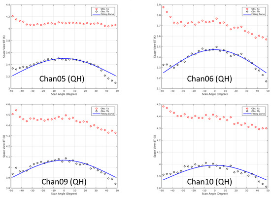
Figure 10.
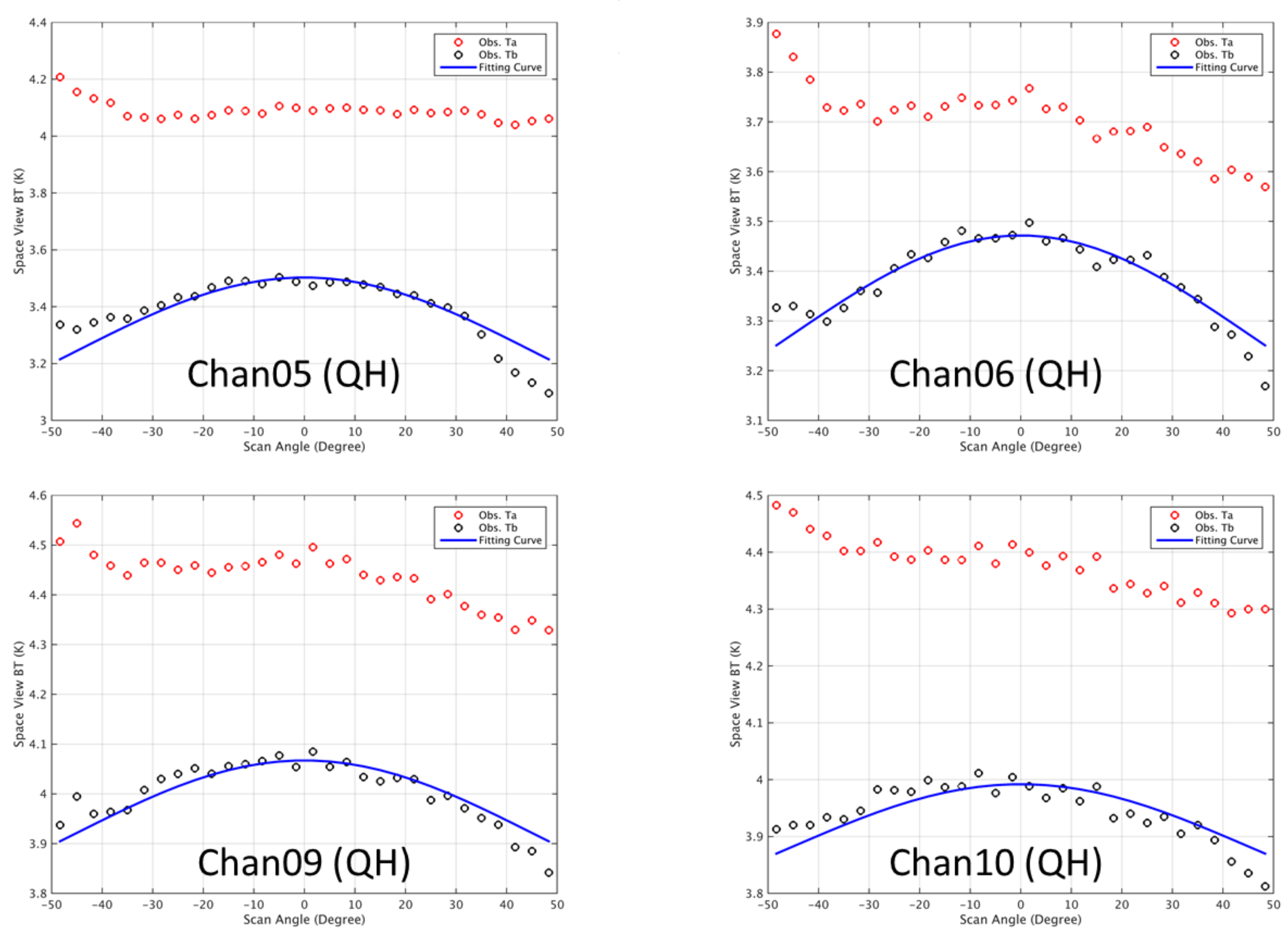
Same as Figure 9 but for the AMSU-A quasi-horizontal polarized channels 5, 6, 9, and 10.
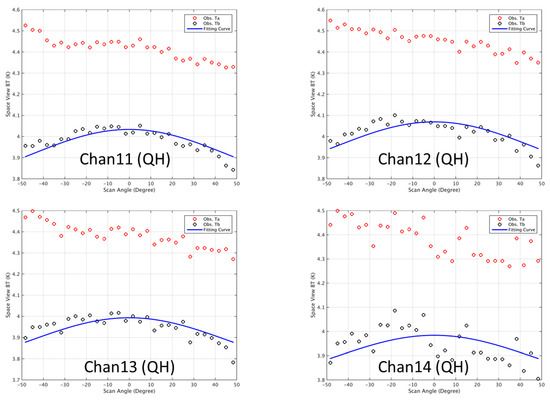
Figure 11.
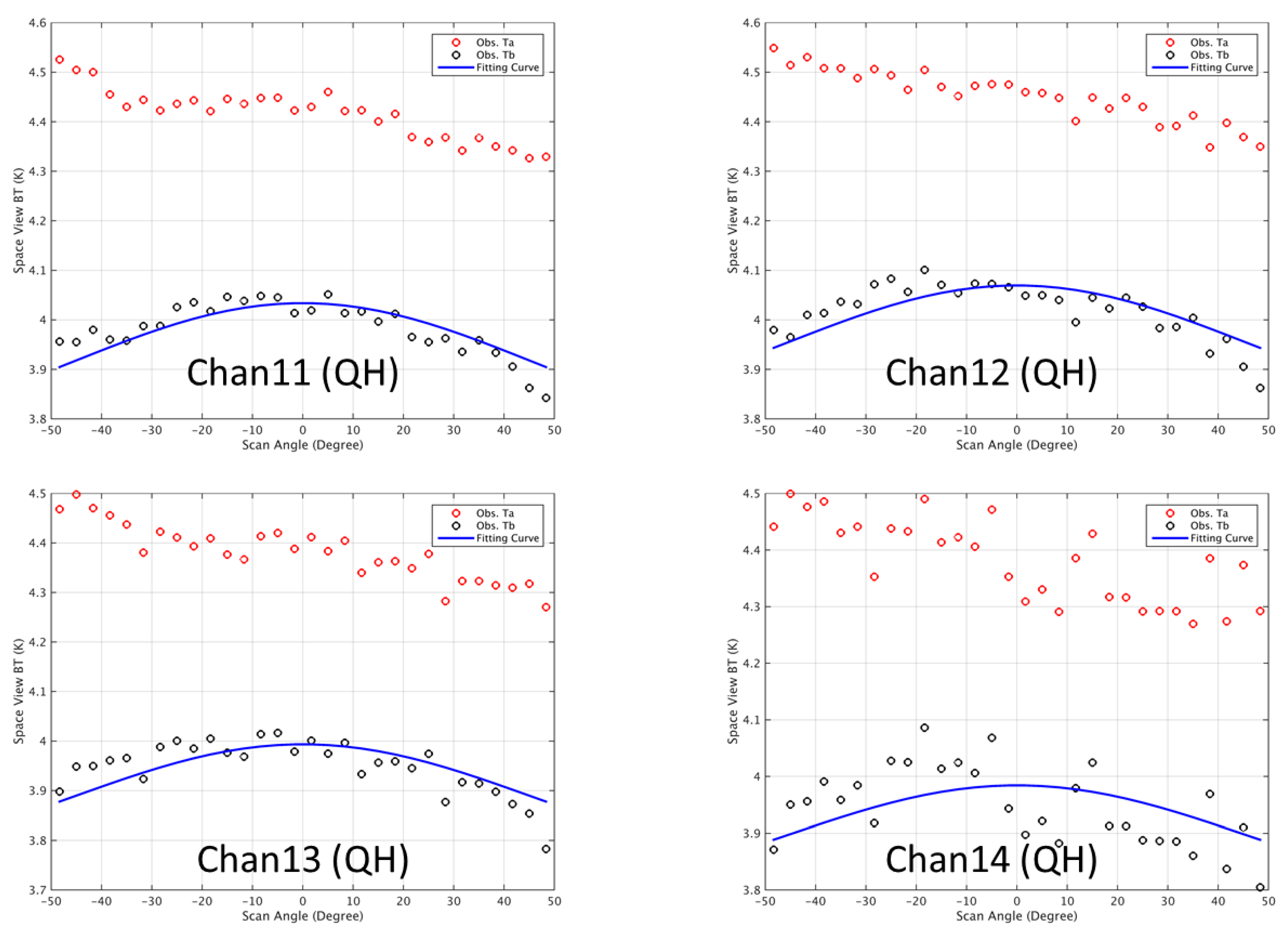
Same as Figure 9 but for the AMSU-A quasi-horizontal polarized channels 11–14.
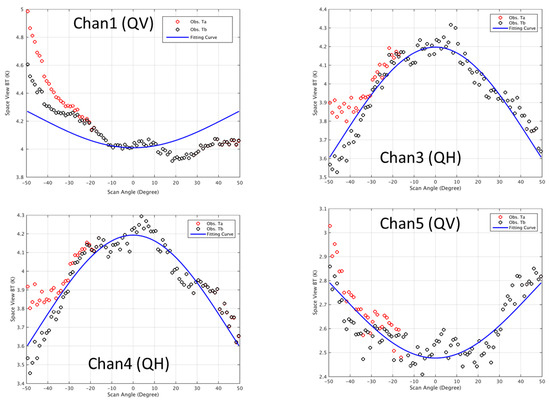
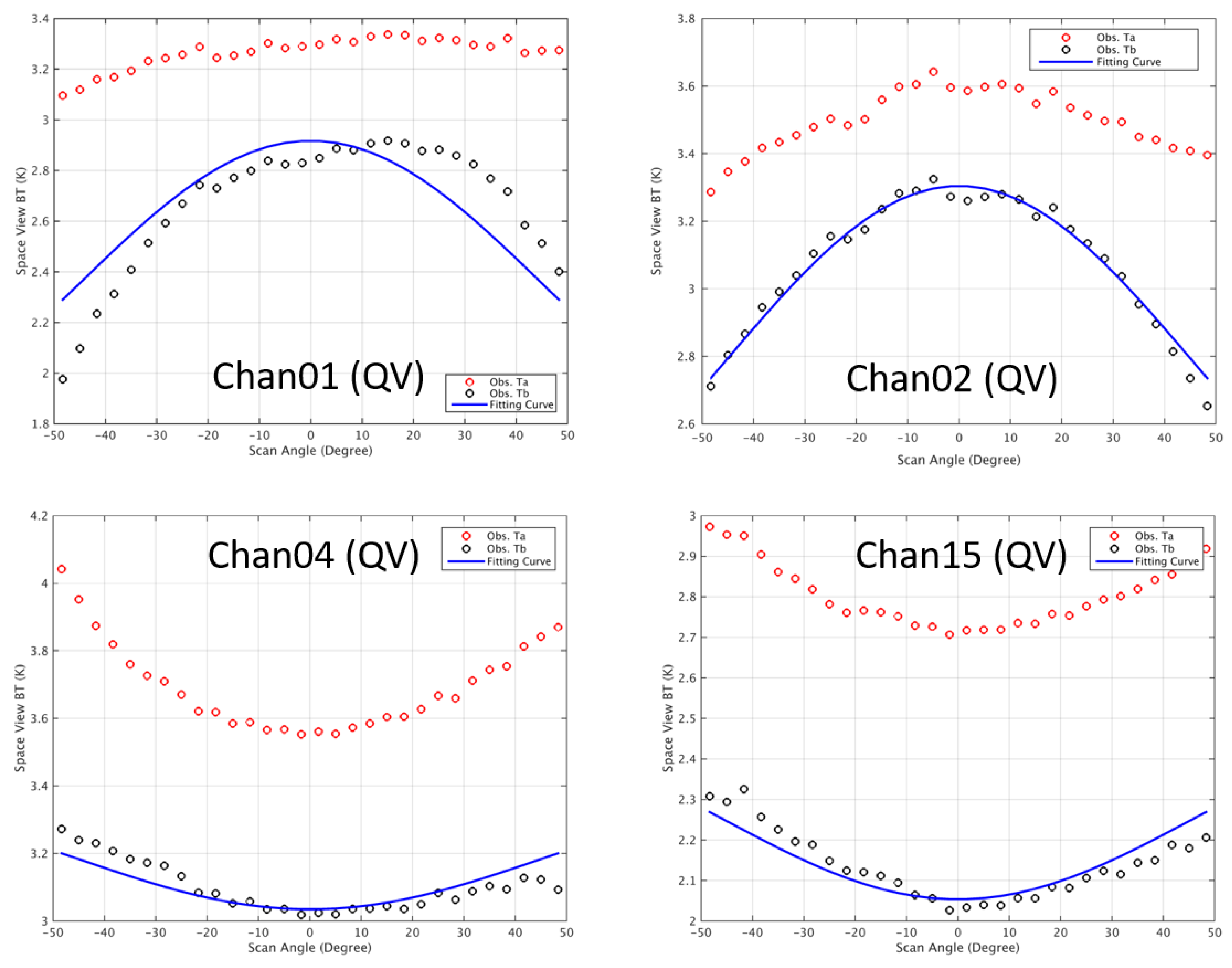
Figure 12.
MHS channels 1, 3, 4, and 5 mean antenna temperature (red dots) and brightness temperature after antenna pattern correction (black dots), as well as the fitting curve (blue line, used to derive the antenna emissivity) versus scan angle. At a given scan angle, when only Tb is present without Ta, this indicates that the observed Ta has the same value as Tb at that specific scan angle with zero sidelobe contribution from the satellite platform.
The brightness temperatures after the antenna pattern correction (indicated by the black dots) versus the scan position derived from the DSVT observations are shown in Figure 9, Figure 10 and Figure 11 for the AMSU-A channels. Similarly, Figure 12 presents the corresponding brightness temperatures for the MHS channels. Following the antenna pattern correction, a noticeable change is evident in the pattern of the brightness temperatures in relation to the scan positions. The previous asymmetrical patterns from the antenna temperatures are significantly reduced, indicating the effectiveness of the antenna pattern correction. However, there is still a discernible scan-angle-dependent feature presented in the data. These remaining variations underscore the complex nature of the radiance measurements from the microwave instrument and the importance of continued analysis to understand the extraneous radiance sources.
3.3. Antenna Emissivity Estimated from Observations
The fundamental expectation is that the brightness temperatures from deep space views, once calibrated against the cold space, should exhibit uniformity across the entire scan range. However, the observed scan-angle-dependent BT suggests that additional factors are at play here. Contributions from the near-field radiation emanating from the satellite platform and the instrument itself may be responsible for this observed variation. Prior research efforts, as documented in the studies in [12,13], have sought to address this issue. They established a model to derive antenna emissivity using deep space view test data from the ATMS on the SNPP. This model was instrumental in explaining the scan-angle-dependent feature observed in the ATMS measurement bias. By considering the effects of the antenna emissivity, such research endeavors aim to provide a more comprehensive understanding of the microwave radiance measurement uncertainty and contribute to the refinement of the data calibration processes. Following [13], the quasi-vertical (QV) and quasi-horizontal (QH) polarized corrections are expressed as a function of the scan angle:
where is the scan angle, and and are the model parameters determined from the deep space view test data. Based on this model, at the nadir (directly above the satellite in the deep space view test), the observed brightness temperatures should have a minimum at all QV channels and a maximum at all QH channels. However, when we examine the results presented in Figure 9, it becomes apparent that the brightness temperatures from channels 1 and 2 do not exhibit the expected sine-squared shape of the scan-angle-dependent variation. Instead, they show a maximum at the nadir, which contradicts the model’s prediction. In contrast, for all other channels, the scan-angle-dependent features of the brightness temperatures for both the QV and QH polarizations, predicted by the model, align with the observations from the DSVT. This discrepancy suggests that there may be specific characteristics or factors influencing channels 1 and 2 that are not entirely captured by the existing model. Further investigation of the possible reasons may be necessary to fully understand and reconcile these observations with the expected behavior.
The model parameters and are a function of the emissivity and physical temperature of the reflector:
The reflector emissivity for QV () and QH () can be derived by:
where , and are the radiance from the calibration blackbody target, cold space, and the antenna reflector, respectively. , , and are the scan angles for the warm load, cold space, and “Earth scene”, respectively. is the ratio between the difference from the scene count and cold space count and the difference from the warm load count and cold space count. Note that the retrieved H-pol emissivity should be used for the QV channels and the V-pol emissivity for the QH channels, since the reflector emissivity is defined with respect to the reflector scanning plane, which is different from the Earth surface scattering plane in which the instrument polarization is defined.
The model fitting results for the brightness temperature of the AMSU-A channel are presented in Figure 9, Figure 10 and Figure 11. Figure 9 displays the mean antenna temperature (red dots) and the brightness temperature after the antenna pattern correction (black dots) for the AMSU-A QV channels 1, 2, 4, and 15. This also includes a fitting curve (blue line) that is used to derive the antenna emissivity. Importantly, the curve patterns for channels 1 and 2 differ from those observed for channels 4 and 15. Notably, the scan-angle-dependent BTs for QV channels 1 and 2 do not align with the expectation based on the emission model, indicating unexpected behavior. Figure 10 presents the results for the AMSU-A QH channels 5, 6, 9, and 10, offering a view of the mean antenna temperature, BT after antenna pattern correction, and the fitting curve specific to these channels. The fitting curve closely tracks the BT data for scan positions 6 to 25, with a smaller value at the starting edge positions (1–5) and a larger value at the ending edge positions (26–30). This pattern suggests that the fitting curve effectively captures the scan-angle-dependent feature of the BT data within the central portion of the scan range, aligning well with the observations. However, the deviations at the scan edges indicate that there may be additional factors or characteristics influencing the measurements in these regions. Figure 11 continues the analysis for the AMSU-A QH channels but focuses on channels 11 through 14. It provides a comprehensive view of the mean antenna temperature, BT after antenna pattern correction, and the corresponding fitting curve for these channels. The alignment of the fitting curves with the BT data is similar across the channels, as observed in Figure 10. However, it is noted that for channel 14, there appears to be less alignment between the fitting curve and the BT data, indicating a greater discrepancy between the model and the observed measurements.
The retrieved reflector emissivity value for each AMSU-A channel used the fitting data rather than the real measurement that is given in Table 3. It is notable that channels 1 and 2 have negative values, and this deviation from the expectation is attributed to the inconsistent pattern between the actual measurements and the model predictions. The AMSU-A channels 9–14 have the same polarization and frequency; in principle, they should have identical retrieved reflector emissivity values. However, the actual retrieved values differ among them. For instance, channel 9 has a value of 0.001, whereas channel 14 has a value of 0.0006. This discrepancy may be attributed to factors such as the presence of significant noise in the observations from channel 9 to channel 14 (from 0.115 K to 0.542 K) compared to the space view temperature of around ~2.73 K (see Table 2), which could contribute to the variations in the derived emissivity values for channels 9 to 14. The significant noise and rapid instrument temperature changes and their impacts on the derived emissivity values highlight the challenges in the precise radiance measurements and the need to carefully account for such factors in the calibration and correction processes.
Table 3.
Retrieved antenna reflector emissivity at the AMSU-A channels. Note that the negative values for channels 1 and 2 are due to the inconsistent pattern between observation and model prediction.
The model fitting results for the MHS channel brightness temperature are shown in Figure 12. It presents all of MHS channels 1, 3, 4, and 5 mean antenna temperatures (red dots) and brightness temperatures after antenna pattern corrections (black dots), as well as the fitting curve (blue line, used to derive the antenna emissivity) as a function of the scan angle. There are some variations in how different channels respond to the correction process. Specifically, after the antenna pattern correction, channel 1 continues to exhibit significant asymmetrical scan biases, whereas channels 3, 4, and 5 show improvements. This observation suggests that the effectiveness of the antenna pattern correction may vary among channels, and in the case of channel 1, the correction might not be as effective as desired. Further refinements in the antenna pattern correction for channel 1 may be necessary to achieve the desired calibration accuracy and consistency across all MHS channels.
The retrieved reflector emissivity values presented in Table 4 were determined using fitting data rather than real measurements for the MHS channels. These emissivity values provide insight into the behavior of the MHS channels after correction and calibration. It is noteworthy that the emissivity values align with expectations and theoretical considerations. In particular, the emissivity values for channels 1, 3, 4, and 5 are as follows: 0.0016, 0.0036, 0.0036, and 0.0019, respectively. It is worth noting that channels 3 and 4 have the same emissivity (0.0036) because they share the same center frequency. Furthermore, the emissivity values for channels 3 and 4 are approximately double compared to channel 5 (0.0019). This difference is attributed to the polarization characteristics of these channels, where channels 3 and 4 have horizontal polarization, while channel 5 has vertical polarization (QV). These results align with expectations based on theoretical considerations (Equation (7)) and support the understanding that antenna emissivity values for QH channels should be greater than those for QV channels. This consistency validates the calibration and correction procedures applied to the MHS instrument and enhances confidence in the accuracy of the derived emissivity values. Furthermore, it is also noteworthy that the antenna emissivity values for AMSU-A channel 15 and MHS channel 1 are very similar (0.0014 vs. 0.0016), given that they operate at the same frequency and polarization. This similarity in the derived antenna emissivity values between the two instruments is an important validation point and contributes to the overall trustworthiness of the procedures used in this study.
Table 4.
Retrieved antenna reflector emissivity at MHS channels.
3.4. AMSU-A Channels 1 and 2 QV or QH Polarization?
The scan-angle-dependent brightness temperature from DSVT measurements for channels 1 and 2 after antenna pattern correction are a cosine-squared function of scan angle (frown shape), similar to the patterns from the QH-polarized channels, which contradicts to the instrument design specification of QV channels. The empirical model cannot be applied to these two channels, as a result, the derived reflector emissivity values are negative value from observations. This discrepancy raises the natural question: could channels 1 and 2 actually be QH-polarized channels?
To investigate this issue, simulations were conducted using the Community Radiative Transfer Model (CRTM) [19]. A pseudo instrument similar to the AMSU-A on MetOp-A, but with QH polarization for channels 1 and 2, was generated. Clear sky radiance simulations were performed using forecast data from the European Centre for Medium-Range Weather Forecasts (ECMWF) as input to the CRTM on 5 September 2021. Subsequently, the observation minus background simulation (O−B) difference was analyzed to assess the consistency of the data. This approach allows for a systematic examination of whether channels 1 and 2, indeed, exhibit QH polarization characteristics, as indicated by the observed brightness temperature patterns.
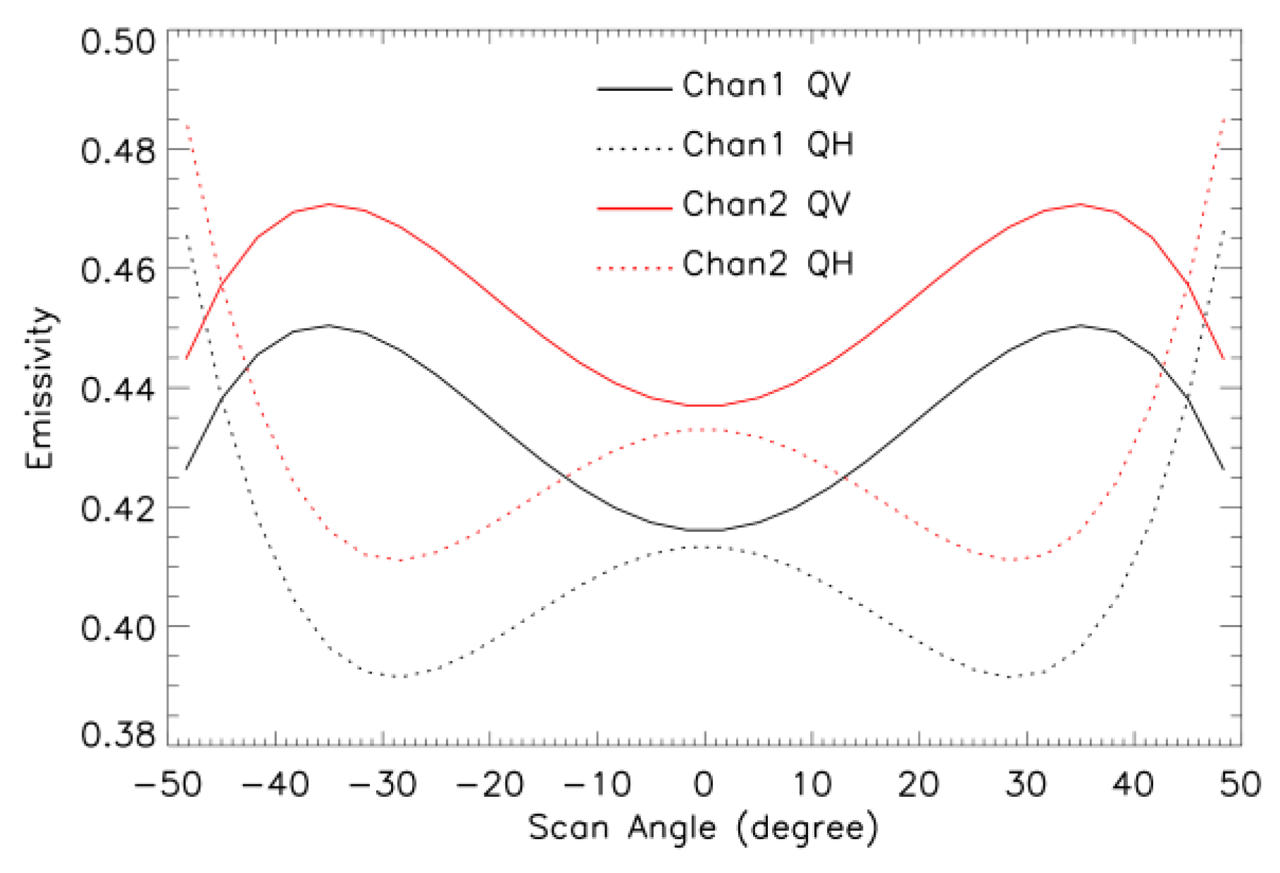
Figure 13 shows the simulated sea surface emissivity for AMSU-A channels 1 and 2 at QV (solid lines) and QH (dashed lines). Within the scan angle [−45, 45], the emissivity values for the QV are consistently greater than those for the QH. Moreover, significant differences in the emissivity are observed at specific scan angles, particularly in the range from 20 to 40 degrees and their corresponding negative angles from −20 to −40 degrees. These differences can be substantial, reaching up to 0.07.
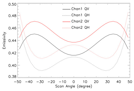
Figure 13.
Simulated sea surface emissivity for the AMSU-A channels 1 and 2 at the QV (solid lines) and QH (dashed lines). Large emissivity differences exist at scan angles from 20 to 40 degree (and −20 to −40 degree).
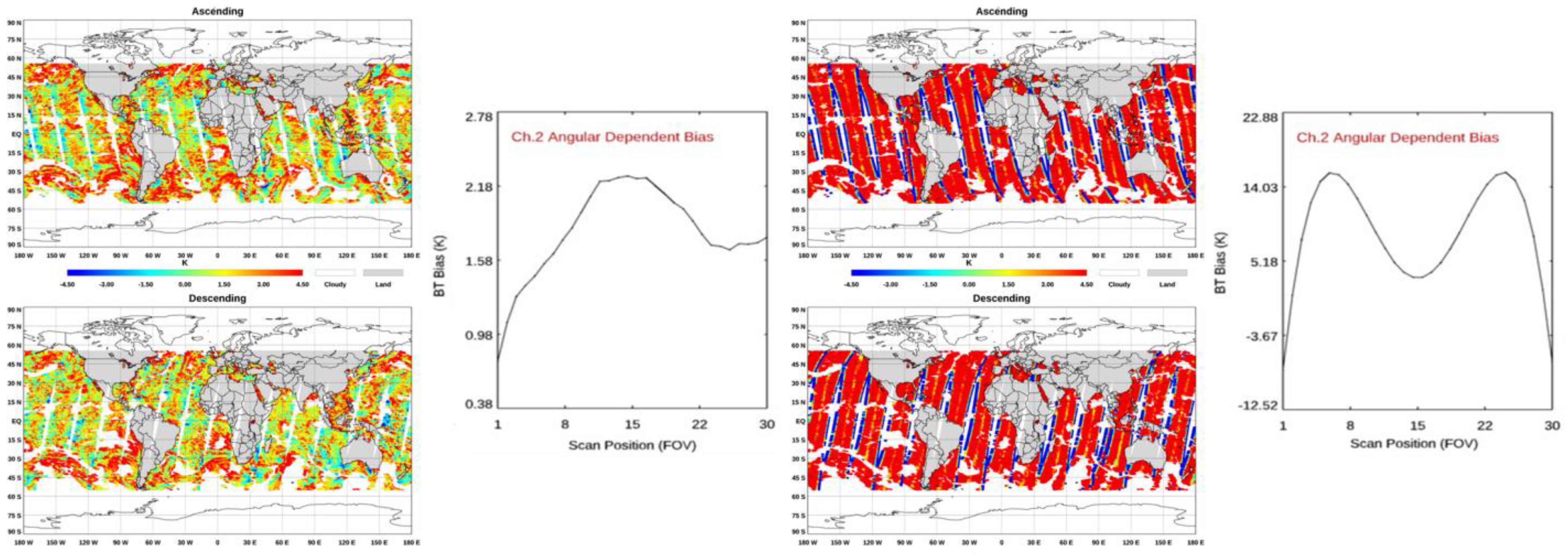
Figure 14 provides a comprehensive comparison between the AMSU-A channel 1’s global brightness temperature differences between observations and simulations over clear oceans and the corresponding mean angular-dependent biases. The left panel corresponds to the QV polarization, while the right panel corresponds to the QH polarization.
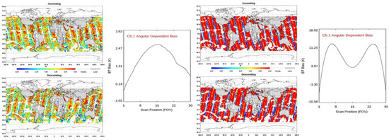
Figure 14.
AMSU-A channel 1 global brightness temperature difference between observation and simulation over clear oceans, as well as the mean angular dependent bias: (left) QV polarization and (right) QH polarization. It clearly shows that AMSU-A channel 1 is QV polarization with a reasonable difference between observation and simulation.
Key observations from this comparison are as follows:
- (1)
- The global differences (O−B differences) for the QV polarization remain within a very reasonable range, spanning from −4.5 K to 4.5 K. This range suggests a good agreement between the observed and simulated data.
- (2)
- In contrast, the differences for the QH polarization significantly exceed this range, indicating a substantial discrepancy between observation and simulation. Furthermore, the mean angular-dependent bias shows a distinct double-peak pattern near a scan angle of ±35 degrees, corresponding to the regions of larger sea surface emissivity differences between the QV and QH polarization (as shown in Figure 13).
- (3)
- The clear disparity in the O−B differences between the QV and QH polarization supports the conclusion that the AMSU-A channel 1 is, indeed, quasi-vertical polarized, consistent with the instrument’s design specification.
Similar results were obtained for channel 2, as indicated in Figure 15. While the emissivity for channels 1 and 2 at the QV polarization is minimal at a zero-degree scan angle compared to other angles (Figure 13), it is not essential for the O−B bias, as a function of the scan angle, to exhibit a “dip” (minimum) at zero degrees (between scan positions 15 and 16). This lack of dip can be attributed to significant atmospheric contributions from water vapor emission to the observations from these channels, resulting in distinct shapes between angular-dependent biases and sea surface emissivities. This comprehensive comparison reinforces the assertion that both AMSU-A channels 1 and 2 are quasi-vertical polarized channels, aligning with their designated instrument specifications. These findings provide valuable insight into the polarization characteristics of these channels and contribute to the accurate interpretation of radiometric data obtained from the AMSU-A.

Figure 15.
AMSU-A channel 2 global brightness temperature difference between observation and simulation over clear oceans, as well as the mean angular dependent bias: (left) QV polarization and (right) QH polarization. It clearly shows that AMSU-A channel 2 is QV polarization with reasonable difference between observation and simulation.
4. Discussion
In this study, we conducted an analysis of the MetOp-A AMSU-A and MHS End-of-Life Deep Space View Test data recorded on 27 November 2021. To derive antenna emissivity from the DSVT data, we must rely on some important assumptions. One of the assumptions is that the cold space temperature correction is correct during the backflip maneuver. In operational calibration, a channel-dependent cold space temperature correction is applied, accounting for contamination from radiations originating from the spacecraft platform and Earth’s limb. However, it is crucial to note that the operational cold space temperature correction may not be valid for the flight configuration during the backflip maneuver. The drastic change in viewing geometry during the maneuver may result in different contributions from the Earth’s limb, potentially impacting the radiometric calibration of observations. Unfortunately, we were unable to utilize the DSVT data to derive the cold space temperature correction for each channel due to a lack of necessary measurements in this test. The analyses performed in this study were as follows:
- (1)
- Antenna Pattern Correction: We initiated the analysis by applying the deep space scene antenna temperatures to perform antenna pattern correction on the DSVT data. This correction process was crucial for improving the data’s accuracy and ensuring its reliability. We assumed that these APC coefficients derived from the prelaunch thermal vacuum test data remain constant throughout whole mission. Without this assumption, it is impossible to derive the antenna emissivity from the deep space view test.
- (2)
- Derivation of Antenna Reflector Emissivity Values: Following the APC correction, we proceeded to derive the antenna reflector channel emissivity based on the corrected brightness temperatures. This step was fundamental in characterizing the instrument’s performance and understanding its radiometric behavior.
- (3)
- Variability in Deep Space View Counts: Throughout the study, we noted that the deep space view counts exhibited variability during the test period, particularly with significant variations in both the along-track and cross-track directions. This variability was attributed in part to the rapid and significant change in the instrument temperatures, which impacted the data quality and limited the test’s utility. The temperature did not stabilize for this test. For future DSVT tests of the MetOp series, it is advisable to extend the test duration to ensure temperature stabilization and enhance the accuracy of the space view measurements.
- (4)
- Noise Impact on the Results: The presence of relative substantial noise in the deep space view observations and its negative influence on the data quality were noted. The measurement noise derived from the warm and cold targets for each channel was kept at the same level as under the normal Earth scan conditions. However, considering the low space view antenna temperature of approximately 2.73 K, the noise levels are very significant in a relative sense, and they have a pronounced effect on the data quality, consequently limiting the test’s utility. This noise factor was identified as a potential contributor to the variations in derived emissivity values in channels 9 to 14 with the same frequency.
- (5)
- Scan Pattern after Sidelobe Correction: The scan angle dependent pattern was significantly reduced, although the scene (space view) BTs after sidelobe correction still exhibited a scan-angle-dependent pattern due to the significant contributions of the antenna emissions. Additionally, certain channels displayed an asymmetrical pattern relative to the scan angle. On the basis of our analysis, this asymmetry may be associated with the polarization “twist angle” [20], which can be derived from the emission model by introducing an additional angle, to the scan angle:The inclusion of this “twist angle” allows for a reasonable fit of the scene BTs after sidelobe correction, while maintaining a consistent derived emissivity compared to scenarios where this twist angle is not taken into account. However, for the purposes of this study, we will not incorporate the polarization twist angle, as our analysis indicates that it does not influence the derived antenna emissivity. Figure 16 shows an example with (left panel) and without (right panel) considering the polarization twist angle in the fitting to the observations after sidelobe correction for channel 13.
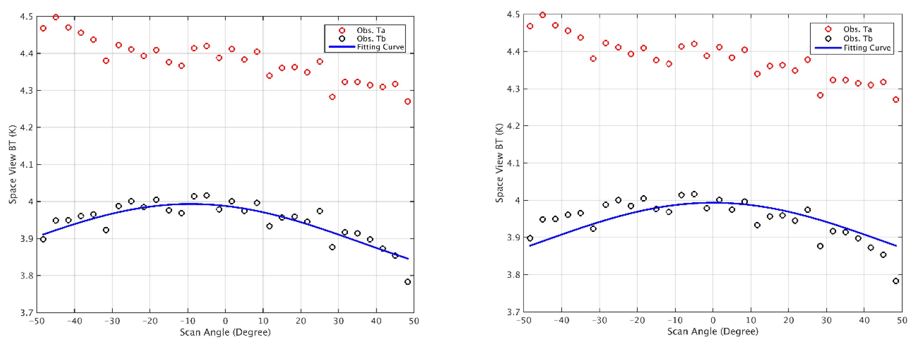
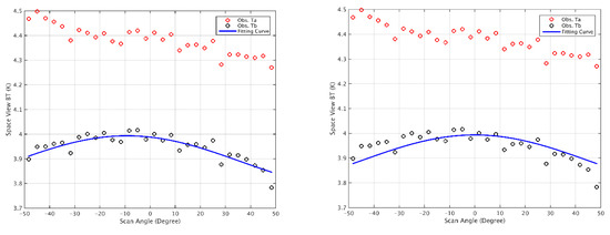 Figure 16. AMSU-A quasi-horizontal polarized channel 13 mean antenna temperature (red dots) and brightness temperature after antenna pattern correction (black dots), as well as the fitting curve (blue line, used to derive the antenna emissivity) versus scan angle: (left) considering polarization twist angle in the fitting curve; (right) without considering the polarization twist angle in the fitting curve. The derived emissivity is 7.4304 × 10⁻⁴ for both cases, and the polarization twist angle is 9.2°.
 - (6)
- Polarization Assessment: The observed scan-angle-dependent brightness temperature behavior for QV channels 1 and 2 after the antenna pattern correction was unexpected and raised questions about their polarization characteristics. However, investigations and simulations confirmed that channels 1 and 2 are, indeed, QV channels as originally designed. The scan bias pattern derived from the DSVT data after sidelobe correction for these channels appears unphysical. The Earth’s limb radiations during the backflip maneuver, coming from the back lobe, may have a relatively small impact on the cold space temperature correction compared to that from the AMSU-A2 normal deep space view observations. However, because of a lack of necessary measurements in the DSVT data, we were unable to derive a new cold space temperature correction to use in the radiometric calibration for the scene BTs during the DSVT test for the AMSU-A2 channels (Earth surface sensitivity channels). This limitation may adversely affect the accuracy of the calibrated scene BTs due to the absence of a corrected cold space temperature. It is important to note that other factors, such as the stability of individual instrument components (including detectors and electronics) and sensitivity to external radiation sources, may also contribute to fluctuations in scene brightness temperatures. These factors could lead to unphysical retrievals for antenna emissivity. Nevertheless, notably, the negative (unphysical) emissivity values retrieved for channels 1 and 2 are not a result of the method used in this study.
5. Conclusions
In this study, MetOp-A AMSU-A and MHS End-of-Life DSVT data on 27 November 2021 were analyzed. The deep space scene antenna temperatures were first applied for the antenna pattern correction, then the antenna reflector channel emissivity values were derived from the corrected temperatures. This study yielded valuable insight into the behavior and characteristics of the MetOp-A AMSU-A and MHS instruments during the EOL DSVT. The study’s primary focus was on determining the actual polarized antenna emission by utilizing on-orbit pitch-over maneuvers.
For the AMSU-A, the deep space view counts exhibited nonuniformity during the test period, displaying significant variations in the along-track and cross-track directions. This variation was primarily attributed to rapid changes in the instrument temperature during the test period. The substantial relative noise observed in the deep space view negatively impacted the data quality, thereby limiting the utility of this test. The large relative noise may contribute to the different emissivity values derived from the same frequency for channels 9 to 14. Additionally, we observed an unexpected scan-angle-dependent BT pattern after antenna pattern correction for quasi-vertical (QV) channels 1 and 2, compared to the emission model. Further investigation using a simulation confirmed that channels 1 and 2, indeed, function as QV channels, as designed.
For the MetOp-A MHS, the antenna pattern correction significantly improved the behavior of brightness temperatures for all channels, except channel 1. The derived antenna reflector emissivity values were found to be 0.0016, 0.0036, 0.0036, and 0.0019 for channels 1, 3, 4, and 5, respectively.
The MHS channels 3 and 4 had the same emissivities, and are approximately twice as large than that from channel 5, which aligns with expectations based on theoretical considerations and enhances confidence in the accuracy of the derived emissivity values. The antenna emissivity values for AMSU-A channel 15 and MHS channel 1 are very similar, which contributes to the overall trustworthiness of the procedures used in this study.
The overarching objective of these efforts is to enhance the quality and accuracy of the NRT products for both the MetOp-B and MetOp-C satellites. Additionally, the study aims to contribute to the overall improvement of the Fundamental Climate Data Records derived from microwave instruments.
By investigating the behavior and emission characteristics of these instruments during critical phases like the End-of-Life DSVT and utilizing the knowledge gained from on-orbit maneuvers, the study contributes to the refinement of data collection and processing and reprocessing methods. This, in turn, benefits various applications, including weather forecasting, climate monitoring, and scientific research, where accurate and reliable microwave instrument data are essential.
Author Contributions
Conceptualization, Y.C. and C.C.; methodology, Y.C.; software (version 1), Y.C.; validation, Y.C.; formal analysis, Y.C.; investigation, Y.C.; resources, C.C.; data curation, Y.C.; writing—original draft preparation, Y.C.; writing—review and editing, Y.C. and C.C.; visualization, Y.C.; supervision, C.C.; project administration, C.C.; funding acquisition, C.C. All authors have read and agreed to the published version of the manuscript.
Funding
This research received no external funding, and was supported by NOAA Center for Satellite Applications and Research (STAR) Product Development Readiness & Applications (PDRA) fund.
Data Availability Statement
The data used to support the findings of this study are available from the corresponding author upon request. The data are not publicly available due to privacy.
Disclaimer
The manuscript contents are solely the opinions of the authors and do not constitute a statement of policy, decision, or position on behalf of NOAA or the US government.
Acknowledgments
We are grateful to Hu Yang for assistance with some of the data analysis and interpretation; to Carl Gliniak for coordinating the efforts of STAR and NOAA on METOP-A EOL; to colleagues at L3Harris, EUMETSAT, and NOAA for informative and stimulating discussions; to three anonymous reviewers for their constructive and insightful comments to improve the paper’s quality.
Conflicts of Interest
The authors declare no conflict of interest.
References
- Robel, J.; Graumann, A. NOAA KLM User’s Guide. Available online: https://webapp1.dlib.indiana.edu/virtual_disk_library/index.cgi/2790181/FID1497/Klm (accessed on 3 October 2023).
- Goldberg, M.D.; Kilcoyne, H.; Cikanek, H.; Mehta, A. Joint Polar Satellite System: The United States next generation civilian polar-orbiting environmental satellite system. J. Geophys. Res. Atmos. 2013, 118, 13463–13475. [Google Scholar] [CrossRef]
- Weng, F.; Zou, X.; Wang, X.; Yang, S.; Goldberg, M.D. Introduction to Suomi national polar-orbiting partnership advanced technology microwave sounder for numerical weather prediction and tropical cyclone applications. J. Geophys. Res. Atmos. 2012, 117, D19112. [Google Scholar] [CrossRef]
- Zou, C.-Z.; Xu, H.; Hao, X.; Liu, Q. Mid-tropospheric layer temperature record derived from satellite microwave sounder observations with backward merging approach. J. Geophys. Res. Atmos. 2023, 128, e2022JD037472. [Google Scholar] [CrossRef]
- Claassen, J.; Fung, A. The recovery of polarized apparent temperature distributions of flat scenes from antenna temperature measurements. IEEE Trans. Antennas Propag. 1974, 22, 433–442. [Google Scholar] [CrossRef]
- Grody, N. Antenna temperature for a scanning microwave radiometer. IEEE Trans. Antennas Propag. 1975, 23, 141–144. [Google Scholar] [CrossRef]
- Njoku, E.G. Antenna pattern correction procedures for the scanning multichannel microwave radiometer (SMMR). Bound.-Layer Meteorol. 1980, 18, 79–98. [Google Scholar] [CrossRef]
- Hewison, T.J.; Saunders, R. Measurements of the AMSU-B antenna pattern. IEEE Trans. Geosci. Remote Sens. 1996, 34, 405–412. [Google Scholar] [CrossRef]
- Mo, T. AMSU–A antenna pattern corrections. IEEE Trans. Geosci. Remote Sens. 1999, 37, 103–112. [Google Scholar]
- Weng, F.; Zou, X.; Sun, N.; Yang, H.; Tian, M.; Blackwell, W.J.; Wang, X.; Lin, L.; Anderson, K. Calibration of Suomi national polar-orbiting partnership advanced technology microwave sounder. J. Geophys. Res. Atmos. 2013, 118, 11187–11200. [Google Scholar] [CrossRef]
- Weng, F.; Yang, H.; Zou, X. On convertibility from antenna to sensor brightness temperature for ATMS. IEEE Geosci. Remote Sens. Lett. 2023, 10, 771–775. [Google Scholar] [CrossRef]
- Weng, F.; Yang, H. Validation of ATMS calibration accuracy using Suomi NPP pitch maneuver observations. Remote Sens. 2016, 8, 332. [Google Scholar] [CrossRef]
- Yang, H.; Weng, F.; Anderson, K. Estimation of ATMS antenna emission from cold space observations. IEEE Trans. Geosci. Remote Sens. 2016, 54, 4479–4487. [Google Scholar] [CrossRef]
- Liu, Q.; Kim, E.; Leslie, V.; Berg, W.; Bolen, D.; Ibrahim, W. NOAA-20 ATMS TDR/SDR Validated Maturity Status Report. Available online: https://www.star.nesdis.noaa.gov/jpss/documents/AMM/N20/ATMS_TDR_SDR_Validated.pdf (accessed on 29 December 2023).
- Weng, F. Passive Microwave Remote Sensing of the Earth: For Meteorological Applications; Wiley: Hoboken, NJ, USA, 2017; pp. 1–363. [Google Scholar] [CrossRef]
- Yan, B.; Ahmad, K. Derivation and validation of sensor brightness temperatures for Advanced Microwave Sounding Unit-A Instruments. IEEE Trans. Geosci. Remote Sens. 2021, 59, 404–414. [Google Scholar] [CrossRef]
- Tian, M.; Zou, X.; Weng, F. Use of Allan Deviation for Characterizing Satellite Microwave Sounder Noise Equivalent Differential Temperature (NEDT). IEEE Trans. Geosci. Remote Sens. 2015, 12, 2477–2480. [Google Scholar] [CrossRef]
- Hans, I.; Burgdorf, M.; John, V.; Mittaz, J.; Buehler, S. Noise performance of microwave humidity sounders over their lifetime. Atmos. Meas. Tech. 2017, 10, 4927–4945. [Google Scholar] [CrossRef]
- Chen, Y.; Weng, F.; Han, Y.; Liu, Q. Validation of the Community Radiative Transfer Model (CRTM) by using CloudSat data. J. Goephys. Res. 2008, 113, D00A03. [Google Scholar] [CrossRef]
- Weng, F. Suomi NPP ATMS SDR Provisional Product Highlights. 2012. Available online: https://www.star.nesdis.noaa.gov/jpss/documents/AMM/NPP/ATMS_SDR_Prov.pdf (accessed on 29 December 2023).

Disclaimer/Publisher’s Note: The statements, opinions and data contained in all publications are solely those of the individual author(s) and contributor(s) and not of MDPI and/or the editor(s). MDPI and/or the editor(s) disclaim responsibility for any injury to people or property resulting from any ideas, methods, instructions or products referred to in the content. |
© 2024 by the authors. Licensee MDPI, Basel, Switzerland. This article is an open access article distributed under the terms and conditions of the Creative Commons Attribution (CC BY) license (https://creativecommons.org/licenses/by/4.0/).