Vegetation Greenness Sensitivity to Precipitation and Its Oceanic and Terrestrial Component in Selected Biomes and Ecoregions of the World

Abstract

In this study, we conducted a global assessment of the sensitivity of vegetation greenness (VGS) to precipitation and to the estimated Lagrangian precipitation time series of oceanic (PLO) and terrestrial (PLT) origin. The study was carried out for terrestrial ecosystems consisting of 9 biomes and 139 ecoregions during the period of 2001–2018. This analysis aimed to diagnose the vegetative response of vegetation to the dominant component of precipitation, which is of particular interest considering the hydroclimatic characteristics of each ecoregion, climate variability, and changes in the origin of precipitation that may occur in the context of climate change. The enhanced vegetation index (EVI) was used as an indicator of vegetation greenness. Without consideration of semi-arid and arid regions and removing the role of temperature and radiation, the results show the maximum VGS to precipitation in boreal high-latitude ecoregions that belong to boreal forest/taiga: temperate grasslands, savannas, and shrublands. Few ecoregions, mainly in the Amazon basin, show a negative sensitivity. We also found that vegetation greenness is generally more sensitive to the component that contributes the least to precipitation and is less stable throughout the year. Therefore, most vegetation greenness in Europe is sensitive to changes in PLT and less to PLO. In contrast, the boreal forest/taiga in northeast Asia and North America is more sensitive to changes in PLO. Finally, in most South American and African ecoregions, where PLT is crucial, the vegetation is more sensitive to PLO, whereas the contrast occurs in the northern and eastern ecoregions of Australia.

1. Introduction

Covering approximately three-fourths of the land surface, vegetation represents a principal part of land ecosystems [1] and plays an important role in land–atmosphere interactions [2,3]. Additionally, vegetation in terrestrial ecosystems affords a broad range of ecosystem goods and services (e.g., water balance and carbon cycle) [4]. Thus, many researchers have focused their studies on the estimation of vegetation feedback to fluctuations in specific climatic variables [5,6], revealing that climate change has seriously affected the distribution and variety of vegetation [7,8]. Vegetation is a crucial element in the terrestrial ecosystem functionality and is highly dependent on climatic conditions. Vegetation changes have been particularly linked with variations in temperature and precipitation [9,10,11]. Because precipitation has a crucial role in water accessibility, it is considered a meteorological variable that primarily controls vegetation structure and dynamics. It is responsible for vegetation greenness and growth in arid and semi-arid ecosystems where the lack of precipitation suppresses the grow of plants [12,13,14,15].

Extensive research has been carried out to understand the precipitation–vegetation relationship in diverse types of ecosystems and areas worldwide, including North America [13,16], Africa [17], Asia [18,19], and Australia [20]. For this purpose, the NDVI is one of the most frequently utilized vegetation indexes, recognized as a dependable indicator of vegetation greenness at local and global scales [21,22,23,24]. However, some studies have commented that NDVI saturates over zones with high leaf area indexes [25,26]. Because of this, the EVI, an index similar to NDVI, has been established to overcome NDVI limits. Studies have shown various grades of linkage between precipitation and vegetation under distinct climatic conditions. Changes in precipitation patterns have a substantial part in vegetation growth, although the effects differ among distinct vegetation types [19,27,28,29]. For example, some researchers published that vegetation advance has a positive connection with precipitation in arid and semi-arid areas like northern China [29], Central Asia [18], New Mexico, USA [30], temperate biomes [16,31,32], and water-limited biomes in Africa [33] and Australia [34]. However, no clear relationship, or only a weak relationship, was detected in some moist zones of southeastern China, where water accessibility is not limited and a suitable amount of water in the soil could diminish the reliance of vegetation on precipitation [35] and tropical ecosystems [36,37]. Thus, a correct assessment of the response of vegetation to precipitation requires differentiation between vegetation types. Indeed, the capacity of some vegetation types (e.g., temperate coniferous forest) to sequester carbon largely depends on the precipitation regime. Therefore, further investigation into the relationship between precipitation and vegetative activity also supports adaptation strategies in the context of climate variability and change [38,39].

Precipitation falling on the continents delimits the size and nature of terrestrial ecosystems. It is provided by humidity that arises right from the ocean or is afterward recycled from the very same continents. According to Gimeno et al. (2020) [40], the linkage between oceanic and terrestrial precipitation is expected to vary globally and regionally, as well as the impact of both components on global and local precipitation trends [40]. Despite the primary influence of precipitation on vegetation, it also alters the climate. For example, vegetation moisture recycling is part of terrestrial origin precipitation, as well as moisture export within continents, which is particularly important for precipitation over dryland ecosystems which rely principally on soil water content [41]. Recently, a global study confirmed that the quantity of precipitation that originates from upwind vegetation-regulated evaporation is major over eastern and northeastern Eurasia, Canada, and South America [42]. Alternatively, a tropical forest located in the Amazon or Congo River basin receives a large quantity of atmospheric moisture for precipitation from oceanic regions [43,44,45,46]. However, vegetation-regulated moisture recycling is high in these areas and becomes crucial for precipitation over them and their surrounding continental regions [47]. Thus, the origin of precipitation modulates the amount of continental precipitation, but also its variability, which is why the individual study of the influence of the oceanic and terrestrial components of precipitation on the variation of vegetative activity is of interest, as there are regions, such as those mentioned above, where one or the other component dominates or where one component varies more than the other during the course of the hydrological year. Sensitivity studies at local and global scales using various methods have been conducted to assess vegetation dynamics considering precipitation variability [48,49,50,51] and other variables. However, although considerable research has been conducted on this subject, it has not been considered that precipitation itself can vary according to multiple factors, including its origin. The separation of terrestrial precipitation into oceanic and continental origins by different methods has been used in various studies in recent years, permitting a better understanding of the hydrological cycle, particularly the occurrence of extreme events such as droughts [52,53,54] and heavy precipitation events [55,56,57].

The effect of rainfall on plant growth occurs via the soil moisture, and in the context of climate change, an intensification of the global water cycle is expected, including its variability [58]. However, the relative impact of these changes in mean aboveground net primary production remains uncertain [59,60,61]. Thus, it is extremely important to understand the role of oceanic and terrestrial origin precipitation on continental precipitation, particularly on vegetation development. The importance of oceanic evaporation as a source of continental precipitation under current global warming has also been investigated [62]. For example, Gimeno et al. (2021) [40] concluded that there has been an increase in the trend of precipitation of oceanic origin greater than that of terrestrial origin in tropical regions of the planet. In addition, the increase in global temperature has affected patterns of terrestrial evapotranspiration [63,64], which is a key source of moisture for terrestrial precipitation [43] in various regions of the planet, like the Amazon and Congo River basins [47,63,65,66,67]. Thus, in this study, we aimed to quantify and understand the vegetation greenness sensitivity (VGS) to precipitation, but also to oceanic and terrestrial origin precipitation individually, in global terrestrial ecosystems formed by 9 biomes and 139 ecoregions over the period of 2001–2018. To perform this study, well-documented Lagrangian estimated precipitation global datasets and vegetation indices were used. This approach based on precipitation components represents a novelty that permits a better attribution analysis of vegetation changes due to the nature of precipitation.

2. Materials and Methods

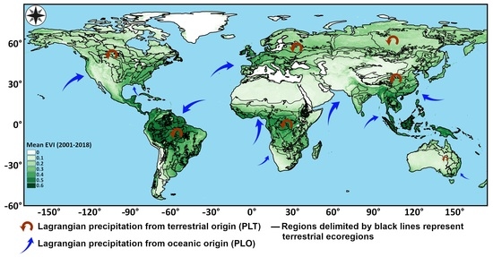
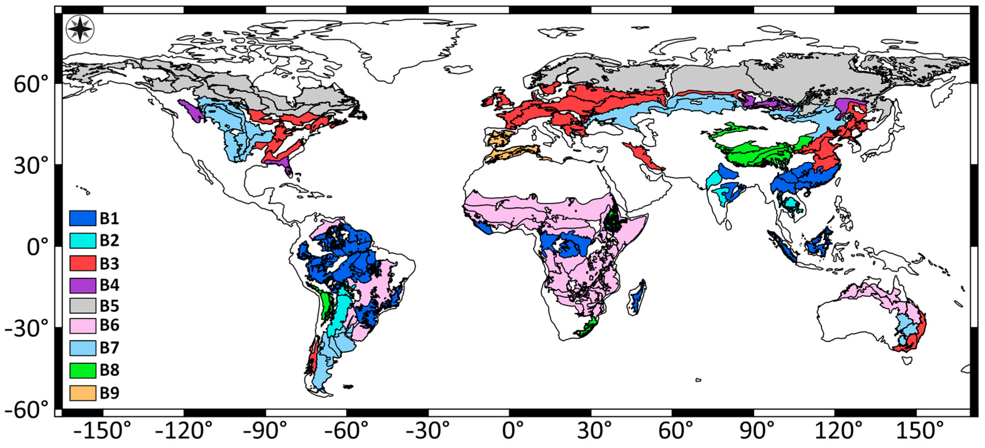
2.1. Study Regions

This study was conducted for 9 terrestrial biomes, which are the main global plant communities based on homogeneous rainfall and climate characteristics, and they were also divided into 139 ecoregions. The main biomes of the world are distinguished by specific climatic conditions (e.g., precipitation and temperature). Forests are one of the most significant groups of terrestrial biomes, covering around one-third of the continental area of the Earth [68]. Additionally, ecoregions are part of biomes, representing areas that are geographically and ecologically similar, and experience similar climatic conditions [69]. Arid, semiarid, and desert areas are characterized by low precipitation rates and available water for vegetation, which inhibit most plants from surviving, and thus, the productivity is negligible. For this reason, these areas were not considered in this study. Figure 1 illustrates the 9 terrestrial biomes and 139 ecoregions with areas greater than 200,000 km² for each major habitat type (biome) used in this study. The nine biomes are tropical and subtropical moist broadleaf forests (with 30 ecoregions); tropical and subtropical dry broadleaf forests (5); temperate broadleaf and mixed forests (24); temperate coniferous forests (4); boreal forest/taiga (17); tropical and subtropical grasslands, savannas, and shrublands (27); temperate grasslands, savannas, and shrublands (19); montane grasslands and shrublands (10); and Mediterranean forest woodlands and scrub (3). The major forest biomes worldwide are tropical, temperate, and boreal forests (tundra) [70]. Tropical and subtropical moist forests are characterized by high variability in precipitation (>2000 mm/year) and low variability in temperature [69]. Thus, their structure is characterized by semi-evergreen and evergreen deciduous tree species. These forests are usually located in equatorial regions, in the Indo-Malayan Archipelagos, the Amazon Basin in South America, and the African Congo. A constantly warm, humid climate leads to increased plant growth compared with other biomes [69]. In contrast, low annual temperatures with precipitation ranging between 400 and 1000 mm/year and low evaporation due to cold temperatures prevail in the boreal forest (taiga). This biome is the world’s largest terrestrial biome and is found across Canada, Alaska, Russia, and northern Europe. The long, cold winters in boreal forests have led to the predominance of cold-tolerant, cone-bearing plants, such as pines, spruces, and firs. For each ecoregion, we used boundaries identified by the World Wildlife Fund (WWF) in The Global 200: Priority Ecoregions for Global Conservation [71].

2.2. Data

The spatial extension of the biomes and ecoregions was obtained from the WWF with a horizontal resolution of 0.25°. Ecoregions with areas greater than 200,000 km² were selected, resulting in 139 terrestrial ecoregions.

The global precipitation and temperature dataset from the Climate Research Unit (CRU) TS v4.05 at 0.5° (P_CRU) [72] was utilized to obtain the precipitation series over each biome and the associated ecoregion. These data are generated by the interpolation of monthly climate anomalies from widespread networks of weather station observations, which guarantees a realistic representation of precipitation, particularly over densely monitored regions. As precipitation amounts can change from month to month in many parts of the world and not all databases represent them completely reliably, global datasets of precipitation from ERA-Interim reanalysis (P_ERA) [73] were also used. Both the datasets were interpolated to 0.25° resolution. For this purpose, the ordinary kriging interpolation method was used, as it has demonstrated accurate estimates of plant diversity values [74,75]. Global monthly radiation datasets with this resolution were also downloaded from the ERA5 reanalysis project [76]. The study was performed for the 2001–2018 period.

Global monthly gridded datasets of Lagrangian precipitation from oceanic (PLO) and terrestrial (PLT) origins with a spatial resolution of 0.25° obtained by Nieto and Gimeno (2019, 2021) [77,78] were used. For this calculation, the authors used the FLEXible PARTicle dispersion model (FLEXPART) [79,80], which uses ERA-Interim reanalysis datasets. This approach considers the atmosphere divided into 61 vertical levels and approximately 2 million particles that are tracked forward in time using the 3D winds and specific humidity. Along the trajectories and in 6 h time (t) intervals, the specific humidity (q) changes in each particle were computed by computing the gain (through evaporation from the environment, e) or loss (through precipitation, p), using Equation (1).

$$\left(e-p\right)=m\left(\frac{dq}{dt}\right)$$

(1)

Integrating this budget in the vertical column permits us to obtain the budget of the total evaporation (E) minus precipitation (P), which represents the freshwater flux (E − P). Negative values of (E − P) are therefore an approximation of precipitation. Thus, the values of PLO (PLT) over continental regions were obtained in the experiment forward in time by obtaining the (E − P) < 0 over the terrestrial areas on air masses tracked forward in time from entirely oceanic (terrestrial) regions. The sum of PLO and PLT results in the total Lagrangian precipitation, which is an approximation of the ERA Interim precipitation. The optimal integration times (in days) for each grid were taken into account in order to achieve the best approximation of precipitation according to three databases. The approach used by several researchers through this modelling experiment has proven to be a reliable tool for investigating the atmospheric branch of the hydrological cycle. These datasets have also been recently used to investigate the precipitation trend over continents [40] and to assess the frequency and severity of drought episodes over major world river basins [54].

In this study, we utilized monthly EVI values for the period 2001–2018. These cover 18 years and consequently consist of 216 values. Using the complete continuous series guarantees the introduction of the temporal (seasonal, inter-annual) variations of the greenness stages. The EVI time series was extracted from the moderate resolution imaging spectroradiometer MODIS/Terra Vegetation Indices (MOD13C2) at 0.05° obtained from the Land Processes Distributed Active Archive Center (LP DAAC) and the U.S. Geological Survey (USGS) Earth Resources Observation and Science (EROS) Center [81] at https://lpdaac.usgs.gov (accessed on 31 October 2021). Remotely sensed vegetation indices from satellite data have been widely used to characterize vegetation dynamics at regional and global scales [82,83]. We chose this index because, compared to other datasets, it is based on narrow-band calculations specifically designed for vegetation monitoring and is a quality-controlled global-gridded dataset which benefits from upgraded radiometric feeling and atmospheric conditions [84]. The EVI index has been modified for some atmospheric conditions and canopy background noise and is more sensitive than the NDVI in high-biomass areas [85,86]. It incorporates an “L” value which represents a canopy background adjustment, “C” values as coefficients for atmospheric resistance, G as a gain or scaling factor, and values from the blue band (blue). These improvements make it possible in most cases to calculate the index with a reduction in background noise, atmospheric noise, and saturation. The index ranges in value between −1 (surface water) and +1 (complete, lively canopy). According to Chen et al. (2006) [87] and Ayanlade (2017) [88], healthy vegetation with high chlorophyll content (e.g., forests) will produce high EVI values near 1, while poor (drier) vegetation will produce values below 0.5 (indicating sparse canopies). The EVI dataset used here is derived from atmospherically corrected reflectance in the red, near-infrared, and blue wavebands. Due to its rationing properties, a large proportion of signal variations attributed to calibration, noise, and changing irradiance conditions is removed, permitting us to obtain the Vegetation Index (VI) time series directly. In our analysis, EVI values greater than 0.1 were utilized, ensuring that everything from shrub and grassland areas to temperate and tropical rainforests and crops areas at their peak growth stage were considered. The higher the value, the denser the vegetation. We removed negative values associated with water and snow surfaces, and clouds, as well as values close to zero (0.1 and below), which correspond to areas of rock and sand [81]. This avoids the inclusion of sensitivity values with no real ecological significance.

The choice of EVI as the only index for this study took into account its advantages over other indices, its temporal availability, and its ability to represent vegetative activity in different types of climates and ecosystems. An assessment of the MODIS vegetation indices showed that NDVI values present a greater range over the semiarid regions, but at the expense of a lower dynamic range over the more humid forested sites, where the EVI remained sensitive to canopy variations [84]. Additionally, these authors also found a good correspondence between airborne-measured, top-of-canopy reflectances and VI values and those from the MODIS sensor at four intensively measured test sites representing semi-arid grass/shrub, savanna, and tropical forest biomes. Another study confirmed a good relationship between EVI and Leaf Area Index (LAI) in five sites around the world characterized by different vegetation types in dry and warm tropical climatic conditions [89]. Additionally, regional studies (e.g., Northwest China) have also confirmed the ability of the EVI to characterize different vegetation types (e.g., broadleaf forests, needle leaf forests, meadows, grassland, steppes, scrubs, desert, and cultivated vegetation) and even represent crop growth better than NDVI [90]. Despite the good performance of the EVI in representing vegetative activity, there are indices such as the MCTI that have outperformed it. However, the period of data available for the MCTI was shorter than that available for the EVI. An assessment of the radiometric and biophysical performance of the MODIS vegetation indices showed that NDVI values present a greater range over the semiarid regions, but at the expense of a lower dynamic range over the more humid forested sites, where the EVI remained sensitive to canopy variations [82]. Additionally, these authors also found a good correspondence between airborne-measured, top-of-canopy reflectances and VI values and those from the MODIS sensor at four intensively measured test sites representing semi-arid grass/shrub, savanna, and tropical forest biomes. Another study confirmed a good relationship between EVI and Leaf Area Index (LAI) in five sites around the world characterized by different vegetation types in dry and warm tropical climatic conditions [89]. Additionally, regional studies (e.g., Northwest China) have also confirmed the ability of the EVI to characterize different vegetation types (e.g., broadleaf forests, needle leaf forests, meadows, grassland, steppes, scrubs, desert and cultivated vegetation) and even represent crop growth better than NDVI [90].

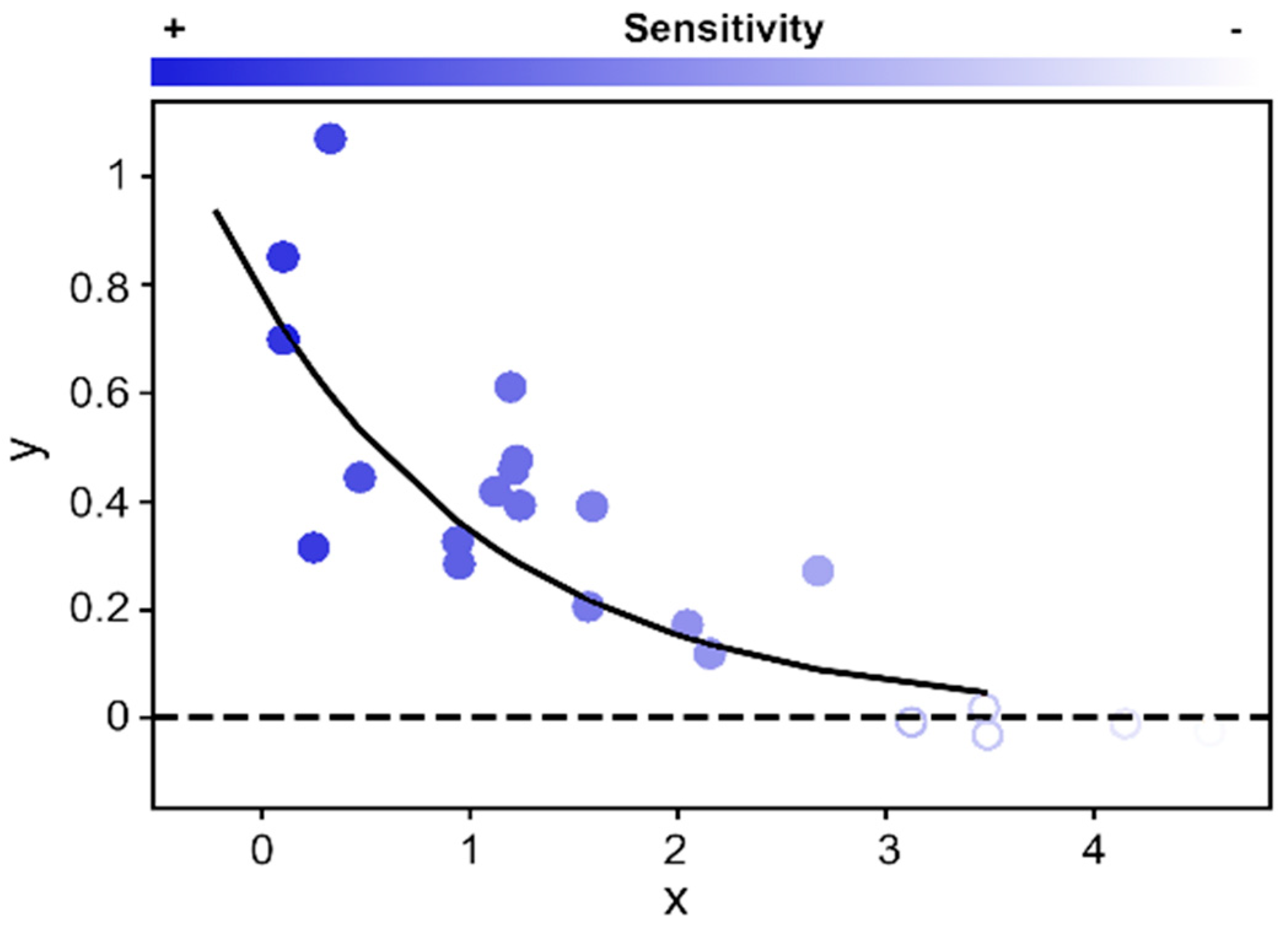
2.3. Vegetation Greenness Sensitivity (VGS) Metric and Statistical Analyses

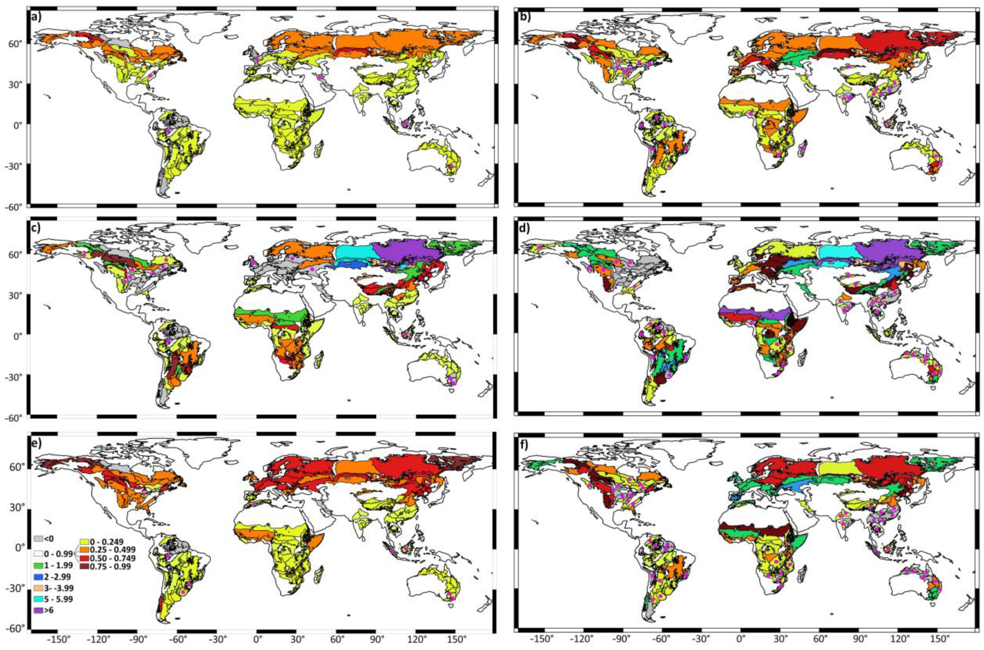
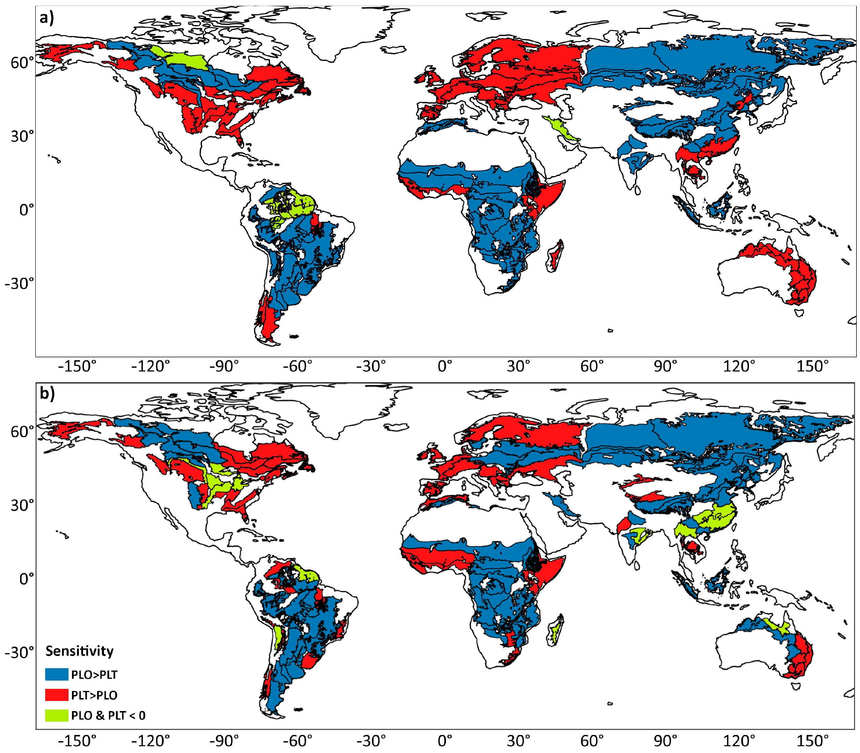
We performed a sensitivity analysis to understand vegetation changes in each biome and ecoregion due to precipitation of oceanic and terrestrial origins. In the first step, a linear regression was used to estimate the mean temporal relationship between primary production (EVI), which is the dependent variable (y), and the independent variables (x), which are P_CRU, PLO, and PLT, as represented by Equation (2).

$$y=ax+b$$

(2)

The same approach has been used in previous investigations (e.g., [91,92]). In regions where the sensitivity of vegetation to variables other than precipitation is higher, our results would be attenuated by the effect of these variables. Thus, the VGS was also calculated after removing the compound effects of two crucial variables on the vegetative activity, the temperature and radiation. This was achieved by means of multiple regression analysis, following a residualization technique. The first step is to fit a regression model with EVI (y) as dependent, and the temperature (t) and radiation (r) as independent variables (Equation (3)). Afterward, the residuals (Yr) are calculated, which represent the remaining variation in ‘y’ after accounting for the effects of temperature and radiation, and they are used to perform individually the following regression with P_CRU, PLO, and PLT (Equation (4)).

$$y=at+br+u$$

(3)

$$Yr=ax+b$$

(4)

To confirm the statistical significance, we used a p-value at the 95% confidence level. Finally, the sensitivity values are fitted to an exponential model to adjust individual sensitivities for changes in P_CRU, PLO, and PLT and observe the VGS distribution among ecoregions of the same and different biomes. The VGS units were expressed as the change in monthly EVI per unit (mm/year) of change in P_CRU, PLO, and PLT. Figure 2 illustrates an example, where y characterizes the VGS and x characterizes the independent variable. The figure shows that the VGS fluctuates over the range of x (P_CRU, PLO, and PLT). When x is lower, a minor alteration in x corresponds to a great alteration in VGS, meaning a higher sensitivity. The sensitivity is minor when x is greater because a great change in x produces a minor alteration in y.

3. Results

The VGS to variations of P_CRU, PLO, and PLT by biome and ecoregion, after also removing the effects of temperature and radiation, is shown in Figure 3. The sensitivity was determined using monthly values. The analysis indicated that the major VGS to P_CRU occurs in the temperate broadleaf and mixed forest (B3); boreal forest/taiga (B5); and temperate grasslands, savannas, and shrublands (B7). However, greater values of sensitivity were observed when the effects of temperature and radiation were removed (Figure 3a,b). In contrast, the vegetation sensitivity of tropical and subtropical moist broadleaf forest ecoregions (B1) to P_CRU is lower. In the rest of the biomes and ecoregions, the vegetation response to the P_CRU was mostly positive. When the effects of temperature and radiation are removed (Figure 3b), the VGS to P_CRU, PLO, and PLT shows a similar fitting pattern, but the values seem to be higher, although the number of non-statistically significant (p < 0.05) values increased.

The spatial representation of VGS shown in Figure 3, according to the EVI to P_CRU, PLO, and PLT without removing and after removing the compounding effects of temperature and radiation, appears in Figure 4a–f. These values were determined according to the temporal variations of greenness and precipitation for individual eco-zones. For P_CRU, as illustrated in Figure 4a, the response of vegetation productivity was highly similar in ecoregions of South America, Africa, southeast Asia, and Australia. This pattern is highlighted, however, because of the major VGS exhibited in boreal high-latitude ecoregions across Europe, Asia, and North America, where precipitation is lower than in humid tropical regions. In this figure, it can be observed that a few ecoregions experience a negative VGS which is not statistically significant. These include the southern tip of South America occupying B7, northern Western Europe (B3), and some regions of B1 in the extreme southwest region of Amazonia. When the joint effect of temperature and radiation is removed (Figure 4b), the VGS values become more heterogeneous among the biome ecoregions, with those of biomes 2 and 6, located south of the Amazon, standing out, as well as those ecoregions located in the Sahel and Equatorial Africa (B1, B6). This figure also confirms the higher VGS in the ecoregions of northern Eurasia, with the ecoregions of biomes 7 and 9 in the Iberian Peninsula, Central Europe (B3), and northeastern Eurasia (B5) standing out. Additionally, ecoregions with negative sensitivity are observed in Southeast Asia, particularly in China.

The VGS to PLO (Figure 4c) revealed a pronounced change between the maximum and minimum values among all the biomes and ecoregions, showing the highest values in the boreal forest/taiga ecoregions of biome 5, in the north of North America and the north and northeast of Eurasia. Negative values indicating non-sensitivity were obtained for various ecoregions of B1 in the Amazonia, and ecoregions in B3 that occupy a large part of central and western Europe, excluding the Mediterranean forest woodlands and scrub (B9) that occupy the Iberian Peninsula. Not statistically significant sensitivity values are mostly observed in various ecoregions of B1 in the Amazon basin, but also in the northeast of North America and central Europe. Figure 4d reveals that after removing the compounding effects of temperature and radiation, the magnitude of VGS values varies from those observed in Figure 4c. Most notably, VGS values in Western Europe are now positive. The contrary occurs in ecoregions located in Southeast Asia, East China, and the northeast of North America. A large number of ecoregions with not statistically significant (p < 0.05) VGS values are also observed.

A longitudinal gradient of VGS is best observed in the ecoregions of B5 along northern Eurasia (Figure 4c,d). These figures also illustrate marked similarities and dissimilarities in the spatial response of vegetation activity to PLT when the compound effect of both temperature and radiation was removed. Figure 4e shows a few differences in VGS among the ecoregions, highlighting the major differences in North America and Eurasia. Our findings also highlight the European ecoregions where, contrary to the role of PLO, the vegetation is more sensitive to PLT. When the effect of temperature and radiation is removed, the VGS to PLT reveals noticeable changes (Figure 4f) with respect to the values depicted in Figure 4e. The most evident is that VGS becomes negative and mostly non-statistically significant in East and Southeast Asia (B1, B2). Additionally, Figure S2 shows the VGS to PLO and PLT, also considering the removed effects of temperature and radiation.

The total number of ecoregions by biomes, with positive and negative VGS values without removing and after removing the compound effects of temperature and radiation, expressed as a percentage, is shown in Table S1. Likewise, in this table, the area occupied by the respective ecoregions is also shown in percentage. This information summarizes numerically what can be observed in Figure 4. A greater number of ecoregions that belong to B1 experience a positive VGS to P_CRU, PLO, and PLT. However, the area they occupy is very similar to the total area occupied by ecoregions with negative VGS, confirming the importance of the spatial extension of the ecoregions. This disproportionality is also observed for other biomes, such as B2, which stand out because the vegetation of all ecoregions experiences a positive sensitivity to P_CRU, PLO, and PLT. To summarize, the frequency distributions of the VGS illustrated in Figure 4c–f are represented by histograms in Figure 5. For the VGS to EVI (Figure 5a), the number of ecoregions with negative sensitivity values is higher for PLO than PLT. Additionally, there is a larger number of ecoregions with a positive response to PLT (128 ecoregions) than to PLO (110), although the highest levels of sensitivity (>1) are due to changes in PLO. Ecoregions with negative sensitivity sum up to 27 for PLO and 24 for PLT. Similar results were found for the sensitivity assessed after removing the effect of temperature and radiation (Figure 5b). In this case, we confirmed that a large number of ecoregions (117) also experienced higher positive VGS to PLT, while only 112 did for PLO. In both graphs, the positive values, which indicate the degree of sensitivity, range between 0 and 1, with a greater frequency observed to PLT. However, according to Figure 5b, the VGS values greater than 1 were also more frequent, owing to the PLO. Table S2 shows the percentage of the number of ecoregions with non-significant sensitivity by each of the histogram ranges, confirming the small number of cases for the positive values.

Figure 6a summarizes the major role of precipitation from oceanic and terrestrial origin in the VGS according to EVI. Figure 6b also shows the same metric but considers the VGS obtained after removing the compound effects of the temperature and radiation. Ecoregions that are most sensitive to PLT are shaded in red, to PLO in blue, and those with negative sensitivity for both are shaded in light green. In the first analysis, 60% of the ecoregions considered for this study showed greater VGS to PLO, followed by 34% to PLT, and only in 6% did both variables have no direct effect. In a more realistic analysis, after removing the influence of temperature and radiation on the variability of vegetative activity (Figure 6b), a very similar spatial pattern is observed, with 58% of ecoregions showing vegetation that is more sensitive to changes in PLO, 32% to PLT, and in 10%, the sensitivity values are negative, and therefore do not contribute to the understanding of changes in greenness.

The predominant sign of VGS in North America represented in Figure 6a demonstrates some variation among ecoregions when the influence of temperature and radiation is removed, as illlustrated in Figure 6b. In this figure, some ecoregions stand out, such as those located in the central east and belonging to biomes 2 and 3, mainly due to the negative sign (Figure 6b). Of the remaining ecoregions, only those in the northwest that belong to B5, and one in the central United States (B2), are more sensitive to changes in PLO. In South America, the vegetation greenness in most of the ecoregions experiences a major sensitivity to changes in precipitation of oceanic origin. Furthermore, in areas of the central and northeastern Amazon region, the negative values of vegetation productivity to both PLO and PLT confirm that vegetation is not constrained by water availability. In this region, other factors like cloudiness and temperature play a major role [93].

In Southeast Asia, some ecoregions of tropical and subtropical moist and dry broadleaf forests (B1 and B2) experience greater sensitivity to PLT (Figure 6a). However, the effects of radiation and warming on greening in these regions have been documented [94], and consequently, removing their effects resulted in negative VGS values. Similarly, this also occurs in the northern and eastern ecoregions of Australia (Figure 6a), which belong to (1) the biomes of temperate broadleaf and mixed forest (B3); (2) tropical and subtropical grasslands, savannas, and shrublands (B6); and (3) temperate grasslands, savannas, and shrublands (B7). Our results show that precipitation can play a distinct role in the dynamics of vegetation if its components are analyzed independently, which is a useful approach for understanding the role of global warming in precipitation variability and its impact on vegetation. The question arises as to what will happen in different global warming scenarios, in which the influence of the precipitation components may vary with respect to what is observed or reinforce the conditions described above.

4. Discussion

The climatological distribution of radiation, temperature, and precipitation on the planet is a key factor determining the behavior of vegetative activity. Accordingly, the values of VGS to P_CRU show remarkable differences, mainly latitudinal, between biomes and even between biome ecoregions themselves. The lower values of VGS to precipitation obtained for the vegetation of humid equatorial ecoregions (Figure 4a,b) are in agreement with previous studies. Zhang et al. (2022) [51] found that the mean sensitivity of vegetation canopy greenness to precipitation is highest in drier and arid regions and decreases in more humid regions. In drier regions, vegetation constraints on plant growth responses to precipitation are hypothesized to place an upper limit on net primary productivity [95]. However, Hilker et al. (2014) [96] found that the vegetation canopy of the Amazon rainforest is highly sensitive to changes in precipitation, revealing that the Amazon forest greens during the dry season because of the light limitations during the wet season and insufficient water supply for deep-rooted trees. Our results also confirm that in the vast majority of ecoregions, there is an increase in VGS to precipitation after removing the influence of temperature and radiation, including the vegetation of humid tropical regions such as the Congo and the Sahel. Other factors already documented are forest height and age, which are important in the control of photosynthesis in response to interannual precipitation fluctuations [97].

The terrestrial origin moisture, transported across the continents, and local recycling increase the terrestrial origin precipitation in high-latitude boreal ecoregions [40,54]. In these regions, the observed greater VGS to P_CRU, which is even greater when not considering the effect of temperature and radiation (Figure 4a,b), must be associated with the temperature shift, bearing in mind that at high latitudes in the Northern Hemisphere, vegetation is more sensitive to changes in temperature than to changes in precipitation [98]. However, these authors also found that around 18.48% of the world is more sensitive to precipitation than to temperature. In boreal high latitudes, the effect of temperature is also higher than that of precipitation, making these regions energy-limited areas [99]. This phenomenon is particularly observed in northern Western Europe ecoregions, and also in some wetter terrestrial ecoregions, as commented above, located in the Amazonia that belong to B1, where energy supply, not water supply, limits evapotranspiration. In these ecoregions, the negative sensitivity of vegetation greenness to precipitation indicates that precipitation is not the primary variable controlling vegetation productivity because of the primary role of radiation and air temperature [100]; however, it could play a secondary role. Alternatively, in drier zones characterized by water-limited conditions, precipitation generally becomes the main impacting factor, as freshwater resources are limited, which results in a restrictive condition for the vegetation [10,100]. A study by Seddon et al. (2016) [101] also showed that prairies in mid-northern hemisphere latitudes are water-limited, high latitudes are driven by a combination of temperature and cloudiness, and tropical forests are particularly sensitive to cloudiness.

As commented above, our results are in agreement with previous studies, which documented that vegetation in humid ecoregions is more sensitive to changes in solar radiation followed by temperature and precipitation [102]. In those regions characterized by high annual precipitation rates, the rainfall becomes a less limiting factor on vegetation growth, which is, in contrast, modulated by the effects of temperature and radiation [21]. In this way, the VGS values depicted in Figure 4b objectively represent more realistically the vegetative response to changes in precipitation. However, to obtain more accurate results, the influence of other factors should have been taken into account. For instance, other studies have determined that additional water resources like groundwater will also reduce the direct dependency of vegetation on precipitation [103], as well as other local constraints on plant growth, like nutrients [104].

Precipitation contributes to soil moisture and part of it is retained by vegetation. However, this precipitation has a percentage of oceanic and terrestrial origin, and it is variable on our planet. There are regions, like those near the coasts of the continents, characterized by a major percentage of precipitation of oceanic origin, while in inland regions, the percentage of precipitation of terrestrial origin exceeds that of oceanic origin [40]. The VGS calculated considering the terrestrial and oceanic components of precipitation is an analysis that has not been performed before, and it takes into account the dynamics of the atmospheric branch of the hydrological cycle and terrestrial and oceanic evaporation processes to explain the vegetative response. Our analysis shows precisely that, in some ecoregions located in eastern North America, northern Amazonia, and western Europe, except the Iberian Peninsula, where the major percentage of precipitation is due to PLO [40], the VGS values obtained are negative (Figure 4c). The historical changes in zonal vegetation patterns across the Iberian Peninsula have been utilized to investigate annual precipitation variability and trends and their local patterns over 11 700 years [105]. After removing the joint effect of temperature and radiation, the resulting values of VGS to PLO (Figure 4d) reveal that Western European ecoregions now exhibit positive values. In this region of the planet, the VGS is mainly modulated by temperature [98], so this result confirms that the major precipitation component over this region influences vegetation activity, but in agreement with other studies, it also draws attention to possible uncertainties of different methodologies in representing the complex interactions between climate and vegetation [98]. For Southeast Asia, in contrast, the VGS cannot be explained after removing the role of temperature and radiation, in agreement with findings obtained with P_CRU (Figure 4b).

In other ecoregions characterized by energy-limited conditions (where P/Etp > 1), such as northern Eurasia, part of the Amazon, and Central Equatorial Africa [94], the energy supply and not the water supply limits the actual evapotranspiration (i.e., the amount of water that is removed from the surface due to the processes of evaporation and transpiration). In these regions, PLT is greater than PLO [40], owing to intense recycling and moisture exports within the continent [43]. In our analysis (and previous studies), we found that in regions with high rainfall regimes (humid regions), the sensitivity of vegetation to rainfall is lower because precipitation is not a limiting factor, and the opposite was found in regions with a low rainfall regime. Therefore, we should expect that VGS is greater (lower) to the minor (major) component of precipitation. Hence, vegetation is more sensitive to changes in PLO in those ecoregions where precipitation is mostly from terrestrial origin. The opposite is observed in a large part of Western Europe, parts of central eastern North America, and the southeast of the United States, which belong to B3 and B4, respectively. The predominance of precipitation of oceanic origin in these regions [40] makes the vegetation more sensitive to changes in PLT, as shown in Figure 4e,f. In Africa, two differentiated regions are situated on the coast of West Africa and Ethiopia, where the VGS to PLT without eliminating and after eliminating the joint effect of temperature and radiation is higher than in the rest of the ecoregions of that continent. In both regions, the oceanic contribution to precipitation is higher and directly modulated by the moisture supply from the Gulf of Guinea [106,107] and the western Indian Ocean [108,109], respectively. Vegetation in both regions is therefore more sensitive to slight changes in precipitation of terrestrial origin. In the Sahel zone, the VGS is lower than that exhibited with PLO, because of the crucial role of the predominant evapotranspiration and recycling process in maintaining and determining the annual cumulative precipitation in this region [110]. Previous studies have found that the NDVI response to precipitation in the Sahel occurs at seasonal scales, although inter-annual fluctuations in precipitation also coincide with fluctuations in the NDVI values [49], which suggests that further research on this topic, while considering lag times, should be carried out.

As explained above, by separating the effects of the precipitation components, we are likely to spatially delineate ecoregions where vegetation is most sensitive to changes in precipitation due to the major variability of one of its components. This differentiation is well observed in Eurasia, where the west is more sensitive to changes in PLT (Figure 4c–f) due to the more stable character of the oceanic precipitation generated by moisture transport from the Atlantic and the Mediterranean [111,112]. However, in central north and northeast Eurasia, PLT is predominant [40], and the variability of PLO originating from moisture fluxes from oceanic regions makes vegetation more susceptible. Other studies (e.g., Seddon et al. (2016) [101]) found that central and western continental Europe demonstrates a stronger water limitation in comparison with temperature and radiation, while other authors [97] have also described the east–west vegetation sensitivity gradient to precipitation and temperature. This is probably why removing the joint effect of temperature and radiation generally increases the VGS in this region. However, in several ecoregions of Southeast Asia and eastern China, it is observed that after removing the compound effects of temperature and radiation, negative VGS values to PLO and PLT (Figure 4d,f) are demonstrated, which represents a more realistic dynamic, as obtained in the sensitivity analysis of P_CRU (Figure 4b).

Other results show that precipitation in the half-east of North America is mainly modulated by precipitation originating from oceanic origin [94], and consequently, vegetation is more sensitive to alterations in the terrestrial component (Figure 4c–f), while the contrary is observed for the northwest ecoregions. Something similar occurs in Africa, where the sensitivity to PLT is higher in those regions where moisture transport mechanisms increase the oceanic origin precipitation (the southern coast of West Africa and the Ethiopian area). Precipitation from an oceanic tropical origin is normally dominant in these regions [113]. Furthermore, this pattern is also seen in Australia, where the crucial role of humidity transport from the surrounding Pacific and Indian Oceans has been well-documented [114]. The subsequent analysis also revealed that this homogeneity changes, with ecoregions with a predominance of VGS to PLO, to PLT, and even negative joint values. Previous findings have also described that the warming of some biomes in northern ecosystems affects greening, while precipitation anomalies in tropical biomes caused browning associated with climate change [115].

Precipitation plays a decisive role in vegetative development by supplying the water necessary for plant germination and growth. However, the amount of precipitation over a region depends on the moisture that is transported from oceanic and/or terrestrial regions. Therefore, in studies on the attribution of causes of changes in vegetation sensitivity due to changes in precipitation, the amount of the oceanic and terrestrial Lagrangian components of precipitation should be taken into account. There are regions, such as the Congo Basin, for example, where the major percentage of precipitation is produced by recycled precipitation and evapotranspiration [46,116], but findings of Gimeno et al. [40] confirmed the growing importance of precipitation from oceanic origin over tropical regions, which could modulate the vegetation sensitivity along the influencing areas. The consideration of both components also represents an opportunity to understand the role of global warming in the atmospheric branch of the hydrological cycle, the precipitation variability, and the vegetation response. This also applies to future studies considering the observed and expected changes in the hydrological cycle [117,118]. It should also be mentioned that although the Lagrangian methodology has been widely used for the study of the hydrological cycle, it also has limitations, as it does not specifically represent precipitation, which affects the comparative analyses that can be carried out with precipitation data. Similarly, the estimated values of (E − P) < 0 will be better correlated with the model input precipitation data (ERA-Interim precipitation). In this study, we use a different database to avoid any possible collinearity. The effectiveness of our results also depends on the methodology used. Multiple studies have used the same regression analysis; however, others have opted to use polynomial regression [97] or land surface models [119] to represent non-linear relationships, which represent an advantage principally for studies at local and regional scales.

5. Conclusions

This study aimed to investigate the global vegetation greenness sensitivity (VGS) to precipitation over the period of 2001–2018, and separately considered precipitation from oceanic and terrestrial origins. We quantified the VGS in 9 biomes consisting of 139 ecoregions worldwide for the period of 2001–2018 through the satellite vegetative index EVI, precipitation, and oceanic and terrestrial Lagrangian precipitation data. Without taking into account arid and semi-arid regions, and by removing the compound effects of temperature and radiation, our results are in accordance with previous findings, confirming that moist broadleaf forest and wetland vegetation in Amazonia, Oceania, and southeast Asia generally experience smaller and even negative VGS to precipitation than other vegetation types. This was also observed in a few other ecoregions characterized by temperate broadleaf and mixed forests (B3) and temperate grasslands, savannas, and shrublands (B7) and temperate broadleaf and mixed forests in northwest Europe. In the rest of the ecoregions, a positive relationship was found. According to the literature, the greatest VGS to precipitation occurs in tropical and subtropical arid, semiarid, and desert regions located in areas of North Africa, the Arabian Peninsula, South Africa, Australia, and central South America, but these regions were not taken into account in this study. Consequently, our analysis confirmed that vegetation greenness is more sensitive to precipitation changes in high-latitude ecoregions of the Northern Hemisphere. We confirmed the veracity of these results after removing the compound effects of temperature and radiation, which play a key role in vegetation productivity. The VGS in each ecoregion according to the EVI was also studied, but considering the oceanic and terrestrial components of the precipitation individually. These results revealed notable differences in the VGS magnitude between ecoregions of the same biome that were geographically distant. This was mostly observed among the ecoregions of Biome 5 (boreal forest/taiga), located in North America, Europe, and North Asia, but particularly in the European temperate broadleaf and mixed forests. Additionally, and in agreement with what was obtained for precipitation, neither PLO nor PLT controlled vegetation greenness in some ecoregions of central and northeast Amazonia, where climatological high precipitation makes the vegetation productivity more susceptible to other factors. Removing the joint effect of temperature and radiation resulted in changes in VGS values, allowing a more realistic characterization of vegetation dynamics. Finally, we found that normally, the greenness sensitivity is more affected by fluctuations in PLT (PLO) in climatological regions with a major rate of PLO (PLT). As the contribution to precipitation by the dominant component of the precipitation is more stable, the variations in the contribution of the minor component can affect the average water availability, and consequently the vegetation greenness. Thus, in regions with high rainfall regimes (humid regions), the sensitivity of vegetation to rainfall is lower due to its small variation during the year, and the opposite occurs in regions with a low rainfall regime. These results reveal the importance of considering the intrinsic climate variability on the assessment of precipitation variability resulting from global oceanic evaporation and terrestrial evapotranspiration and their contribution to water availability and vegetation greenness. However, an assessment of the VGS, simultaneously considering other climatic and anthropogenic factors across the global land, is lacking. It represents a challenge and support for investigating the ecosystem’s development and its functionalities in the present and future climate and vegetation scenarios. Ongoing simulation of future moisture transport will support the studies of vegetation response to hydroclimatic changes.

References

1. Han, F.; Yan, J.; Ling, H.B. Variance of vegetation coverage and its sensitivity to climatic factors in the Irtysh River basin. PeerJ 2021, 9, e11334. [Google Scholar] [CrossRef]
2. Li, M.; Song, Y.; Huang, X.; Li, J.; Mao, Y.; Zhu, T.; Cai, X.; Liu, B. Improving mesoscale modeling using satellite-derived land surface parameters in the Pearl River Delta region, China. J. Geophys. Res. Atmos. 2014, 119, 6325–6346. [Google Scholar] [CrossRef]
3. Zhang, W.; Luo, G.; Chen, C.; Ochege, F.U.; Hellwich, O.; Zheng, H.; Hamdi, R.; Wu, S. Quantifying the Contribution of Climate Change and Human Activities to Biophysical Parameters in an Arid Region. Ecol. Indic. 2021, 129, 107996. [Google Scholar] [CrossRef]
4. Wang, W.L.; Anderson, B.T.; Phillips, N.; Kaufmann, R.K.; Potter, C.; Myneni, R.B. Feedbacks of vegetation on summertime climate variability over the North American grasslands. Part I: Statistical analysis. Earth Interact. 2006, 10, 1–5. [Google Scholar] [CrossRef]
5. Fay, P.A.; Kaufman, D.M.; Nippert, J.B.; Carlisle, J.D.; Harper, C.W. Changes in grassland ecosystem function due to extreme rainfall events: Implications for responses to climate change. Glob. Chang. Biol. 2008, 14, 1600–1608. [Google Scholar] [CrossRef]
6. Kong, D.; Zhang, Q.; Singh, V.P.; Shi, P. Seasonal vegetation response to climate change in the Northern Hemi-sphere (1982–2013). Glob. Planet. Chang. 2017, 148, 1–8. [Google Scholar] [CrossRef]
7. Weltzin, J.F.; Loik, M.E.; Schwinning, S.; Williams, D.G.; Fay, P.A.; Haddad, B.M.; Harte, J.; Huxman, T.E.; Knapp, A.K.; Lin, G.; et al. Assessing the response of terrestrial ecosystems to potential changes in precipitation. Bioscience 2003, 53, 941–952. [Google Scholar] [CrossRef]
8. Zhao, F.; Wu, Y.; Sivakumar, B.; Long, A.; Qiu, L.; Chen, J.; Wang, L.; Liu, S.; Hu, H. Climatic and Hydrologic Controls on Net Primary Production in a Semiarid Loess Watershed. J. Hydrol. 2019, 568, 803–815. [Google Scholar] [CrossRef]
9. Piao, S.; Mohammat, A.; Fang, J.; Cai, Q.; Feng, J. NDVI-based increase in growth of temperate grasslands and its responses to climate changes in China. Glob. Environ. Chang. 2006, 16, 340–348. [Google Scholar] [CrossRef]
10. Wang, J.; Wang, K.; Zhang, M.; Zhang, C. Impacts of climate change and human activities on vegetation cover in hilly southern China. Ecol. Eng. 2015, 81, 451–461. [Google Scholar] [CrossRef]
11. Zheng, K.; Wei, J.; Pei, J.; Cheng, H.; Zhang, X.; Huang, F.; Li, F.; Ye, J. Impacts of climate change and human activities on grassland vegetation variation in the Chinese Loess Plateau. Sci. Total Environ. 2019, 660, 236–244. [Google Scholar] [CrossRef]
12. Papagiannopoulou, C.; Miralles, D.G.; Dorigo, W.A.; Verhoest, N.E.C.; Depoorter, M.; Waegeman, W. Vegetation anomalies caused by antecedent precipitation in most of the world. Environ. Res. Lett. 2017, 12, 074016. [Google Scholar] [CrossRef]
13. Maurer, G.E.; Hallmark, A.J.; Brown, R.F.; Sala, O.E.; Collins, S.L. Sensitivity of primary production to precipitation across the United States. Ecol. Lett. 2020, 23, 527–536. [Google Scholar] [CrossRef] [PubMed]
14. Ayanlade, A.; Jeje, O.D.; Nwaezeigwe, J.O.; Orimoogunje, O.O.I.; Olokeogun, O.S. Rainfall seasonality effects on vegetation greenness in different ecological zones. Environ. Chall. 2021, 4, 100144. [Google Scholar] [CrossRef]
15. Soomro, S.; Hu, C.; Jian, S.; Wu, Q.; Boota, M.W.; Soomro, M.H.A.A. Precipitation changes and their relationships with vegetation responses during 1982–2015 in Kunhar River basin, Pakistan. Water Supply 2021, 21, 3657–3671. [Google Scholar] [CrossRef]
16. Wang, J.; Rich, P.M.; Price, K.P. Temporal responses of NDVI to precipitation and temperature in the central Great Plains, USA. Int. J. Remote Sens. 2003, 24, 2345–2364. [Google Scholar] [CrossRef]
17. Hawinkel, P.; Thiery, W.; Hermitte, S.L.; Swinnen, E.; Verbist, B.; Van Orshoven, J.; Muys, B. Vegetation response to precipitation variability in East Africa controlled by biogeographical factors. J. Geophys. Res. Biogeosci. 2016, 121, 2422–2444. [Google Scholar] [CrossRef]
18. Jiang, L.; Jiapaer, G.; Bao, A.; Guo, H.; Ndayisaba, F. Vegetation dynamics and responses to climate change and human activities in Central Asia. Sci. Total Environ. 2017, 599–600, 967–980. [Google Scholar] [CrossRef]
19. Chen, Z.; Wang, W.; Fu, J. Vegetation response to precipitation anomalies under different climatic and biogeographical conditions in China. Sci. Rep. 2020, 10, 830. [Google Scholar] [CrossRef]
20. Nightingale, J.M.; Phinn, S.R. Assessment of relationships between precipitation and satellite derived vegetation condition within South Australia. Aust. Geogr. Stud. 2003, 41, 180–195. [Google Scholar] [CrossRef]
21. Nemani, R.R.; Keeling, C.D.; Hashimoto, H.; Jolly, W.M.; Piper, S.C.; Tucker, C.J.; Myneni, R.B.; Running, S.W. Climate-driven increases in global terrestrial net primary production from 1982 to 1999. Science 2003, 300, 1560–1563. [Google Scholar] [CrossRef] [PubMed]
22. Piao, S.; Fang, J.; Zhou, L.; Guo, Q.; Henderson, M.; Ji, W.; Li, Y.; Tao, S. Interannual variations of monthly and seasonal normalized difference vegetation index (NDVI) in China from 1982 to 1999. J. Geophys. Res. 2003, 108, 4401. [Google Scholar] [CrossRef]
23. Wu, D.; Zhao, X.; Liang, S.; Zhou, T.; Huang, K.; Tang, B.; Zhao, W. Time-lag effects of global vegetation responses to climate change. Glob. Chang. Biol. 2015, 21, 3520–3531. [Google Scholar] [CrossRef] [PubMed]
24. Zhe, M.; Zhang, X. Time-lag effects of NDVI responses to climate change in the Yamzhog Yumco Basin, South Tibet. Ecol. Indic. 2021, 124, 107431. [Google Scholar] [CrossRef]
25. Huete, A.R.; Liu, H.Q.; Batchily, K.; van Leeuwen, W. A comparison of vegetation indices over a global set of TM images for EOS-MODIS. Remote Sens. Environ. 1997, 59, 440–451. [Google Scholar] [CrossRef]
26. Wardlow, B.D.; Egbert, S.L.; Kastens, J.H. Analysis of time-series MODIS 250m vegetation index data for crop classification in the U.S. Central Great Plains. Remote Sens. Environ. 2007, 108, 290–310. [Google Scholar] [CrossRef]
27. Chuai, X.W.; Huang, X.J.; Wang, W.J.; Bao, G. NDVI, temperature and precipitation changes and their relationships with different vegetation types during 1998–2007 in Inner Mongolia, China. Int. J. Climatol. 2013, 33, 1696–1706. [Google Scholar] [CrossRef]
28. Nielsen, U.N.; Ball, B.A. Impacts of altered precipitation regimes on soil communities and biogeochemistry in arid and semi-arid ecosystems. Glob. Chang. Biol. 2015, 21, 1407–1421. [Google Scholar] [CrossRef]
29. Gao, J.; Jiao, K.; Wu, S.; Ma, D.; Zhao, D.; Yin, Y.; Dai, E. Past and future effects of climate change on spatially heterogeneous vegetation activity in China. Earth’s Future 2017, 5, 679–692. [Google Scholar] [CrossRef]
30. Weiss, J.L.; Gutzler, D.S.; Coonrod, J.E.A.; Dahm, C.N. Long-term vegetation monitoring with NDVI in a diverse semi-arid setting, central New Mexico, USA. J. Arid Environ. 2004, 58, 249–272. [Google Scholar] [CrossRef]
31. Wang, J.; Price, K.P.; Rich, P.M. Spatial patterns of NDVI in response to precipitation and temperature in the central Great Plains. Int. J. Remote Sens. 2001, 22, 3827–3844. [Google Scholar] [CrossRef]
32. Piao, S.; Friedlingstein, P.; Ciais, P.; Viovy, N.; Demarty, J. Growing season extension and its impact on terrestrial carbon cycle in the Northern Hemisphere over the past 2 decades. Glob. Biogeochem. Cycles 2007, 21, GB3018. [Google Scholar] [CrossRef]
33. Gaughan, A.; Stevens, F. Linking vegetation response to seasonal precipitation in the Okavango–Kwando–Zambezi catchment of southern Africa. Int. J. Remote Sens. 2012, 33, 37–41. [Google Scholar] [CrossRef]
34. Wong, W.F.J. Spatial and temporal analysis of MODIS EVI and TRMM 3B43 rainfall retrievals in Australia. In Proceedings of the 19th International Conference on Geoinformatics, Shanghai, China, 24–26 June 2006; pp. 1–7. [Google Scholar] [CrossRef]
35. Zhang, Q.; Kong, D.; Singh, V.P.; Shi, P. Response of vegetation to diferent time-scales drought across China: Spatiotemporal patterns, causes and implications. Glob. Planet. Chang. 2017, 152, 1–11. [Google Scholar] [CrossRef]
36. Lee, J.; Frankenberg, C.; Berry, J.A.; Boyce, C.K.; Fisher, J.B.; Morrow, R.; Worden, J.R.; Asefi, S.; Badgley, G.; Saatchi, S. Forest productivity and water stress in Amazonia: Observations from GOSAT chlorophyll fluorescence. Proc. R. Soc. B Biol. Sci. 2013, 280, 10823–10827. [Google Scholar] [CrossRef]
37. Restrepo-Coupe, N.; da Rocha, H.R.; Hutyra, L.R.; da Araujo, A.C.; Borma, L.S.; Christoffersen, B.; Cabral, O.M.R.; de Camargo, P.B.; Cardoso, F.L.; Saleska, S.R.; et al. What drives the seasonality of photosynthesis across the Amazon basin? A cross-site analysis of eddy flux tower measurements from the Brasil flux network. Agric. For. Meteorol. 2013, 182–183, 128–144. [Google Scholar] [CrossRef]
38. Hof, A.R.; Dymond, C.C.; Mladenoff, D.J. Climate change mitigation through adaptation: The effectiveness of forest diversification by novel tree planting regimes. Ecosphere 2017, 8, e01981. [Google Scholar] [CrossRef]
39. Gallagher, R.V.; Allen, S.; Wright, I.J. Safety margins and adaptive capacity of vegetation to climate change. Sci. Rep. 2019, 9, 8241. [Google Scholar] [CrossRef]
40. Gimeno, L.; Nieto, R.; Sorí, R. The growing importance of oceanic moisture sources for continental precipitation. NPJ Clim. Atmos. Sci. 2020, 3, 27. [Google Scholar] [CrossRef]
41. Tietjen, B.; Schlaepfer, D.R.; Bradford, J.B.; Lauenroth, W.K.; Hall, S.A.; Duniway, M.C.; Hochstrasser, T.; Jia, G.; Munson, S.M.; Pyke, D.A.; et al. Climate change-induced vegetation shifts lead to more ecological droughts despite projected rainfall increases in many global temperate drylands. Glob. Chang. Biol. 2017, 23, 2743–2754. [Google Scholar] [CrossRef]
42. Keys, P.W.; Wang-Erlandsson, L.; Gordon, L.J. Revealing Invisible Water: Moisture Recycling as an Ecosystem Service. PLoS ONE 2016, 11, e0151993. [Google Scholar] [CrossRef]
43. van der Ent, R.J.; Savenije, H.H.G.; Schaefli, B.; Steele-Dunne, S.C. Origin and fate of atmospheric moisture over continents. Water Resour. Res. 2010, 46, W09525. [Google Scholar] [CrossRef]
44. Drumond, A.; Marengo, J.; Ambrizzi, T.; Nieto, R.; Moreira, L.; Gimeno, L. The role of the Amazon Basin moisture in the atmospheric branch of the hydrological cycle: A Lagrangian analysis. Hydrol. Earth Syst. Sci. 2014, 18, 2577–2598. [Google Scholar] [CrossRef]
45. Chug, D.; Dominguez, F.; Yang, Z. The Amazon and La Plata river basins as moisture sources of South America: Climatology and intraseasonal variability. J. Geophys. Res. Atmos. 2022, 127, e2021JD035455. [Google Scholar] [CrossRef]
46. Sorí, R.; Nieto, R.; Vicente-Serrano, S.M.; Drumond, A.; Gimeno, L. A Lagrangian perspective of the hydrological cycle in the Congo River basin. Earth Syst. Dynam. 2017, 8, 653–675. [Google Scholar] [CrossRef]
47. Zemp, D.C.; Schleussner, C.F.; Barbosa, H.M.J.; van der Ent, R.J.; Donges, J.F.; Heinke, J.; Sampaio, G.; Rammig, A. On the importance of cascading moisture recycling in South America. Atmos. Chem. Phys. 2014, 14, 13337–13359. [Google Scholar] [CrossRef]
48. Liu, N.; Harper, R.J.; Dell, B.; Liu, S.; Yu, Z. Vegetation dynamics and rainfall sensitivity for different vegetation types of the Australian continent in the dry period 2002–2010. Ecohydrology 2017, 10, e1811. [Google Scholar] [CrossRef]
49. Claessen, J.; Martens, B.; Verhoest, N.E.C.; Molini, A.; Miralles, D.G. Global climatic drivers of vegetation based on wavelet analysis. In Proceedings of the 9th International Workshop on the Analysis of Multitemporal Remote Sensing Images (MultiTemp), Brugge, Belgium, 27–29 June 2017; pp. 1–3. [Google Scholar] [CrossRef]
50. Sharma, M.; Bangotra, P.; Gautam, A.S.; Gautam, S. Sensitivity of normalized difference vegetation index (NDVI) to land surface temperature, soil moisture and precipitation over district Gautam Buddh Nagar, UP, India. Stoch. Environ. Res. Risk Assess 2022, 36, 1779–1789. [Google Scholar] [CrossRef]
51. Zhang, Y.; Gentine, P.; Luo, X.; Lian, X.; Liu, Y.; Zhou, S.; Michalak, A.M.; Sun, W.; Fisher, J.B.; Piao, S.; et al. Increasing sensitivity of dryland vegetation greenness to precipitation due to rising atmospheric CO2. Nat. Commun. 2022, 13, 4875. [Google Scholar] [CrossRef]
52. Drumond, A.; Stojanovic, M.; Nieto, R.; Vicente-Serrano, S.M.; Gimeno, L. Linking Anomalous Moisture Transport and Drought Episodes in the IPCC Reference Regions. Bull. Am. Meteorol. Soc. 2019, 100, 1481–1498. [Google Scholar] [CrossRef]
53. Herrera-Estrada, J.E.; Diffenbaugh, N.S. Landfalling droughts: Global tracking of moisture deficits from the oceans onto land. Water Resour. Res. 2020, 56, e2019WR026877. [Google Scholar] [CrossRef]
54. Sorí, R.; Gimeno-Sotelo, L.; Nieto, R.; Liberato, M.L.R.; Stojanovic, M.; Pérez-Alarcón, A.; Fernández-Alvarez, J.C.; Gimeno, L. Oceanic and terrestrial origin of precipitation over 50 major world river basins: Implications for the occurrence of drought. Sci. Total Environ. 2023, 859, 160288. [Google Scholar] [CrossRef] [PubMed]
55. Erlingis, J.M.; Gourley, J.J.; Basara, J.B. Diagnosing Moisture Sources for Flash Floods in the United States. Part II: Terrestrial and Oceanic Sources of Moisture. J. Hydrometeor. 2019, 20, 1511–1531. [Google Scholar] [CrossRef]
56. Vázquez, M.; Nieto, R.; Liberato, M.L.R.; Gimeno, L. A data base of contributions of major oceanic and terrestrial moisture sources on continental daily extreme precipitation. Data Brief. 2021, 35, 106830. [Google Scholar] [CrossRef] [PubMed]
57. Krug, A.; Aemisegger, F.; Sprenger, M.; Ahrens, B. Moisture sources of heavy precipitation in Central Europe in synoptic situations with Vb-cyclones. Clim. Dyn. 2022, 59, 3227–3245. [Google Scholar] [CrossRef]
58. IPCC. 2023: Climate Change 2023: Synthesis Report. A Report of the Intergovernmental Panel on Climate Change. In Contribution of Working Groups I, II and III to the Sixth Assessment Report of the Intergovernmental Panel on Climate Change; Core Writing Team, Lee, H., Romero, J., Eds.; IPCC: Geneva, Switzerland, 2023; in press. [Google Scholar]
59. Hsu, J.S.; Powell, J.; Adler, P.B. Sensitivity of mean annual primary production to precipitation. Glob. Chang. Biol. 2012, 18, 2246–2255. [Google Scholar] [CrossRef]
60. Gang, C.; Wang, Z.; Zhou, W.; Chen, Y.; Li, J.; Cheng, J.; Guo, L.; Odeh, I.; Chen, C. Projecting the dynamics of terrestrial net primary productivity in response to future climate change under the RCP2.6 scenarios. Environ. Earth Sci. 2015, 74, 5949–5959. [Google Scholar] [CrossRef]
61. Cao, D.; Zhang, J.; Han, J.; Zhang, T.; Yang, S.; Wang, J.; Prodhan, F.A.; Yao, F. Projected increases in global terrestrial net primary productivity loss caused by drought under climate change. Earth’s Future 2022, 10, e2022EF002681. [Google Scholar] [CrossRef]
62. Findell, K.L.; Keys, P.W.; van der Ent, R.J.; Lintner, B.R.; Berg, A.; Krasting, J.P. Rising Temperatures Increase Importance of Oceanic Evaporation as a Source for Continental Precipitation. J. Clim. 2019, 32, 7713–7726. [Google Scholar] [CrossRef]
63. Zeng, Z.; Piao, S.; Lin, X.; Yin, G.; Peng, S.; Ciais, P.; Myneni, R.B. Global evapotranspiration over the past three decades: Estimation based on the water balance equation combined with empirical models. Environ. Res. Lett. 2012, 7, 014026. [Google Scholar] [CrossRef]
64. Wang, R.; Li, L.; Gentine, P.; Zhang, Y.; Chen, J.; Chen, X.; Chen, L.; Ning, L.; Yuan, L.; Lü, G. Recent increase in the observation-derived land evapotranspiration due to global warming. Environ. Res. Lett. 2022, 17, 024020. [Google Scholar] [CrossRef]
65. Eltahir, E.A.B.; Bras, R.L. Precipitation recycling in the Amazon basin. Q. J. R. Meteorol. Soc. 1994, 120, 861–880. [Google Scholar] [CrossRef]
66. Sorí, R.; Marengo, J.; Nieto, R.; Drumond, A.; Gimeno, L. The Atmospheric Branch of the Hydrological Cycle over the Negro and Madeira River Basins in the Amazon Region. Water 2018, 10, 738. [Google Scholar] [CrossRef]
67. Worden, S.; Fu, R.; Chakraborty, S.; Liu, J.; Worden, J. Where does moisture come from over the Congo Basin? J. Geophys. Res. Biogeosci. 2021, 126, e2020JG006024. [Google Scholar] [CrossRef]
68. Hasnat, G.N.T.; Hossain, M.K. Global overview of tropical dry forests. In Handbook of Research on the Conservation and Restoration of Tropical Dry Forests; Bhadouria, R., Tripathi, S., Srivastava, P., Singh, P., Eds.; IGI Global: Hershey, PA, USA, 2020; pp. 1–23. [Google Scholar] [CrossRef]
69. Olson, D.M.; Dinerstein, E.; Wikramanayake, E.D.; Burgess, N.D.; Powell, G.V.N.; Underwood, E.C.; D’amico, J.A.; Itoua, I.; Strand, H.E.; Morrison, J.C. Terrestrial Ecoregions of the World: A New Map of Life on Earth: A new global map of terrestrial ecoregions provides an innovative tool for conserving biodiversity. BioScience 2001, 51, 933–938. [Google Scholar] [CrossRef]
70. Keith, H.; Mackey, B.G.; Lindenmayer, D.B. Re-evaluation of forest biomass carbon stocks and lessons from the world’s most carbon-dense forests. Proc. Natl. Acad. Sci. USA 2009, 106, 11635–11640. [Google Scholar] [CrossRef]
71. Olson, D.M.; Dinerstein, E. The Global 200: Priority ecoregions for global conservation. Ann. Mo. Bot. Gard. 2002, 89, 199–224. [Google Scholar] [CrossRef]
72. Harris, I.; Osborn, T.J.; Jones, P.; Lister, D. Version 4 of the CRU TS monthly high-resolution gridded multivariate climate dataset. Sci. Data 2020, 7, 109. [Google Scholar] [CrossRef]
73. Dee, D.P.; Uppala, S.M.; Simmons, A.J.; Berrisford, P.; Poli, P.; Kobayashi, S.; Andrae, U.; Balmaseda, M.A.; Balsamo, G.; Bauer, P.; et al. The ERA-interim reanalysis: Configuration and performance of the data assimilation system. Q. J. R. Meteorol. Soc. 2011, 137, 553–597. [Google Scholar] [CrossRef]
74. Hernandez-Stefanoni, J.L.; Ponce-Hernandez, R. Mapping the Spatial Variability of Plant Diversity in a Tropical Forest: Comparison of Spatial Interpolation Methods. Environ. Monit. Assess 2006, 117, 307–334. [Google Scholar] [CrossRef]
75. Munyati, C.; Sinthumule, N.I. Comparative suitability of ordinary kriging and Inverse Distance Weighted interpolation for indicating intactness gradients on threatened savannah woodland and forest stands. Environ. Sustain. Indic. 2021, 12, 100151. [Google Scholar] [CrossRef]
76. Hersbach, H.; Bell, B.; Berrisford, P.; Hirahara, S.; Horányi, A.; Muñoz-Sabater, J.; Thépaut, J.N. The ERA5 global reanalysis. Q. J. R. Meteorol. Soc. 2020, 146, 1999–2049. [Google Scholar] [CrossRef]
77. Nieto, R.; Gimeno, L. A database of optimal integration times for Lagrangian studies of atmospheric moisture sources and sinks. Sci. Data 2019, 6, 59. [Google Scholar] [CrossRef] [PubMed]
78. Nieto, R.; Gimeno, L. Addendum: A database of optimal integration times for Lagrangian studies of atmospheric moisture sources and sinks. Sci. Data 2021, 8, 130. [Google Scholar] [CrossRef] [PubMed]
79. Stohl, A.; Forster, C.; Frank, A.; Seibert, P.; Wotawa, G. Technical note: The Lagrangian particle dispersion model FLEXPART version 6.2. Atmos. Chem. Phys. 2005, 5, 2461–2474. [Google Scholar] [CrossRef]
80. Stohl, A.; James, P. A Lagrangian analysis of the atmospheric branch of the global water cycle. Part I: Method description, validation, and demonstration for the August 2002 flooding in central Europe. J. Hydrometeorol. 2004, 5, 656–678. [Google Scholar] [CrossRef]
81. Didan, K.; Munoz, A.B. MODIS Vegetation Index User’s Guide (MOD13 Series) Version 3.10, September 2019. (Collection 6.1). Available online: https://lpdaac.usgs.gov/documents/621/MOD13_User_Guide_V61.pdf (accessed on 16 June 2023).
82. Camberlin, P.; Martiny, N.; Phillipon, N.; Richard, Y. Determinants of the interannual relationships between remote sensed photosynthetic activity and rainfall in tropical Africa. Remote Sens. Environ. 2007, 106, 199–216. [Google Scholar] [CrossRef]
83. Forzieri, G.; Feyen, L.; Cescatti, A.; Vivoni, E.R. Spatial and temporal variations in ecosystem response to monsoon precipitation variability in southwestern North America. J. Geophys. Res. 2014, 119, 1999–2017. [Google Scholar] [CrossRef]
84. Huete, A.; Didan, K.; Miura, T.; Rodriguez, E.P.; Gao, X.; Ferreira, L.G. Overview of the radiometric and biophysical performance of the MODIS vegetation indices. Remote Sens. Environ. 2002, 83, 195–213. [Google Scholar] [CrossRef]
85. Jiang, Z.; Huete, A.; Didan, K.; Miura, T. Development of a two-band enhanced vegetation index without a blue band. Remote Sens. Environ. 2008, 112, 3833–3845. [Google Scholar] [CrossRef]
86. Bari, E.; Nipa, N.J.; Roy, B. Association of vegetation indices with atmospheric & biological factors using MODIS time series products. Environ. Chall. 2021, 5, 100376. [Google Scholar] [CrossRef]
87. Chen, X.L.; Zhao, H.M.; Li, P.X.; Yin, Z.Y. Remote sensing image-based analysis of the relationship between urban heat island and land use/cover changes. Remote Sens. Environ. 2006, 104, 133–146. [Google Scholar] [CrossRef]
88. Ayanlade, A. Remote sensing vegetation dynamics analytical methods: A review of vegetation indices techniques. Geoinform. Pol. 2017, 16, 7–17. [Google Scholar] [CrossRef]
89. Alexandridis, T.K.; Ovakoglou, G.; Clevers, J.G.P.W. Relationship between MODIS EVI and LAI across time and space. Geocarto Int. 2020, 35, 1385–1399. [Google Scholar] [CrossRef]
90. Guo, N.; Wang, X.; Cai, D.; Yang, J. Comparison and evaluation between MODIS vegetation indices in Northwest China. In Proceedings of the IEEE International Geoscience and Remote Sensing Symposium (IGARSS), Barcelona, Spain, 23–27 July 2007; p. 3366. [Google Scholar] [CrossRef]
91. Huxman, T.E.; Snyder, K.A.; Tissue, D.; Joshua Leffler, A.; Ogle, K.; Pockman, W.T.; Sandquist, D.R.; Potts, D.L.; Schwinning, S. Precipitation pulses and carbon fluxes in semiarid and arid ecosystems. Oecologia 2004, 141, 254–268. [Google Scholar] [CrossRef]
92. Chamaillé-Jammes, S.; Fritz, H. Precipitation-NDVI relationships in eastern and southern African savannas vary along a precipitation gradient. Int. J. Remote Sens. 2009, 30, 3409–3422. [Google Scholar] [CrossRef]
93. Wu, Z.; Ahlström, A.; Smith, B.; Ardö, J.; Eklundh, L.; Fensholt, R.; Lehsten, V. Climate data induced uncertainty in model-based estimations of terrestrial primary productivity. Environ. Res. Lett. 2017, 12, 064013. [Google Scholar] [CrossRef]
94. Guo, L.; van der Ent, R.J.; Klingaman, N.P.; Demory, M.; Vidale, P.L.; Turner, A.G.; Stephan, C.C.; Chevuturi, A. Moisture Sources for East Asian Precipitation: Mean Seasonal Cycle and Interannual Variability. J. Hydrometeor. 2019, 20, 657–672. [Google Scholar] [CrossRef]
95. Felton, A.J.; Zavislan-Pullaro, S.; Smith, M.D. Semiarid ecosystem sensitivity to precipitation extremes: Weak evidence for vegetation constraints. Ecology 2019, 100, e02572. [Google Scholar] [CrossRef]
96. Hilker, T.; Lyapustin, A.I.; Tucker, C.J.; Sellers, C.J. Vegetation dynamics and rainfall sensitivity of the Amazon. Biol. Sci. 2014, 111, 16041–16046. [Google Scholar] [CrossRef]
97. Giardina, F.; Konings, A.G.; Kennedy, D.; Alemohammad, S.H.; Oliveira, R.S.; Uriarte, M.; Gentine, P. Tall Amazonian forests are less sensitive to precipitation variability. Nat. Geosci. 2018, 11, 405–409. [Google Scholar] [CrossRef]
98. Chen, Z.; Liu, H.; Xu, C.; Wu, X.; Liang, B.; Cao, J.; Chen, D. Modeling vegetation greenness and its climate sensitivity with deep-learning technology. Ecol. Evol. 2021, 11, 7335–7345. [Google Scholar] [CrossRef]
99. McVicar, T.R.; Roderick, M.L.; Donohue, R.J.; Li, L.T.; Van Niel, T.G.; Thomas, A.; Grierer, J.; Jhajharia, D.; Himri, Y.; Mahowald, N.M.; et al. Global review and synthesis of trends in observedterrestrial near-surface wind speeds: Implications for evaporation. J. Hydrol. 2012, 416–417, 182–205. [Google Scholar] [CrossRef]
100. Bao, Z.; Zhang, J.; Wang, G.; Guan, T.; Jin, J.; Liu, Y.; Li, M.; Ma, T. The sensitivity of vegetation cover to climate change in multiple climatic zones using machine learning algorithms. Ecol. Indic. 2021, 124, 107443. [Google Scholar] [CrossRef]
101. Seddon, A.W.R.; Macias-Fauria, M.; Long, P.R.; Benz, D.; Willis, K.J. Sensitivity of global terrestrial ecosystems to climate variability. Nature 2016, 531, 229–232. [Google Scholar] [CrossRef]
102. Jiang, P.; Ding, W.; Yuan, Y.; Ye, W.; Mu, Y. Interannual variability of vegetation sensitivity to climate in China. J. Environ. Manag. 2022, 301, 113768. [Google Scholar] [CrossRef]
103. Koirala, S.; Jung, M.; Reichstein, M.; de Graaf, I.E.; Camps-Valls, G.; Ichii, K.; Carvalhais, N. Global distribution of groundwater-vegetation spatial covariation. Geophys. Res. Lett. 2017, 44, 4134–4142. [Google Scholar] [CrossRef]
104. Zhang, W.; Li, H.; Puepkke, S.G.; Diao, Y.; Nie, X.; Geng, J.; Chen, D.; Pang, J. Nutrient loss is sensitive to land cover changes and slope gradients of agricultural hillsides: Evidence from four contrasting pond systems in a hilly catchment. Agric. Water Manag. 2020, 237, 106165. [Google Scholar] [CrossRef]
105. Ilvonen, L.; López-Sáez, J.A.; Holmström, L.; Alba-Sánchez, F.; Pérez-Díaz, S.; Carrión, J.S.; Ramos-Román, M.J.; Camuera, J.; Jiménez-Moreno, G.; Ruha, L.; et al. Spatial and temporal patterns of Holocene precipitation change in the Iberian Peninsula. Boreas 2022, 51, 776–792. [Google Scholar] [CrossRef]
106. Lélé, M.I.; Leslie, L.M.; Lamb, P.J. Analysis of Low-Level Atmospheric Moisture Transport Associated with the West African Monsoon. J. Clim. 2015, 28, 4414–4430. [Google Scholar] [CrossRef]
107. Niang, C.; Mancho, A.M.; García-Garrido, V.J.; Mohino, E.; Rodriguez-Fonseca, B.; Curbelo, J. Transport pathways across the West African Monsoon as revealed by Lagrangian Coherent Structures. Sci. Rep. 2020, 10, 12543. [Google Scholar] [CrossRef]
108. Viste, E.; Sorteberg, A. Moisture transport into the Ethiopian highlands. Int. J. Climatol. 2013, 33, 249–263. [Google Scholar] [CrossRef]
109. Stojanovic, M.; Mehabie Mulualem, G.; Sorí, R.; Vázquez, M.; Nieto, R.; Gimeno, L. Precipitation Moisture Sources of Ethiopian River Basins and Their Role During Drought Conditions. Front. Earth Sci. 2022, 10, 1–17. [Google Scholar] [CrossRef]
110. Keys, P.W.; Barnes, E.A.; van der Ent, R.J.; Gordon, L.J. Variability of moisture recycling using a precipitationshed framework. Hydrol. Earth Syst. Sci. 2014, 18, 3937–3950. [Google Scholar] [CrossRef]
111. Batibeniz, F.; Ashfaq, M.; Önol, B.; Utku Turuncoglu, U.; Mehmood, S.; Evans, K.J. Identification of major moisture sources across the Mediterranean Basin. Clim. Dyn. 2020, 54, 4109–4127. [Google Scholar] [CrossRef]
112. Papritz, L.; Hauswirth, D.; Hartmuth, K. Moisture origin, transport path-ways, and driving processes of intense wintertime moisture transport into the Arctic. Weather Clim. Dynam. 2022, 3, 1–20. [Google Scholar] [CrossRef]
113. Quetin, G.R.; Swann, A.L.S. Empirically Derived Sensitivity of Vegetation to Climate across Global Gradients of Temperature and Precipitation. J. Clim. 2017, 30, 5835–5849. [Google Scholar] [CrossRef]
114. Rathore, S.; Bindoff, N.L.; Ummenhofer, C.C.; Phillips, H.E.; Feng, M. Near-Surface Salinity Reveals the Oceanic Sources of Moisture for Australian Precipitation through Atmospheric Moisture Transport. J. Clim. 2020, 33, 6707–6730. [Google Scholar] [CrossRef]
115. Winkler, A.J.; Myneni, R.B.; Hannart, A.; Sitch, A.; Haverd, V.; Lombardozzi, D.; Arora, V.K.; Pongratz, J.; Nabel, J.E.M.S.; Goll, D.S.; et al. Slowdown of the greening trend in natural vegetation with further rise in atmospheric CO2. Biogeosciences 2021, 18, 4985–5010. [Google Scholar] [CrossRef]
116. Theeuwen, J.J.E.; Staal, A.; Tuinenburg, O.A.; Hamelers, B.V.M.; Dekker, S.C. Local moisture recycling across the globe. Hydrol. Earth Syst. Sci. 2023, 27, 1457–1476. [Google Scholar] [CrossRef]
117. Benestad, R.E.; Lussana, C.; Lutz, J.; Dobler, A.; Landgren, O.; Haugen, J.E.; Mezghani, A.; Casati, B.; Parding, K.M. Global hydroclimatological indicators and changes in the global hydrological cycle and rainfall patterns. PLoS Clim. 2022, 1, e0000029. [Google Scholar] [CrossRef]
118. Chen, Z.; Zhou, T.; Zhang, W.; Li, P.; Zhao, S. Projected changes in the annual range of precipitation under stabilized 1.5 °C and 2.0 °C warming futures. Earth’s Future 2020, 8, e2019EF001435. [Google Scholar] [CrossRef]
119. Li, W.; Migliavacca, M.; Forkel, M.; Denissen, J.M.C.; Reichstein, M.; Yang, H.; Duveiller, G.; Weber, U.; Orth, R. Widespread increasing vegetation sensitivity to soil moisture. Nat. Commun. 2022, 13, 3959. [Google Scholar] [CrossRef]
Figure 1. Schematic representation of 9 terrestrial biomes and 139 ecoregions of each major habitat type (biome) used in the study: (B1) tropical and subtropical moist broadleaf forest ecoregions; (B2) tropical and subtropical dry broadleaf forests; (B3) temperate broadleaf and mixed forests; (B4) temperate coniferous forests; (B5) boreal forest/taiga; (B6) tropical and subtropical grasslands, savannas, and shrublands; (B7) temperate grasslands, savannas, and shrublands; (B8) montane grasslands and shrublands; and (B9) Mediterranean forest woodlands and scrub. All ecoregions shown are delimited by a black contour line with an area greater than 200,000 km2. Source: https://www.worldwildlife.org/publications/terrestrial-ecoregions-of-the-world (accessed on 20 October 2021).
Remotesensing 15 04706 g001
Figure 2. Scatterplot of y versus x and the exponential model fit (thick line). The shaded color indicates the level of sensitivity.
Remotesensing 15 04706 g002
Figure 3. Sensitivity of the EVI (a,c,e) and EVI (excluding temperature and radiation) (b,d,f) to PCRU (a,b); precipitation from oceanic origin (PLO) (c,d); and precipitation from terrestrial origin (PLT) (e,f). Empty circles represent non-significant (p < 0.05) values. The y-axis units represent the change in annual EVI per mm of change in PCRU, PLO, and PLT. Period of study: 2001–2018. Every color represents the ecoregion of nine different biomes (B1–B9).
Remotesensing 15 04706 g003
Figure 4. Vegetation greenness sensitivity, according to EVI, to PCRU, PLO, and PLT (a,c,e), and PCRU, PLO, and PLT excluding the effects of temperature and radiation (b,d,f). Values are multiplied by 1000. Period: 2001–2018. Pink dots represent non-significant values.
Remotesensing 15 04706 g004
Figure 5. Frequency of ecoregions that experience a positive and negative sensitivity of the vegetation greenness according to EVI (a) and EVI (excluding temperature and radiation effects) (b) to PLO (light sky-blue color) and PLT (Salmon color). The purple color represents the interception of the two bars. Period: 2001–2018.
Remotesensing 15 04706 g005
Figure 6. Leading sign of the vegetation greenness sensitivity (VGS) to changes in oceanic (PLO, in blue) and terrestrial (PLT, red) origin precipitation, according to EVI (a) and EVI (excluding temperature and radiation effects) (b) changes in the biomes and ecoregions shown in Figure 1. Negative sensitivity is indicated in light green.
Remotesensing 15 04706 g006
Disclaimer/Publisher’s Note: The statements, opinions and data contained in all publications are solely those of the individual author(s) and contributor(s) and not of MDPI and/or the editor(s). MDPI and/or the editor(s) disclaim responsibility for any injury to people or property resulting from any ideas, methods, instructions or products referred to in the content.