Transformer-Based Feature Compensation Network for Aerial Photography Person and Ground Object Recognition

Abstract

Visible-infrared person re-identification (VI-ReID) aims at matching pedestrian images with the same identity between different modalities. Existing methods ignore the problems of detailed information loss and the difficulty in capturing global features during the feature extraction process. To solve these issues, we propose a Transformer-based Feature Compensation Network (TFCNet). Firstly, we design a Hierarchical Feature Aggregation (HFA) module, which recursively aggregates the hierarchical features to help the model preserve detailed information. Secondly, we design the Global Feature Compensation (GFC) module, which exploits Transformer’s ability to capture long-range dependencies in sequences to extract global features. Extensive results show that the rank-1/mAP of our method on the SYSU-MM01 and RegDB datasets reaches 60.87%/58.87% and 91.02%/75.06%, respectively, which is better than most existing excellent methods. Meanwhile, to demonstrate our method‘s transferability, we also conduct related experiments on two aerial photography datasets.

1. Introduction

Given a query image of a person taken by an infrared camera at night, visible-infrared person re-identification (VI-ReID) aims to match visible images of that person from a gallery set collected by non-overlapping cameras [1,2,3]. Due to its wide application in public security and other fields, it has attracted much attention.

The challenges faced by VI-ReID include intra-modality differences (such as occlusion, viewpoint changes, and pose changes) and inter-modality differences. Existing research has proposed many excellent models to solve these problems. However, these studies [4,5,6] ignore the problem that deep features focus more on semantic information and neglect detailed information. For VI-ReID, it is important to extract representations with sufficient semantic information. However, the role of detailed information cannot be ignored. Moreover, these works [4,5,6] also do not sufficiently consider the drawbacks of CNNs, which is the difficulty of capturing global representations caused by the limited receptive fields. This motivates us to investigate the feature extraction process, enriching the deep feature with detailed information to improve its discernment and diversity.

In response to the above problems, we design a Transformer-based Feature Compensation Network (TFCNet) for VI-ReID. Our network mainly includes a Hierarchical Feature Aggregation (HFA) module and a Global Feature Compensation (GFC) module. HFA recursively aggregates the hierarchical features of the CNN backbone, where the Transformer block is used to help the model preserve semantic and detailed information. This not only alleviates the problem of detailed information loss but also facilitates network extraction of richer semantic information. GFC leverages Transformer’s powerful ability to model long-range dependencies on spatial and sequence data to compensate for the CNN’s issue with capturing global representations. With the help of these two modules, the final extracted features are more diverse and discriminative.

In addition, we find that existing studies on Person Re-ID predominantly focus on the utilization of stationary camera systems. If we change the position or height of the cameras, what will the effect of our method be? To demonstrate our method’s transferability, we conducted some experiments on the PRAI-1581 dataset [7]. Meanwhile, in the process of investigating remote sensing datasets, we discovered more research objects, such as houses, farmland, and golf courses. We also conducted visualization experiments on the Matiwan Village dataset [8] to demonstrate the effectiveness of our method for different retrieval objectives.

The major contributions are summarized below:

• We design a Transformer-based Feature Compensation Network for VI-ReID to improve performance by learning detailed information and creating global compensation for features.
• We propose a Hierarchical Feature Aggregation module, which recursively aggregates the hierarchical features. It also allows the model to extract richer semantic information while alleviating detailed information loss.
• We propose a Global Feature Compensation module, which takes advantage of the respective strengths of CNN and Transformer, adding diversity to the final extracted features and making them more discriminative.
• Experimental findings from two datasets dedicated to RGB-IR Re-ID demonstrate that our TFCNet is superior to most advanced methods, which demonstrates our network’s effectiveness. Moreover, we also conduct experiments on two aerial photography datasets to further demonstrate the transferability of our method.

2. Related Work

2.1. Single-Modality Person Re-ID

Single-modality Person Re-ID (Re-ID) is a special branch of image retrieval whose purpose is to match other images of that person from the gallery collected by the disjoint cameras [9,10,11]. Because of its wide application in public safety and other fields, it has received much attention [12,13,14,15,16,17].

The challenge of Re-ID is how to mitigate intra-modality issues [18,19,20]. There are generally two main categories into which existing methods can be roughly classified. The first category attempts to learn a similarity measure for predicting whether two images contain the same person [21,22,23,24]. The second category focuses on learning discriminative feature representations [25,26,27]. The above methods have reached human-level performance on datasets.

2.2. RGB-IR Person Re-ID

Re-ID tasks are mainly based on visible scenes [28,29,30]. However, visible cameras will "fail" in low-light environments (e.g., at night), making it difficult to capture clear appearance details, thus limiting the applicability of Re-ID in practice. To make up for this shortcoming, infrared cameras are applied to surveillance systems.

Beyond the challenges of Re-ID, VI-ReID also faces the problem of inter-modality differences caused by different imaging principles. Therefore, traditional Re-ID models with better performance are not suitable for VI-ReID. Two typical approaches have been explored. The former methods try to align the feature distributions of different modalities in the representation space. For example, Wu et al. [31] studied effective embedding features using a deep zero-padding method. Ye et al. [32] achieved cross-modality matching through joint optimization of modality-specific and modality-shared matrix. Ye et al. [33] learned shared properties through a dual-constrained top-ranking loss. The latter methods use Generative Adversarial Network-based (GAN) approaches. For example, Wan et al. [34] proposed AlignGAN to mitigate cross-modality variations in the pixel space. Wang et al. [35] trained an image-level sub-network to convert infrared images to their visible counterparts, and vice versa. Dai et al. [36] designed cmGAN to cope with the lack of discriminatory information.

None of the above methods takes into account the lack of detailed information regarding deep features and the difficulty that CNN has in capturing global representations during feature extraction. Therefore, we propose a Transformer-based Feature Compensation Network that takes these issues into consideration and significantly improves performance. More details are discussed in subsequent subsections.

2.3. Research on the Classification of Remote Sensing Datasets

In the field of remote sensing, high-spatial-resolution images are usually collected by satellites and aircraft. Given the rapid advancement of unmanned aerial systems, the utilization of small drones for capturing high-spatial-resolution images has gained significant popularity. Compared with traditional satellites and aircraft, small unmanned aircraft systems have the following advantages in image collection. Firstly, drones can get closer to the target area and capture more details. Secondly, drones can flexibly adjust the shooting angle and provide more comprehensive data. Finally, the deployment of drones is relatively simple, and the image collection efficiency is high.

From a conceptual standpoint, Lippitt et al. [37] investigated the influence of small UAV platforms on passive optical remote sensing. Zhang et al. [38] discussed the application of unmanned aerial systems in construction and civil engineering problems. Zhang et al. [7] proposed the first large-scale person Re-ID dataset captured by drones. Bouhlel et al. [39] introduced a deep feature network at the part level to incorporate and encode significant person characteristics using part-level deep features for efficient person retrieval. Cen et al. [8] proposed an aerial hyperspectral remote sensing image classification dataset. Mei et al. [40] proposed a spectral–spatial attention network that fully utilizes spatial and spectral information.

2.4. Transformer

Vaswani et al. [41] first proposed the Transformer method to solve machine translation tasks in natural language processing. Transformer abandons the sequential structure of RNN and adopts the self-attention mechanism so that it can be trained in parallel and make the most of global information. The essence of the self-attention mechanism is derived from the human visual attention mechanism, and its purpose is to assign attention weights to the input, i.e., to decide which part of the input needs to be attended to and allocate limited information processing resources to it.

Later, Vision Transformer was proposed by Dosovitskiy et al. [42], which is the first Transformer-based image classification task model. Inspired by ViT, our network utilizes the powerful ability of the Transformer encoder to model the long-range dependence on spatial and sequence data, which not only alleviates the detailed information loss but also compensates for the drawbacks of CNNs.

3. Proposed Method

We detail the proposed Transformer-based Feature Compensation Network (TFCNet) in this subsection, and the architecture is shown in Figure 1.

3.1. Overview of Network Architecture

Visible and infrared images 288 × 144 pixels in size are respectively fed into two ResNet50 networks with unshared parameters. The network extracts hierarchical features from stage 1∼stage 4. To optimize the utilization of these hierarchical features, we add Transformer encoders after stage 1∼stage 3. The Transformer encoder integrates semantic and detailed information in previous and current stages from a global perspective and generates global priors for the next stage . In this process, we utilize concatenation operations to ensure that the information is independent of different levels before interacting. After processing by three Transformer encoders, the features contain rich and detailed semantic information. Meanwhile, considering the issue CNN has with capturing global representations, we introduce the Transformer encoder in stage 4 as well. The features extracted by stage 4 and the Transformers are fused, and the fused features are more discriminative. We divide the fused features of each modality into p horizontal bars to obtain local feature representations. After projecting these local features into the common feature subspace, we apply ID loss, heterogeneous-center loss, and heterogeneous-center hard triplet loss to them.

3.2. Transformer Encoder Revisited

The Transformer encoder is stacked by L of the same layers, each of which has two sub-layers, namely, multi-head self-attention (MHSA) and feed-forward neural network (FFN). There will also be a residual connection and layer normalization in the transmission process of each sub-layer to promote gradient propagation and model convergence (see Figure 2a for details).

First, the input image $X\in {\mathbb{R}}^{C\times H\times W}$ undergoes patch embedding (patch size is p), and then it is summed with the positional embedding elements to obtain $X_{embedding}\in {\mathbb{R}}^{N\times dim}$, where C, H, and W represent the number of channels, height, and width of the image, respectively. $N=HW/\phantom{HW{p}^2}{p}^2$ is the number of patches, and $dim=C\times p\times p$.

$$X_{embedding}=Embedding\left(X\right)+PositionalEncoding$$

(1)

A linear mapping is performed on $X_{embedding}$ to learn the expression of multiple meanings; that is, we assign three weights $W^Q$, $W^K$, $W^V\in {\mathbb{R}}^{dim\times dim}$. After the linear mapping, three matrices Q, K, $V\in {\mathbb{R}}^{N\times dim}$ are formed:

$$Q=X_{embedding}{W}^Q,K=X_{embedding}{W}^K,V=X_{embedding}{W}^V,$$

(2)

where Q, K, and V denote the packed queries, keys, and values, respectively.

Compared with the simple attention mechanism, MHSA can compute multiple self-attentions in parallel to find more correlation relationships. Each matrix is divided into h parts to form h heads, namely $Q_i$, $K_i$, $V_i\in {\mathbb{R}}^{N\times \frac{dim}{h}}(i=1,\dots ,h)$. The attention results of each head are calculated separately, and the results of all heads are concatenated and linearly transformed as output (as shown in Figure 2b). Among them, the attention mechanism uses the dot product, and the scale is processed after the dot product to avoid entering the saturation area of softmax due to the excessive dot product result:

$$MHSA(Q,K,V)=Concat(hea{d}_1,\dots ,hea{d}_h),$$

(3)

where $hea{d}_i=softmax\left(\frac{Q_i{K_i}^T}{\sqrt{d}}\right)V_i$. $d=\frac{dim}{h}$ represents the number of heads and $\sqrt{d}$ makes the softmax normalized result more stable so that a balanced gradient can be obtained during back-propagation.

To improve the nonlinearity, we apply FFN after MHSA. FFN will perform the same calculation for each position in the sequence, which uses a structure of two linear transformations plus ReLU activation:

$$FFN\left(s\right)=W_2\sigma \left(W_{1}s\right),$$

(4)

where s represents the sum of MHSA and $X_{embedding}$, $W_1$ and $W_2$ are the parameters of two linear transformations, and $\sigma$ is the activation function.

3.3. Hierarchical Feature Aggregation Module

Our backbone will extract hierarchical features with different scales and information from stage 1∼stage 4. It should be noted that shallow features (low-level features) have more details and less semantic information, and deep features (high-level features) have more semantics and less detailed information. Existing methods generally use the extracted deep features directly, but due to the limitations of deep features, this creates negative effects for VI-ReID. To address the deficiency of details within the high-level hierarchical features, we propose hierarchical feature aggregation, which adds Transformer encoders after stage 1∼stage 3.

First, input the output feature of stage 1 into $Tranforme{r}_1$ to obtain feature $T_1$; then, fuse $T_1$ and the output feature of stage 2 and input them into $Tranforme{r}_2$ to obtain feature $T_2$. Repeat operations similar to the above, and $Tranforme{r}_3$ outputs feature $T_3$. The Transformer encoder in the above process will help the model integrate the semantic and detailed information of the previous and current stages from a global perspective and generate a global prior for the next stage. In this way, the final high-level feature contains not only rich semantic information, but also more detailed information. It should also be noted that when we fuse features, we choose the concatenation operation, which can ensure that information is independent of different levels before interacting.

The details of shallow features are transferred to deep features through Transformer. The output of the HFA module can be expressed as:

$$T_1=S\left(Tranforme{r}_1\left(x_1\right)\right),$$

(5)

$$T_2=S\left(Tranforme{r}_2\left(Concat(T_1,x_2)\right)\right),$$

(6)

$$T_3=S\left(Tranforme{r}_3\left(Concat(T_2,x_3)\right)\right),$$

(7)

where $x_1\in {\mathbb{R}}^{\frac{H}{4}\times \frac{W}{4}\times C}$, $x_2\in {\mathbb{R}}^{\frac{H}{8}\times \frac{W}{8}\times 2C}$, and $x_3\in {\mathbb{R}}^{\frac{H}{16}\times \frac{W}{16}\times 4C}$ represent the output features of stage 1, stage 2, and stage 3, respectively. $T_1\in {\mathbb{R}}^{\frac{H}{8}\times \frac{W}{8}\times 2C}$, $T_2\in {\mathbb{R}}^{\frac{H}{16}\times \frac{W}{16}\times 4C}$, and $T_3\in {\mathbb{R}}^{\frac{H}{16}\times \frac{W}{16}\times 8C}$ represent the output features of $Tranforme{r}_1$, $Tranforme{r}_2$, and $Tranforme{r}_3$, respectively. $S(·)$ is a function used to resize tensors. The principle is to use the interpolation method to perform up-/down-sampling operations on the input tensor array. In other words, we scientifically and reasonably change the size of the array to keep the data as complete as possible. Adding this function is also convenient for concatenation operations.

3.4. Global Feature Compensation Module

As a result of the constrained receptive field of CNNs, it can extract local features well, but extracting discriminative representations in the global view of a person is still difficult. Meanwhile, the Transformer encoder demonstrates a powerful ability to model long-range dependencies on spatial and sequence data. Considering the above, we introduce the GFC module, effectively integrating the strengths of both CNN and Transformer. Transformer is used to globally compensate for the features extracted by CNN to improve discrimination.

We add the encoder $Tranforme{r}_4$ in stage 4. To create a lightweight network, $Tranforme{r}_4$ is more concise than the previous $Tranforme{r}_1\sim Tranforme{r}_3$. The output of the GFC module can be expressed as:

$$T_4=S\left(Tranforme{r}_4\left(x_3\right)\right),$$

(8)

where $S(·)$ adjusts the output feature size of $Tranforme{r}_4$ to be the same as $x_4$, which is convenient for element-wise addition in Equation (9). $x_4\in {\mathbb{R}}^{\frac{H}{16}\times \frac{W}{16}\times 8C}$ is the output feature of stage 4.

The final output of the backbone network with Transformer blocks is expressed as:

$$X_{fin}=x_4+T_3+T_4.$$

(9)

3.5. Fine-Grained Feature Learning

We divide $X_{fin\left(rgb\right)}$ and $X_{fin\left(ir\right)}$ into p non-overlapping horizontal bars, respectively, and then use global average pooling to obtain fine-grained features. Next, to mitigate the cross-modality discrepancy, we align the fine-grained features of the two modalities by projecting them into a shared space.

3.6. Loss Function

We choose three losses for the proposed network, namely, ID loss, heterogeneous-center loss, and heterogeneous-center hard triplet loss. Under the supervision of multiple losses, intra-class cross-modality discrepancies are reduced and inter-class intra-modal discrepancies are enlarged.

(1) ID loss: This regards the person Re-ID as an image classification problem and treats various images of the same pedestrian as a category. The calculation formula is:

$$L_{ID}=-\frac{1}{K}\sum _{k=1}^{K}logp\left(y_k\right|x_k),$$

(10)

where $K=MN$ means the total number of pedestrian images, M is the total number of identities, and N is the number of images randomly selected for each identity. $x_k$ is the pedestrian feature of the k-th image, which corresponds to an identity label $y_k\in \{1,\dots ,M\}$. $p\left(y_k\right|x_k)$ is the probability that $x_k$ is correctly classified as identity label $y_k$ after softmax.

(2) Heterogeneous-center loss: Considering that it is difficult to constrain the distribution between different modal features of the same pedestrian, Zhu et al. [43] proposed this loss, which mitigates intra-class cross-modality discrepancies by constraining the feature centers of the two modalities. The formula is expressed as:

$$L_{HC}=\sum _{i=1}^{M}D(c_v^i,c_t^i),$$

(11)

where $D(c_v^i,c_t^i)$ means the Euclidean distance between $c_v^i$ and $c_t^i$. $c_v^i=\frac{1}{N}{\displaystyle \sum _{j=1}^N}{x}_{v,j}^i$, $c_t^i=\frac{1}{N}{\displaystyle \sum _{j=1}^N}{x}_{t,j}^i$ denote the centers of all visible and infrared features of identity i. N means the number of RGB/IR images randomly selected for each identity, and $x_{v,j}^i$/$x_{t,j}^i$ means the j-th RGB/IR feature of identity i.

(3) First recall the triplet loss, which was initially proposed in [44] and is commonly used in face recognition tasks. On one hand, it reduces the feature distance of the same ID to alleviate the intra-class discrepancy. On the other hand, it expands the feature distance of different IDs to amplify the inter-class discrepancy. The formula is expressed as:

$$L_{tri}=\sum _{i=1}^M{\left[\xi +D(x_i^a,x_i^p)-\underset{j\ne i}{D(x_i^a,x_j^n)}\right]}_{+},$$

(12)

where $\xi$ represents the marginal parameter and ${\left[d\right]}_{+}=max(0;d)$. Variables a, p, and n represent the anchor, positive, and negative samples, respectively; a and p have the same ID, while a and n have different IDs.

Three samples of the triplet loss are randomly selected, so the selected sample combination may be very simple; that is, very similar positive samples and very different negative samples. To ease the above limitations, in Ref. [45], batch hard triplet loss is proposed, which applies a batch hard sample mining strategy to triplet loss. The specific method is to randomly select p identities and k images for each identity, forming a small batch of size $pk$. For an anchor sample $x_i^a$ with an identity label $y_i\in \{1,\dots ,p\}$, the sample farthest from the anchor sample in class $y_i$ is selected as a positive sample, and the sample closest to the anchor sample in the other $p-1$ classes is selected as a negative sample. The formula is expressed as:

$$L_{htri}=\sum _{i=1}^p{\sum _{j=1}^k\left[\xi +\underset{r=1,\dots ,k}{max}D(x_{i,j}^a,x_{i,r}^p)-\underset{\begin{array}{c}m=1,\dots ,k\\ l=1,\dots ,p\\ l\ne i\end{array}}{min}D(x_{i,j}^a,x_{l,m}^n)\right]}_{+},$$

(13)

where $x_{i,j}$ represents the j-th image feature of identity i.

Heterogeneous-center hard triple loss: We use this loss to amplify inter-class discrepancies within the same modality. The function is expressed as:

$$\begin{array}{cc}\hfill L_{hc-htri}& \hfill =\sum _{i=1}^M{\left[\xi +D(c_v^i,c_t^i)-\underset{j\ne i}{min}D(c_v^i,c_v^j)\right]}_{+}\hfill \\ \hfill & \hfill +\sum _{i=1}^M{\left[\xi +D(c_t^i,c_v^i)-\underset{j\ne i}{min}D(c_t^i,c_t^j)\right]}_{+}.\hfill \end{array}$$

(14)

The loss consists of two parts, taking into account inter-class discrepancies of the two modalities. We regard centers with different modalities as positive sample pairs and centers with the same modality as negative sample pairs.

The total loss is defined as:

$$L_{total}=L_{ID}+\alpha L_{HC}+\beta L_{hc-htri},$$

(15)

where $\alpha$ and $\beta$ are hyperparameters. We set the value of $\alpha$ to 0.5 [43].

4. Experiment

4.1. Experiment Setting

Datasets. SYSU-MM01 [31] is a popular cross-modality Person re-ID dataset with 303,420 images captured by 6 cameras. The training and test set include 34,167 and 4104 images, respectively. The dataset consists of two test modes: all search and indoor search. The all-search mode employs all available images, while the indoor-search mode exclusively utilizes images captured by the first, second, third, and sixth cameras.

RegDB [46] contains 412 pedestrian identities, of which 254 are female and 158 are male. Of the 412 persons, 156 were taken from the front and 256 from the back. As the images were acquired during dynamic movements, the set of 10 images for each individual exhibits variations in body pose, capture distance, and lighting conditions. However, in 10 images of the same person, the camera’s weather conditions, viewing angles, and shooting perspectives (front and back view) are all the same. The image resolution of the visible image in the dataset is 800 × 600 pixels, and the image resolution of the infrared image is 640 × 480 pixels.

PRAI-1581 [7] is captured using two DJI consumer drones positioned at an altitude ranging from 20 to 60 m above the ground. The drones collected approximately 120 videos by hovering, cruising, and rotating. A total of 39,461 images of 1581 individuals were collected by sampling the video at a rate of one frame per second. Image annotation is divided into three steps. First, pedestrian boxes are marked manually. Second, the same pedestrians in different videos are manually searched, grouped, and numbered. Finally, based on the generated annotation files containing pedestrian locations and numbers, person instances are cropped to form the final dataset. The dataset is partitioned into two distinct subsets: a training set and a test set. The training set comprises 19,523 images featuring 782 individuals, while the test set encompasses 19,938 images depicting 799 individuals. The size of each image in the dataset is 4000 × 2000 pixels, and the resolution of the person is 30–150 pixels.

The Matiwan Village dataset [8] was collected by the full-spectrum multi-modal imaging spectrometer of the Gaofen Special Aviation System at a distance of 2000 m from the ground. Its spectral range is 400–1000 nm, the number of bands is 250, the image size is 3750 × 1580 pixels, and the spatial resolution is 0.5 m. It includes 19 categories of features, such as rice stubble, grassland, and elm trees. The preprocessing of the dataset is divided into four steps. First, the images are corrected for radiation through the ENVI platform. Second, the obtained positioning, orientation data, and collinear equations are used to calculate the coordinates of the corresponding ground points of the pixels to achieve geometric correction. Third, the image registration workflow tool is used to perform image registration. Finally, the processed images are stitched and cropped.

Evaluation Metrics. The Cumulative Matching Characteristic (CMC) and mean Average Precision (mAP) are chosen as the evaluation metrics. CMC is currently the most popular performance evaluation method in Person Re-ID. The rank-k accuracy of CMC represents the matching probability of the real identity label appearing in the first n bits of the result list. mAP is also currently the most commonly used indicator for evaluating the quality of the detection model, which measures the average of the retrieval performance of all classes.

Implementation Details. All experiments were performed using one NVIDIA 3090 GPU. For the SYSU-MM01 and RegDB datasets, the input sample was first adjusted to 288 × 144 pixels, and then data enhancement (such as random cropping and random horizontal flip) was performed on it. For the PRAI-1581 dataset, the input image was first resized to 384 × 192 pixels; data augmentation was performed by random horizontal flipping; and finally each channel of the processed image was normalized. For the Matiwan Village dataset, we cropped the original image based on the feature category annotation map provided by the dataset. The resolution of the cropped image block is 92 × 92 pixels.

4.2. Ablation Experiment

In this subsection, we report on some experiments to evaluate our model.

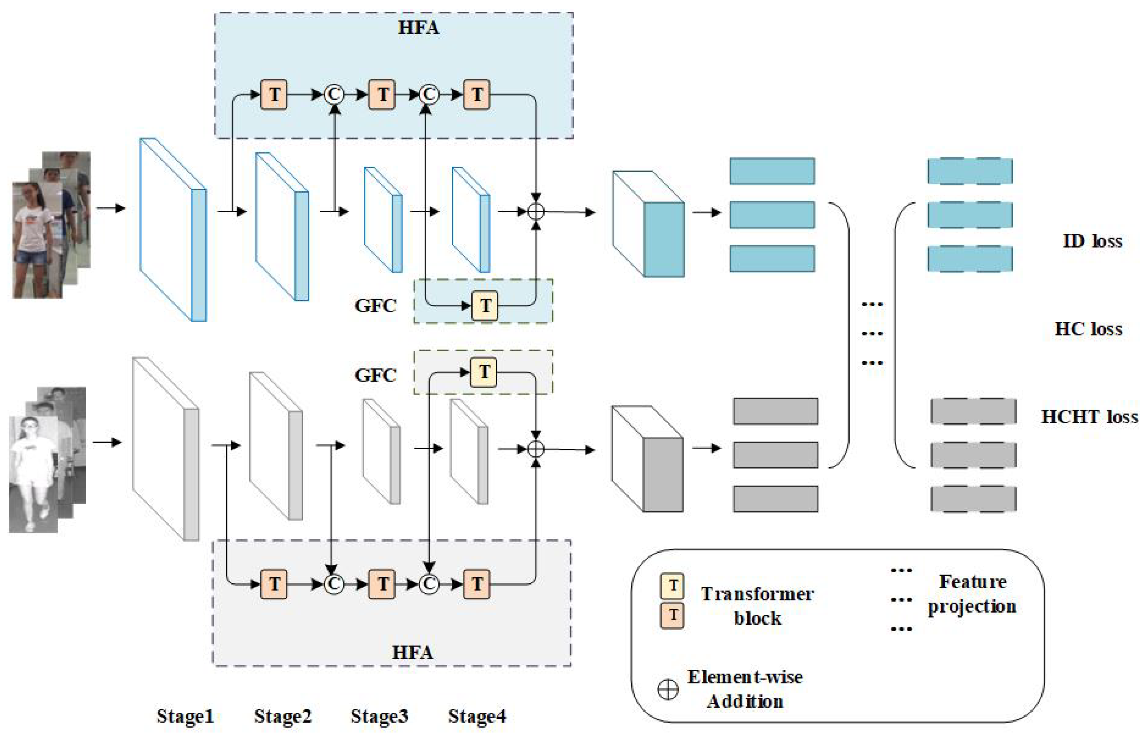
Analysis of each component: Our method consists of four components: a baseline network, HFA, GFC, and heterogeneous-center hard triplet loss. We chose TSLFN [45] as the baseline, which is a two-stream network supervised jointly with cross-entropy loss and heterogeneous-center loss. The baseline is denoted as “B”, while HFA is denoted as “A”, GFC is indicated as “C”, and the heterogeneous-center hard triplet loss is denoted as “L”.

Table 1. Experimental results for different components on the SYSU-MM01 dataset (all-search mode). Showing the values of rank-r and mAP (%).

Method	Rank-1	Rank-10	Rank-20	mAP
B	54.85	89.65	97.42	55.88
B+A	58.80	93.32	97.77	58.10
B+C	58.75	92.96	97.57	57.43
B+A+C	59.29	93.77	98.04	57.76
B+A+C+L	60.87	93.58	98.37	58.87

The bold represents the best performance.

shows the experimental results. The rank-1 and mAP of the baseline network are 54.85% and 55.88%, respectively. Adding the HFA module alone, rank-1 and mAP increased by 3.95% and 2.22%, respectively. Adding the GFC module alone, the rank-1 and mAP increased by 3.9% and 1.55%, respectively. This phenomenon proves the effectiveness of enriching deep features with detailed information and globally compensating for features. After combining the two modules, noteworthy enhancements in the network’s performance were observed, underscoring the mutually reinforcing nature of the HFA and GFC modules. Finally, we added the HCHT to the previous ones. The values of rank-1 and mAP reached 60.23% and 58.48%, respectively.

Parameter analysis of HFA: To analyze the validity of the HFA module, we performed comparative experiments on different combinations of aggregating hierarchical features. Meanwhile, we also analyzed the number of layers of each Transformer (the results are shown in

Table 2. Ablation experiments of parameters of HFA on the SYSU-MM01 dataset (all-search mode). Showing the values of rank-r and mAP (%).

Index	Method	Rank-1	Rank-10	Rank-20	mAP
1	{3,3,3,3}	32.78	76.26	86.87	33.94
2	{0,4,4,4}	43.02	84.05	91.16	42.53
3	{4,4,4,0}	57.61	93.00	97.68	57.00
4	{3,4,5,0}	57.30	92.96	97.54	56.61
5	{3,3,6,0}	57.64	93.10	97.91	57.16
6	{3,2,7,0}	58.31	93.31	97.81	57.35
7	{3,1,8,0}	58.80	93.32	97.77	58.10
8	{2,1,9,0}	57.99	93.21	97.82	57.33

The bold represents the best performance.

). In $\{n_1,n_2,\dots ,n_n\}$, $n_i(i=1,2,3,4)$ represents the number of Transformer layers added after the i-th stage. $n_i=0$ means that the hierarchical features of the i-th stage do not participate in the aggregation process. According to the setting in ViT [42], we fixed the total layers of all Transformer blocks in HFA at 12 and the heads of each Transformer encoder at 16.

The experimental results of the first three groups show that it is not wise to let the hierarchical features of the four stages participate in the aggregation process. We infer that blindly integrating all the features will make the information too messy and overlapping, resulting in a burden to the network. Comparing the experimental results of the second and third group, we find that the effect of aggregating the hierarchical features from stage 2 to stage 4 is not ideal. The reason may be that, in the process of stage 1 to stage 4, the features extracted by the network contain less and less detailed information but more and more semantic information. This leads to shallow features with more details and less semantic information and to deep features with fewer details and more semantic information. If we choose to aggregate hierarchical features at a high level, the semantic information is enough, but the detailed information is mostly lost. Thus, we deduce that the low performance is caused by the loss of detailed information.

Comparing the experimental results of the third to seventh group, we find a very interesting phenomenon. When $Tranforme{r}_2$ has fewer layers and $Tranforme{r}_3$ has more layers, the performance is better. The optimal values of rank-1 and mAP reached 58.80% and 58.10%, respectively. The reason may be that semantic information is more advanced and complex than detailed information, so more layers are needed to process it. Comparing the experimental results of the last two groups, we find that blindly increasing the number of layers of $Tranforme{r}_3$ will lead to performance degradation. We infer that the accuracy tends to converge as the depth of the Transformer increases. Finally, the performance is best when the depths of $Tranforme{r}_1$, $Tranforme{r}_2$, and $Tranforme{r}_3$ are 3, 1, and 8, respectively.

Parameter analysis of GFC: To analyze the validity of the GFC module, we performed comparative experiments on the settings of $Tranforme{r}_4$. Considering the burden of the entire network, we chose a Transformer with a relatively simple setting. Experimental results are detailed in

Table 3. Experimental results of different settings of GFC on the SYSU-MM01 dataset (all-search mode). Showing the values of rank-r and mAP (%).

Heads	Depth	Rank-1	Rank-10	Rank-20	mAP
1	1	56.85	92.02	97.24	55.59
1	2	57.25	93.05	97.94	56.49
2	1	57.19	93.10	97.82	56.58
2	2	58.15	93.16	97.92	56.89
4	1	58.75	92.96	97.57	57.43
4	2	56.93	92.42	97.47	55.63
8	1	58.74	92.92	97.65	57.50
8	2	56.93	92.19	97.24	55.39

The bold represents the best performance.

. When the number of heads is 4 and the depth is 1, rank-1 and mAP are optimal, 58.75% and 57.43%, respectively. Observing the overall results in Table 3, there is a rule that, as the number of heads increases, the performance constantly improves. This phenomenon shows that the more heads the Transformer has, the stronger its ability to process features, and the more discriminative global features it can extract. We notice that when the number of heads is 4 and 8, their results are very close. In response to this phenomenon, we deduce that the accuracy tends to converge as the number of heads increases.

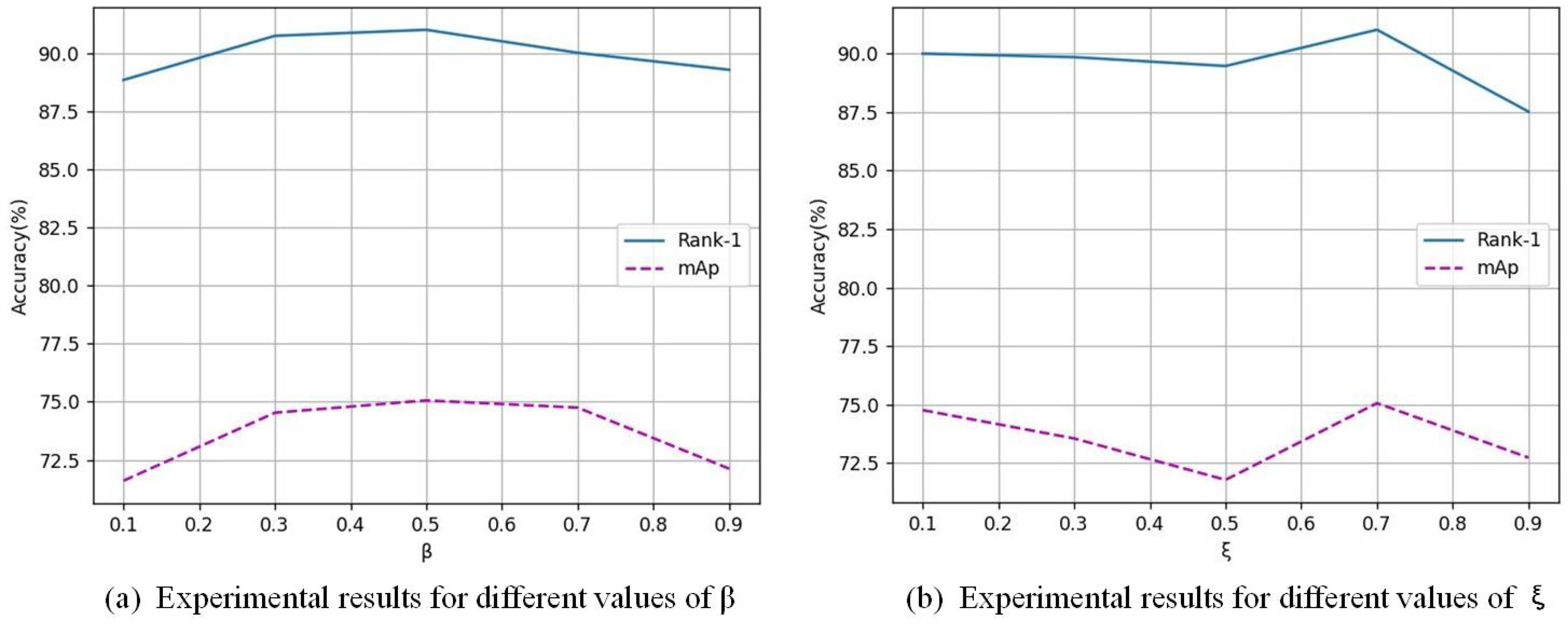
Analysis of parameters $\beta$ and $\xi$: In this part, we explore the influence of $\beta$ and $\xi$ in the loss function. This experiment was performed on a network with HFA and GFC modules added. First, we kept the value of $\xi$ at 0.7 and increased the value of $\beta$ from 0.1 to 0.9. Figure 3a shows that, when $\beta$ = 0.5, the result reaches the best level. Secondly, we changed $\xi$ regularly from 0.1 to 0.9. Figure 3b shows that, when $\xi$ = 0.7, the performance is optimal, and the rank-1 and mAP reach 91.02% and 75.06%, respectively. When the value of $\xi$ is too large, the performance drops significantly. We infer that this is due to the network’s difficulty in balancing the distances between different identities.

Comparison of different backbones: The proposed TFCNet uses ResNet50 as the backbone and embeds multiple Transformer blocks in it. Considering that this structure may be costly, we adjusted it to use Transformer as the backbone. The results are shown in

Table 4. Comparison of different backbones on the SYSU-MM01 dataset. Showing the values of rank-r and mAP (%).

Backbone	All-Search				Indoor-Search
	R-1	R-10	R-20	mAP	R-1	R-10	R-20	mAP
ResNet50	60.87	93.58	98.37	58.87	63.59	95.67	98.68	70.28
Transformer	53.85	92.24	96.84	52.85	59.83	93.39	97.83	67.78

The bold represents the best performance.

and

Table 5. Comparison of different backbones on the REGDB dataset under both settings. Showing the values of rank-r and mAP (%).

Backbone	Visible → Infrared				Infrared → Visible
	R-1	R-10	R-20	mAP	R-1	R-10	R-20	mAP
ResNet50	91.02	98.25	99.37	75.06	90.39	97.82	98.69	74.68
Transformer	74.17	90.49	94.37	68.69	70.97	89.42	94.03	66.72

The bold represents the best performance.

. We find that using Transformer as the backbone actually degrades the model’s performance. The reason may be that the four stages of ResNet50 are crucial for the extraction of semantic information, and it is not recommended to replace them with a series of simple convolution blocks. Specifically, our method uses the lost detail information to assist the semantic information in improving performance. In this process, semantic information dominates, and detailed information only plays a supporting role. However, in a network with Transformer as the backbone, the extraction of semantic information only relies on a series of simple convolution blocks, which may result in poor quality and small quantity of semantic information, thus reducing performance.

4.3. Analysis of the HFA Module

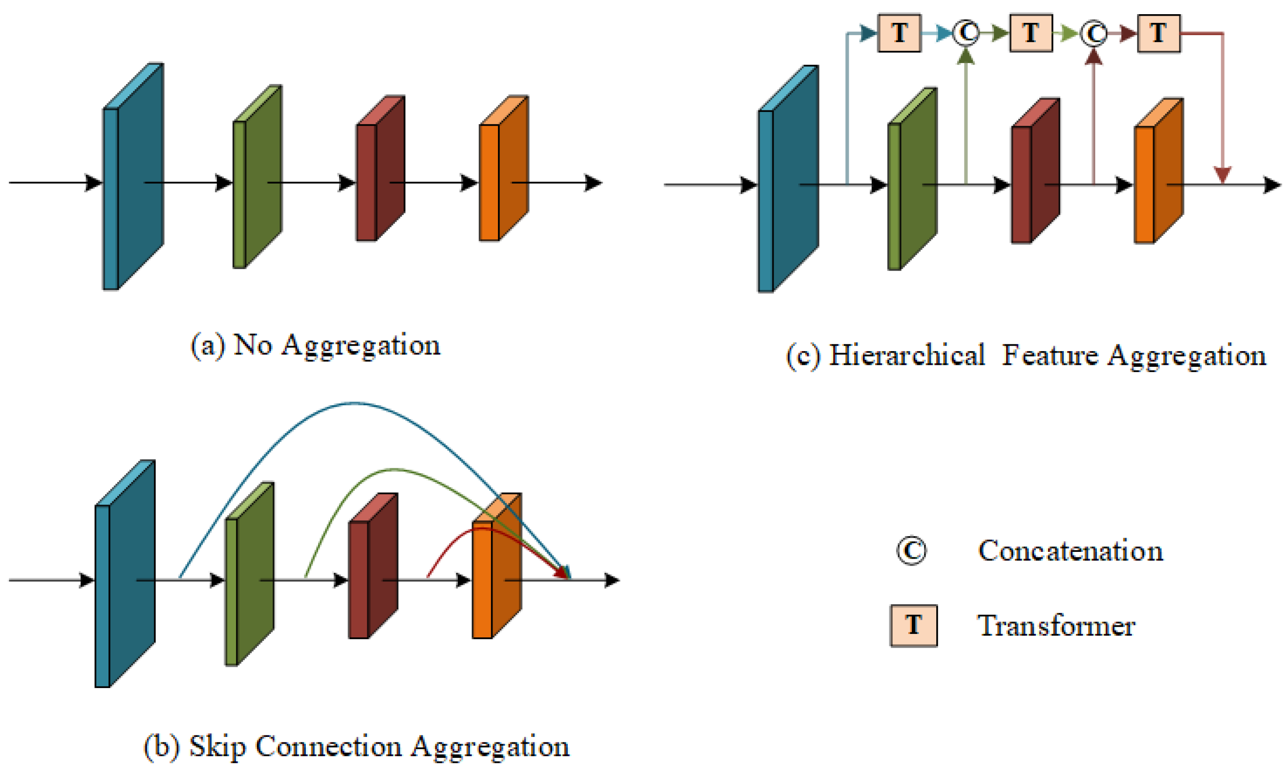
Comparison of feature aggregation methods: Skip connection is the most common method for aggregating multiple features at the same time. From Figure 4b, we can see that this method is simple and crude, directly concatenating shallow-level, middle-level, and deep-level features. We replace hierarchical feature aggregation with skip connection aggregation in our model. By observing the results in

Table 6. Experimental results of different feature aggregation methods on the SYSU-MM01 dataset (all-search mode). Showing the values of rank-r and mAP (%).

Method	Rank-1	Rank-10	Rank-20	mAP
(a)	54.85	89.65	97.42	55.88
(b)	56.32	92.37	97.29	55.94
(c)	58.80	93.32	97.77	58.10

The bold represents the best performance.

, we find that, whether we use skip connection aggregation or hierarchical feature aggregation, the model performance is significantly improved. However, the hierarchical feature aggregation is obviously better, being 2.48 points higher than the skip connection aggregation. This is due to the fact that simple aggregation operations of shallow and deep features will limit performance. To ensure the accuracy and fairness of the comparison, the three methods in Table 6 all use the same losses, namely ID loss and HC loss.

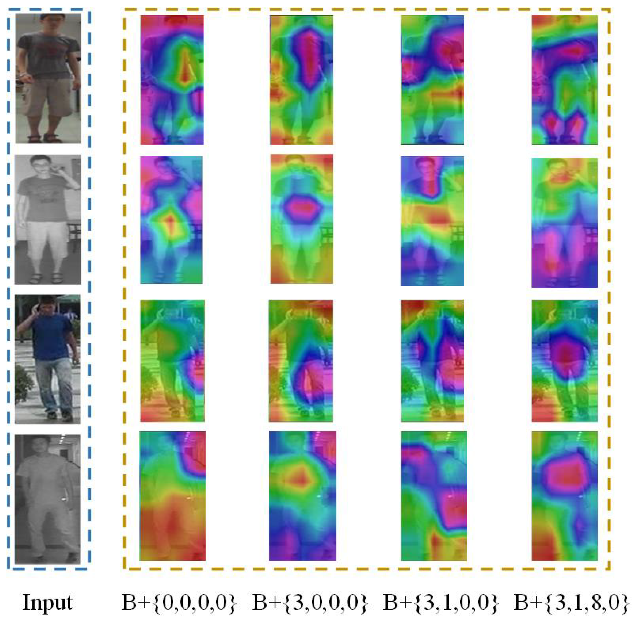
Analysis of the effectiveness of each Transformer: We compare four sets of experiments to confirm its effectiveness: without adding a Transformer encoder, adding a Transformer encoder after stage 1, adding it after stage 1∼stage 2, and adding it after stage 1∼stage 3. The results are shown in

Table 7. Analysis of the effectiveness of each Transformer in HFA on the SYSU-MM01 dataset (all-search mode). Showing the values of rank-r and mAP (%).

Method	Rank-1	Rank-10	Rank-20	mAP
B	54.85	89.65	97.42	55.88
B+{3,0,0,0}	57.89	93.11	97.56	56.72
B+{3,1,0,0}	58.56	92.64	97.48	57.44
B+{3,1,8,0}	58.80	93.32	97.77	58.10

The bold represents the best performance.

. We find that the rank-1/mAP of these four sets of experiments shows an upward trend, which affirms the idea of enriching features with detailed information to improve performance. Meanwhile, we calculate the rank-1/mAP increments between the four experiments, which are 3.04%/0.84%, 0.67%/0.72%, and 0.24%/0.66%, respectively. The results show that the increment between the second and first set of experiments is the largest. Because shallow features have more detailed information, Transformer extracts and transfers them to deep features, which can greatly improve model performance. Comparing the third and fourth group of experiments, although their results are improving, the increments are not obvious. This is because, as the number of convolutions increases, the features contain fewer and fewer details.

4.4. Visualization Analysis

Heatmap visualization: To more intuitively demonstrate the effectiveness of each Transformer in HFA, we conducted a heatmap visualization experiment. The experiment follows the settings in the previous section, and the results are shown in Figure 5. By observing the heatmaps of the baseline, we find that the high response is concentrated in the background area. However, after gradually adding Transformer encoders, the problem is alleviated. As can be seen from the last three columns of Figure 5, high responses are increasingly concentrated in body parts. This illustrates the effectiveness of detailed information for pedestrian learning.

Feature distribution: To prove the effectiveness of enriching deep features with detailed information and global compensation for features during feature extraction, we conducted distribution visualization experiments on visible features. According to Figure 6a, we can clearly see that the baseline network has serious problems of overlapping distribution of different identity features and scattered distribution of the same identity features. However, our network alleviates these problems very well.

4.5. Comparison with State-of-the-Art Methods

Within this subsection, we conduct a comparative analysis of the proposed approach against state-of-the-art methods on the SYSU-MM01 and RegDB datasets. All methods use the ResNet-50 network as the backbone. The comparison methods are split into two categories, namely modality transformation-based methods and feature learning-based methods. D${}^2$RL [35], AlignGAN [34], Hi-CMD [3], and XIV [4] reduce cross-modality discrepancy through image generation techniques. For example, AlignGAN [34] converts visible images into corresponding infrared images through CycleGAN to solve the issue of cross-modality discrepancies. DDAG [1], AGW [2], DLS [6], NFS [5], PIC [47], and DFLN-ViT [48] reduce cross-modality discrepancy by extracting discriminative modality-shared features. For example, DFLN-ViT [48] considers potential correlations between different locations and channels.

SYSU-MM01 dataset:

Table 8. Comparison with the state-of-art methods on the SYSU-MM01 dataset. Showing the values of rank-r and mAP (%).

Methods	Publication	All-Search		Indoor-Search
		R-1	mAP	R-1	mAP
Zero-Pad [31]	ICCV17	14.80	15.95	20.58	26.92
HCML [32]	AAAI18	14.32	16.16	24.52	30.08
BDTR [33]	IJCAI18	17.01	19.66	-	-
cmGAN [36]	IJCAI18	26.97	27.80	31.63	42.19
D${}^2$RL [35]	CVPR19	28.90	29.20	-	-
AlignGAN [34]	ICCV19	42.40	40.70	45.90	54.30
Hi-CMD [3]	CVPR20	34.94	35.94	-	-
XIV [4]	AAAI20	49.92	50.73	-	-
DDAG [1]	ECCV20	54.75	53.02	61.02	67.98
AGW [2]	TPAMI21	47.50	47.65	54.17	62.97
DLS [6]	TMM21	48.80	49.00	-	-
NFS [5]	CVPR21	56.91	55.45	62.79	69.79
PIC [47]	TIP22	57.50	55.10	60.40	67.70
DFLN-ViT [48]	TMM22	57.65	55.96	60.58	67.28
TFCNet	-	60.87	58.87	63.59	70.28

The bold represents the best performance.

shows the comparison results, and our proposed method reaches the optimum. Specifically, our rank-1/mAP achieves 60.87%/58.87% and 63.59%/70.28% for the two search modes, respectively. Comparing with the modality transformation-based method [4], the rank-1/mAP of TFCNet is 10.95%/8.14% higher than it is in the all-search mode. This shows that our method can achieve good results without the additional cost of image generation. Comparing with the feature learning-based method [48], the rank-1/mAP of TFCNet is 3.22%/2.91% and 3.01%/3% higher than it is in the two settings, respectively. This shows the effectiveness of enriching deep features with detailed information and global compensation for local features with Transformer.

RegDB dataset:

Table 9. Comparison with state-of-art methods on the RegDB dataset under both settings. Showing the values of rank-r and mAP (%).

Methods	Publication	All-Search		Indoor-Search
		R-1	mAP	R-1	mAP
Zero-Pad [31]	ICCV17	17.74	18.90	16.63	17.82
HCML [32]	AAAI18	24.44	20.08	21.70	22.24
BDTR [33]	IJCAI18	33.47	31.83	-	-
D${}^2$RL [35]	CVPR19	43.40	44.10	-	-
AlignGAN [34]	ICCV19	57.90	53.60	56.30	53.40
Hi-CMD [3]	CVPR20	70.93	66.04	-	-
XIV [4]	AAAI20	62.21	60.18	-	-
DDAG [1]	ECCV20	69.34	63.46	68.06	61.80
AGW [2]	TPAMI21	70.05	66.37	-	-
DLS [6]	TMM21	71.10	68.10	-	-
NFS [5]	CVPR21	80.54	72.10	77.95	69.79
PIC [47]	TIP22	83.60	79.60	79.50	77.40
DFLN-ViT [48]	TMM22	89.03	76.24	88.83	74.93
TFCNet	-	91.02	75.06	90.39	74.68

The bold represents the best performance.

shows the comparison results. The rank-1/mAP of our TFCNet reaches 91.02%/75.06% and 90.39%/74.68% under the two settings, respectively. Compared with the modality transformation-based method [3], the rank-1/mAP of TFCNet is 20.09%/9.02% higher than it is in visible-to-infrared mode. Comparing with the feature learning-based method [48], the rank-1 of TFCNet outperforms it by 1.99% and 1.56% in two settings, respectively. The rank-1 of our method is the highest. Although the value of mAP is not optimal, it is not much different from the value of the optimal method. The effectiveness of the designed network can also be demonstrated on this dataset.

It should be noted that the results of DFLN-ViT [48] in Table 8 and Table 9 are inconsistent with the original paper. This is because we reproduced it on an NVIDIA 3090 GPU and filled the tables with the results of the reproduction.

4.6. Migration Experiments on Remote Sensing Datasets

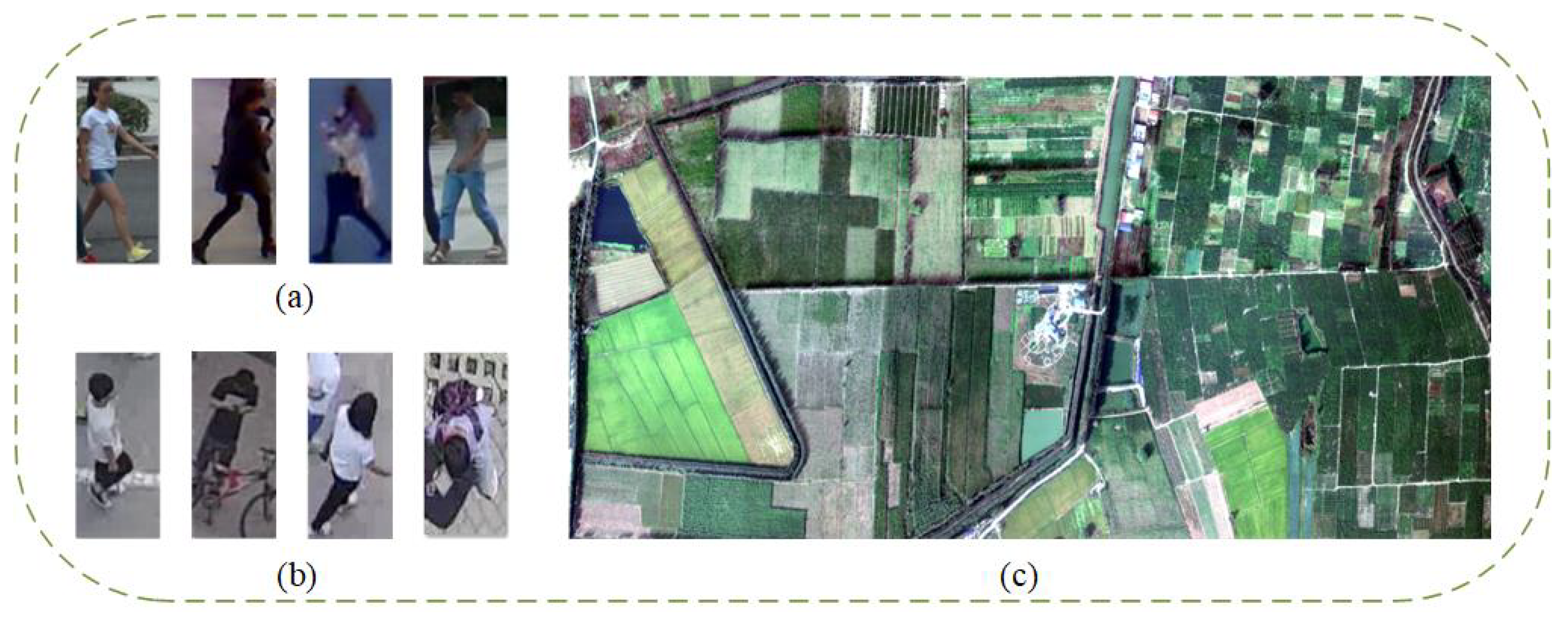
From Figure 7, we can see that aerial pictures have a smaller field of view and less valuable information than those taken by traditional fixed cameras, which requires the network to have a higher degree of control over detailed information. Since our proposed HFA module involves detailed information, we only show the heatmap visualization of each Transformer encoder in the HFA model when conducting migration experiments on remote sensing datasets. Meanwhile, considering that the PRAI-1581 and Matiwan Village datasets are in the RGB modality, we only retain the visible branch of TFCNet.

PRAI-1581 dataset: The experimental results of our method on the PRAI-1581 dataset are shown in

Table 10. Comparison with other methods on the PRAI-1581 dataset. Showing the values of rank-r and mAP (%).

Method	Publication	mAP	Rank-1
SVDNet [49]	ICCV17	36.70	46.10
PCB+RPP [50]	ECCV18	38.45	48.07
OSNET [51]	ICCV19	42.10	54.40
Ours	-	45.25	56.40

The bold represents the best performance.

, where rank-1/mAP reached 45.25%/56.40%. The results are 8.55%/10.3%, 6.8%/8.33%, and 3.15%/2% higher than SVDNet [49], PCB+RPP [50], and OSNET [51] respectively, which proves that our method has good transferability and effectiveness.

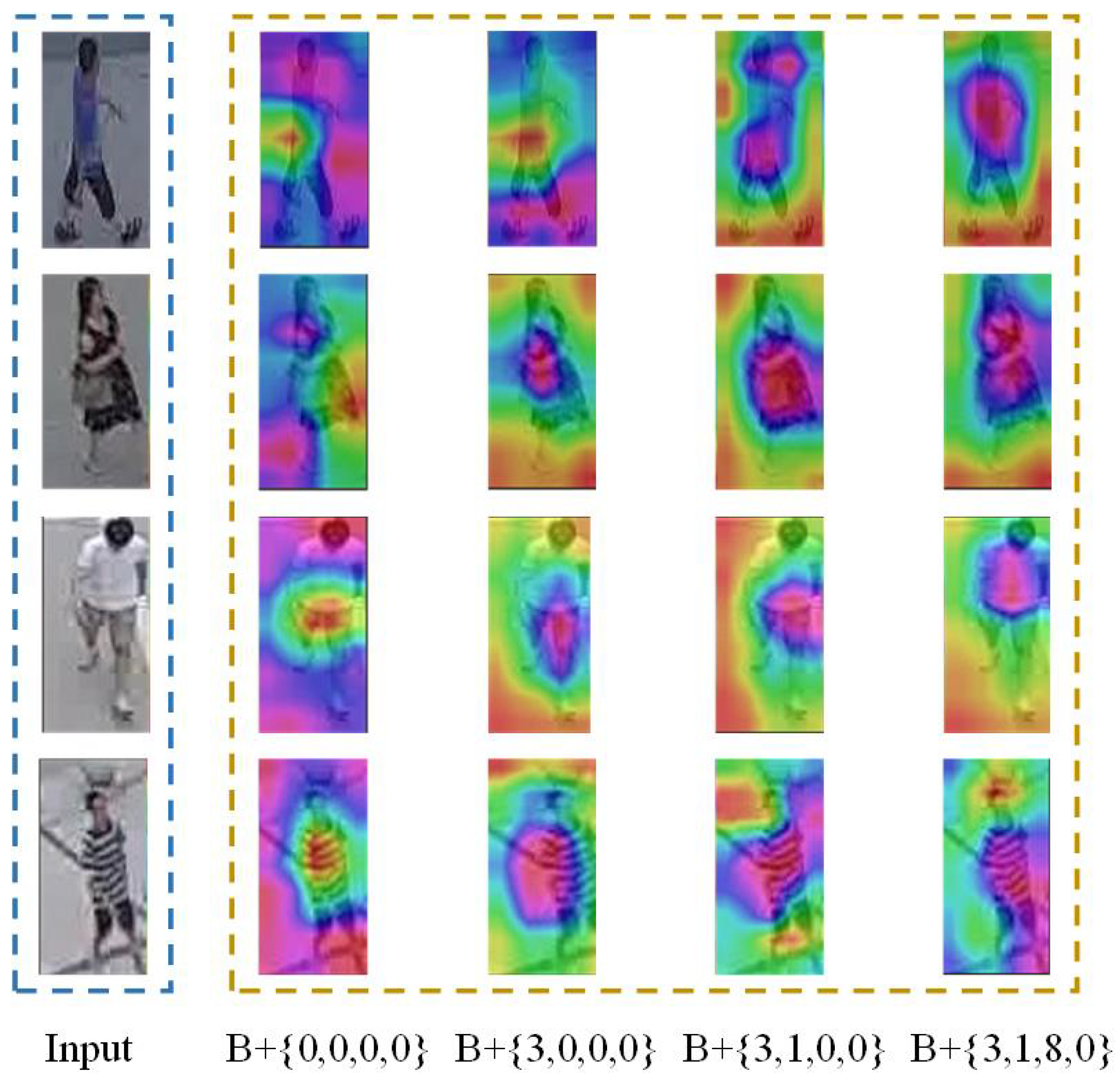
Due to the limitations of aerial images, more attention needs to be paid to detailed information. The HFA module of our method solves the problem of detailed information loss in the feature extraction process. Therefore, to prove the effectiveness of the HFA module on aerial images, we conducted heatmap visualization experiments for each Transformer encoder. The outcomes are depicted in Figure 8. We find that, as the number of Transformer encoders increases, the high response becomes more and more concentrated in the body parts.

We randomly seleced four images from the dataset, and the Top-10 retrieval results are shown in Figure 9. As can be seen, only a few images match correctly. These erroneous images are very similar to the query image and can be mainly attributed to the similar appearance of different pedestrians caused by the aerial photography angle and altitude.

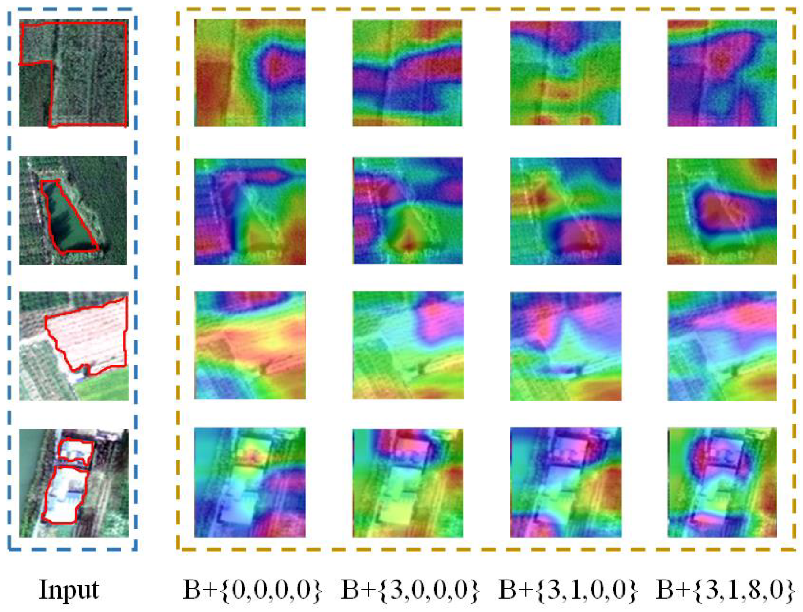
Matiwan Village dataset: Figure 7c is the overall aerial picture of Matiwan Village, which contains 19 categories of features. We selected four of them (willow trees, water bodies, grasslands, and houses) for study. To showcase the efficacy of the HFA module across these categories, we conducted heatmap visualization experiments for each Transformer encoder. The specific results are shown in Figure 10. We found that, as the number of Transformer encoders increases, high responses are increasingly concentrated in areas that need to be recognized. This proves that our method is good at identifying pedestrians and can be transferred to other targets.

4.7. Advantages of Cosine Similarity Image Matching Algorithm

The image matching algorithm selected in our method is the cosine similarity matching algorithm, which has the following four advantages:

• Direction invariance: Cosine similarity is invariant to changes in image direction and can cope well with the problem of object/pedestrian direction differences in remote sensing images/pedestrian images.
• Scale invariance: Cosine similarity has certain invariance to changes in image scale and can cope well with the problem of object/pedestrian scale differences in remote sensing images/pedestrian images.
• Intuitive interpretability: The cosine similarity value range spans from −1 to 1, where 1 means completely similar and −1 means completely different. This representation enables a visual representation of the matching results.
• Efficient calculation: The calculation of cosine similarity only involves the dot product and module length calculation between feature vectors. This efficient calculation can speed up the image matching process and improve efficiency.

5. Conclusions

This paper aimed to design a network for VI-ReID. The proposed network mainly consists of a Hierarchical Feature Aggregation (HFA) module and a Global Feature Compensation (GFC) module. HFA recursively aggregates the hierarchical features of the CNN backbone to help the model preserve detailed information. GFC exploits the Transformer’s ability to model long-range dependencies on spatial and sequential data to compensate for the CNN’s issue with capturing global representations. Moreover, we jointly apply ID loss, heterogeneous-center loss, and heterogeneous-center hard triplet loss to train the feature extraction process. The achieved results on two cross-modality datasets, namely SYSU-MM01 and RegDB, exhibit accuracies of 60.87% and 91.02%, respectively, indicating that our method outperforms most state-of the-art methods. Moreover, experimental results on two aerial photography datasets also prove that our method has good transferability.

References

1. Ye, M.; Shen, J.; Crandall, D.; Shao, L.; Luo, J. Dynamic dual-attentive aggregation learning for visible-infrared person re-identification. In Proceedings of the European Conference on Computer Vision, Online, 23–28 August 2020; pp. 229–247. [Google Scholar]
2. Ye, M.; Shen, J.; Lin, G.; Xiang, T.; Shao, L.; Hoi, S. Deep learning for person re-identification: A survey and outlook. IEEE Trans. Pattern Anal. Mach. Intell. 2021, 44, 2872–2893. [Google Scholar] [CrossRef] [PubMed]
3. Choi, S.; Lee, S.; Kim, Y.; Kim, T.; Kim, C. Hi-CMD: Hierarchical cross-modality disentanglement for visible-infrared person re-identification. In Proceedings of the IEEE/CVF Conference on Computer Vision and Pattern Recognition, Seattle, WA, USA, 13–19 June 2020; pp. 10257–10266. [Google Scholar]
4. Li, D.; Wei, X.; Hong, X.; Gong, Y. Infrared-visible cross-modal person re-identification with an X modality. In Proceedings of the AAAI Conference on Artificial Intelligence, New York, NY, USA, 7–12 February 2020; Volume 34, pp. 4610–4617. [Google Scholar]
5. Chen, Y.; Wan, L.; Li, Z.; Jing, Q.; Sun, Z. Neural feature search for RGB-infrared person re-identification. In Proceedings of the IEEE/CVF Conference on Computer Vision and Pattern Recognition, Nashville, TN, USA, 20–25 June 2021; pp. 587–597. [Google Scholar]
6. Huang, Y.; Wu, Q.; Xu, J.; Zhong, Y.; Zhang, P.; Zhang, Z. Alleviating modality bias training for infrared-visible person re-identification. IEEE Trans. Multimed. 2021, 24, 1570–1582. [Google Scholar] [CrossRef]
7. Zhang, S.; Zhang, Q.; Yang, Y.; Wei, X.; Wang, P.; Jiao, B.; Zhang, Y. Person re-identification in aerial imagery. IEEE Trans. Multimed. 2020, 23, 281–291. [Google Scholar] [CrossRef]
8. Cen, Y.; Zhang, L.; Zhang, X.; Wang, Y.; Qi, W.; Tang, S.; Zhang, P. Aerial hyperspectral remote sensing classification dataset of Xiongan New Area (Matiwan Village). Natl. Remote Sens. Bull. 2020, 24, 1299–1306. [Google Scholar]
9. Leng, Q.; Ye, M.; Tian, Q. A survey of open-world person re-identification. IEEE Trans. Circuits Syst. Video Technol. 2020, 30, 1092–1108. [Google Scholar] [CrossRef]
10. Ye, M.; Shen, J. Probabilistic structural latent representation for unsupervised embedding. In Proceedings of the IEEE/CVF Conference on Computer Vision and Pattern Recognition, Seattle, WA, USA, 13–19 June 2020; pp. 5456–5465. [Google Scholar]
11. Zhang, G.; Chen, Y.; Lin, W.; Chandran, A.; Xuan, J. Low Resolution Information Also Matters: Learning Multi-Resolution Representation for Person Re-identification. In Proceedings of the International Joint Conference on Artificial Intelligence, Montreal, QC, Canada, 19–26 August 2021; pp. 1295–1301. [Google Scholar]
12. Ye, Q.; Huang, P.; Zhang, Z.; Zheng, Y.; Fu, L.; Yang, W. Multiview learning with robust double-sided twin SVM. IEEE Trans. Cybern. 2021, 52, 12745–12758. [Google Scholar] [CrossRef] [PubMed]
13. Zhang, G.; Ge, Y.; Dong, Z.; Wang, H.; Zheng, Y.; Chen, S. Deep High-Resolution Representation Learning for Cross-Resolution Person Re-identification. IEEE Trans. Image Process. 2021, 30, 8913–8925. [Google Scholar] [CrossRef]
14. Loy, C.; Xiang, T.; Gong, S. Multi-camera activity correlation analysis. In Proceedings of the IEEE/CVF Conference on Computer Vision and Pattern Recognition, Miami, FL, USA, 20–25 June 2009; pp. 1988–1995. [Google Scholar]
15. Kostinger, M.; Hirzer, M.; Wohlhart, P.; Roth, P.; Bischof, H. Large scale metric learning from equivalence constraints. In Proceedings of the IEEE/CVF Conference on Computer Vision and Pattern Recognition, Nashville, TN, USA, 20–25 June 2021; pp. 2288–2295. [Google Scholar]
16. Fu, L.; Li, Z.; Ye, Q.; Yin, H.; Liu, Q.; Chen, X.; Fan, X.; Yang, W.; Yang, G. Learning Robust Discriminant Subspace Based on Joint L2,p- and L2,s-Norm Distance Metrics. IEEE Trans. Neural Netw. Learn. Syst. 2022, 33, 130–144. [Google Scholar] [CrossRef]
17. Zhang, G.; Fang, W.; Zheng, Y.; Wang, R. SDBAD-Net: A Spatial Dual-Branch Attention Dehazing Network based on Meta-Former Paradigm. IEEE Trans. Circuits Syst. Video Technol. 2023, 34, 60–70. [Google Scholar] [CrossRef]
18. Zhang, G.; Liu, J.; Chen, Y.; Zheng, Y.; Zhang, H. Multi-biometric Unified Network for Cloth-changing Person Re-Identification. IEEE Trans. Image Process. 2023, 32, 4555–4566. [Google Scholar] [CrossRef]
19. Saber, S.; Amin, K.; Pławiak, P.; Tadeusiewicz, V.; Hammad, M. Graph convolutional network with triplet attention learning for person re-identification. Inf. Sci. 2022, 617, 331–345. [Google Scholar] [CrossRef]
20. Wang, J.; Yuan, L.; Xu, H.; Xie, G.; Wen, X. Channel-exchanged feature representations for person re-identification. Inf. Sci. 2021, 562, 370–384. [Google Scholar] [CrossRef]
21. Zheng, W.; Gong, S.; Xiang, T. Person re-identification by probabilistic relative distance comparison. In Proceedings of the IEEE/CVF Conference on Computer Vision and Pattern Recognition, Colorado Springs, CO, USA, 20–25 June 2011; pp. 649–656. [Google Scholar]
22. Li, Z.; Chang, S.; Liang, F.; Huang, T.; Cao, L.; Smith, J. Learning locally adaptive decision functions for person verification. In Proceedings of the IEEE/CVF Conference on Computer Vision and Pattern Recognition, Portland, OR, USA, 23–28 June 2013; pp. 3610–3617. [Google Scholar]
23. Zhang, G.; Zhang, H.; Lin, W.; Chandran, A.; Jing, X. Camera Contrast Learning for Unsupervised Person Re-Identification. IEEE Trans. Circuits Syst. Video Technol. 2023, 33, 4096–4107. [Google Scholar] [CrossRef]
24. Liao, S.; Hu, Y.; Zhu, X.; Li, S. Person re-identification by local maximal occurrence representation and metric learning. In Proceedings of the IEEE/CVF Conference on Computer Vision and Pattern Recognition, Boston, MA, USA, 7–12 June 2015; pp. 2197–2206. [Google Scholar]
25. Chen, Y.; Zhang, G.; Lu, Y.; Wang, Z.; Zheng, Y. A Simple but Effective Part-based Convolutional Baseline for Text-based Person Search. Neurocomputing 2022, 494, 171–181. [Google Scholar] [CrossRef]
26. Li, W.; Zhu, X.; Gong, S. Harmonious attention network for person re-identification. In Proceedings of the IEEE/CVF Conference on Computer Vision and Pattern Recognition, Salt Lake City, UT, USA, 18–23 June 2018; pp. 2285–2294. [Google Scholar]
27. Yang, F.; Yan, K.; Lu, S.; Jia, H.; Xie, X.; Gao, W. Attention driven person re-identification. Pattern Recognit. 2019, 86, 143–155. [Google Scholar] [CrossRef]
28. Zhang, G.; Luo, Z.; Chen, Y.; Zheng, Y.; Lin, W. Illumination Unification for Person Re-identification. IEEE Trans. Circuits Syst. Video Technol. 2022, 32, 6766–6777. [Google Scholar] [CrossRef]
29. Feng, Y.; Yu, J.; Chen, F.; Ji, Y.; Wu, F.; Liu, S.; Jing, X. Visible-Infrared Person Re-Identification via Cross-Modality Interaction Transformer. IEEE Trans. Multimed. 2022, 25, 7647–7659. [Google Scholar] [CrossRef]
30. Zhang, H.; Zhang, G.; Chen, Y.; Zheng, Y. Global relation-aware contrast learning for unsupervised person re-identification. IEEE Trans. Circuits Syst. Video Technol. 2022, 32, 8599–8610. [Google Scholar] [CrossRef]
31. Wu, A.; Zheng, W.; Yu, H.; Gong, S.; Lai, J. Rgb-infrared cross-modality person re-identification. In Proceedings of the IEEE International Conference on Computer Vision, Venice, Italy, 22–29 October 2017; pp. 5380–5389. [Google Scholar]
32. Ye, M.; Lan, X.; Li, J.; Yuen, P. Hierarchical discriminative learning for visible thermal person re-identification. Proc. AAAI Conf. Artif. Intell. 2018, 32, 7501–7508. [Google Scholar] [CrossRef]
33. Ye, M.; Wang, Z.; Lan, X.; Yuen, P. Visible thermal person re-identification via dual-constrained top-ranking. In Proceedings of the Twenty-Seventh International Joint Conference on Artificial Intelligence, Stockholm, Sweden, 13–19 July 2018; pp. 1092–1099. [Google Scholar]
34. Wang, G.; Zhang, T.; Cheng, J.; Liu, S.; Yang, Y.; Hou, Z. RGB-infrared cross-modality person re-identification via joint pixel and feature alignment. In Proceedings of the IEEE International Conference on Computer Vision, Seoul, Republic of Korea, 27 October–2 November 2019; pp. 3623–3632. [Google Scholar]
35. Wang, Z.; Wang, Z.; Zheng, Y.; Chuang, Y.; Satoh, S. Learning to reduce dual-level discrepancy for infrared-visible person re-identification. In Proceedings of the IEEE/CVF Conference on Computer Vision and Pattern Recognition, Long Beach, CA, USA, 15–20 June 2019; pp. 618–626. [Google Scholar]
36. Dai, P.; Ji, R.; Wang, H.; Wu, Q.; Huang, Y. Cross-Modality Person Re-Identification with Generative Adversarial Training. In Proceedings of the Twenty-Seventh International Joint Conference on Artificial Intelligence, Stockholm, Sweden, 13–19 July 2018; pp. 677–683. [Google Scholar]
37. Lippitt, C.; Zhang, S. The impact of small unmanned airborne platforms on passive optical remote sensing: A conceptual perspective. Int. J. Remote. Sens. 2018, 39, 4852–4868. [Google Scholar] [CrossRef]
38. Zhang, S.; Bogus, S.; Lippitt, C.; Kamat, V.; Lee, S. Implementing remote-sensing methodologies for construction research: An unoccupied airborne system perspective. J. Constr. Eng. Manag. 2022, 148, 03122005. [Google Scholar] [CrossRef]
39. Bouhlel, F.; Mliki, H.; Hammami, M. Suspicious Person Retrieval from UAV-sensors based on part level deep features. Procedia Comput. Sci. 2021, 192, 318–327. [Google Scholar] [CrossRef]
40. Mei, X.; Pan, E.; Ma, Y.; Dai, X.; Huang, J.; Fan, F.; Du, Q.; Zheng, H.; Ma, J. Spectral-spatial attention networks for hyperspectral image classification. Remote Sens. 2019, 11, 963. [Google Scholar] [CrossRef]
41. Vaswani, A.; Shazeer, N.; Parmar, N.; Uszkoreit, J.; Jones, V.; Gomez, A.; Kaiser, Ł.; Polosukhin, I. Attention is all you need. Adv. Neural Inf. Process. Syst. 2017, 30. Available online: https://proceedings.neurips.cc/paper/2017/file/3f5ee243547dee91fbd053c1c4a845aa-Paper.pdf (accessed on 24 November 2023).
42. Dosovitskiy, A.; Beyer, L.; Kolesnikov, A.; Weissenborn, D.; Zhai, X.; Unterthiner, T.; Dehghani, M.; Heigold, G.; Gelly, S. An Image is Worth 16 × 16 Words: Transformers for Image Recognition at Scale. In Proceedings of the International Conference on Learning Representations, Vienna, Austria, 3–7 May 2021. [Google Scholar]
43. Zhu, Y.; Yang, Z.; Wang, L.; Zhao, S.; Hu, X.; Tao, D. Hetero-center loss for cross-modality person re-identification. Neurocomputing 2020, 386, 97–109. [Google Scholar] [CrossRef]
44. Schroff, F.; Kalenichenko, D.; Philbin, J. Facenet: A unified embedding for face recognition and clustering. In Proceedings of the IEEE/CVF Conference on Computer Vision and Pattern Recognition, Boston, MA, USA, 7–12 June 2015; pp. 815–823. [Google Scholar]
45. Hermans, A.; Beyer, L.; Leibe, B. In defense of the triplet loss for person re-identification. arXiv 2017, arXiv:1703.07737. [Google Scholar]
46. Nguyen, D.; Hong, H.; Kim, K.; Park, K. Person recognition system based on a combination of body images from visible light and thermal cameras. Sensors 2017, 17, 605. [Google Scholar] [CrossRef]
47. Zheng, X.; Chen, X.; Lu, X. Visible-Infrared Person Re-Identification via Partially Interactive Collaboration. IEEE Trans. Image Process. 2022, 31, 6951–6963. [Google Scholar] [CrossRef]
48. Zhao, J.; Wang, H.; Zhou, Y.; Yao, R.; Chen, S.; Saddik, A. Spatial-channel enhanced transformer for visible-infrared person re-identification. IEEE Trans. Multimed. 2022, 25, 3668–3680. [Google Scholar] [CrossRef]
49. Sun, Y.; Zheng, L.; Deng, W.; Wang, S. Svdnet for pedestrian retrieval. In Proceedings of the IEEE International Conference on Computer Vision, Venice, Italy, 22–29 October 2017; pp. 3800–3808. [Google Scholar]
50. Sun, Y.; Zheng, L.; Yang, Y.; Tian, Q.; Wang, S. Beyond part models: Person retrieval with refined part pooling (and a strong convolutional baseline). In Proceedings of the 15th European Conference, Computer Vision—ECCV 2018, Munich, Germany, 8–14 September 2018; pp. 480–496. [Google Scholar]
51. Zhou, K.; Yang, Y.; Cavallaro, A.; Xiang, T. Omni-scale feature learning for person re-identification. In Proceedings of the IEEE/CVF International Conference on Computer Vision, Seoul, Republic of Korea, 27 October–2 November 2019. [Google Scholar]
Figure 1. The structure of TFCNet, which contains a Hierarchical Feature Aggregation (HFA) module and a Global Feature Compensation (GFC) module. Meanwhile, the network applies ID loss, heterogeneous-center loss, and heterogeneous-center hard triplet loss. The blue and gray represent visible and infrared modalities, respectively. These two streams do not share parameters, and neither do the HFA and GFC modules of the two streams. Yellow and orange Transformer blocks have different heads and depths.
Remotesensing 16 00268 g001
Figure 2. (a) The schematic diagram of the Transformer encoder. (b) The flow chart for the multi-head self-attention mechanism.
Remotesensing 16 00268 g002
Figure 3. Experimental results of β in Equation (15) and ξ in Equation (14) on the RegDB dataset (visible to thermal mode). Showing the values of rank-1 and mAP (%).
Remotesensing 16 00268 g003
Figure 4. Different feature aggregation methods. (a) No feature aggregation is used. (b) Skip connection (the most common aggregation method). (c) Transformer-based hierarchical feature aggregation method.
Remotesensing 16 00268 g004
Figure 5. Heatmap visualization of each Transformer encoder in the HFA module on the SYSU-MM01 dataset. Red shows a high response, and blue shows a low response.
Remotesensing 16 00268 g005
Figure 6. Feature distribution visualization of visible features. Different colors represent different identities. The red circle represents the problem of overlapping distribution of different identity features and the scattered distribution of the same identity features.
Remotesensing 16 00268 g006
Figure 7. (a) Picture samples from the SYSU-MM01 and RegDB datasets. (b) Picture samples from the PRAI-1581 dataset. (c) Matiwan Village dataset.
Remotesensing 16 00268 g007
Figure 8. Heatmap visualization of each Transformer encoder in the HFA module on the PRAI-1581 dataset. Red shows a high response, and blue shows a low response.
Remotesensing 16 00268 g008
Figure 9. Top-10 search results for four randomly selected images from the PRAI-1581 dataset. Green represents correct matching, and red represents incorrect matching (best viewed in color).
Remotesensing 16 00268 g009
Figure 10. Heatmap visualization of each Transformer encoder in the HFA module on the Matiwan Village dataset. The red box represents the target that needs to be identified. Red shows a high response, and blue shows a low response.
Remotesensing 16 00268 g010