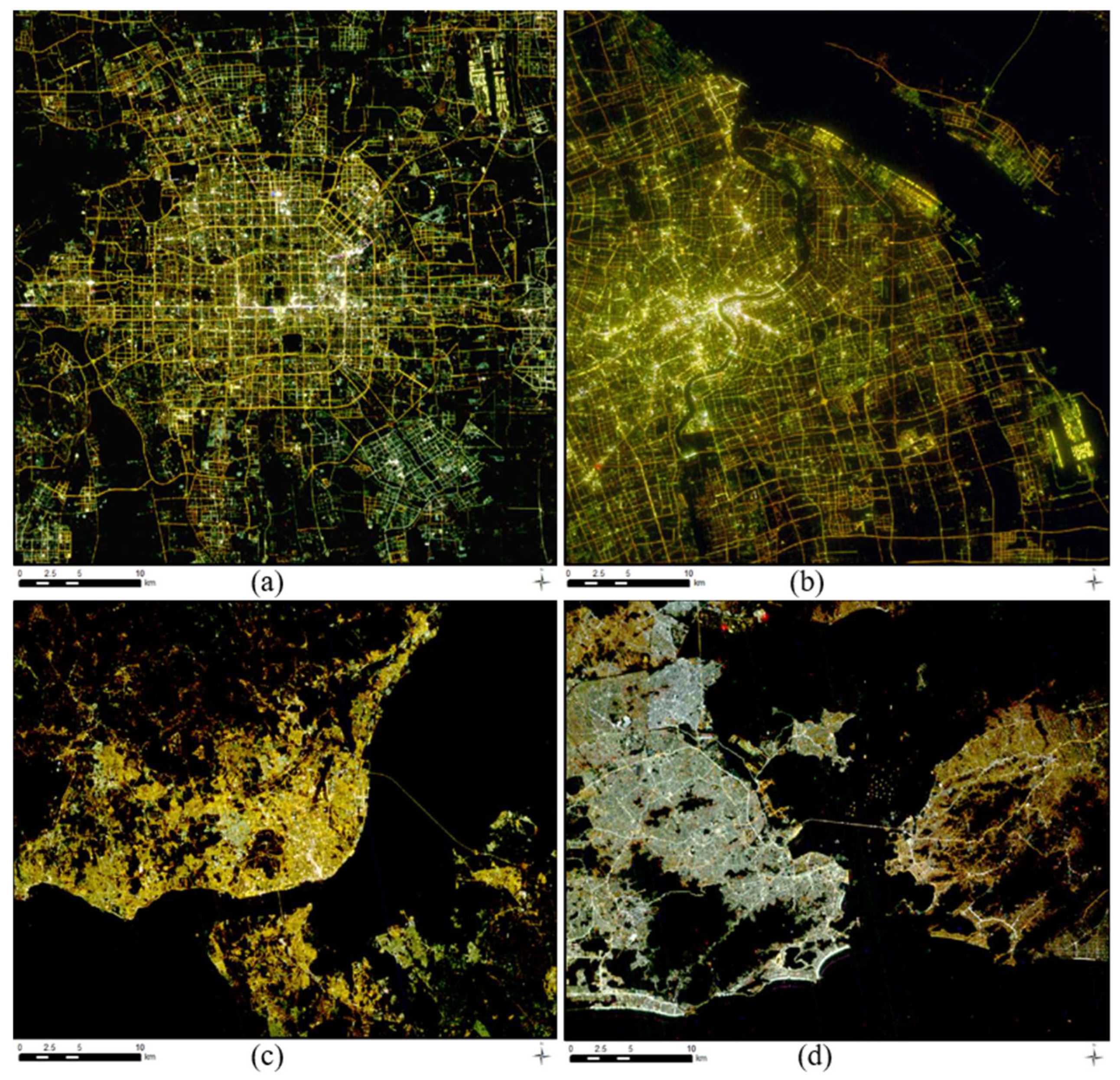
Figure 1.
The 40 m SDGSAT-1 GI color imagery of Beijing, China (a), Shanghai, China (b), Lisbon, Portugal (c), and Rio de Janeiro, Brazil (d).
Figure 1.
The 40 m SDGSAT-1 GI color imagery of Beijing, China (a), Shanghai, China (b), Lisbon, Portugal (c), and Rio de Janeiro, Brazil (d).
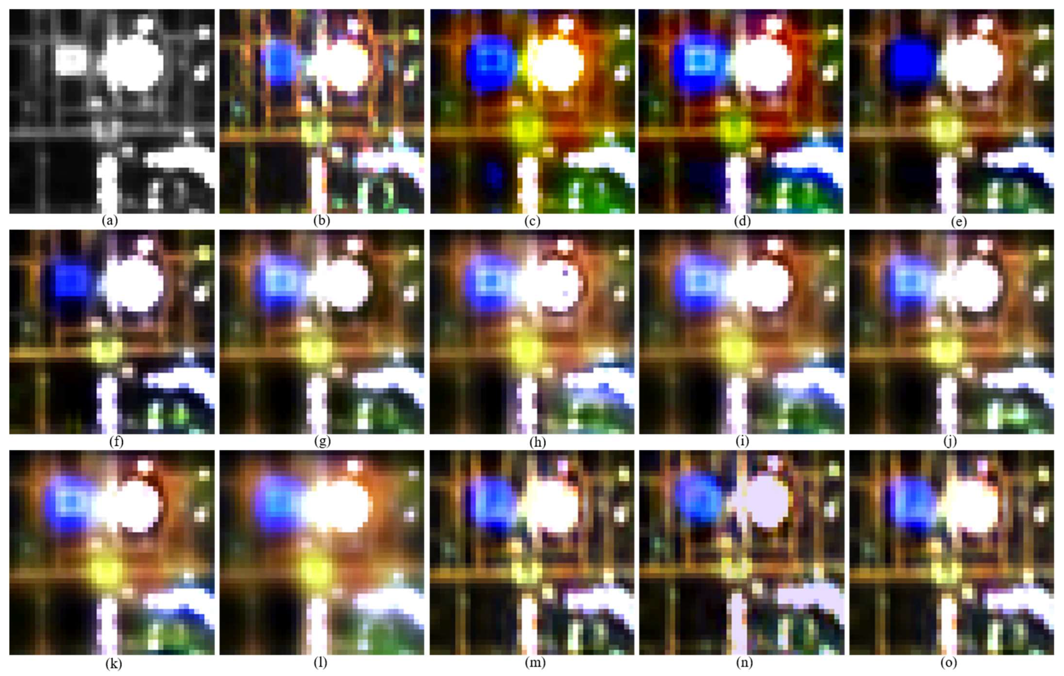
Figure 2.
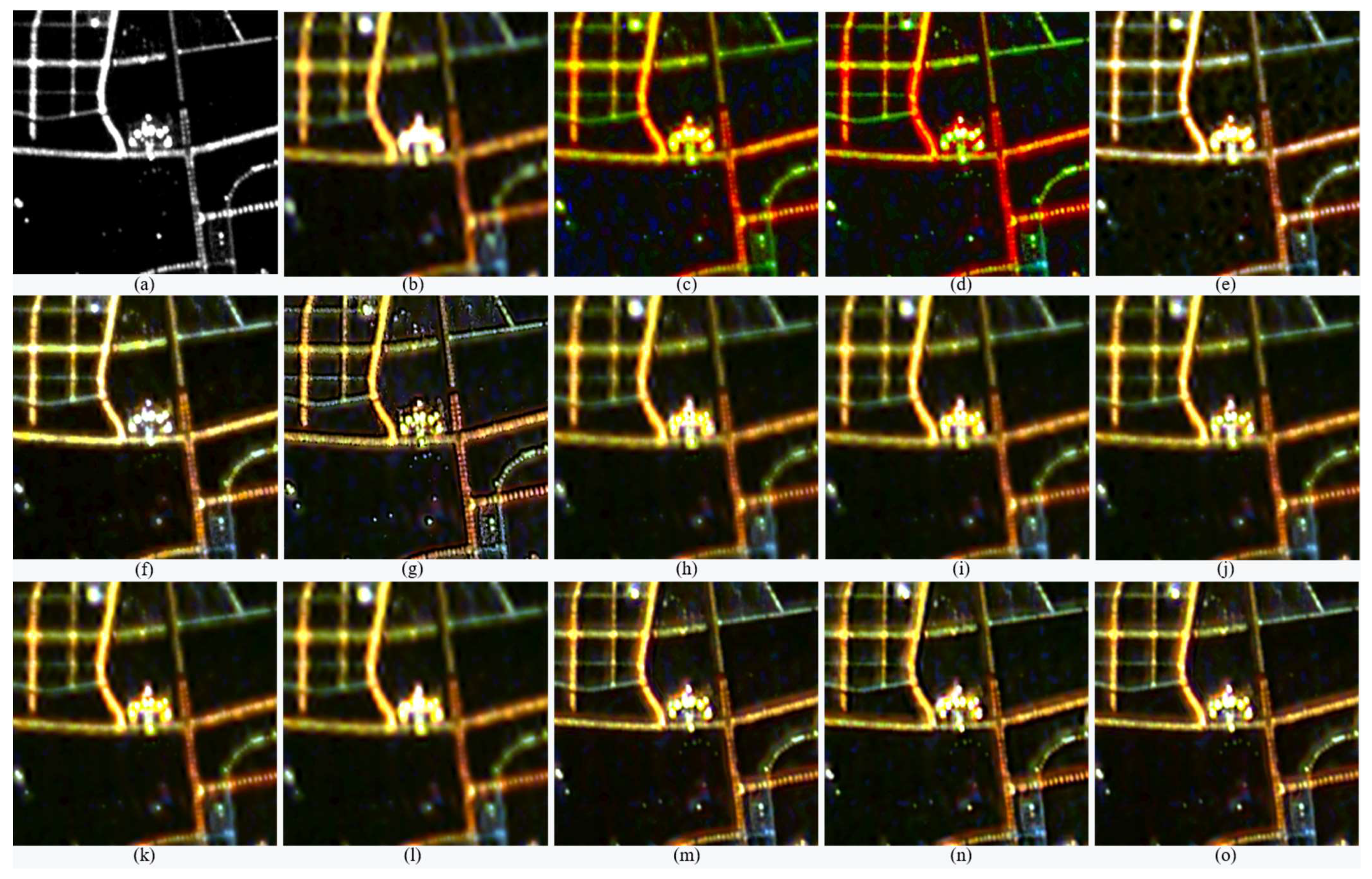
The degraded PAN, original MS images, and fused products of the degraded Beijing dataset. (a) PAN image at 40 m, (b) original MS image at 40 m, and fused products of IHS (c), PCA (d), GSA (e), RMI (f), HR (g), HPF (h), ATWT (i), GLP_HPM (j), GLP (k), GLP_CBD (l), A-PNN (m), PanNet (n), and Z-PNN (o).
Figure 2.
The degraded PAN, original MS images, and fused products of the degraded Beijing dataset. (a) PAN image at 40 m, (b) original MS image at 40 m, and fused products of IHS (c), PCA (d), GSA (e), RMI (f), HR (g), HPF (h), ATWT (i), GLP_HPM (j), GLP (k), GLP_CBD (l), A-PNN (m), PanNet (n), and Z-PNN (o).
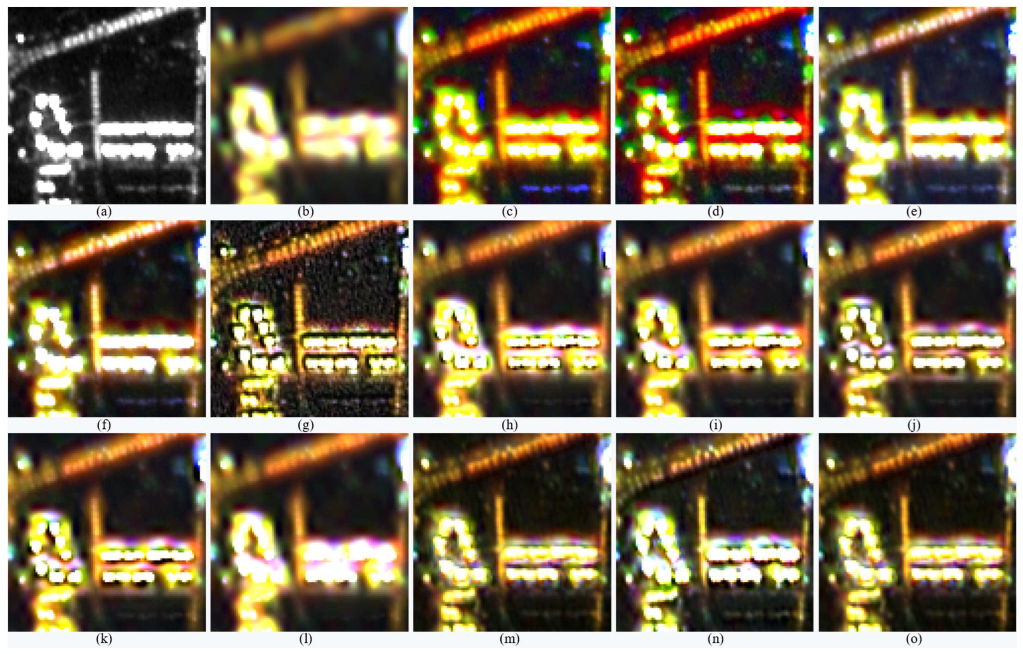
Figure 3.
The original PAN, upsampled MS images, and fused products of the original-scale Beijing dataset. (a) The PAN image of 10 m, (b) the upsampled version of the 40 m MS image, and the fused products of IHS (c), PCA (d), GSA (e), RMI (f), HR (g), HPF (h), ATWT (i), GLP_HPM (j), GLP (k), GLP_CBD (l), A-PNN (m), PanNet (n), and Z-PNN (o).
Figure 4.
The degraded PAN image, the original MS image, and fused products of the degraded Brazil dataset. (a) The PAN image of 40 m, (b) the original MS image of 40 m, and the fused products of IHS (c), PCA (d), GSA (e), RMI (f), HR (g), HPF (h), ATWT (i), GLP_HPM (j), GLP (k), GLP_CBD (l), A-PNN (m), PanNet (n), and Z-PNN (o).
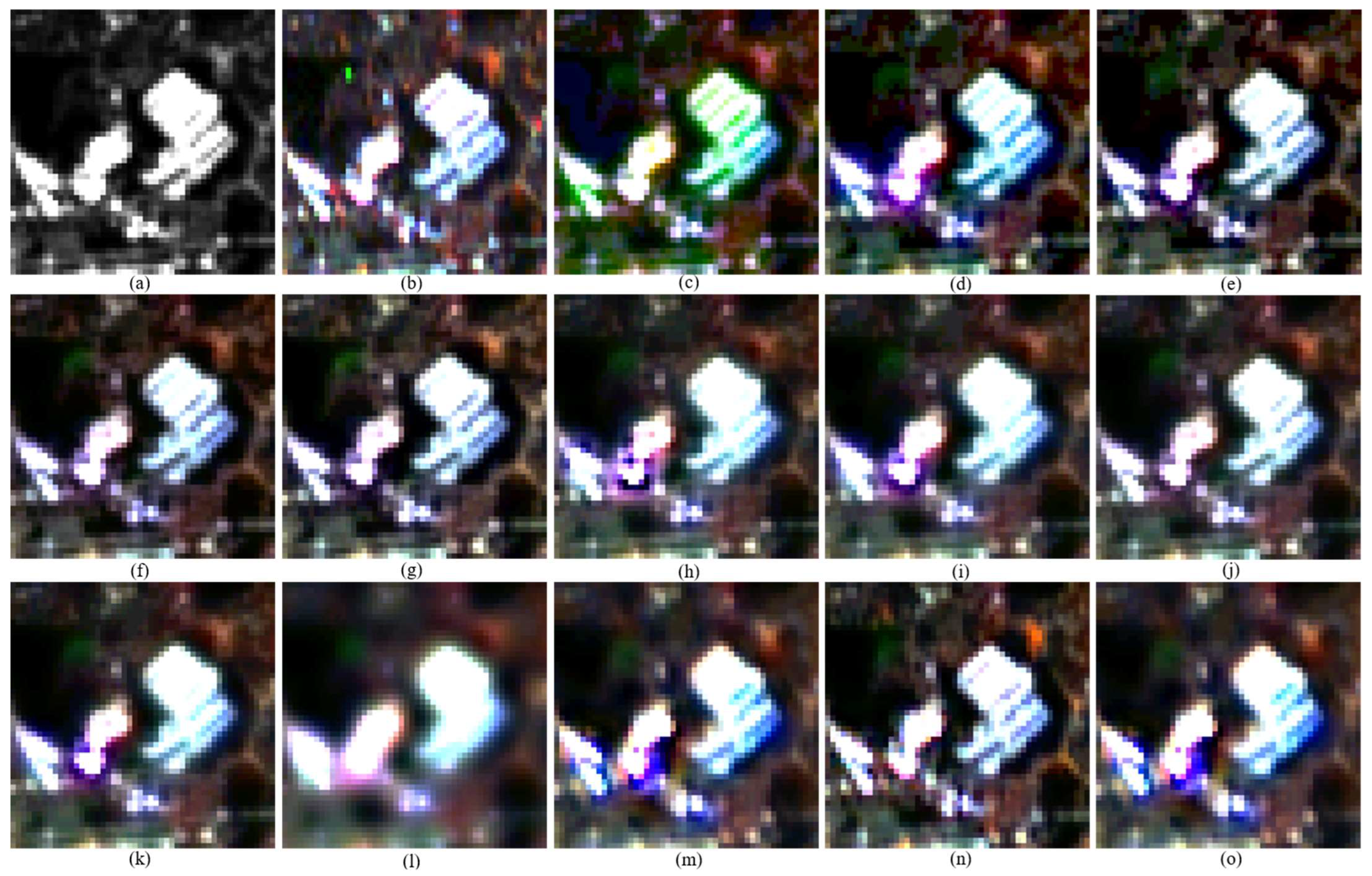
Figure 5.
The original PAN, upsampled MS images, and fused products of the original-scale Brazil dataset. (a) The PAN image of 10 m, (b) the upsampled version of the 40 m MS image, and the fused products of IHS (c), PCA (d), GSA (e), RMI (f), HR (g), HPF (h), ATWT (i), GLP_HPM (j), GLP (k), GLP_CBD (l), A-PNN (m), PanNet (n), and Z-PNN (o).
Figure 6.
The original PAN, upsampled MS images, and fused products of the original-scale Lisbon dataset. (a) The PAN image of 10 m, (b) the upsampled version of the 40 m MS image, and the fused products of IHS (c), PCA (d), GSA (e), RMI (f), HR (g), HPF (h), ATWT (i), GLP_HPM (j), GLP (k), GLP_CBD (l), A-PNN (m), PanNet (n), and Z-PNN (o).
Figure 7.
The original PAN, upsampled MS images, and fused products of the original-scale Shanghai dataset. (a) The PAN image of 10 m, (b) the upsampled version of the 40 m MS image, and the fused products of IHS (c), PCA (d), GSA (e), RMI (f), HR (g), HPF (h), ATWT (i), GLP_HPM (j), GLP (k), GLP_CBD (l), A-PNN (m), PanNet (n), and Z-PNN (o).
Table 1.
Band parameters of the GI of SDGSAT-1.
Table 1.
Band parameters of the GI of SDGSAT-1.
| Band | Center Wavelength (nm) | Wavelength Range (nm) | Bandwidth
(nm) | Spatial Resolution (m) | SNR (Observed Objects with a
Reflectance Higher than 0.2) |
|---|
| Panchromatic | 680.72 | 444–910 | 466 | 10 | Lights on city trunk roads ≥ 30;
Urban residential district ≥ 20;
Polar moon light ≥ 10. |
| Blue | 478.87 | 424–526 | 102 | 40 | Lights on city trunk roads ≥ 15;
Urban residential district ≥ 10. |
| Green | 561.20 | 506–612 | 96 | 40 |
| Red | 734.25 | 600–894 | 294 | 40 |
Table 2.
Four SDGSAT-1 NL datasets used for the evaluation of pansharpening methods.
Table 2.
Four SDGSAT-1 NL datasets used for the evaluation of pansharpening methods.
| Id | Location | Sensor | Date | Image Size (MS/PAN) |
|---|
| 1 | Beijing | SDGSAT-1 GI | November 2021 | 512 × 512/2048 × 2048 |
| 2 | Lisbon | SDGSAT-1 GI | January 2022 | 512 × 512/2048 × 2048 |
| 3 | Shanghai | SDGSAT-1 GI | April 2022 | 512 × 512/2048 × 2048 |
| 4 | Brazil | SDGSAT-1 GI | June 2022 | 512 × 512/2048 × 2048 |
Table 3.
The statistics of the four SDGSAT-1GI nighttime light datasets.
Table 3.
The statistics of the four SDGSAT-1GI nighttime light datasets.
| Dataset | Band | Minimum | Maximum | Mean | Standard Deviation |
|---|
| Beijing | R | 1 | 4426 | 412.26 | 522.81 |
| G | 1 | 4643 | 396.93 | 530.18 |
| B | 1 | 4411 | 135.11 | 315.24 |
| PAN | 1 | 4465 | 35.37 | 153.17 |
| Lisbon | R | 1 | 3852 | 270.96 | 411.55 |
| G | 1 | 4079 | 180.75 | 301.28 |
| B | 1 | 3487 | 27.69 | 89.97 |
| PAN | 1 | 4152 | 13.47 | 37.05 |
| Shanghai | R | 7 | 4357 | 236.24 | 339.20 |
| G | 7 | 4616 | 219.54 | 343.54 |
| B | 7 | 4427 | 67.80 | 176.19 |
| PAN | 7 | 4420 | 17.17 | 78.74 |
| Brazil | R | 7 | 3789 | 230.14 | 218.47 |
| G | 7 | 3935 | 300.94 | 33.92 |
| B | 7 | 3962 | 126.52 | 33.06 |
| PAN | 7 | 3620 | 19.09 | 32.89 |
Table 6.
Quality indices of fused products of the Beijing dataset at the reduced scale. The symbol ↓ denotes the lower the index value, the better the performance; ↑ means the reverse.
Table 6.
Quality indices of fused products of the Beijing dataset at the reduced scale. The symbol ↓ denotes the lower the index value, the better the performance; ↑ means the reverse.
| Method | ERGAS ↓ | SAM ↓ | UIQI ↑ | SCC ↑ | SSIM ↑ | PSNR ↑ |
|---|
| IHS | 25.749 | 11.539 | 0.582 | 0.522 | 0.658 | 24.117 |
| PCA | 23.637 | 9.625 | 0.584 | 0.528 | 0.665 | 23.910 |
| GSA | 21.987 | 9.777 | 0.819 | 0.589 | 0.870 | 25.541 |
| RMI | 19.307 | 8.532 | 0.807 | 0.624 | 0.871 | 26.208 |
| HR | 17.289 | 8.907 | 0.854 | 0.592 | 0.895 | 26.770 |
| HPF | 18.494 | 8.818 | 0.792 | 0.522 | 0.853 | 26.166 |
| ATWT | 17.550 | 8.856 | 0.812 | 0.539 | 0.869 | 26.560 |
| GLP | 17.384 | 8.876 | 0.816 | 0.543 | 0.873 | 26.599 |
| GLP_HPM | 16.360 | 8.584 | 0.846 | 0.593 | 0.890 | 27.012 |
| GLP_CBD | 17.990 | 8.785 | 0.776 | 0.522 | 0.838 | 26.100 |
| A-PNN | 12.159 | 8.803 | 0.930 | 0.784 | 0.964 | 30.813 |
| PanNet | 9.287 | 8.199 | 0.952 | 0.864 | 0.974 | 33.029 |
| Z-PNN | 17.312 | 9.886 | 0.866 | 0.629 | 0.919 | 27.191 |
| EXP | 25.309 | 8.535 | 0.609 | 0.205 | 0.751 | 23.530 |
Table 7.
Quality indices of fused products of the Beijing dataset at the original scale. The symbol ↓ denotes the lower the index value, the better the performance; ↑ means the reverse.
Table 7.
Quality indices of fused products of the Beijing dataset at the original scale. The symbol ↓ denotes the lower the index value, the better the performance; ↑ means the reverse.
| Method | ↓ | ↓ | QNR ↑ | ↓ | HQNR ↑ | ↓ |
|---|
| IHS | 0.465 | 0.017 | 0.526 | 0.417 | 0.573 | 0.254 |
| PCA | 0.351 | 0.019 | 0.636 | 0.456 | 0.533 | 0.228 |
| GSA | 0.035 | 0.012 | 0.953 | 0.215 | 0.775 | 0.141 |
| RMI | 0.011 | 0.016 | 0.973 | 0.223 | 0.765 | 0.158 |
| HR | 0.211 | 0.003 | 0.787 | 0.239 | 0.759 | 0.149 |
| HPF | 0.025 | 0.009 | 0.966 | 0.027 | 0.964 | 0.296 |
| ATWT | 0.035 | 0.009 | 0.956 | 0.029 | 0.962 | 0.275 |
| GLP | 0.035 | 0.009 | 0.956 | 0.033 | 0.958 | 0.270 |
| GLP_HPM | 0.031 | 0.010 | 0.959 | 0.033 | 0.957 | 0.285 |
| GLP_CBD | 0.020 | 0.008 | 0.972 | 0.024 | 0.968 | 0.440 |
| A-PNN | 0.109 | 0.082 | 0.817 | 0.491 | 0.467 | 0.365 |
| PanNet | 0.097 | 0.087 | 0.825 | 0.490 | 0.465 | 0.271 |
| Z-PNN | 0.081 | 0.088 | 0.838 | 0.441 | 0.509 | 0.094 |
Table 8.
Quality indices of fused products of the Brazil dataset at the reduced scale. The symbol ↓ denotes the lower the index value, the better the performance; ↑ means the reverse.
Table 8.
Quality indices of fused products of the Brazil dataset at the reduced scale. The symbol ↓ denotes the lower the index value, the better the performance; ↑ means the reverse.
| Method | ERGAS ↓ | SAM ↓ | UIQI ↑ | SCC ↑ | SSIM ↑ | PSNR ↑ |
|---|
| IHS | 15.120 | 11.002 | 0.646 | 0.557 | 0.780 | 29.163 |
| PCA | 14.034 | 9.333 | 0.666 | 0.586 | 0.795 | 29.259 |
| GSA | 14.044 | 9.877 | 0.774 | 0.597 | 0.876 | 29.615 |
| RMI | 15.120 | 11.002 | 0.646 | 0.557 | 0.780 | 29.163 |
| HR | 11.196 | 8.952 | 0.797 | 0.589 | 0.917 | 31.294 |
| HPF | 11.305 | 8.943 | 0.794 | 0.587 | 0.914 | 31.210 |
| ATWT | 10.318 | 8.741 | 0.821 | 0.633 | 0.928 | 31.901 |
| GLP | 13.894 | 8.865 | 0.671 | 0.516 | 0.849 | 28.655 |
| GLP_HPM | 11.779 | 8.690 | 0.790 | 0.593 | 0.906 | 30.853 |
| GLP_CBD | 16.009 | 8.690 | 0.579 | 0.182 | 0.682 | 22.255 |
| A-PNN | 17.151 | 18.711 | 0.701 | 0.493 | 0.802 | 29.214 |
| PanNet | 6.134 | 8.410 | 0.928 | 0.866 | 0.976 | 36.884 |
| Z-PNN | 11.780 | 9.766 | 0.786 | 0.583 | 0.907 | 11.780 |
| EXP | 14.034 | 9.333 | 0.666 | 0.586 | 0.795 | 29.259 |
Table 9.
Quality indexes of fused products of the Brazil dataset at the original scale. The symbol ↓ denotes the lower the index value, the better the performance; ↑ means the reverse.
Table 9.
Quality indexes of fused products of the Brazil dataset at the original scale. The symbol ↓ denotes the lower the index value, the better the performance; ↑ means the reverse.
| Method | ↓ | ↓ | QNR ↑ | ↓ | HQNR ↑ | ↓ |
|---|
| IHS | 0.093 | 0.008 | 0.900 | 0.466 | 0.530 | 0.288 |
| PCA | 0.066 | 0.010 | 0.924 | 0.449 | 0.546 | 0.277 |
| GSA | 0.097 | 0.003 | 0.901 | 0.377 | 0.621 | 0.257 |
| RMI | 0.083 | 0.005 | 0.912 | 0.322 | 0.675 | 0.271 |
| HR | 0.212 | 0.001 | 0.787 | 0.261 | 0.738 | 0.391 |
| HPF | 0.054 | 0.006 | 0.941 | 0.042 | 0.952 | 0.363 |
| ATWT | 0.067 | 0.006 | 0.928 | 0.048 | 0.946 | 0.332 |
| GLP | 0.069 | 0.006 | 0.926 | 0.048 | 0.946 | 0.331 |
| GLP_HPM | 0.061 | 0.006 | 0.933 | 0.047 | 0.948 | 0.325 |
| GLP_CBD | 0.013 | 0.004 | 0.983 | 0.039 | 0.957 | 0.598 |
| A-PNN | 0.008 | 0.014 | 0.978 | 0.481 | 0.512 | 0.479 |
| PanNet | 0.051 | 0.029 | 0.921 | 0.555 | 0.432 | 0.443 |
| Z-PNN | 0.040 | 0.035 | 0.926 | 0.496 | 0.487 | 0.312 |
Table 10.
Quality indices of fused products of the Lisbon dataset at the reduced scale. The symbol ↓ denotes the lower the index value, the better the performance; ↑ means the reverse.
Table 10.
Quality indices of fused products of the Lisbon dataset at the reduced scale. The symbol ↓ denotes the lower the index value, the better the performance; ↑ means the reverse.
| Method | ERGAS ↓ | SAM ↓ | UIQI ↑ | SCC ↑ | SSIM ↑ | PSNR ↑ |
|---|
| IHS | 37.421 | 13.805 | 0.619 | 0.694 | 0.735 | 29.684 |
| PCA | 28.072 | 15.258 | 0.653 | 0.756 | 0.796 | 29.666 |
| GSA | 24.244 | 15.455 | 0.839 | 0.781 | 0.967 | 33.083 |
| RMI | 24.502 | 13.717 | 0.770 | 0.777 | 0.946 | 32.594 |
| HR | 20.541 | 14.247 | 0.848 | 0.779 | 0.964 | 33.260 |
| HPF | 25.456 | 14.117 | 0.807 | 0.738 | 0.945 | 31.841 |
| ATWT | 24.749 | 14.312 | 0.823 | 0.751 | 0.956 | 32.459 |
| GLP | 24.403 | 14.033 | 0.827 | 0.752 | 0.959 | 32.633 |
| GLP_HPM | 19.011 | 13.829 | 0.862 | 0.799 | 0.971 | 34.197 |
| GLP_CBD | 26.766 | 13.803 | 0.712 | 0.594 | 0.882 | 28.706 |
| A-PNN | 18.777 | 14.531 | 0.880 | 0.823 | 0.982 | 35.663 |
| PanNet | 14.219 | 12.492 | 0.907 | 0.888 | 0.987 | 37.185 |
| Z-PNN | 25.077 | 16.884 | 0.781 | 0.721 | 0.943 | 32.384 |
| EXP | 34.892 | 13.717 | 0.601 | 0.194 | 0.839 | 26.317 |
Table 11.
Quality indices of fused products of the Lisbon dataset at the original scale. The symbol ↓ denotes the lower the index value, the better the performance; ↑ means the reverse.
Table 11.
Quality indices of fused products of the Lisbon dataset at the original scale. The symbol ↓ denotes the lower the index value, the better the performance; ↑ means the reverse.
| Method | ↓ | ↓ | QNR ↑ | ↓ | HQNR ↑ | ↓ |
|---|
| IHS | 0.066 | 0.006 | 0.929 | 0.612 | 0.385 | 0.168 |
| PCA | 0.036 | 0.003 | 0.961 | 0.486 | 0.512 | 0.154 |
| GSA | 0.092 | 0.004 | 0.904 | 0.342 | 0.656 | 0.106 |
| RMI | 0.073 | 0.004 | 0.923 | 0.385 | 0.612 | 0.166 |
| HR | 0.433 | 0.003 | 0.565 | 0.451 | 0.547 | 0.153 |
| HPF | 0.079 | 0.005 | 0.916 | 0.097 | 0.899 | 0.180 |
| ATWT | 0.088 | 0.005 | 0.908 | 0.111 | 0.885 | 0.156 |
| GLP | 0.088 | 0.004 | 0.908 | 0.150 | 0.846 | 0.155 |
| GLP_HPM | 0.081 | 0.004 | 0.915 | 0.146 | 0.850 | 0.160 |
| GLP_CBD | 0.011 | 0.003 | 0.985 | 0.063 | 0.934 | 0.565 |
| A-PNN | 0.057 | 0.114 | 0.836 | 0.792 | 0.185 | 0.498 |
| PanNet | 0.061 | 0.115 | 0.830 | 0.793 | 0.183 | 0.416 |
| Z-PNN | 0.069 | 0.218 | 0.728 | 0.780 | 0.172 | 0.192 |
Table 12.
Quality indices of fused products of the Shanghai dataset at the reduced scale. The symbol ↓ denotes the lower the index value, the better the performance; ↑ means the reverse.
Table 12.
Quality indices of fused products of the Shanghai dataset at the reduced scale. The symbol ↓ denotes the lower the index value, the better the performance; ↑ means the reverse.
| Method | ERGAS ↓ | SAM ↓ | UIQI ↑ | SCC ↑ | SSIM ↑ | PSNR ↑ |
|---|
| IHS | 31.057 | 13.215 | 0.450 | 0.574 | 0.709 | 27.916 |
| PCA | 28.578 | 10.710 | 0.452 | 0.595 | 0.721 | 27.690 |
| GSA | 22.660 | 10.901 | 0.785 | 0.675 | 0.912 | 30.767 |
| RMI | 21.720 | 9.306 | 0.792 | 0.725 | 0.927 | 31.132 |
| HR | 19.713 | 10.026 | 0.870 | 0.783 | 0.954 | 31.103 |
| HPF | 22.560 | 9.535 | 0.747 | 0.578 | 0.901 | 29.942 |
| ATWT | 21.205 | 9.565 | 0.764 | 0.600 | 0.910 | 30.409 |
| GLP | 20.800 | 9.582 | 0.769 | 0.604 | 0.914 | 30.507 |
| GLP_HPM | 17.409 | 9.388 | 0.816 | 0.688 | 0.935 | 31.881 |
| GLP_CBD | 22.593 | 9.519 | 0.714 | 0.548 | 0.884 | 29.356 |
| A-PNN | 13.787 | 9.126 | 0.903 | 0.825 | 0.893 | 35.811 |
| PanNet | 10.194 | 8.572 | 0.924 | 0.900 | 0.907 | 38.363 |
| Z-PNN | 19.206 | 11.432 | 0.818 | 0.702 | 0.808 | 32.077 |
| EXP | 31.666 | 9.306 | 0.577 | 0.209 | 0.833 | 27.460 |
Table 13.
Quality indices of fused products of the Shanghai dataset at the original scale. The symbol ↓ denotes the lower the index value, the better the performance; ↑ means the reverse.
Table 13.
Quality indices of fused products of the Shanghai dataset at the original scale. The symbol ↓ denotes the lower the index value, the better the performance; ↑ means the reverse.
| Method | ↓ | ↓ | QNR ↑ | ↓ | HQNR ↑ | ↓ |
|---|
| IHS | 0.551 | 0.010 | 0.444 | 0.442 | 0.552 | 0.618 |
| PCA | 0.430 | 0.011 | 0.563 | 0.491 | 0.504 | 0.606 |
| GSA | 0.053 | 0.006 | 0.941 | 0.291 | 0.704 | 0.561 |
| RMI | 0.041 | 0.008 | 0.952 | 0.260 | 0.735 | 0.571 |
| HR | 0.226 | 0.002 | 0.772 | 0.229 | 0.769 | 0.560 |
| HPF | 0.017 | 0.004 | 0.979 | 0.032 | 0.964 | 0.635 |
| ATWT | 0.025 | 0.004 | 0.971 | 0.031 | 0.965 | 0.625 |
| GLP | 0.024 | 0.004 | 0.971 | 0.033 | 0.963 | 0.621 |
| GLP_HPM | 0.023 | 0.004 | 0.973 | 0.033 | 0.963 | 0.615 |
| GLP_CBD | 0.014 | 0.004 | 0.983 | 0.032 | 0.964 | 0.714 |
| A-PNN | 0.095 | 0.053 | 0.857 | 0.677 | 0.306 | 0.638 |
| PanNet | 0.083 | 0.049 | 0.872 | 0.681 | 0.303 | 0.594 |
| Z-PNN | 0.111 | 0.075 | 0.822 | 0.677 | 0.299 | 0.439 |


