Abstract
Dissolved oxygen (DO) is essential for assessing and monitoring the health of marine ecosystems. The phenomenon of ocean deoxygenation is widely recognized. Nevertheless, the limited availability of observations poses a challenge in achieving a comprehensive understanding of global ocean DO dynamics and trends. The study addresses the challenge of unevenly distributed Argo DO data by developing time–space–depth machine learning (TSD-ML), a novel machine learning-based model designed to enhance reconstruction accuracy in data-sparse regions. TSD-ML partitions Argo data into segments based on time, depth, and spatial dimensions, and conducts model training for each segment. This research contrasts the effectiveness of partitioned and non-partitioned modeling approaches using three distinct ML regression methods. The results reveal that TSD-ML significantly enhances reconstruction accuracy in areas with uneven DO data distribution, achieving a 30% reduction in root mean square error (RMSE) and a 20% decrease in mean absolute error (MAE). In addition, a comparison with WOA18 and GLODAPv2 ship survey data confirms the high accuracy of the reconstructions. Analysis of the reconstructed global ocean DO trends over the past two decades indicates an alarming expansion of anoxic zones.
1. Introduction
Dissolved oxygen (DO) pertains to the quantity of free and non-compound oxygen that has dissolved within water [1]. DO primarily originates from the atmosphere and photosynthesis, while being influenced by ocean currents, biological activities, and environmental factors such as sea level pressure (SLP), seawater temperature, and salinity [2,3], which significantly support essential processes such as respiration, metabolism, and biodiversity within marine ecosystems [4,5,6,7]. Understanding and monitoring the dynamics of DO is essential for effective conservation and management of our oceans, providing valuable insights into water quality and the ecological status of marine environments.
Ocean deoxygenation has become common knowledge and has gained increased attention worldwide in recent years [8,9,10,11,12]. The findings derived from the 6th Coupled Model Intercomparison Project (CMIP6) [13] project a diminution in the global oceanic oxygen content by approximately 3 to 4% by the conclusion of the 21st century [14]. This projection is corroborated by a synthesis of observational data, which indicates a loss of approximately 1 to 2% of the global oxygen inventory since the mid-20th century [15,16]. Comprehensive research on ocean DO needs substantial data. However, due to the lack of data, the status of global ocean DO is still unclear. The World Ocean Atlas 2018 (WOA18) provides quality-controlled DO data, but is limited to climatological monthly resolutions [17]. The Global Ocean Data Analysis Project version 2 (GLODAPv2) primarily relies on ship-based measurements for its DO data, with the majority of its profiling trajectories aligning closely with the routes of maritime voyages. Unfortunately, data at a monthly scale remains notably scarce [18,19,20]. In recent years, satellite observations have been used to assess DO trends over longer periods of time [21]. Nevertheless, these satellite observations lack the ability to apprehend fluctuations in DO beneath the water’s surface. The proliferation in situ DO measurements at various depths has witnessed a substantial rise due to the advancement of autonomous oceanic observation systems, notably the biogeochemical Argo (BGC-Argo) floats [22].
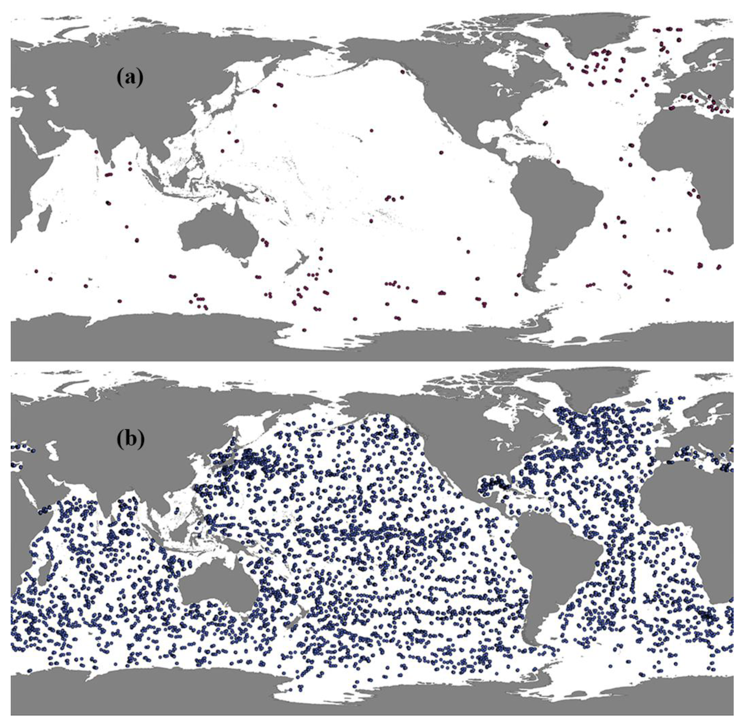
Core-Argo constitutes the central component of the Argo Program, a project initiated in the year 2000, primarily dedicated to measuring and mapping the distribution of temperature and salinity in the oceans. From 1999 to 2022, over 150,000 Core-Argo floats were deployed in oceans globally. BGC-Argo floats are equipped with sensors mainly to observe marine optical parameters [23], e.g., DO, chlorophyll a, etc. Although the emergence of BGC-Argo floats dates back to 2002, it was not until the formal initiation of the BGC-Argo project in 2016 that a more systematic and widespread deployment began. Despite this, until today the distribution of these floats remains highly uneven, with a notably higher density in regions such as the Southern Ocean. The limited number of BGC-Argo floats results in inadequate observational data, constraining our ability to analyze the global spatiotemporal dynamics of DO (Figure 1).
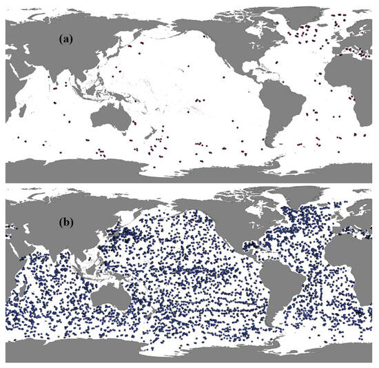
Figure 1.
(a) Dissolved oxygen (DO) spatial distribution at a depth layer of 200 dbar by BGC-Argo floats in January 2020 and (b) temperature and salinity spatial distribution at the same depth by Core-Argo floats in January 2020.
Currently, various models have been developed to estimate DO, including traditional methods and ML methods. Traditionally, methods utilizing low-order oceanic biogeochemical models and climate system models have been employed to estimate DO [24,25]. Mathematical modeling is another commonly used method to estimate DO [26]. With the development of observational techniques and the increase in oceanic data, ML methods have demonstrated advantages over traditional methods, including faster computational speed, better robustness [27], fewer assumptions about the data, and the ability to model highly nonlinear relationships between the variables and effectively estimate target variable from sparse observations [28,29]. Some ML methods have been employed to analyze ocean DO data. Giglio, et al. [30] used the random forest regression (RF) algorithm to estimate DO in the Southern Ocean based on Argo profiles, demonstrating that the RF algorithm is a valuable tool for multivariate mapping. Sharp, et al. [31] inverted the global ocean oxygen field using Argo and GLODAPv2 data based on RF and feed-forward neural network approaches. In addition, deep learning methods have also been used for DO prediction [32].
Current DO estimation methods are not yet suitable for using Argo data for global ocean DO reconstruction. Limitations are as follows: (1) Some methods rely on satellite products with wide spatial coverage. The inversion of DO is highly constrained due to the non-optical nature of DO [33,34], especially in the deep layer; as a result most of the proposed inversion models currently perform well only in local surface areas [21] and pose challenges for generalization and broad application [35]. (2) Some studies have inverted subsurface DO using monitoring stations data [36,37] or shipboard observation data, but their scope is limited to specific types of water bodies [38,39]. Most studies estimating ocean DO have similar limitations [40], lacking global scale and long-time series coverage. (3) The distribution of DO data observed by BGC-Argo floats is sparse and uneven on a global scale. Existing studies on DO estimation using Argo data have failed to take this limitation into account [30]. Differing from the method of Sharp, Fassbender, Carter, Johnson, Schultz, and Dunne [31], this paper aims to design a modeling approach to improve the accuracy of the machine learning (ML) method in inverting data sparse regions when modeling training data with uneven spatial distribution. Therefore, when using Argo data for global ocean DO reconstruction, it is crucial to construct a model that considers the distribution characteristics of Argo data. Otherwise, directly performing reconstruction on multiple depth layers at global scale may negatively affect the performance of the model.
This study aims to develop an ML-based approach for reconstructing ocean DO. The method focuses on enhancing accuracy in regions with sparse data by employing a time–space–depth partitioning strategy, thereby effectively overcoming the challenges posed by uneven data distribution in the training model. This study uses the Argo observation data as the sole training dataset, which ensures data accuracy, as it is a homogeneous dataset with strict sampling methods and data quality control procedures. This method considers the spatial heterogeneity of DO in the global ocean during the reconstruction process and realizes the DO reconstruction of various depth layers in long-term global-scale time series by training multiple submodels. This method has good application value for making up for the global ocean DO data and provides method support for further revealing DO dynamic changes.
The remainder of the paper is organized as follows: Section 2 describes the data, models, and methods. Section 3 presents the results and discussion, including the advantage of spatial partition, an assessment of model performance, a sensitivity analysis and comparison with existing ship survey data and global DO trends. Section 4 summarizes the key findings and conclusions of the study.
2. Materials and Methods
2.1. Argo Data
The profile data from Argo floats are sourced from the Argo Data Management Center. These data are freely provided by the International Argo Program after undergoing real-time and delayed-mode quality control (website: http://argo.jcommops.org, accessed on 1 May 2023).
As of early 2023, the emerging BGC-Argo project has obtained over 260,000 DO profiles and continues steady growth at approximately 20,000 new profiles annually. From 2008 to 2022, a total of 211,397 profiles for each variable (i.e., pressure, DO, temperature, and salinity) were gathered from all BGC-Argo floats. The Core-Argo program is primarily designed for observing ocean temperature and salinity. Approximately 15,000 Core-Argo floats have been deployed in the global ocean for the period from 2005 to 2022, enabling the observation of over 2,300,000 original temperature and salinity profiles.
In this manuscript, the acquired Argo profiles are divided into three parts. The first dataset, referred to as the training dataset, is utilized for model training and validation. It consists of pressure, temperature, salinity, DO, and their corresponding temporal and spatial attributes. The second dataset, referred to as the spatial partitioning dataset, is used to spatially partition the global ocean. It includes pressure, DO, and their corresponding temporal and spatial attributes. The above two datasets are both from BGC-Argo floats observations during 2008–2022. The third dataset, known as the reconstruction dataset, is used for DO reconstruction. It comprises pressure, temperature, salinity, and their corresponding temporal and spatial attributes, which are obtained from Core-Argo floats during 2005–2022.
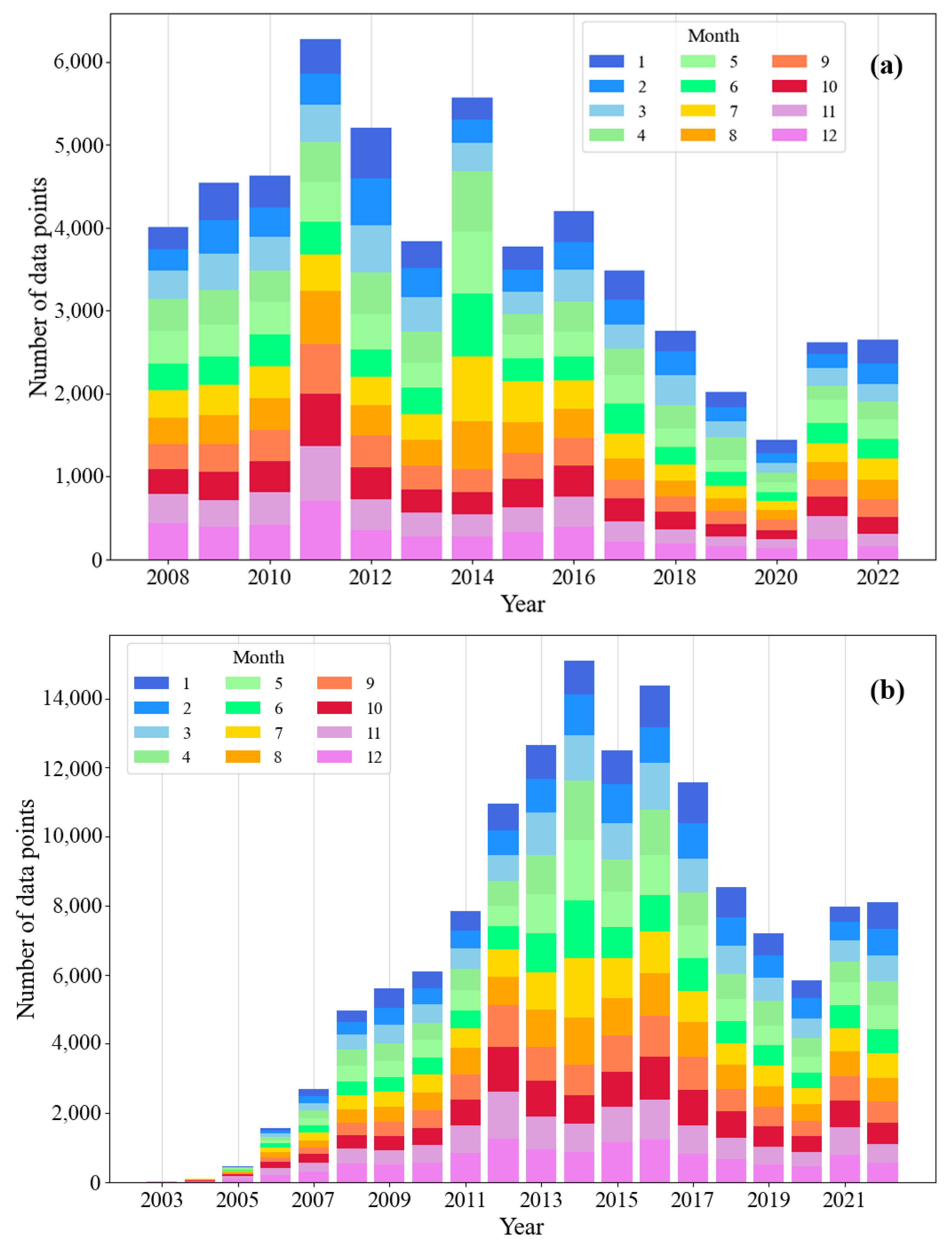
To minimize the impact of anomalous data on the model, the data used needs to undergo several screening criteria, as follows: (1) Only data points with data quality identifiers of 1 or 2 for all variables in each profile are retained; (2) Anomalous data points that were located either on land or below the seafloor are removed; (3) Anomalous data points with temperature values above 40 °C or below −5 °C are deleted; (4) Data points with salinity and DO not greater than 0 are excluded; (5) Only samples with valid values for each variable contained in each sample data are retained. The number of samples in the sample database after quality control by year and month is shown in Figure 2. Figure 2a depicts the sample counts for the training dataset and (b) is the spatially partitioned dataset sample size.

Figure 2.
Number of available Argo profiles after quality control, and the different colors means different months at a depth layer of 10 dbar. (a) is the effective training dataset sample size and (b) is the spatially partitioned dataset sample size.
2.2. Model Training
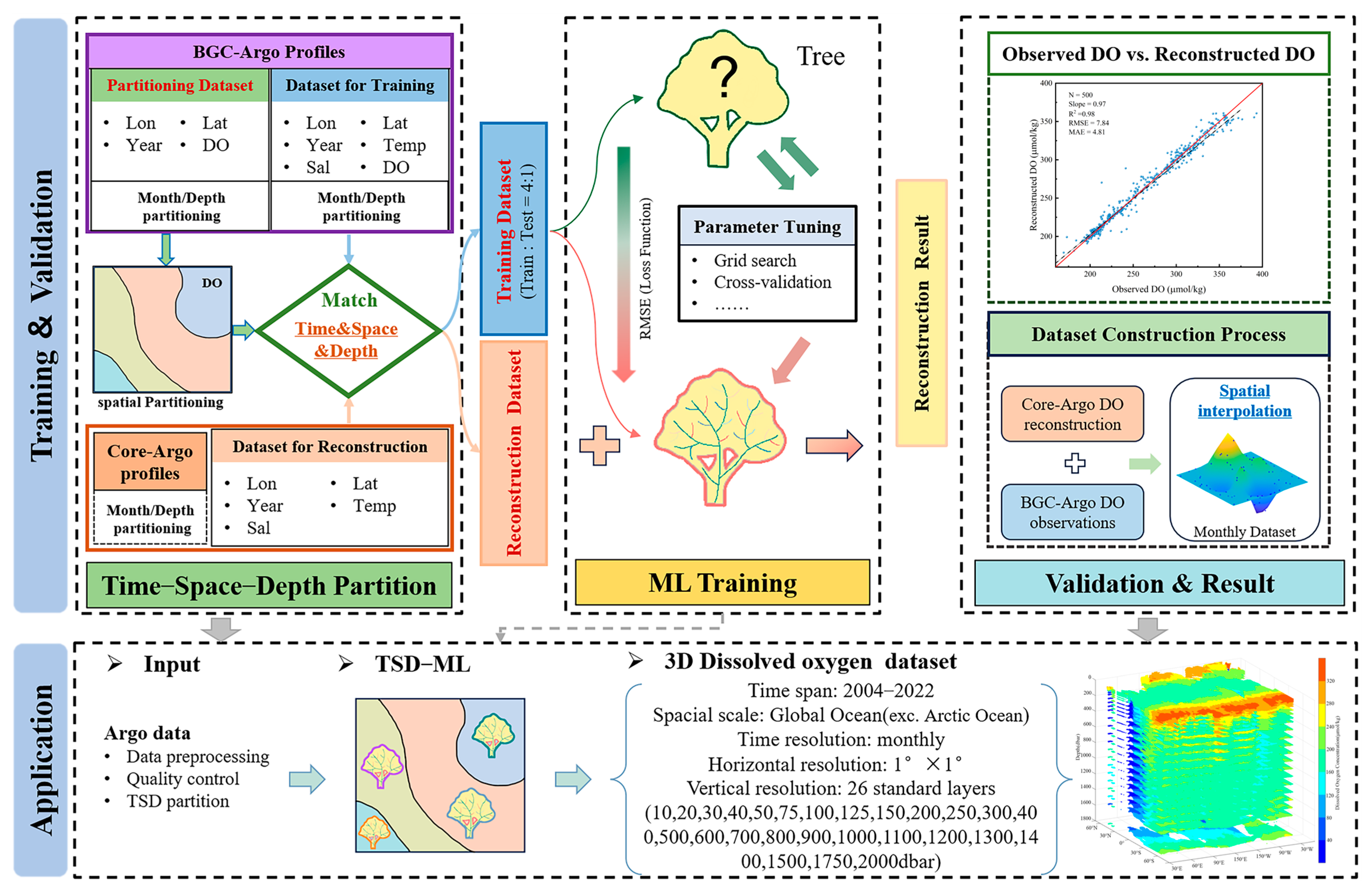
In this study, we introduce a novel approach named time–space–depth machine learning (TSD-ML). This method, as illustrated in Figure 3, incorporates the concept of time–space–depth partitioning. TSD-ML is specifically designed to enhance the reconstruction accuracy of ML regression models in areas where data is scarce. The core components of this method are the time–space–depth partitioning, coupled with model training and validation phases.
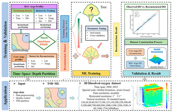
Figure 3.
Overview of time–space–depth machine learning (TSD-ML) method for reconstructing DO using Argo data.
2.2.1. Time–Space–Depth Partition
Geospatial data exhibit significant spatiotemporal correlations. It is essential to emphasize the temporal and spatial geographic characteristics of the data. The use of time–space–depth partitioning for modeling allows for better capture of spatiotemporal patterns and variability, thereby improving model accuracy. Consequently, partitioning these variables along temporal, spatial, and depth dimensions enhances the investigation of their attributes.
To specifically analyze seasonal patterns of DO, the datasets were partitioned into twelve different months, each containing several continuous time periods (e.g., January 1–31 across all years). To understand the vertical distribution and variability of DO across depth layers, the upper 2000 m of the global ocean was partitioned into 26 standard layers (10, 20, 30, 40, 50, 75, 100, 125, 150, 200, 250, 300, 400, 500, 600, 700, 800, 900, 1000, 1100, 1200, 1300, 1400, 1500, 1750, 2000 dbar), with more layers in the variable upper ocean [41]. When partitioning a particular depth layer, the first step is to select observed data within a ±5 m depth range centered on the specified depth based on pressure values. It is important to note, however, that for layers above 100 dbar, this range is refined to ±3 m to account for more pronounced environmental variability at shallower depths. Next, outlier detection using three times the standard deviation removes anomalous values from the selected data. The measured values of the input variables (temperature, salinity, and DO) are then averaged to represent the values for that depth layer.
DO data from Argo floats exhibit sparsity and heterogeneity, with dense coverage of the Southern Ocean but sparse coverage of the central Pacific. To account for the heterogeneous DO distribution, the global ocean was spatially partitioned. This provided valuable prior knowledge for model construction, while addressing the challenges of uneven data distribution, which degrades model generalization and accuracy. The partitioning dataset derived from BGC-Argo floats, unlike the training dataset, captured only all available DO measurements. The use of this dataset improved partitioning accuracy and DO data utilization during modeling. The spatial partitioning approach took into account the global heterogeneity of the DO distribution and the data distribution characteristics. The steps to spatially partition the global ocean (Figure 4) are as follows:
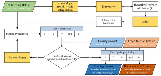
Figure 4.
Flowchart of spatial partitioning approach.
- (1)
- To generate continuous, smooth DO surfaces while accounting for seafloor topography effects, spline with barriers (SWP) interpolation was applied. This interpolated the partitioned DO data from the spatial dataset into global ocean grids (85.5°S–69.5°N, 180°E–180°W) for each depth layer and month. The spline with barriers interpolation method uses the two-dimensional minimum curvature spline technique to interpolate points to a grid surface. A negative value check is also performed on the interpolated grid to ensure that all grid cell values in the final grid are greater than zero.
- (2)
- K-means++ clustering is used to classify the interpolated climatology monthly DO grids. The K-means++ algorithm is an optimization of the K-means method of randomly initializing the centroid and can select a better cluster center in the cluster center selection process. After testing various scenarios, the number of clustering clusters (k) selected in this article ranges from 2 to 12, with clustering performed sequentially for each k value. The corresponding sum of squared error (SSE) was computed to evaluate the clustering effectiveness by summing the squared distances between data points and cluster centers. SSE values were obtained for different k. The optimal k was determined using the elbow method. As k increases, the SSE decreases, but slows down after an elbow point.
- (3)
- The optimal number of clusters was entered into the Jenks natural breaks classification method to categorize the interpolated monthly DO data by minimizing intraclass differences and maximizing interclass differences, while paying more attention to the spatial correlation of partition breakpoints. Excessive data ranges for some partitions are avoided, helping to improve interpretability of results and analytical applications.
- (4)
- Partition labels were assigned to the training data based on location and month. Some partitions had insufficient samples for training, so partitions below the sample threshold (T = 300) were merged. The principle of merging is to merge only spatially adjacent partitions and to ensure the maximum number of partitions. The merging rules were as follows: (a) the partitions above the sample threshold are added directly to the subset; (b) if below the threshold, it is merged with the neighboring partition with fewer samples until the condition is met; and (c) each partition name appears only once in all subsets. These rules ensure sufficient samples for model training while maximizing spatial heterogeneity considerations.
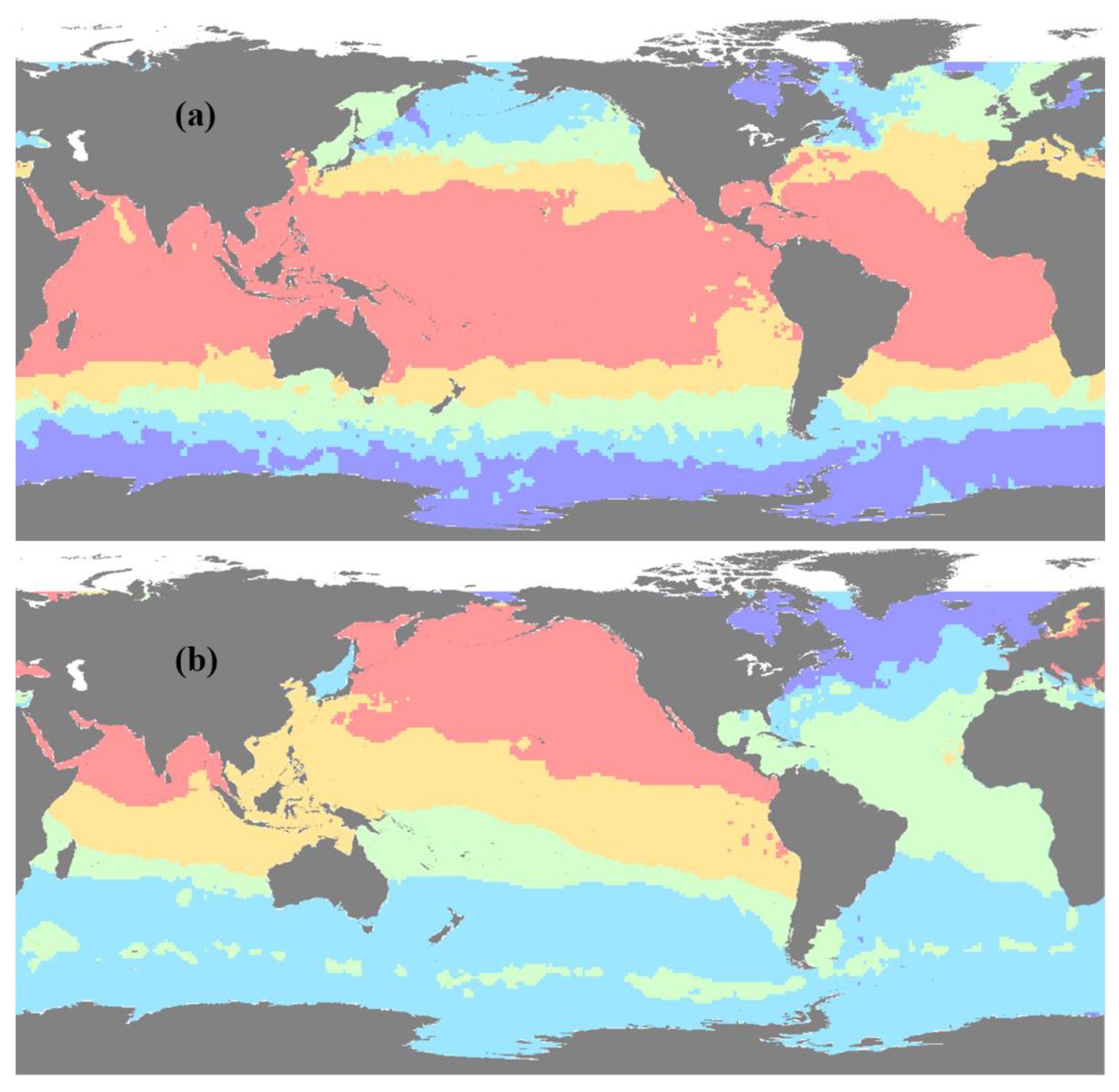
Figure 5 displays the spatial partitioning results for January at 10 dbar and 1000 dbar, where different colors represent distinct partitions. In both depth layers, the global ocean is divided into five partitions. Finally, the training and reconstruction data sets were partitioned by assigning spatial labels. This completed the time–space–depth partitioning of the datasets.
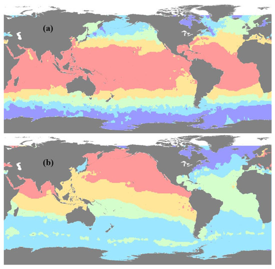
Figure 5.
Spatial partitioning results of global ocean DO for January. (a) represents 10 dbar and (b) represents 1000 dbar, with different colors indicating different partitions.
2.2.2. ML Training and Validation
The training dataset from BGC-Argo floats contained six variables: longitude, latitude, year, temperature, salinity, and DO. DO was the response variable, while the other five were predictors. We chose temperature and salinity as predictors because warmer water tends to hold less oxygen, and salinity also affects the solubility of oxygen in water [3]. Because all six variables were simultaneously observed by the floats at the same location, they have high spatiotemporal consistency and can be reliably used for model training. During the training process, the idea of spatial partitioning was emphasized to better capture the spatial variation in the data. By partitioning the data based on these criteria, the models can effectively learn and generalize patterns specific to different regions, depths, and time periods. Furthermore, the spatial partitioning approach introduces prior knowledge in regions with sparse training data, which aids in enhancing the model’s accuracy in these areas.
The training to test ratio was 4:1. Independent ML models were trained for each depth layer, month, and spatial partition. The grid search method was used to adjust the hyperparameters of the ML model, which is an optimization technique for ML models. It identifies the best model configuration by methodically exploring various combinations of hyperparameters. Different hyperparameter combinations were evaluated using the 3-fold cross-validation method, and the root-mean-square error (RMSE) loss function was used as the main evaluation metric to determine the best hyperparameter combinations. L2 regularization added a penalty term to the loss function during training to limit model complexity and prevent overfitting. This allowed the model to maintain simplicity while still learning useful patterns and improving generalization.
The performance of the TSD-ML model was evaluated in comparison to the test set. For each depth layer and month, multiple partitioned models were created based on the spatial partitions and tested independently. Due to the large number of models, overall accuracy was calculated based on the weighted average of the number of test set samples in each partition. The coefficient of determination R-squared (R2), RMSE, and mean absolute error (MAE) were used to evaluate performance:
where represents the actual observed DO value for the th sample, represents the reconstructed DO value for the th sample, denotes the mean value of all observed DO values, and is the total number of observed samples.
3. Results
3.1. Model Performance
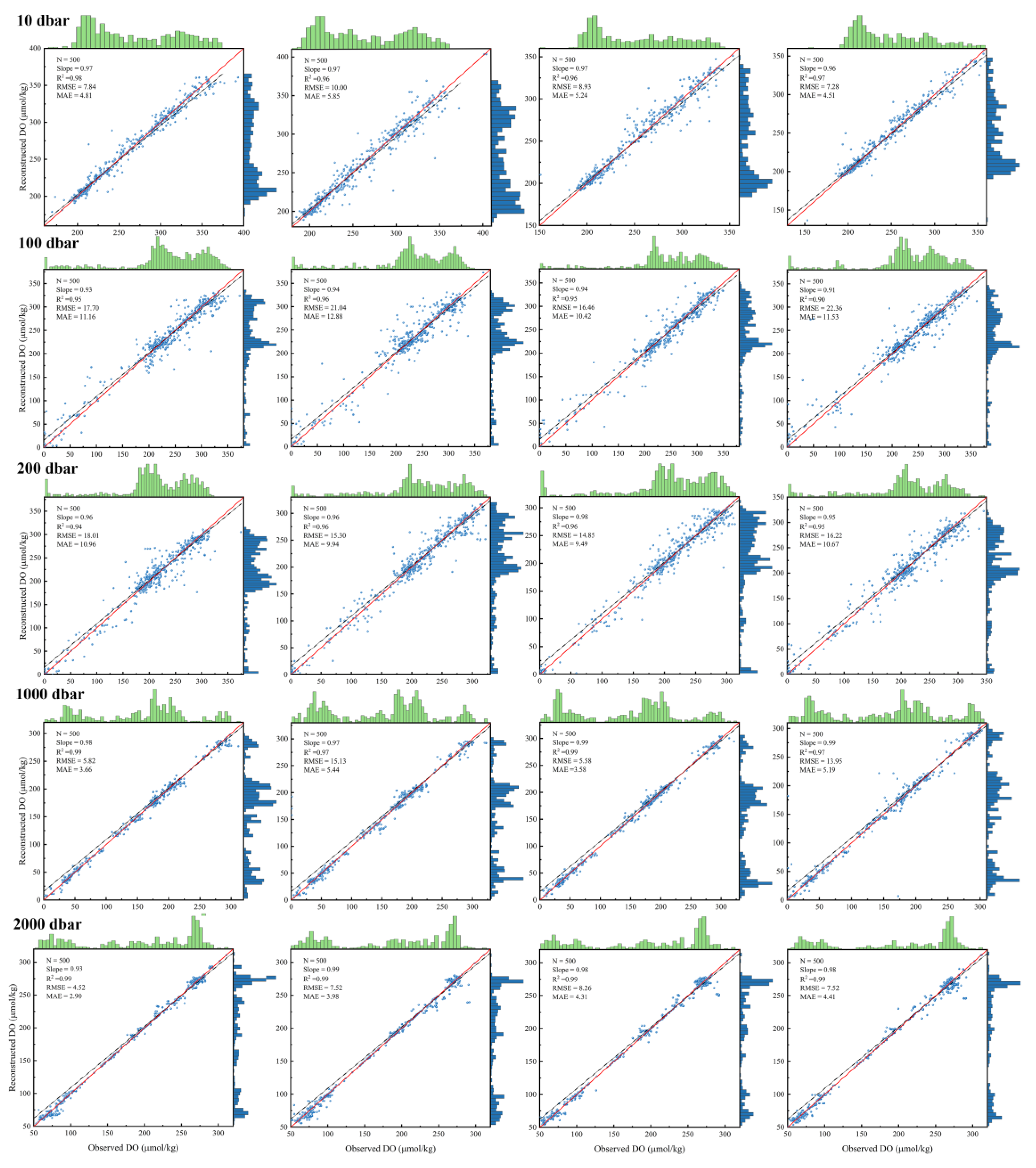
To verify the accuracy of the DO reconstruction results, 500 independent BGC Argo observations were randomly selected from five different layers (10, 100, 200, 1000, and 2000 dbar) in each of four months (January, April, July, and October). This random selection process was designed to ensure the representativeness of the test samples. The monthly DO reconstruction values were first interpolated to the global ocean grid using the SWP interpolation method. By mapping the spatial location of these 500 observations, the corresponding grid values in the reconstructed interpolation results were identified for comparison (Figure 6). As can be seen in the figure, the reconstructed values obtained by the TSD-ML model show an oscillating density distribution with a strong linear relationship with the observed values. Most RMSE values were within 15 μmol/kg, while MAE values were below 10 μmol/kg and R2 values were consistently above 0.9. Reconstruction results were best at 2000 dbar with an average RMSE of 6.95, MAE of 3.90, and R2 of 0.98. The lowest performance was at 100 dbar, with an average RMSE of 19.39, MAE of 10.27, and R2 of 0.95. High accuracy was also achieved at 10 dbar (RMSE 8.51, MAE 5.10, R2 0.97), 200 dbar (RMSE 16.10, MAE 10.27, R2 0.95), and 1000 dbar (RMSE 10.12, MAE 4.47, R2 0.98), illustrating the effectiveness of the hierarchical modeling approach.
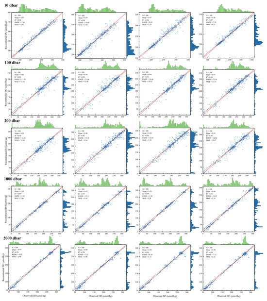
Figure 6.
Comparison of reconstructed DO with observed DO obtained from BGC-Argo floats. The months are arranged sequentially from left to right, specifically January, April, July, and October. The solid red line and dashed black line in each plot represent the 1:1 line and the linear fit, respectively. The marginal histograms on the plot describe the density distribution of observed (green) and reconstructed (blue) DO data points.
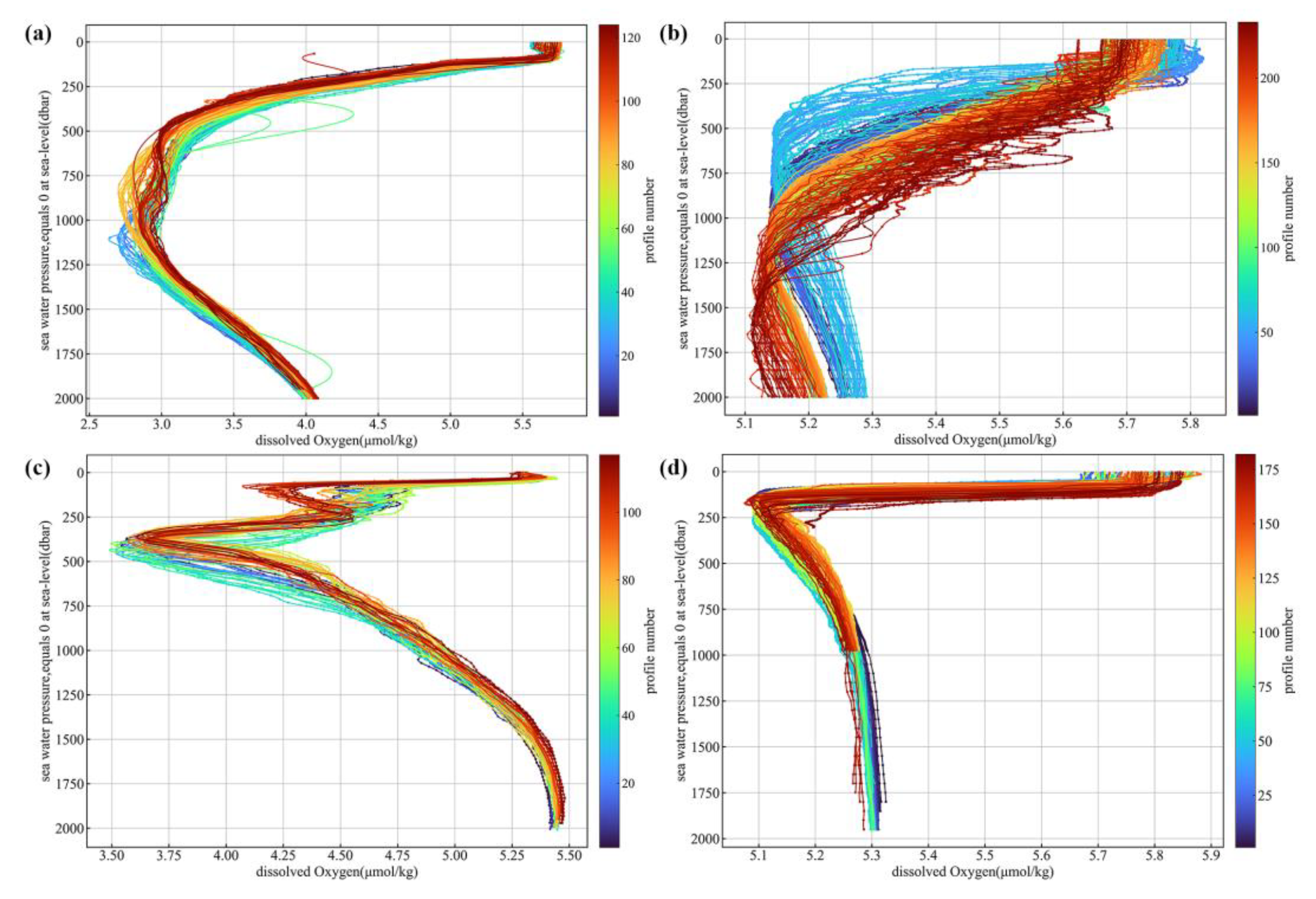
The relative error and its percentage are calculated using the above observed and reconstructed values. Table 1 shows that over 90% of the reconstructed data had relative errors within 10% for four months at 10 dbar and 2000 dbar layers. At 1000 dbar, about 85% were within 10%. The 100 dbar and 200 dbar layers performed less satisfactorily, with over 80% within 10%. The proportion of data with a relative error greater than 10% increased rapidly from the sea surface downwards, peaking in the 100 to 200 dbar range and gradually decreasing thereafter. This pattern can be attributed to the irregular variations in oceanic water properties at the base of the mixed layer or below. In contrast, below 200 dbar, where the water is generally in a stratified state, the regularity of oceanic changes stabilizes with increasing depth. Analysis of DO profiles from several BGC Argo floats revealed that in many regions (Figure 7) there is a large gradient of DO change with depth over the depth range of 100 dbar to 250 dbar. These variations are likely to be closely related to changes in mixed layer depth and changes in the respiration process of organic matter. However, the existing data in this depth range are insufficient to comprehensively explain these drastic changes, making it difficult to establish robust relationships between input variables and DO in this depth range.

Table 1.
Relative Error Table for TSD-CatBoost.

Figure 7.
Depth profiles of DO observed by Argo floats. Each panel corresponds to a specific float ID, and different colors represent different cycles. (a) Float ID: 4900523, located in the North Pacific Ocean. (b) Float ID: 5904481, located in the South Pacific Ocean. (c) Float ID: 6900629, located in the Atlantic Ocean. (d) Float ID: 5904671, located in the Indian Ocean.
The accuracy of the reconstruction results is confirmed by comparison with the observed values, indicating that the TSD-ML model has strong accuracy. As it is a data-driven model, additional training data is expected to further enhance performance at 100–200 dbar [42,43]. Overall, the TSD-ML model demonstrated excellent proficiency in estimating ocean DO.
3.2. Comparative Validation
This study includes a comparative analysis of the reconstructed DO with existing DO datasets, namely WOA18 and GLODAPv2, to evaluate the accuracy of the reconstructed data.
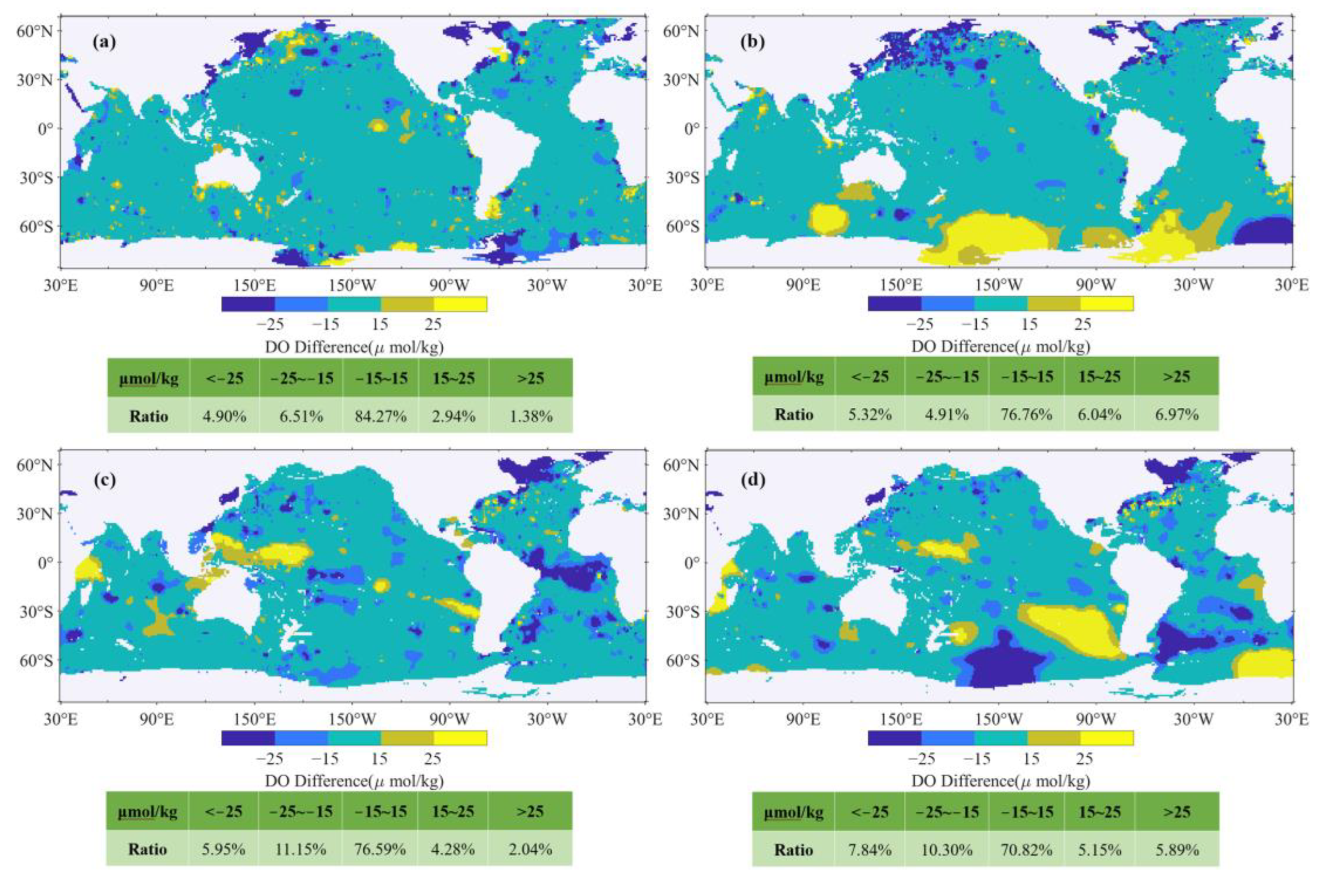
The WOA18 dataset, an authoritative source of historical DO records since 1950, features a 1° × 1° spatial resolution and provides climatological monthly scale data. To facilitate comparisons on a uniform scale, this study transformed the reconstructed DO data to match the spatiotemporal resolution of the WOA18 DO. The differences between the reconstructed DO data and the WOA18 data were then quantitatively assessed by calculating the grid differences between them. Taking the comparison at 10 dbar and 1000 dbar in January and July as examples (Figure 8), we found that the absolute error in DO mostly stayed within 15 μmol/kg across the majority of global oceanic regions. The analysis underscored high spatial agreement with WOA18, though notable disparities were observed in coastal zones and parts of the Southern Ocean. These discrepancies are likely attributable to the differing time periods covered by the datasets and the different ways in which the data were developed. First, there is a significant difference in the time periods covered by the respective datasets. The WOA18 dataset encompasses a historical range from 1950 to 2018, thereby capturing oceanic DO levels across a span of nearly seven decades. In contrast, the reconstructed DO data in our study are confined to the period from 2005 to 2022. This narrower, more contemporary timeframe means that the reconstructed data reflect more recent oceanographic and climatic conditions. Second, the methodologies employed in developing these datasets are different. The WOA18 dataset is compiled through an objective analysis of all accumulated shipboard data. In contrast, the DO dataset in our study is obtained by jointly interpolating both reconstructed and original Argo DO data. Additionally, the Argo DO data is relatively sparse in coastal regions, yet densely distributed in the Southern Ocean (Figure 1a). This disparity in data distribution and collection methods between the two datasets inevitably contributes to the differences observed in the study.
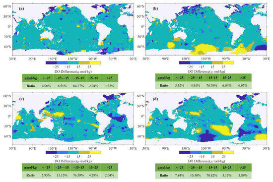
Figure 8.
Comparison of differences between 10dbar and 1000dbar layers reconstructed DO and WOA18 DO for January and July. Subfigures: (a) 10 dbar January, (b) 10 dbar July, (c) 1000 dbar January, (d) 1000 dbar July.
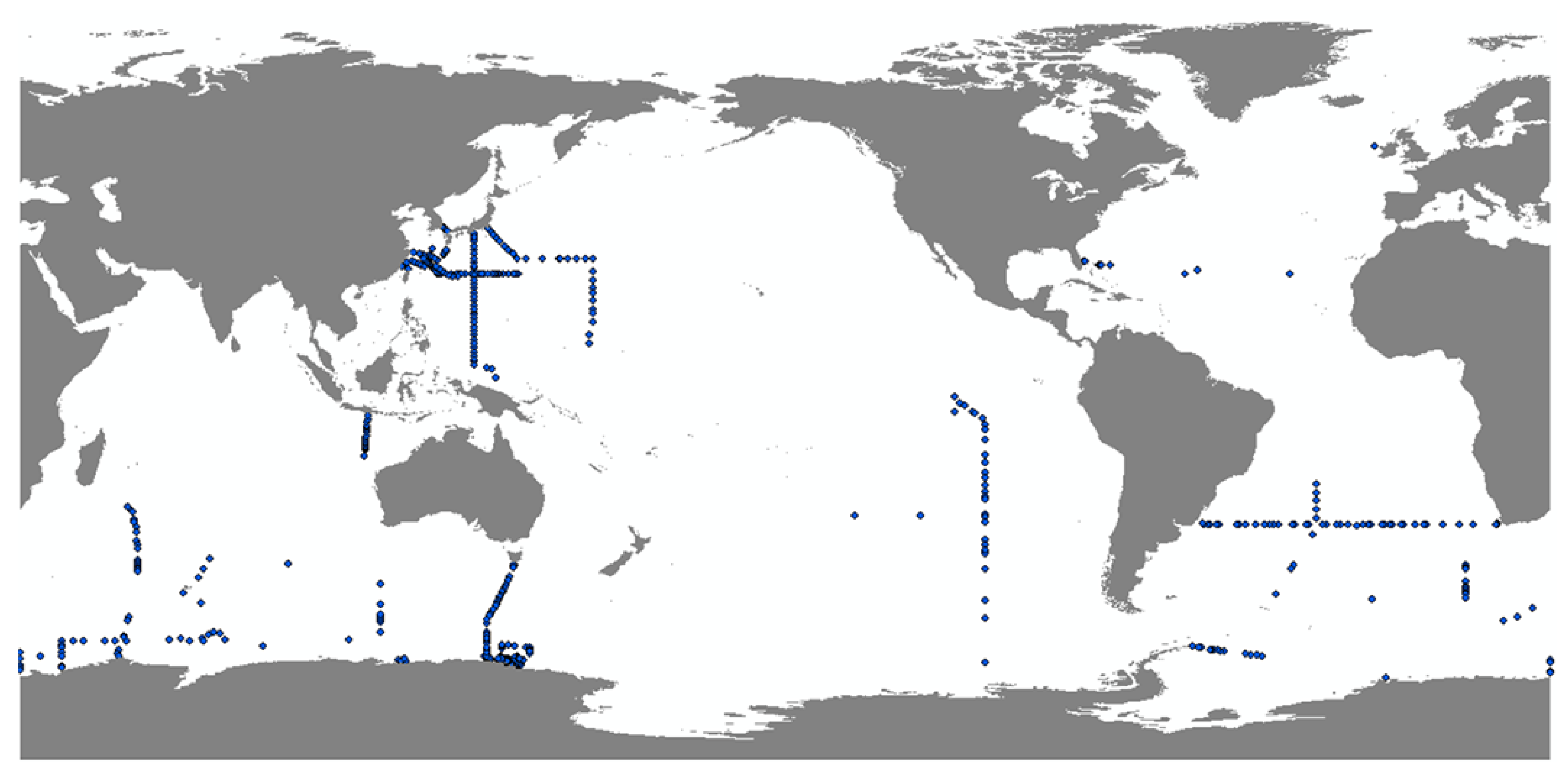
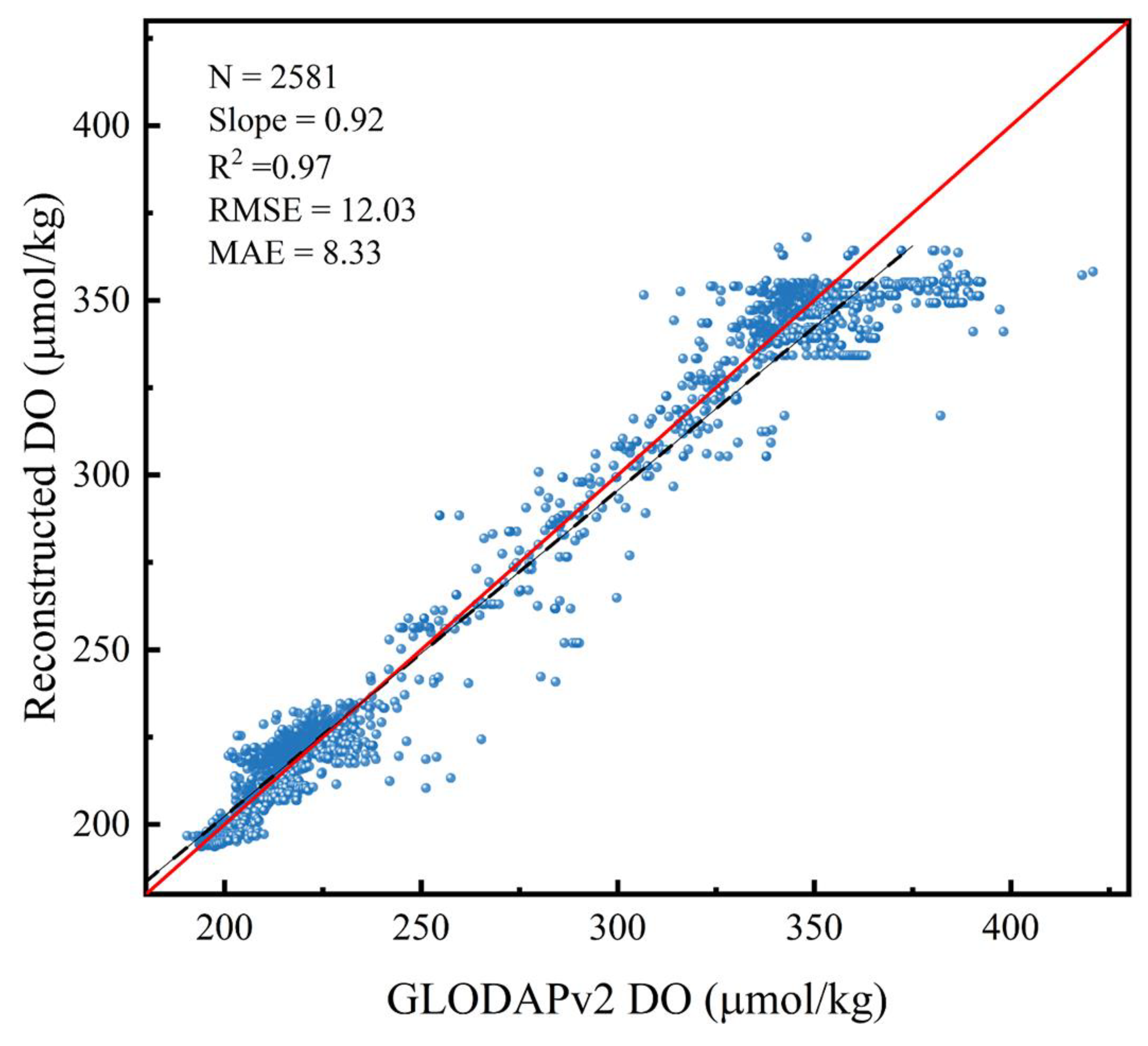
For further assessment on a monthly scale, we selected GLODAPv2 observations from the 10 dbar layer from January 2005 to 2021 (Figure 9). The GLODAP v2 dataset relies mainly on observations from research vessels, among which the DO data is the most representative biogeochemical variable in the GLODAPv2 dataset with a high degree of quality control. The latest GLODAPv2 dataset, covering DO data from 1970 to 2021, served as a valuable reference. The comparative analysis of the reconstructed DO at a 10 dbar layer for January between 2005 and 2021 showed a strong linear correlation with the GLODAPv2 observations, as evidenced by an R2 value of 0.97 (Figure 10). A statistical analysis comparing the reconstructed DO with GLODAPv2 DO across multiple years is summarized in Table 2. It was observed that in 2005 and 2010, 92.1% of the data had relative errors within 5%. In 2015 and 2020, 77.6% and 76.9% of the data maintained relative errors below 5%, respectively. These findings underscore the high consistency between the reconstructed and GLODAPv2 DO data, thereby corroborating the precision of the DO reconstruction via the TSD-ML method.
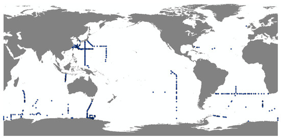
Figure 9.
Distribution map of GLODAPv2 DO data at 10 dbar in January.
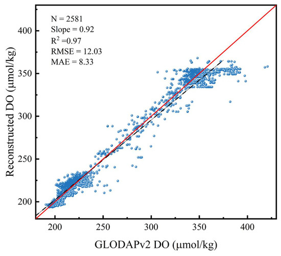
Figure 10.
Scatter plot comparing reconstructed DO values with GLODAPv2 data.
Table 2.
Statistical table of relative errors between GLODAPv2 and reconstruction results.
4. Discussion
4.1. Advantage of Spatial Partition
This study focuses on five distinct layers (10, 100, 200, 1000, and 2000 dbar) across four months (January, April, July, and October) to assess the partitioning modeling efficacy of the TSD-ML. The performance was evaluated using RMSE and MAE as metrics.
The study explores the effectiveness of spatial partitioned (SP) modeling, contrasting it with two alternative methodologies. The first approach, non-spatial partitioning (NSP), directly inputs the time–depth partitioned dataset into the ML model, without considering spatial partitioning. The second approach, partitioning as input variables (PIV), incorporates spatial partition labels as predictors of the model. This paper compares the predictive accuracy of the three partitioning strategies (SP, NSP, and PIV) using three ML algorithms: CatBoost [44], RF, and SVR. The comparative analysis is detailed in Table 3. The relevant results of RF and SVR are shown in Appendix A and Table A1 and Table A2.
Table 3.
Comparison of spatial partitioned (SP), partitioning as input variables (PIV), and non-spatial partitioning (NSP) approaches using the CatBoost algorithm.
Comparative analysis of modeling approaches on the test set indicated that SP modeling yielded the highest accuracy. Utilizing the CatBoost algorithm, SP’s average RMSE and MAE were 31.05% and 20.16% lower than NSP, and 31.64% and 20.49% lower than PIV, respectively. Similar trends were observed with RF and SVR models, reinforcing the efficacy of SP modeling.
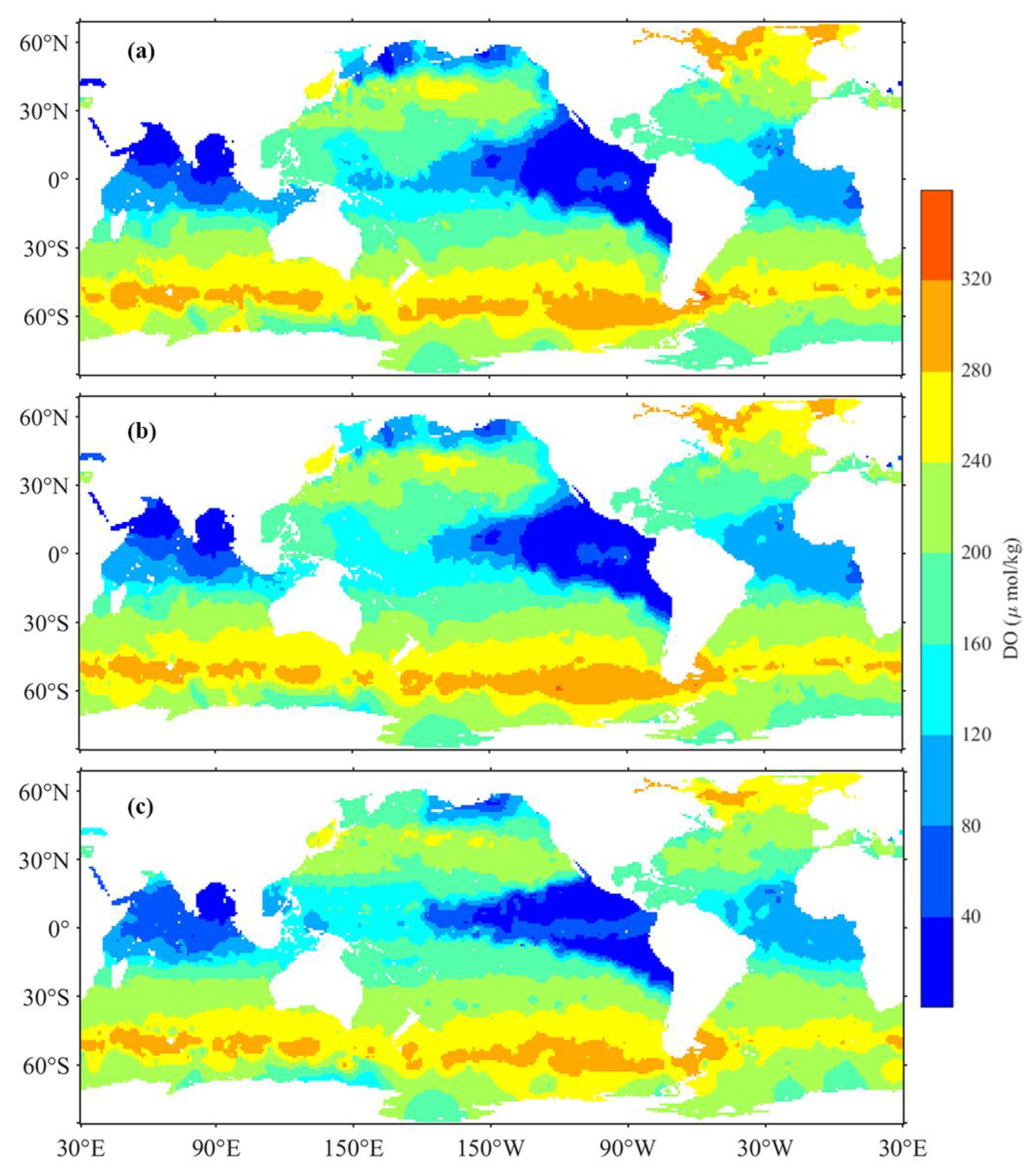
Furthermore, this study selected the 200 dbar layer reconstruction data in January 2010 for visualization (Figure 11). It facilitates the comparison of the reliability of reconstruction results from different modeling approaches. The reconstructions from PIV and SP models demonstrated closer resemblance, in contrast to those from NSP. NSP’s results prominently featured latitude and strip patterns in the spatial distribution of DO, which is inconsistent with DO’s actual distribution influenced by multiple complex environmental factors. Thus, omitting spatial partitioning in modeling significantly affects the accuracy of the reconstruction outcomes.
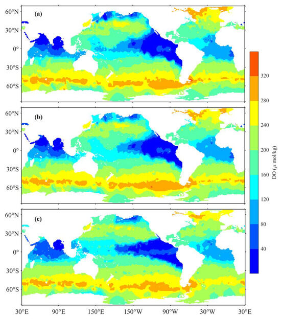
Figure 11.
Distribution maps of DO at 200 dbar in January modeled using SP (a), PIV (b), and NSP (c) methods.
The overall accuracy of the SP approach on the five depth layers and 4-month test set performs well. Taking the CatBoost model as an example, the accuracy of the 1000 dbar and 2000 dbar layers is particularly prominent, and the RMSE and MAE values of each month are relatively low. The 2000 dbar layer has the highest accuracy, the RMSE is less than 4 μmol/kg, and the MAE is close to 2 μmol/kg. Overall, despite increasing the total number of models, the SP approach is instrumental in markedly enhancing overall reconstruction accuracy. Demonstrating high reconstruction precision across various test depth layers and months, the SP method consistently shows low RMSE and MAE. These experimental outcomes underscore the substantial benefits of the spatial partitioning approach introduced in this study for improving the accuracy of DO reconstruction.
4.2. Sensitivity Test
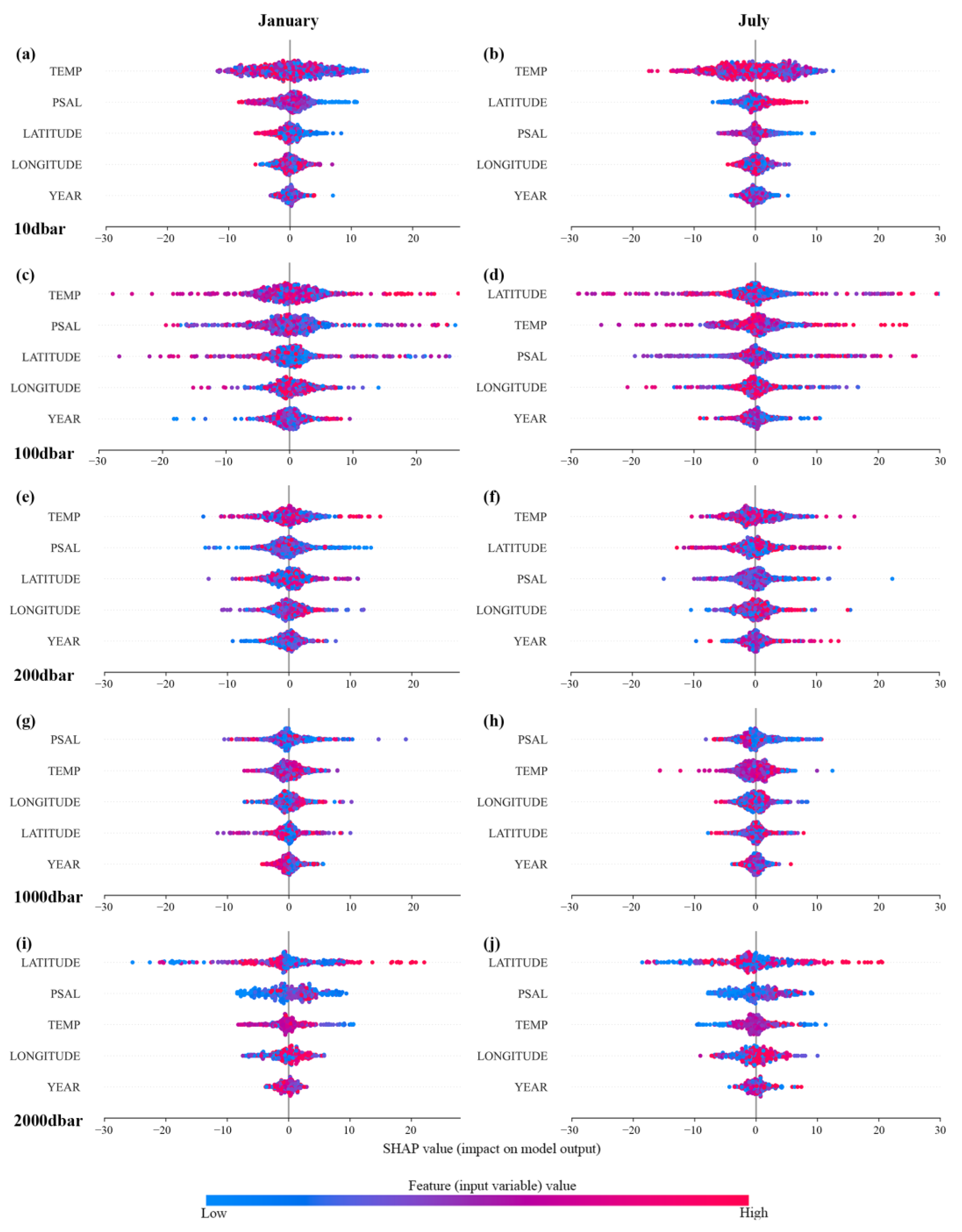
The SHAP (SHapley Additive exPlained) analysis was used to interpret model variable importance [45]. The SHAP computes the significance of input variables in the TSD-CatBoost model. Briefly, to estimate DO response, the TSD-CatBoost model generates a SHAP value for each input variable. The SHAP value summary plot combines feature importance with feature effects. In this way, a large range of SHAP values indicate that the variable has the greatest influence on predicted DO (Figure 12). The x-axis of the plot specifies the SHAP value, signifying the impact of each variable on model predictions. Positive values denote positive effects, while negative values suggest negative ones. The y-axis organizes input variables by their cumulative effect on the predicted DO, ranked in descending order. The most influential variable is positioned at the top. Each plot dot signifies an individual training sample, with dot colors indicating the feature values (input variables) from low to high.
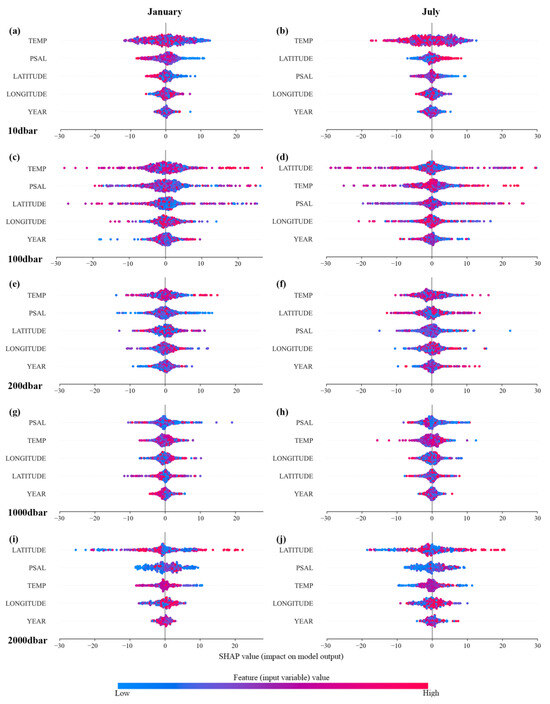
Figure 12.
The SHAP summary plots of the test dataset trained with the CatBoost model at 10 dbar (a,b), 100 dbar (c,d), 200 dbar (e,f), 1000 dbar (g,h), and 2000 dbar (i,j). The left side of each row represents January (winter) and the right side represents July (summer).
Analytical results indicate that, in winter, temperature and salinity exert the most significant influence on DO at the layers of 10 dbar, 100 dbar, and 200 dbar. Variations in temperature lead to maximum changes in DO, approximately ranging from −15 to 15 µmol/kg at 10 dbar, −30 to 30 µmol/kg at 100 dbar, and −15 to 15 µmol/kg at 200 dbar. At the 1000 dbar layer, temperature and salinity continue to serve as principal regulatory factors in both seasons. At the 2000 dbar layer, latitude emerges as the predominant predictive factor. Despite this, temperature and salinity remain potentially significant factors influencing DO in the deep ocean. The distribution of SHAP values for each variable reveals distinct patterns where certain variables demonstrate divergent associations between SHAP values and input variables across different months. For instance, the relationship between latitude and DO in winter and summer differs at the 10 dbar layer (Figure 12a,b). In winter, a decrease in latitude resulted in an increase in DO, while an increase in latitude caused a decrease in DO. However, in summer, this relationship becomes inverted. The distribution of SHAP value for each variable suggests that some variables exhibit nonlinear relationships between SHAP values and input variables. For instance, the salinity at 200 dbar in January (Figure 12e) is not in a linear relationship with DO, where increases in the SHAP value lead to consistent changes in model prediction. The effect of low salinity on DO varies, potentially being either positive or negative. These variable-DO relationships demonstrated the complex factors influencing DO distributions.
4.3. Global DO Trends
Reconstructed DO data are integrated with observed DO data sourced from the BGC-Argo floats. These merged data were then interpolated into 1° × 1° global monthly grids from 2005–2022 across 26 depth layers. Analyses concentrated on 12 specific depth levels (shown in Figure 13), considering the variability of DO in upper ocean layers and the stability in lower layers.
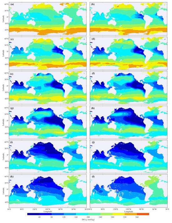
Figure 13.
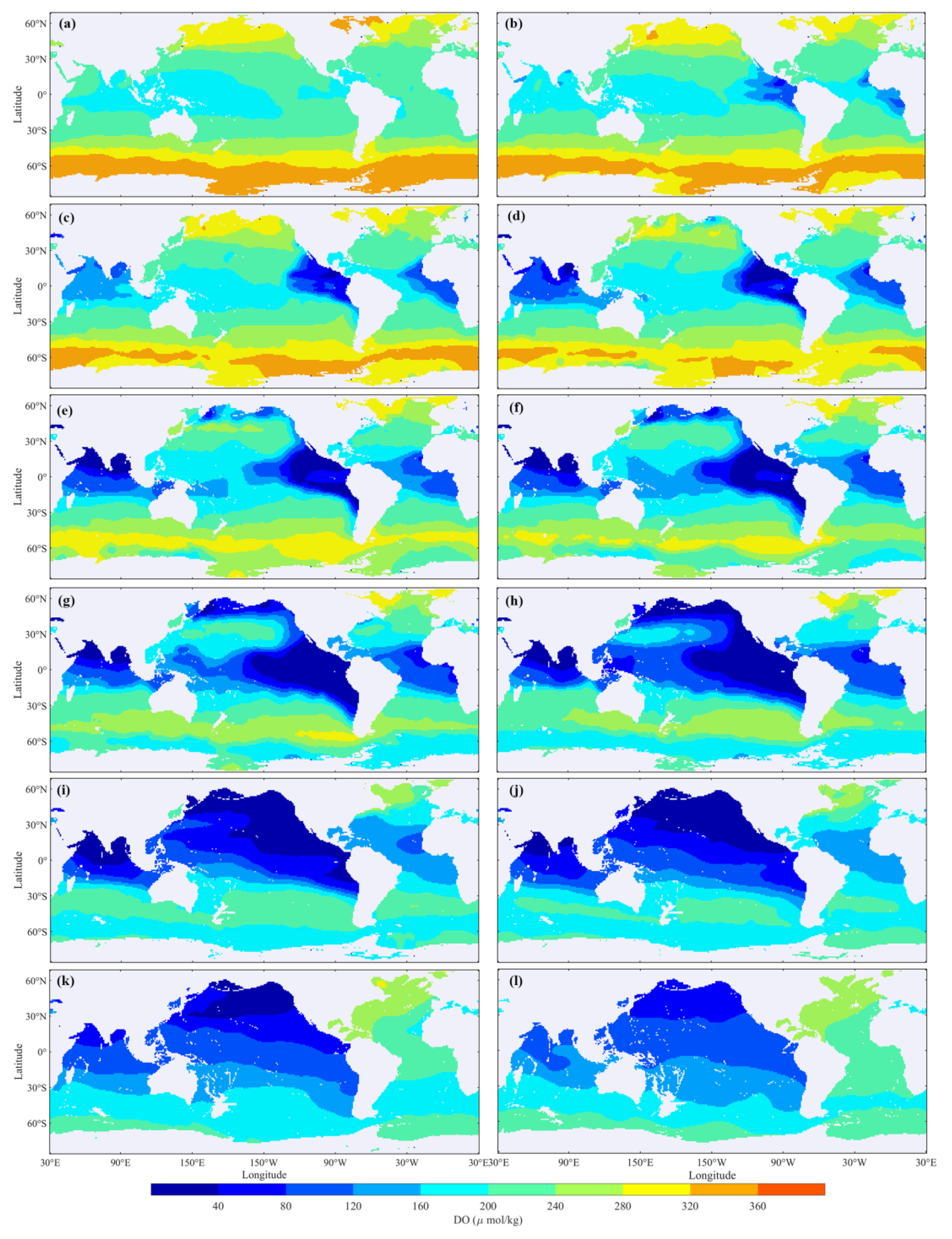
Ocean Annual Average DO Distribution at Various Depths: (a) 10 dbar, (b) 50 dbar, (c) 75 dbar, (d) 100 dbar, (e) 150 dbar, (f) 200 dbar, (g) 300 dbar, (h) 500 dbar, (i) 800 dbar, (j) 1000 dbar, (k) 1500 dbar, (l) 2000 dbar.
Observations indicate significant spatial and depth-related variability in global ocean DO. Generally, DO levels decrease and then increase with depth. Hypoxic zones predominantly arise in the equatorial eastern Pacific Ocean and the northern Indian Ocean, expanding with depth. Between 100 and 500 dbar, a decrease in DO and expansion of low oxygen zones are noted, particularly in the north Indian Ocean and the equatorial east Pacific Ocean. Between 500 and 1000 dbar, while hypoxic areas contract in the north Indian Ocean, notable hypoxia remains in the north Pacific and equatorial east Pacific Oceans, with northward movement of the anoxic zone. Between 1000 and 2000 dbar, a global DO recovery is evident, especially in the Atlantic Ocean. DO distribution in both the Indian and Pacific Oceans shows lower levels in northern and higher levels in southern regions, with the anoxic zone almost disappearing near 2000 dbar.
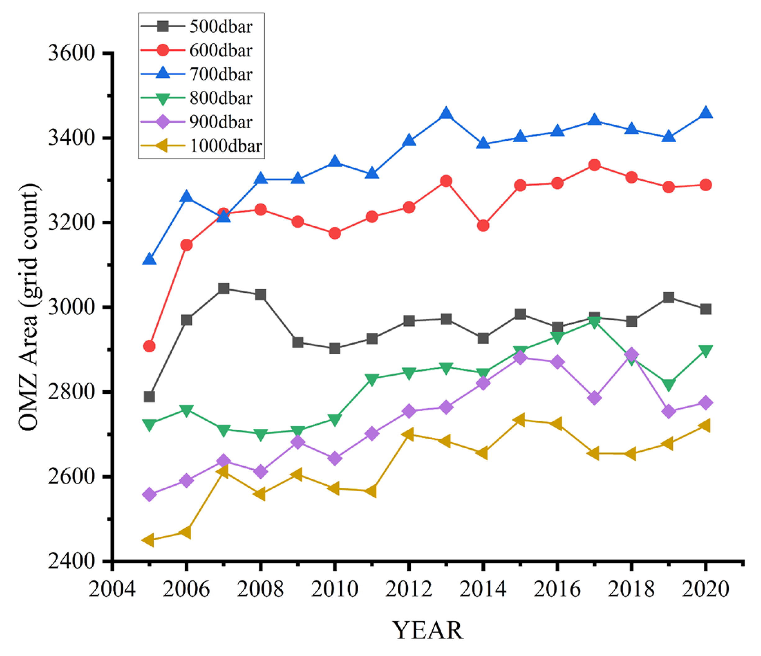
The study presents a preliminary statistical analysis of the interannual variability in the area of the oxygen minimum zones (OMZs) at various depth layers using reconstructed DO (Figure 14). It quantifies the interannual changes in the OMZs area (represented by grid counts (1° × 1°)) at 500–1000 dbar. There is no definite threshold for the definition of the maximum value of the OMZs range, varying from 20 to 60 μmol/kg [46]. This paper defines the range of OMZs as 0~26 μmol/kg. A global increase in DO hypoxia, especially between 600 and 700 dbar, is observed. Statistical analyses have deduced that the annual mean growth rates of the OMZs areas at the depths of 500 dbar, 600 dbar, 700 dbar, 800 dbar, 900 dbar, and 1000 dbar from 2005 to 2020 are, respectively, 0.50%, 0.85%, 0.72%, 0.43%, 0.56%, and 0.72%. These rates exceed 0.4%, with an average annual rate of 0.63%, indicating an increasing deoxygenation of the global ocean. This trend of rising deoxygenation rates is particularly alarming, as it suggests a worsening of hypoxic conditions in the ocean, potentially impacting marine life.
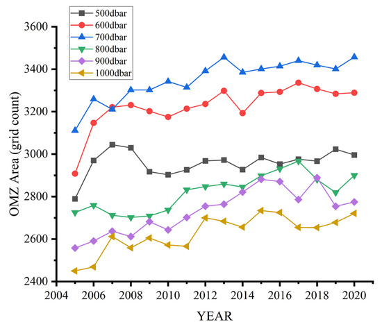
Figure 14.
Quantitative analysis of global ocean OMZs area across various depth layers (2005–2020).
5. Conclusions
This paper proposes a method for reconstructing the global ocean DO model based on time–space–depth partitioning, aiming to improve the reconstruction accuracy of the model in areas with sparse data and uneven distribution, thereby providing a basis for understanding the distribution and dynamic changes in global ocean DO. The method involved partitioning Argo DO data along time, depth, and space, and developing an ML model for each partition. The main conclusions are as follows:
- (1)
- The TSD-ML method demonstrates commendable performance in the reconstruction of DO. The spatial heterogeneity of DO is fully considered when training ML models.
- (2)
- Partition modeling significantly improves the reconstruction accuracy of the model. Compared to the NSP and PIV approaches, the SP approach significantly improves model performance in data-sparse areas, which will promote the applications of ML in the marine domain.
- (3)
- The comparative analysis of the reconstructed DO with WOA18 and GLODAPv2 ship survey DO demonstrates a high degree of spatial consistency. This validation underscores the effectiveness of our approach in accurately depicting global ocean DO.
For future spatiotemporal analyses, integrating additional datasets such as GLODAPv2 DO data is recommended to enhance precision and provide a more comprehensive understanding of global ocean DO dynamics.
Author Contributions
Z.W. drafted the initial version, prepared the manuscript with input from B.P., coordinated, and contributed to the edits of all sections. C.X. significantly improved the paper through thorough editorial revisions. All authors have read and agreed to the published version of the manuscript.
Funding
This research was jointly funded by the Innovative Research Program of the International Research Center of Big Data for Sustainable Development Goals (No. CBAS2022IRP05) and by National Natural Science Foundation of China (No.42376193). Additionally, the APC was funded by CBAS2022IRP05.
Data Availability Statement
All original code has been deposited at Github (https://github.com/layne1202/SP_DO_Reconstruction, accessed on 29 August 2023). Monthly DO datasets generated in this study have been deposited at Zenodo (https://zenodo.org/records/10147890, accessed on 17 November 2023).
Conflicts of Interest
The authors declare that there are no conflicts of interest in this study. The funders had no role in the design of the study; in the collection, analysis, or interpretation of data; in the writing of the manuscript; or in the decision to publish the results.
Appendix A
Table A1.
Comparison of SP, PIV, and NSP approaches using the random forest regression (RF) algorithm.
Table A1.
Comparison of SP, PIV, and NSP approaches using the random forest regression (RF) algorithm.
| Depth | Month | RMSE | MAE | ||||
|---|---|---|---|---|---|---|---|
| SP | PIV | NSP | SP | PIV | NSP | ||
| 10 dbar | 1 | 4.14 | 10.43 | 11.07 | 2.87 | 3.61 | 3.88 |
| 4 | 4.87 | 5.84 | 5.88 | 3.17 | 3.6 | 3.67 | |
| 7 | 4.71 | 6.07 | 6.01 | 2.97 | 3.58 | 3.63 | |
| 10 | 4.36 | 5.81 | 6.15 | 2.88 | 3.17 | 3.27 | |
| 100 dbar | 1 | 10.26 | 14.62 | 14.08 | 6.7 | 7.72 | 8.09 |
| 4 | 8.71 | 11.18 | 13.36 | 5.42 | 6.43 | 6.85 | |
| 7 | 8.88 | 11.44 | 14.96 | 5.75 | 6.65 | 7.18 | |
| 10 | 9.47 | 15.01 | 12.33 | 5.89 | 6.91 | 7.03 | |
| 200 dbar | 1 | 7.29 | 10.67 | 15.3 | 4.99 | 6.21 | 7.34 |
| 4 | 6.98 | 11.47 | 11.94 | 4.57 | 6.31 | 6.54 | |
| 7 | 7 | 9.37 | 10.45 | 4.57 | 5.59 | 5.94 | |
| 10 | 7.37 | 11.18 | 11.54 | 4.92 | 6.47 | 6.42 | |
| 1000 dbar | 1 | 2.72 | 5.18 | 4.13 | 1.88 | 2.18 | 2.11 |
| 4 | 3.08 | 3.58 | 3.43 | 1.97 | 2.13 | 2.2 | |
| 7 | 2.95 | 3.68 | 3.65 | 1.81 | 2.21 | 2.13 | |
| 10 | 2.85 | 3.73 | 4.52 | 1.9 | 2.17 | 2.37 | |
| 2000 dbar | 1 | 3.29 | 3.81 | 6.68 | 2.17 | 2.41 | 3.26 |
| 4 | 3.4 | 4.17 | 4.09 | 2 | 2.35 | 2.42 | |
| 7 | 3.74 | 4.03 | 4.55 | 2.33 | 2.42 | 2.67 | |
| 10 | 3.81 | 4.53 | 5.32 | 2.26 | 2.45 | 2.81 | |
Table A2.
Comparison of SP, PIV and NSP approaches using the support vector regression (SVR) algorithm.
Table A2.
Comparison of SP, PIV and NSP approaches using the support vector regression (SVR) algorithm.
| Depth | Season | RMSE | MAE | ||||
|---|---|---|---|---|---|---|---|
| SP | PIV | NSP | SP | PIV | NSP | ||
| 10 dbar | 1 | 4.73 | 11.37 | 11.28 | 3.15 | 4.29 | 4.46 |
| 4 | 5.16 | 6.37 | 6.79 | 3.28 | 4.24 | 4.41 | |
| 7 | 5.31 | 6.72 | 6.65 | 3.29 | 4.36 | 4.35 | |
| 10 | 4.61 | 5.46 | 7.16 | 2.97 | 3.55 | 4.01 | |
| 100 dbar | 1 | 11.38 | 14.05 | 18.23 | 6.74 | 8.46 | 10.08 |
| 4 | 8.67 | 10.17 | 11.71 | 5.45 | 6.93 | 8.03 | |
| 7 | 8.79 | 12.99 | 13.6 | 5.51 | 7.84 | 8.36 | |
| 10 | 10.01 | 19.69 | 14.76 | 6.22 | 8.86 | 9.12 | |
| 200 dbar | 1 | 7.69 | 9.98 | 10.87 | 4.82 | 6.92 | 7.49 |
| 4 | 8.23 | 10.66 | 10.52 | 5.14 | 6.94 | 7.13 | |
| 7 | 7.77 | 9.81 | 10.48 | 4.57 | 6.81 | 7.01 | |
| 10 | 7.68 | 10.54 | 9.77 | 4.94 | 7.01 | 7.02 | |
| 1000 dbar | 1 | 3.35 | 5.81 | 5.52 | 1.90 | 4.27 | 4.41 |
| 4 | 3.05 | 5.19 | 5.25 | 1.86 | 4.09 | 4.05 | |
| 7 | 2.92 | 5.25 | 5.5 | 1.78 | 4.05 | 4.35 | |
| 10 | 2.95 | 4.88 | 5.85 | 1.80 | 3.85 | 4.47 | |
| 2000 dbar | 1 | 3.38 | 5.83 | 5.37 | 2.22 | 4.16 | 4.24 |
| 4 | 3.32 | 4.85 | 5.72 | 2.10 | 3.54 | 4.26 | |
| 7 | 4.21 | 5.19 | 5.84 | 2.54 | 3.91 | 4.27 | |
| 10 | 4.69 | 5.71 | 5.99 | 2.43 | 3.79 | 3.87 | |
References
- Varol, M. Use of water quality index and multivariate statistical methods for the evaluation of water quality of a stream affected by multiple stressors: A case study. Environ. Pollut. 2020, 266, 115417. [Google Scholar] [CrossRef] [PubMed]
- Song, H.J.; Wignall, P.B.; Song, H.Y.; Dai, X.; Chu, D.L. Seawater Temperature and Dissolved Oxygen over the Past 500 Million Years. J. Earth Sci. 2019, 30, 236–243. [Google Scholar] [CrossRef]
- Chi, L.B.; Song, X.X.; Yuan, Y.Q.; Wang, W.T.; Cao, X.H.; Wu, Z.X.; Yu, Z.M. Main factors dominating the development, formation and dissipation of hypoxia off the Changjiang Estuary (CE) and its adjacent waters, China. Environ. Pollut. 2020, 265, 115066. [Google Scholar] [CrossRef] [PubMed]
- Diaz, R.J.; Rosenberg, R. Spreading dead zones and consequences for marine ecosystems. Science 2008, 321, 926–929. [Google Scholar] [CrossRef] [PubMed]
- Vaquer-Sunyer, R.; Duarte, C.M. Thresholds of hypoxia for marine biodiversity. Proc. Natl. Acad. Sci. USA 2008, 105, 15452–15457. [Google Scholar] [CrossRef] [PubMed]
- Morée, A.L.; Clarke, T.M.; Cheung, W.W.L.; Frölicher, T.L. Impact of deoxygenation and warming on global marine species in the 21 stcentury. Biogeosciences 2023, 20, 2425–2454. [Google Scholar] [CrossRef]
- Kim, H.; Franco, A.C.; Sumaila, U.R. A Selected Review of Impacts of Ocean Deoxygenation on Fish and Fisheries. Fishes 2023, 8, 316. [Google Scholar] [CrossRef]
- Breitburg, D.; Levin, L.A.; Oschlies, A.; Gregoire, M.; Chavez, F.P.; Conley, D.J.; Garcon, V.; Gilbert, D.; Gutierrez, D.; Isensee, K.; et al. Declining oxygen in the global ocean and coastal waters. Science 2018, 359, eaam7240. [Google Scholar] [CrossRef]
- Zhang, X.D.; Wang, Z.L.; Cai, H.W.; Chai, X.P.; Tang, J.L.; Zhuo, L.F.; Jia, H.B. Summertime dissolved oxygen concentration and hypoxia in the Zhejiang coastal area. Front. Mar. Sci. 2022, 9, 1051549. [Google Scholar] [CrossRef]
- Kim, H.; Hirose, N.; Takayama, K. Physical and Biological Factors Underlying Long-Term Decline of Dissolved Oxygen Concentrationin the East/Japan Sea. Front. Mar. Sci. 2022, 9, 851598. [Google Scholar] [CrossRef]
- Simonovic, N.; Dominovic, I.; Margus, M.; Matek, A.; Ljubesic, Z.; Ciglenecki, I. Dynamics of organic matter in the changing environment of a stratified marine lake over two decades. Sci. Total Environ. 2023, 865, 161076. [Google Scholar] [CrossRef] [PubMed]
- Dimarco, S.F.; Wang, Z.K.; Chapman, P.; al-Kharusi, L.; Belabbassi, L.; al-Shaqsi, H.; Stoessel, M.; Ingle, S.; Jochens, A.E.; Howard, M.K. Monsoon-driven seasonal hypoxia along the northern coast of Oman. Front. Mar. Sci. 2023, 10, 1248005. [Google Scholar] [CrossRef]
- Eyring, V.; Bony, S.; Meehl, G.A.; Senior, C.A.; Stevens, B.; Stouffer, R.J.; Taylor, K.E. Overview of the Coupled Model Intercomparison Project Phase 6 (CMIP6) experimental design and organization. Geosci. Model Dev. 2016, 9, 1937–1958. [Google Scholar] [CrossRef]
- Kwiatkowski, L.; Torres, O.; Bopp, L.; Aumont, O.; Chamberlain, M.; Christian, J.R.; Dunne, J.P.; Gehlen, M.; Ilyina, T.; John, J.G.; et al. Twenty-first century ocean warming, acidification, deoxygenation, and upper-ocean nutrient and primary production decline from CMIP6 model projections. Biogeosciences 2020, 17, 3439–3470. [Google Scholar] [CrossRef]
- Ito, T. Optimal interpolation of global dissolved oxygen: 1965–2015. Geosci. Data J. 2022, 9, 167–176. [Google Scholar] [CrossRef]
- Schmidtko, S.; Stramma, L.; Visbeck, M. Decline in global oceanic oxygen content during the past five decades. Nature 2017, 542, 335–339. [Google Scholar] [CrossRef]
- Garcia, H.E.; Locarnini, R.A.; Boyer, T.P.; Antonov, J.I.; Johnson, D.R. Dissolved Oxygen, Apparent Oxygen Utilization, and Oxygen Saturation; NOAA Atlas NESDIS 70 Series; National Oceanic and and Atmospheric Administration: Silver Spring, MA, USA, 2013. [Google Scholar]
- Olsen, A.; Key, R.M.; van Heuven, S.; Lauvset, S.K.; Velo, A.; Lin, X.H.; Schirnick, C.; Kozyr, A.; Tanhua, T.; Hoppema, M.; et al. The Global Ocean Data Analysis Project version 2 (GLODAPv2)—An internally consistent data product for the world ocean. Earth Syst. Sci. Data 2016, 8, 297–323. [Google Scholar] [CrossRef]
- Lauvset, S.K.; Key, R.M.; Olsen, A.; van Heuven, S.; Velo, A.; Lin, X.H.; Schirnick, C.; Kozyr, A.; Tanhua, T.; Hoppema, M.; et al. A new global interior ocean mapped climatology: The 1° × 1° GLODAP version 2. Earth Syst. Sci. Data 2016, 8, 325–340. [Google Scholar] [CrossRef]
- Key, R.M.; Olsen, A.; Heuven, S.v.; Lauvset, S.K.; Velo, A.; Lin, X.; Schirnick, C.; Kozyr, A.; Tanhua, T.; Hoppema, M.; et al. Global Ocean Data Analysis Project, Version 2 (GLODAPv2); Carbon Dioxide Information Analysis Center, Oak Ridge National Laboratory, US Department of Energy: Oak Ridge, TN, USA, 2015. [Google Scholar]
- Karakaya, N.; Evrendilek, F. Monitoring and validating spatio-temporal dynamics of biogeochemical properties in Mersin Bay (Turkey) using Landsat ETM+. Environ. Monit. Assess. 2011, 181, 457–464. [Google Scholar] [CrossRef]
- Riser, S.C.; Freeland, H.J.; Roemmich, D.; Wijffels, S.; Troisi, A.; Belbeoch, M.; Gilbert, D.; Xu, J.P.; Pouliquen, S.; Thresher, A.; et al. Fifteen years of ocean observations with the global Argo array. Nat. Clim. Change 2016, 6, 145–153. [Google Scholar] [CrossRef]
- Bittig, H.C.; Maurer, T.L.; Plant, J.N.; Schmechtig, C.; Wong, A.P.S.; Claustre, H.; Trull, T.W.; Bhaskar, T.; Boss, E.; DallOlmo, G.; et al. A BGC-Argo Guide: Planning, Deployment, Data Handling and Usage. Front. Mar. Sci. 2019, 6, 502. [Google Scholar] [CrossRef]
- Matear, R.J.; Hirst, A.C. Long-term changes in dissolved oxygen concentrations in the ocean caused by protracted global warming. Global Biogeochem. Cycles 2003, 17, 35-1–35-20. [Google Scholar] [CrossRef]
- Garcia, H.E.; Keeling, R.F. On the global oxygen anomaly and air-sea flux. J. Geophys. Res.-Oceans 2001, 106, 31155–31166. [Google Scholar] [CrossRef]
- Zhao, N.; Fan, Z.M.; Zhao, M.M. A New Approach for Estimating Dissolved Oxygen Based on a High-Accuracy Surface Modeling Method. Sensors 2021, 21, 3954. [Google Scholar] [CrossRef] [PubMed]
- Jiang, Y.; Gou, Y.; Zhang, T.; Wang, K.; Hu, C.Q. A Machine Learning Approach to Argo Data Analysis in a Thermocline. Sensors 2017, 17, 2225. [Google Scholar] [CrossRef] [PubMed]
- Sauzede, R.; Claustre, H.; Uitz, J.; Jamet, C.; Dall'Olmo, G.; D’Ortenzio, F.; Gentili, B.; Poteau, A.; Schmechtig, C. A neural network-based method for merging ocean color and Argo data to extend surface bio-optical properties to depth: Retrieval of the particulate backscattering coefficient. J. Geophys. Res.-Oceans 2016, 121, 2552–2571. [Google Scholar] [CrossRef]
- Yuan, Q.; Shen, H.; Li, T.; Li, Z.; Li, S.; Jiang, Y.; Xu, H.; Tan, W.; Yang, Q.; Wang, J.; et al. Deep learning in environmental remote sensing: Achievements and challenges. Remote Sens. Environ. 2020, 241, 111716. [Google Scholar] [CrossRef]
- Giglio, D.; Lyubchich, V.; Mazloff, M.R. Estimating Oxygen in the Southern Ocean Using Argo Temperature and Salinity. J. Geophys. Res.-Oceans 2018, 123, 4280–4297. [Google Scholar] [CrossRef]
- Sharp, J.D.; Fassbender, A.J.; Carter, B.R.; Johnson, G.C.; Schultz, C.; Dunne, J.P. GOBAI-O2: Temporally and spatially resolved fields of ocean interior dissolved oxygen over nearly two decades. Earth Syst. Sci. Data Discuss. 2022, 15, 4481–4518. [Google Scholar] [CrossRef]
- Wang, L.H.; Jiang, Y.; Qi, H. Marine Dissolved Oxygen Prediction with Tree Tuned Deep Neural Network. IEEE Access 2020, 8, 182431–182440. [Google Scholar] [CrossRef]
- Sagan, V.; Peterson, K.T.; Maimaitijiang, M.; Sidike, P.; Sloan, J.; Greeling, B.A.; Maalouf, S.; Adams, C. Monitoring inland water quality using remote sensing: Potential and limitations of spectral indices, bio-optical simulations, machine learning, and cloud computing. Earth Sci. Rev. 2020, 205, 103187. [Google Scholar] [CrossRef]
- Xiong, Y.J.; Ran, Y.L.; Zhao, S.H.; Zhao, H.; Tian, Q.X. Remotely assessing and monitoring coastal and inland water quality in China: Progress, challenges and outlook. Crit. Rev. Environ. Sci. Technol. 2020, 50, 1266–1302. [Google Scholar] [CrossRef]
- Palmer, S.C.J.; Kutser, T.; Hunter, P.D. Remote sensing of inland waters: Challenges, progress and future directions. Remote Sens. Environ. 2015, 157, 1–8. [Google Scholar] [CrossRef]
- Yu, X.; Shen, J.; Du, J.B. A Machine-Learning-Based Model for Water Quality in Coastal Waters, Taking Dissolved Oxygen and Hypoxia in Chesapeake Bay as an Example. Water Resour. Res. 2020, 56, e2020WR027227. [Google Scholar] [CrossRef]
- Ross, A.C.; Stock, C.A. An assessment of the predictability of column minimum dissolved oxygen concentrations in Chesapeake Bay using a machine learning model. Estuar. Coast. Shelf S 2019, 221, 53–65. [Google Scholar] [CrossRef]
- Heddam, S.; Kim, S.; Mehr, A.D.; Kermani, Z.; Malik, A.; Elbeltagi, A.; Kisi, O. Predicting dissolved oxygen concentration in river using new advanced machines learning: Long-short term memory (LSTM) deep learning. In Computers in Earth and Environmental Sciences; Elsevier: Amsterdam, The Netherlands, 2022; pp. 1–20. [Google Scholar]
- Moghadam, S.V.; Sharafati, A.; Feizi, H.; Marjaie, S.M.S.; Asadollah, S.; Motta, D. An efficient strategy for predicting river dissolved oxygen concentration: Application of deep recurrent neural network model. Environ. Monit. Assess. 2021, 193, 798. [Google Scholar] [CrossRef]
- Sun, J.; Li, D.; Fan, D. A novel dissolved oxygen prediction model based on enhanced semi-naive Bayes for ocean ranches in northeast China. PeerJ Comput. Sci. 2021, 7, e591. [Google Scholar] [CrossRef]
- Li, H.; Xu, J.P.; Liu, Z.H.; Sun, Z.H. Study on the establishment of gridded Argo data by successive orrection. Marin. Sci. Bull. 2012, 31, 502–514. [Google Scholar] [CrossRef]
- Cao, Z.G.; Ma, R.H.; Duan, H.T.; Pahlevan, N.; Melack, J.; Shen, M.; Xue, K. A machine learning approach to estimate chlorophyll-a from Landsat-8 measurements in inland lakes. Remote Sens. Environ. 2020, 248, 111974. [Google Scholar] [CrossRef]
- Pahlevan, N.; Smith, B.; Schalles, J.; Binding, C.; Cao, Z.G.; Ma, R.H.; Alikas, K.; Kangro, K.; Gurlin, D.; Ha, N.; et al. Seamless retrievals of chlorophyll-a from Sentinel-2 (MSI) and Sentinel-3 (OLCI) in inland and coastal waters: A machine-learning approach. Remote Sens. Environ. 2020, 240, 111604. [Google Scholar] [CrossRef]
- Prokhorenkova, L.; Gusev, G.; Vorobev, A.; Dorogush, A.V.; Gulin, A. CatBoost: Unbiased boosting with categorical features. In Proceedings of the 32nd International Conference on Neural Information Processing Systems, Montreal, QC, Canada, 2–8 December 2018. [Google Scholar]
- Lundberg, S.M.; Lee, S.-I. A Unified Approach to Interpreting Model Predictions. In Proceedings of the 31st International Conference on Neural Information Processing Systems (NIPS), Red Hook, NY, USA, 4–9 December 2017; pp. 4765–4774. [Google Scholar]
- Karstensen, J.; Stramma, L.; Visbeck, M. Oxygen minimum zones in the eastern tropical Atlantic and Pacific oceans. Prog. Oceanogr. 2008, 77, 331–350. [Google Scholar] [CrossRef]

Disclaimer/Publisher’s Note: The statements, opinions and data contained in all publications are solely those of the individual author(s) and contributor(s) and not of MDPI and/or the editor(s). MDPI and/or the editor(s) disclaim responsibility for any injury to people or property resulting from any ideas, methods, instructions or products referred to in the content. |
© 2024 by the authors. Licensee MDPI, Basel, Switzerland. This article is an open access article distributed under the terms and conditions of the Creative Commons Attribution (CC BY) license (https://creativecommons.org/licenses/by/4.0/).